Deep Learning for Signal Demodulation in Physical Layer Wireless Communications: Prototype Platform, Open Dataset, and Analytics

Hongmei Wang Zhenzhen Wu Shuai Ma Songtao Lu Han Zhang Guoru Ding Shiyin Li Thanks: Manuscript received January 22, 2019. Corresponding author: Shuai Ma.) Thanks: H. Wang, Z. Wu, S. Ma, and S. Li are with Information and Control Engineering, China University of Mining and Technology, Xuzhou, China 221116 (Email:whm99@cumt.edu.cn, zhzhw@cumt.edu.cn, mashuai001@cumt.edu.cn, lishiyin@cumt.edu.cn). Thanks: S. Ma is also with the State Key Laboratory of Integrated Services Networks, Xidian University, Xi’an 710071, China. Thanks: S. Lu is with the Department of Electrical and Computer Engineering, University of Minnesota, Minneapolis, MN 55455, USA (e-mail: lus@umn.edu). Thanks: H. Zhang is with the Department of Electrical and Computer Engineering, University of California, Davis, CA 95616, USA (e-mail: hanzh@ucdavis.edu). Thanks: G. Ding is with the College of Communications Engineering, Army Engineering University, Nanjing 210007, China (e-mail: dr.guoru.ding@ieee.org) Thanks: The work of S. Ma and S. Li were supported by the Fundamental Research Funds for the Central Universities under Grant 2017QNA32,by the National Natural Science Foundation of China under Grant 61701501, Grant 61771474; by the Natural Science Foundation of Jiangsu Province under Grant BK20170287; by China Postdoctoral Science Foundation under Grant 2016M600452; by the State Key Laboratory of Integrated Services Networks (Xidian University) under grant ISN19-07; and by the Key Laboratory of Cognitive Radio and Information Processing , Ministry of Education (Guilin University of Electronic Technology) under grant CRKL180204, by Key Laboratory of Ocean Observation-Imaging Testbed of Zhejiang Province. The work of H. Wang was supported by the National Natural Science Foundation of China under Grant 61601464.

Abstract

In this paper, we investigate deep learning (DL)-enabled signal demodulation methods and establish the first open dataset of real modulated signals for wireless communication systems. Specifically, we propose a flexible communication prototype platform for measuring real modulation dataset. Then, based on the measured dataset, two DL-based demodulators, called deep belief network (DBN)-support vector machine (SVM) demodulator and adaptive boosting (AdaBoost) based demodulator, are proposed. The proposed DBN-SVM based demodulator exploits the advantages of both DBN and SVM, i.e., the advantage of DBN as a feature extractor and SVM as a feature classifier. In DBN-SVM based demodulator, the received signals are normalized before being fed to the DBN network. Furthermore, an AdaBoost based demodulator is developed, which employs the $k$ -Nearest Neighbor (KNN) as a weak classifier to form a strong combined classifier. Finally, experimental results indicate that the proposed DBN-SVM based demodulator and AdaBoost based demodulator are superior to the single classification method using DBN, SVM, and maximum likelihood (MLD) based demodulator.

Index Terms:

Machine learning, DBN-SVM based demodulator, AdaBoost based demodulator.

I Introduction

Conventional wireless communication systems are generally designed in accordance with the rigorous mathematical theories and accurate system models [1]. However, because of increasing wireless service requirements, such as the use of smartphones, virtual reality, and internet of things (IoT), it is challenging to characterize future complex wireless communication networks accurately by using tractable mathematical models or system models [2]. Recently, deep learning (DL) [3], as an effective method to handle complex problems, has attracted increasing attention from both academia and industry. DL has been applied in image recognition [4, 5], computer vision [6], natural language processing [7] and spectrum prediction [8], etc. In addition, some literatures have focused on using DL to optimize performance of wireless communication systems [9, 10, 11]. In [9], an unsupervised learning-based fast beamforming method is proposed to maximize the weighted sum rate under the total power constraint. In [10], a deep recurrent neural network based algorithm is proposed to tackle energy efficient resource allocation problem for heterogeneous IoT. In [11], a three dimensional message-passing algorithm based on deep learning scheme is proposed to minimize the weighted sum of the secondary interference power for cognitive radio networks. Recent works [12, 13] have interpreted an end-to-end wireless communication system as an auto-encoder. This is promising for applications of DL to wireless communications.

Demodulation is one of the fundamental modules for wireless communications systems for high-speed transmission with a low bit error rate. Theoretically, optimum demodulators of conventional wireless communication systems are designed for additive white Gaussian noise (AWGN) channels [1]. Moreover, both channel state information (CSI) and channel noise distribution are usually required. Most previous studies [14, 15, 16, 17, 18, 19] have assumed that each receiver can accurately estimate the fading coefficients. However, practical wireless communication channels may suffer from multi-path fading, impulse noise, spurious or continuous jamming, and numerous other complex impairments, which deteriorate demodulation performance significantly. Because of the limited length of the training sequence, the estimate CSI will have limited accuracy [20]. Especially, for fast-fading scenarios, it is difficult to accurately estimate CSI because the fading coefficients change rapidly during the data transmission period. Designing optimum demodulators for different channel models is challenging because the channel model may not be known at the receiver end.

Given the above issues, DL-based model-free demodulators have attracted a considerable amount of attention, where the requirements for a priori knowledge can be widely relaxed or even removed [21]. Because the information of the modulated signals is represented by the amplitude and phase, feature extraction is of critical importance for signal demodulation.

DL-based demodulators have been investigated in conventional radio frequency (RF) systems. In [22], a deep convolutional network demodulator (DCND) is proposed to demodulate mixed modulated signals, which can further reduce the bit error rate compared with the coherent demodulation method. In [23], the authors show that the proposed demodulator based on deep belief network (DBN) is feasible for an AWGN channel with a certain channel impulse response and a Rayleigh non-frequency-selective flat fading channel. In [24], a DL-based detector is proposed for signal demodulation in short-range multi-channels without a signal equalizer. In [25], the authors show that deep convolutional neural networks (DCNN) for frequency-shift keying (FSK) demodulation can substantially reduce error bit probabilities over an AWGN Rayleigh-fading channel. To the best of our knowledge, most of existing DL-based demodulation schemes are based on simulated data rather than real measured data.

This paper presents a data-driven framework for DL-based demodulators. Specifically, two data-driven demodulation methods based on DBN-support vector machine (SVM) and adaptive boosting (AdaBoost) [26] are developed for end-to-end wireless communication systems. These methods learn and extract features from the received modulation signals without any prior knowledge of the channel model. Moreover, the performance of the two data-driven demodulators are evaluated on different modulation schemes through real measured data. The main contributions of this paper are as follows:

•

A flexible end-to-end wireless communication prototype platform is developed for application in real physical environments, which can generate real signals. The prototype is used to establish measured modulation datasets from real communication systems in actual physical environments in eight modulation schemes, i.e., binary phase shift keying (BPSK) and multiple quadrature amplitude modulation ( $M$ -QAM) modulation, where $M={2^{\phi}}$ and $\phi=\left\{{2,3,4,5,6,7,8}\right\}$ . The received SNR of the eight modulated signals are measured from $3$ dB to $25$ dB. An open online real modulated dataset is established, available at https://pan.baidu.com/s/1biDooH6E81Toxa2u4D3p2g or https://drive.google.com/open?id=1jXO9OMZOyVMOYv QSn3WVmlfQoQbonKuo , where the transmission distance of the eight modulated signals is measured in an indoor environment. To the best of our knowledge, this is the first open dataset of real modulated signals for wireless communication systems.
•

Then, based on the measured data, two DL-based demodulators are proposed, namely, DBN-SVM based demodulator and AdaBoost based demodulator. The proposed DBN-SVM based demodulator, which has a novel demodulation architecture, exploits the advantages of both DBN and SVM, i.e., the advantage of DBN as a feature extractor and SVM as a feature classifier. To accelerate the convergence rate, the received signals are first normalized before being fed to the DBN network so that the features of the received signals can be extracted, the SVM is utilized to classify these features.
•

An AdaBoost based demodulator, which utilizes multiple KNNs as a weak classifier to form a strong combined classifier, is developed. The proposed AdaBoost based demodulator increases the weights for the error demodulated symbols and decreases the corresponding weights for correctly demodulated symbols during the iterations.
•

Finally, the demodulation performance of the two proposed data-driven demodulators are investigated. Specifically, the demodulation accuracies of the two DL-based demodulators decrease over the respective transmission and modulation orders for a fixed transmission distance. The experimental results also show that the demodulation accuracy of the DBN-SVM based demodulator is higher than those of DBN-based and SVM-based demodulators. Moreover, the demodulation accuracy of the AdaBoost based demodulator is higher than that of the DBN-SVM based demodulator at the lower SNR regions, and the accuracies of the two demodulators are similar at high SNRs. For the high SNR scenario, a high-order modulation is generally preferred.

The remainder of this paper is organized as follows. Section II describes the system model. Section III explores the structures of the DBN-SVM and AdaBoost, including detailed descriptions of the data stream and how to make classification decisions. In section IV, the data analysis results are provided and analyzed. Finally, the conclusions from the study are drawn in Section V.

Notations: Boldfaced lowercase and uppercase letters represent vectors and matrices, respectively. The transpose of a matrix is denoted as ${\left(\cdot\right)^{\rm{T}}}$ . $\mathcal{L}\mathrel{\mathop{\kern 0.0pt=}\limits^{\Delta}}\{1,2,...,L\}$ , $\mathcal{L}_{1}\mathrel{\mathop{\kern 0.0pt=}\limits^{\Delta}}\{1,...,L_{1}\}$ , $\mathcal{M}_{k}\mathrel{\mathop{\kern 0.0pt=}\limits^{\Delta}}\left\{{1,2,...,{M_{k}}}\right\}$ , $\mathcal{N}_{k}\mathrel{\mathop{\kern 0.0pt=}\limits^{\Delta}}\left\{{1,2,...,{N_{k}}}\right\}$ , $\mathcal{D}\mathrel{\mathop{\kern 0.0pt=}\limits^{\Delta}}\{1,...,D\}$ , $\mathcal{Q}\mathrel{\mathop{\kern 0.0pt=}\limits^{\Delta}}\{0,1,\ldots,\bar{M}\}$ , and $\mathcal{M}\mathrel{\mathop{\kern 0.0pt=}\limits^{\Delta}}\left\{{0,1,\ldots,M-1}\right\}$ .

II System Model

An end-to-end wireless communication system¹¹ 1 The term end-to-end wireless system model implies that signal features are learned from a single deep neural network, without the complex multi-stage expert machine learning processing[12, 13, 27, 28, 29]. is considered, which includes a single antenna transmitter and a single antenna receiver, as illustrated in Fig. 1. By adopting the BPSK or $M$ -QAM digital modulation schemes, the transmitted signal $x\left(t\right)$ is given as

\displaystyle x\left(t\right)={V_{m}}\cos\left({2\pi{f_{c}}t+{\theta_{m}}}\right),\quad m=1,...,M,\quad 1\leq t\leq T,

(1)

where ${V_{m}}$ , ${{\theta_{m}}}$ and $T$ denote the amplitude, phase, and period of the signal $x\left(t\right)$ , respectively; ${f_{c}}$ is the carrier frequency.

Refer to caption — Fig. 1: End-to-end wireless system model

Let $g\left(t\right)$ denote the multipath channel between the transmitter and the receiver, which may suffer nonlinear distortion, interference, and frequency selective fading. At the receiver, the received signal $y\left(t\right)$ is given by

\displaystyle{y\left(t\right)=g\left(t\right)x\left(t\right)+{n_{r}}\left(t\right)},

(2)

where ${n_{r}}\left(t\right)$ denotes the received noise.

Then, the received analog signal $y\left(t\right)$ is converted to the digital signal via the vector signal analyzer. Let ${\bf{y}}\mathrel{\mathop{\kern 0.0pt=}\limits^{\Delta}}{\left[{{y_{1}},{y_{2}},...,{y_{NL}}}\right]^{T}}$ denote the total sampled digital signal vector, where ${y_{n}}=y\left({\frac{{n-1}}{N}T}\right)$ is the $n$ th sample, $N$ is the number of samples of one period, and $L$ denotes the number of signal periods.

Before the demodulation process, the received signal ${\bf{y}}$ is normalized to $[0,1]$ , which can accelerate the DL network processing speed[30]. Senerally, the normalized data ${\bf{\hat{y}}}\mathrel{\mathop{\kern 0.0pt=}\limits^{\Delta}}{\left[{{{\hat{y}}_{1}},{{\hat{y}}_{2}},...,{{\hat{y}}_{NL}}}\right]^{T}}$ is given by

\displaystyle{{\hat{y}_{i}}=\frac{{{y_{i}}-{y_{\min}}}}{{{y_{\max}}-{y_{\min}}}},\quad 1\leq i\leq N{L}},

(3)

where ${y_{\min}}=\mathop{\min}\limits_{1\leq i\leq N{L}}{y_{i}}$ , and ${y_{\max}}=\mathop{\max}\limits_{1\leq i\leq N{L}}{y_{i}}$ .

Because the information of the BPSK and $M$ -QAM are represented by amplitudes and phases, DL is used to extract information features from the received signals. Specifically, with the sampled signal vector ${\mathbf{y}}$ , two DL-based demodulators are proposed: DBN-SVM based demodulator and AdaBoost based demodulator. The DL-based demodulators consist of two phases: training phase and testing phase. During the training phase, the parameters of the DL-based demodulators are optimized with the training dataset. Then, in the testing phase, the demodulators demodulate the received signal and recover the transmitted information.

Let ${{z_{l}}}$ denote the label signal of the $l$ th period, where $l\in\mathcal{L}$ and $\Phi$ is the label set, i.e., $\Phi=\left\{{{z_{1}},{z_{2}},\ldots,{z_{L}}}\right\}$ , which is determined by the modulation scheme. Let ${\rm{{\cal T}_{1}}}=\left\{{\left({{{{\bf{\hat{y}}}}_{1}},{z_{1}}}\right),\left({{{{\bf{\hat{y}}}}_{2}},{z_{2}}}\right),\ldots,\left({{{{\bf{\hat{y}}}}_{{L_{1}}}},{z_{{L_{1}}}}}\right)}\right\}$ denote the labeled training signal set, where ${{{\bf{\hat{y}}}}_{l}}={\left[{{{\hat{y}}_{1+\left({l-1}\right)N}},{{\hat{y}}_{2+\left({l-1}\right)N}},...,{{\hat{y}}_{lN}}}\right]^{T}}$ denotes the normalized signal of the $l$ th period, and $L_{1}$ denotes the total number of training signal periods $\left({{L_{1}}<L}\right)$ .

III DBN-SVM based Demodulator

As an unsupervised features extraction method, the DBN can efficiently extract high-level and hierarchical features from the measured signal, while the SVM minimizes the structure risk and shows good learning and generalization performance with a small amount of samples. Inspired by those advantages of the two approaches, a combination of DBN and SVM for demodulation is proposed. The DBN-SVM demodulator is shown in Fig. 2, the DBN is used as a feature generator and the SVM is used as a classifier.

III-1 DBN

The proposed DBN includes three stacked restricted Boltzmann machines (RBM)[31], i.e., RBM₁, RBM₂, and RBM₃, as shown in Fig. 2. Specifically, RBM_k is an undirected, bipartite graphical model, and it composes a visible layer ${{\bf{v}}_{k}}=[v_{k,1},v_{k,2},...,v_{k,{M_{k}}}]^{T}$ and a hidden layer ${{\bf{h}}_{k}}=[h_{k,1},h_{k,2},...,h_{k,{N_{k}}}]^{T}$ , where $v_{k,\alpha}$ and $h_{k,\beta}$ are the $\alpha$ th neuron of ${{\bf{v}}_{k}}$ and the $\beta$ th neuron of ${{\bf{h}}_{k}}$ , respectively, $\alpha\in\mathcal{M}_{k}$ , $\beta\in\mathcal{N}_{k}$ , $k\in\left\{{1,2,3}\right\}$ . The visible layer ${{\bf{v}}_{k}}$ and hidden layer ${\bf{h}}_{k}$ are fully connected via a symmetric undirected weighted matrix ${{\bf{W}}_{k}}=\left[{{{\bf{w}}_{k,1}},{{\bf{w}}_{k,2}},\ldots,{{\bf{w}}_{k,{N_{k}}}}}\right]^{T}$ , where ${{\bf{w}}_{k,\beta}}={[{w_{k,\beta}^{\left(1\right)},w_{k,\beta}^{\left(2\right)},\ldots,w_{{k},\beta}^{\left(M_{k}\right)}}]^{T}}$ is a weight vector between ${{\bf{v}}_{k}}$ and ${h_{k,\beta}}$ . For the three RBM, there is no intralayer connections between either the visible layer or the hidden layer.

For RBM_k, the energy $E\left({{{\bf{v}}_{k}},{{\bf{h}}_{k}}}\right)$ is defined by combining the configuration of both ${{\bf{v}}_{k}}$ and ${{\bf{h}}_{k}}$ as follows

\displaystyle E\left({{{\bf{v}}_{k}},{{\bf{h}}_{k}}}\right)=-{\bf{h}}_{k}^{T}{{\bf{W}}_{k}}{{\bf{v}}_{k}}-{\bf{a}}_{k}^{T}{{\bf{v}}_{k}}-{\bf{b}}_{k}^{T}{{\bf{h}}_{k}},

(4)

where ${{\bf{a}}_{k}}={\left[{a_{k,1},a_{k,2},...,a_{k,{{M_{K}}}}}\right]^{T}}$ is an offset vector of ${{\bf{v}}_{k}}$ , and ${{\bf{b}}_{k}}={\left[{b_{k,1},b_{k,2},...,b_{k,{{N_{K}}}}}\right]^{T}}$ is an offset vector of ${{\bf{h}}_{k}}$ .

Based on $E\left({{{\bf{v}}_{k}},{{\bf{h}}_{k}}}\right)$ , the probability of ${{\bf{v}}_{k}}$ is given by

\displaystyle p\left({{{\bf{v}}_{k}}}\right)=\frac{1}{Z_{k}}\sum\limits_{{{\bf{h}}_{k}}}{{e^{E\left({{{\bf{v}}_{k}},{{\bf{h}}_{k}}}\right)}}},

(5)

where ${Z_{k}}=\sum\limits_{{{\bf{v}}_{k}},{{\bf{h}}_{k}}}{{e^{E\left({{{\bf{v}}_{k}},{{\bf{h}}_{k}}}\right)}}}$ is the normalization factor.

During the training phrase, the goal of the RBM_k is to maximize the log-likelihood function as follows

\displaystyle\mathop{\max}\limits_{{{\bf{W}}_{k}},{{\bf{a}}_{k}},{{\bf{b}}_{k}}}\sum\limits_{{{\bf{v}}_{k}}}{\log p\left({{{\bf{v}}_{k}}}\right)}.

(6)

To solve equation (6), the gradient descent method is used to iteratively calculate the variables ${\bf{W}}_{k}$ , ${\bf{a}}_{k}$ , and ${\bf{b}}_{k}$ , where the corresponding partial derivative with respect to $\mathbf{W}_{k}$ , $\mathbf{a}_{k}$ , and $\mathbf{b}_{k}$ can be written as


$\displaystyle\frac{{\partial\log p\left({{{\bf{v}}_{k}}}\right)}}{{\partial w_{k,\beta}^{\left(\alpha\right)}}}$	$\displaystyle=v_{k,\alpha}p\left({h_{k,\beta}=1\|{{\bf{v}}_{k}}}\right)$
$\displaystyle-\sum\limits_{{{\bf{v}}_{k}}}p\left({{{\bf{v}}_{k}}}\right)$	$\displaystyle p\left({h_{k,\beta}=1\|{{\bf{v}}_{k}}}\right)v_{k,\alpha},\quad\alpha\in\mathcal{M}_{k},\beta\in\mathcal{N}_{k},$	(7a)
$\displaystyle\frac{{\partial\log p\left({{{\bf{v}}_{k}}}\right)}}{{\partial a_{k,\alpha}}}$	$\displaystyle=v_{k,\alpha}-\sum\limits_{{{\bf{v}}_{k}}}{p\left({{{\bf{v}}_{k}}}\right)}v_{k,\alpha},\quad\alpha\in\mathcal{M}_{k},$	(7b)
$\displaystyle\frac{{\partial\log p\left({{{\bf{v}}_{k}}}\right)}}{{\partial b_{k,\beta}}}$	$\displaystyle=p\left({h_{k,\beta}=1\|{{\bf{v}}_{k}}}\right)$
$\displaystyle-\sum\limits_{{{\bf{v}}_{k}}}p\left({{{\bf{v}}_{k}}}\right)$	$\displaystyle p\left({h_{k,\beta}=1\|{{\bf{v}}_{k}}}\right),\quad\beta\in\mathcal{N}_{k}.$	(7c)

According to [32], the conditional probability $p\left({h_{k,\beta}=1|{{\bf{v}}_{k}}}\right)$ and $p\left(v_{k,\alpha}=1\left|{{{\bf{h}}_{k}}}\right.\right)$ are respectively given by


		$\displaystyle p\left({h_{k,\beta}=1\|{{\bf{v}}_{k}}}\right)={\rm{sigmoid}}\left({b_{k,\beta}+{{\bf{v}}_{k}}^{T}{\bf{w}}_{k,\beta}}\right),$		(8a)
		$\displaystyle p\left({v_{k,\alpha}=1\left\|{{{\bf{h}}_{k}}}\right.}\right)={\rm{sigmoid}}\left({a_{k,\alpha}+\sum_{\mathit{\beta}=1}^{N_{k}}{{h_{k,\beta}}{{w}_{k,\beta}^{(\alpha)}}}}\right),$		(8b)

where ${\rm{sigmoid}}\left(x\right)\mathrel{\mathop{\kern 0.0pt=}\limits^{\Delta}}\frac{1}{{1+{e^{-x}}}}$ , $\alpha\in\mathcal{M}_{k}$ , $\beta\in\mathcal{N}_{k}$ , $h_{k,\beta}$ , and $v_{k,\alpha}\in\left[{0,1}\right]$ .

Then, the variables ${\bf{W}}_{k}$ , ${\bf{a}}_{k}$ , and ${\bf{b}}_{k}$ are updated by the following equations[33]


$\displaystyle w_{k+1,\beta}^{\left(\alpha\right)}$	$\displaystyle\leftarrow w_{k,\beta}^{\left(\alpha\right)}+\eta\frac{{\partial\log p\left({{{\bf{v}}_{k}}}\right)}}{{\partial w_{k,\beta}^{\left(\alpha\right)}}},\quad\alpha\in\mathcal{M}_{k},\beta\in\mathcal{N}_{k},$	(9a)
$\displaystyle a_{k+1,\alpha}$	$\displaystyle\leftarrow a_{k,\alpha}+\eta\frac{{\partial\log p\left({{{\bf{v}}_{k}}}\right)}}{{\partial a_{k,\alpha}}},\quad\alpha\in\mathcal{M}_{k},$	(9b)
$\displaystyle b_{k+1,\beta}$	$\displaystyle\leftarrow b_{k,\beta}+\eta\frac{{\partial\log p\left({{{\bf{v}}_{k}}}\right)}}{{\partial b_{k,\beta}}},\quad\beta\in\mathcal{N}_{k},$	(9c)

where $\eta>0$ is the learning rate.

By employing the gradient descent method, RBM₁ is trained first, where ${{\bf{v}}_{1}}={\bf{\hat{y}}}_{l}$ and $l\in\mathcal{L}_{1}$ . Then, let ${{\bf{v}}_{2}}={{\bf{h}}_{1}}$ , and RBM₂ is trained. Similarly, after training RBM₂, let ${{\bf{v}}_{3}}={{\bf{h}}_{2}}$ , and RBM₃ is trained. Moreover, when RBM₃ is trained, the parameters of DBN can be obtained, i.e., ${\left\{{{{\bf{W}}_{k}},{{\bf{a}}_{k}},{{\bf{b}}_{k}}}\right\}_{k\in\{1,2,3\}}}$ . Then, the parameters ${\left\{{{{\bf{W}}_{k}},{{\bf{a}}_{k}},{{\bf{b}}_{k}}}\right\}_{k\in\{1,2,3\}}}$ are further fine-tuned by the supervised back propagation (BP) algorithm [34].

After DBN is trained, it outputs the extracted feature ${{{\bf{\bar{y}}}}_{l_{1}}}={{\bf{h}}_{3}}$ , where $l_{1}\in\mathcal{L}_{1}$ . Let ${\bf{\bar{Y}}}={\left[{{{{\bf{\bar{y}}}}_{1}},{{{\bf{\bar{y}}}}_{2}},\ldots,{{{\bf{\bar{y}}}}_{{L_{1}}}}}\right]^{T}}$ denote the output feature set.

III-2 OVO-SVM

With the extracted feature set ${\bf{\bar{Y}}}$ , the one-versus-one (OVO)-SVM is adopted for further classification, which achieves multiclassification by solving the two-classification subproblems [35, 36]. As shown in Fig. 2, OVO-SVM exploits ${\bar{M}}$ nonlinear two-class SVMs, i.e., SVM₀,…,SVM ${}_{\bar{M}}$ , to classify $M$ categories for $M$ -QAM modulation, where $\bar{M}\mathrel{\mathop{\kern 0.0pt=}\limits^{\Delta}}\frac{{M\left({M-1}\right)}}{2}-1$ .

To map pedestrian features to a high dimensional space, a Gaussian kernel is introduced, which can be expressed as

\displaystyle{G_{q}}\left({{{{\bf{\bar{y}}}}_{l_{1}}},{{{\bf{\bar{y}}}}_{l_{2}}}}\right)=\exp\left({-\frac{{{{\left\|{{{{\bf{\bar{y}}}}_{l_{1}}}-{{{\bf{\bar{y}}}}_{l_{2}}}}\right\|}^{2}}}}{{2\sigma_{q}^{2}}}}\right),

(10)

where $\sigma_{q}>0$ is the bandwidth of the Gaussian kernel and $q\in\mathcal{Q}$ .

According to the nonlinear SVM theory [37], the nonlinear two-class SVM_q problem can be formulated as


$\displaystyle\mathop{\min}\limits_{{{\bf{c}}_{q}}}{\rm{}}\quad$	$\displaystyle\frac{1}{2}\sum\limits_{l_{1}=1}^{{L_{1}}}{\sum\limits_{l_{2}=1}^{{L_{1}}}{{c_{q,l_{1}}}{c_{q,l_{2}}}{z_{l_{1}}}{z_{l_{2}}}{G_{q}}\left({{{{\bf{\bar{y}}}}_{l_{1}}},{{{\bf{\bar{y}}}}_{l_{2}}}}\right)}-\sum\limits_{{l_{1}}=1}^{{L_{1}}}{{c_{q,l_{1}}}}}$	(11a)
$\displaystyle{\rm{s}}.{\rm{t}}.{\rm{}}\quad$	$\displaystyle\sum\limits_{l_{1}=1}^{{L_{1}}}{{c_{q,l_{1}}}{z_{l_{1}}}=0},$	(11b)
	$\displaystyle 0\leq{c_{q,{l_{1}}}}\leq K,\quad l_{1}\in\mathcal{L}_{1},$	(11c)

where ${{\bf{c}}_{q}}={\left[{{c_{q,1}},{c_{q,2}},\ldots,{c_{q,{L_{1}}}}}\right]^{T}}$ and $q\in\mathcal{Q}$ .

By solving linear programming (11), the optimal solution ${\bf{c}}_{q}^{*}={\left[{c_{q,1}^{*},c_{q,2}^{*},\ldots,c_{q,{L_{1}}}^{*}}\right]^{T}}$ is obtained. Then, the nonlinear two-class SVM_q decision function ${f_{q}}\left({{{{\bf{\bar{y}}}}_{l_{1}}}}\right)$ , with $l_{1}\in\mathcal{L}_{1}$ , $q\in\mathcal{Q}$ , is given as

\displaystyle{f_{q}}\left({{{{\bf{\bar{y}}}}_{l_{1}}}}\right)=\gamma\left({\sum\limits_{i=1}^{{L_{1}}}{c_{q,i}^{*}}{z_{i}}\exp\left({-\frac{{{{\left\|{{{{\bf{\bar{y}}}}_{i}}-{{{\bf{\bar{y}}}}_{l_{1}}}}\right\|}^{2}}}}{{2\sigma_{q}^{2}}}}\right)+b_{q}^{*}}\right),

(12)

where $b_{q}^{*}\mathrel{\mathop{\kern 0.0pt=}\limits^{\Delta}}{z_{l_{1}}}-\sum\limits_{i=1}^{{L_{1}}}{c_{q,{l_{1}}}^{*}}{z_{i}}\exp\left({-\frac{{{{\left\|{{{{\bf{\bar{y}}}}_{i}}-{{{\bf{\bar{y}}}}_{l_{1}}}}\right\|}^{2}}}}{{2\sigma_{q}^{2}}}}\right)$ is a biased variable[38], and

\displaystyle\gamma\left(x\right)\mathrel{\mathop{\kern 0.0pt=}\limits^{\Delta}}\left\{{\begin{array}[]{*{20}{l}}{1,\quad\rm{if}\quad x\geq 0}\\ {0,\quad\rm{if}\quad x<0}\end{array}}\right..

Let $\tau_{q,\bar{m}}$ and $\tau_{q,m}$ denote the output of the SVM_q, and $\tau_{q,\bar{m}}$ and $\tau_{q,m}$ are the inputs of the Adder ${}_{\bar{m}}$ and the Adder_m, respectively, where ${\tau_{q,\bar{m}}},{\tau_{q,m}}\in\left\{{0,1}\right\}$ , ${\tau_{q,\bar{m}}}+{\tau_{q,m}}=1$ , ${\bar{m}}$ , $m\in\mathcal{M}$ , and ${\bar{m}}\neq m$ . Then, for Adder_m, the number of votes is updated by ${u_{m}}={u_{m}}+{\tau_{q,m}}$ , where the initial value of ${u_{m}}$ is $0$ , and $m\in\mathcal{M}$ .

Then, with the number of votes $\left\{{{u_{m}}}\right\}_{m=0}^{M-1}$ , the output label $\hat{z}$ is obtained as follows

\displaystyle\hat{z}=\mathop{\arg\max}\limits_{m\in\mathcal{M}}\left\{{{u_{m}}}\right\}.

(15)

Finally, $\hat{z}$ is mapped to the demodulation result $\hat{s}$ .

After the entire network is trained, the parameters ${\bf{W}}_{k}$ , ${\bf{a}}_{k}$ , and ${\bf{b}}_{k}$ of the DBN, and ${\bf{c}}_{q},b_{q}^{*},\sigma_{q}$ of the OVO-SVM are optimized, where $k\in\{1,2,3\}$ and $q\in\mathcal{Q}$ . Then, the test signal ${\rm{{\cal T}_{2}}}=\left\{{\left({{{{\bf{\hat{y}}}}_{L_{1}+1}},{z_{L_{1}+1}}}\right),\left({{{{\bf{\hat{y}}}}_{L_{1}+2}},{z_{L_{1}+2}}}\right),\ldots,\left({{{{\bf{\hat{y}}}}_{{L}}},{z_{{L}}}}\right)}\right\}$ is converted to the feature vector ${{\bf{\bar{y}}}}$ , where ${L_{2}}$ is the number of test signal periods. The details of the DBN-SVM based demodulator are listed in Algorithm $1$ .

Algorithm 1: The DBN-SVM based demodulator

1. Given the labeled training signal ${\bf{\hat{y}}}_{l}$ , $l\in\mathcal{L}_{1}$ ;
2. Initialize ${\bf v}_{1}$ , ${\bf h}_{1}$ , ${{\bf W}_{1}}$ , ${\bf a}_{1}$ and ${\bf b}_{1}$ ;
3. For $k=1,\ldots,3$ do
4. Train $k$ th RBM according to formula $\left(4\right)-\left(6\right)$ ;
5. Update ${{\bf{W}}_{k}},{{\bf{a}}_{k}}$ and ${{\bf{b}}_{k}}$ are according to formula $\left(7\right)-\left(9\right)$ ;
6. End for;
7. Get the extracted feature vector set ${\bf{\bar{Y}}}$ , and classified by
OVO-SVM;
8. Update Adder_m, $m\in\mathcal{M}$ ;
9. Output label $\hat{z}$ :
$\hat{z}=\mathop{\arg\max}\limits_{m\in\mathcal{M}}\left\{{{u_{m}}}\right\}$ .

IV AdaBoost Based Demodulator

AdaBoost is a general method used to improve machine learning algorithms [39], which integrates multiple independent weakly classifiers into a stronger classifier. In this section, we exploit the $k$ -Nearest Neighbor (KNN) classifiers as the weak classifier for constructing the AdaBoost.

As shown in Fig. 3, the proposed AdaBoost consists $D$ KNN classifiers. The labeled training signal set is denoted by ${\rm{{\cal T}}}=\left\{{\left({{{{\bf{\hat{y}}}}_{1}},{z_{1}}}\right),\left({{{{\bf{\hat{y}}}}_{2}},{z_{2}}}\right),\ldots,\left({{{{\bf{\hat{y}}}}_{{L_{1}}}},{z_{{L_{1}}}}}\right)}\right\}$ .

Let ${{\bf{w}}_{d}}={\left[{{w_{d}}\left(1\right),{w_{d}}\left(2\right),\ldots,{w_{d}}\left(L_{1}\right)}\right]^{T}}$ denote the weight vector of $d$ th KNN, where $0\leq{w_{d}}\left(l\right)\leq 1$ , $l\in\mathcal{L}_{1}$ , and $\sum\limits_{l=1}^{{L_{1}}}{{w_{d}}\left(l\right)}=1$ , $d\in\mathcal{D}$ . For the $1$ st KNN, ${w_{1}}\left(l\right)=\frac{1}{L_{1}}$ , $l\in\mathcal{L}_{1}$ . Based on the weight vector ${\bf{w}}_{d}$ , the $d$ th KNN re-samples the training set ${\rm{{\cal T}}}$ and generates a new training set ${{{\rm{{\cal T}}}_{d}}}=\left\{{\left({{{{\bf{\tilde{y}}}}_{d_{1}}},{z_{d_{1}}}}\right),\left({{{{\bf{\tilde{y}}}}_{d_{2}}},{z_{d_{2}}}}\right),\ldots,\left({{{{\bf{\tilde{y}}}}_{{d_{L1}}}},{z_{{d_{L1}}}}}\right)}\right\}$ , $d_{l}\in\mathcal{L}_{1}$ .

Then, a vector in ${{{\rm{{\cal T}}}_{d}}}$ is searched with the minimum distance from ${{{{\bf{\hat{y}}}}_{l}}}$ , i.e.,

\displaystyle l^{*}=\mathop{\arg\min}\limits_{i\in{\mathcal{L}_{1}}}{\left\|{{{{\mathbf{\tilde{y}}}}_{d_{i}}}-{{{\mathbf{\hat{y}}}}_{{l}}}}\right\|_{2}},\quad l\in\mathcal{L}_{1},d\in\mathcal{D}.

(16)

Because the label of ${{\bf{\tilde{y}}}_{{d_{l}^{*}}}}$ is ${z_{d_{l}^{*}}}$ , ${f_{d}}\left({{{\bf{\hat{y}}}_{l}}}\right)={{z_{d_{l}^{*}}}}$ , which implies that the classification result of $d$ th KNN for ${{{{\bf{\hat{y}}}}_{l}}}$ is ${z_{d_{l}^{*}}}$ .

Let ${\chi_{d}}$ denote the weight sum of misclassified samples of $d$ th KNN as follows

\displaystyle{\chi_{d}}=\sum\limits_{{l}=1}^{L_{1}}{{w_{d}}\left({l}\right)I\left({{f_{d}}\left({{{\bf{\hat{y}}}_{l}}}\right),{z_{l}}}\right)},\quad d\in\mathcal{D},

(17)

where $I\left({x,y}\right)$ is the indicator function, i.e.,

\displaystyle I\left({x,y}\right)=\left\{{\begin{array}[]{*{20}{l}}{1,\quad{\text{if}}\quad x\neq y}\\ {0,\quad{\text{if}}\quad x=y}.\end{array}}\right.

Then, for $(d+1)$ th KNN, weight ${{\bf{w}}_{(d+1)}}={\left[{{w_{(d+1)}}\left(1\right),\ldots,{w_{(d+1)}}\left(L_{1}\right)}\right]^{T}}$ is updated as

	$\displaystyle{w_{d+1}}\left({l}\right)=\frac{{{w_{d}}\left({l}\right)\exp\left({-{\alpha_{d}}I\left({{f_{d}}\left({{{{\bf{\hat{y}}}}_{l}}}\right),{z_{l}}}\right)}\right)}}{{{Q_{d}}}},$
	$\displaystyle\qquad\qquad\qquad\qquad\qquad l\in\mathcal{L}_{1},d\in\mathcal{D},$		(20)

where ${\alpha_{d}}=\frac{1}{2}\ln\left({\frac{{1-{\chi_{d}}}}{{{\chi_{d}}}}}\right)$ , and ${Q_{d}}=\sum\limits_{{l}=1}^{{L_{1}}}{{w_{d}}\left({l}\right)\exp\left({-{\alpha_{d}}I\left({{f_{d}}\left({{{{\bf{\hat{y}}}}_{l}}}\right),{z_{l}}}\right)}\right)}$ is the normalization factor. If ${{{\bf{\hat{y}}}}_{l}}$ is classified correctly, i.e., $I\left({{f_{d}}\left({{{{\bf{\hat{y}}}}_{l}}}\right),{z_{l}}}\right)=0$ , ${w_{d+1}}\left({l}\right)=\frac{{{w_{d}}\left({l}\right)}}{{{Q_{d}}}}$ . Otherwise, ${w_{d+1}}\left({l}\right)=\frac{{{w_{d}}\left({l}\right)\exp\left({-{\alpha_{d}}}\right)}}{{{Q_{d}}}}$ .

After training $D$ KNNs, AdaBoost classifies ${{{{\bf{\hat{y}}}}_{l}}}$ as follows

\displaystyle F\left({{{{\bf{\hat{y}}}}_{l}}}\right)=\hat{{z_{l}}}=\mathop{\arg\max}\limits_{z_{l}\in\Phi}{\sum\limits_{d=1}^{D}{{\alpha_{d}}\left({1-I\left({{f_{d}}\left({{{{\bf{\hat{y}}}}_{l}}}\right),z_{l}}\right)}\right)}},

(21)

where ${{\alpha_{d}}}$ is the coefficient of $\left({1-I\left({{f_{d}}\left({{{{\bf{\hat{y}}}}_{l}}}\right),z_{l}}\right)}\right)$ and $I\left({{f_{d}}\left({{{{\bf{\hat{y}}}}_{l}}}\right),z_{l}}\right)$ can be regarded as the voting value, i.e., if $I\left({{f_{d}}\left({{{{\bf{\hat{y}}}}_{l}}}\right),z_{l}}\right)=0$ , ${{f_{d}}\left({{{{\bf{\hat{y}}}}}}\right)}$ classifies signal ${{{{\bf{\hat{y}}}}_{l}}}$ into class $z_{l}$ , otherwise, ${{{{\bf{\hat{y}}}}_{l}}}$ does not belong to class $z_{l}$ . The class with the maximum sum of weighted voting value, ${{\alpha_{d}}\left({1-I\left({{f_{d}}\left({{{{\bf{\hat{y}}}}_{l}}}\right),z_{l}}\right)}\right)}$ , for all classifiers, is identified as the classification result ${\hat{z}_{{l}}}$ of the Adaboost classifier, and then ${\hat{z}_{{l}}}$ is mapped to demodulation result ${\hat{s}_{{l}}}$ . The details of the KNN-based AdaBoost demodulator are listed in Algorithm $2$ .

Algorithm 2: The KNN based AdaBoost demodulator

1. Given the labeled training signal set ${\rm{{\cal T}}}$ ;
2. Initialize signal weight ${w_{1}}\left({l}\right)=\frac{1}{L_{1}}$ ;
3. For $d=1,\ldots,D$ do
4. Train $d$ th KNN according to weights ${{\bf{w}}_{d}}$ ;
5. Get weak classifier ${f_{d}}\left({{{{\bf\hat{y}}}_{l}}}\right)\in\mathcal{M}$ with error rate
${\chi_{d}}=\sum\limits_{{l}=1}^{L_{1}}{{w_{d}}\left({l}\right)I\left({{f_{d}}\left({{{{\bf\hat{y}}}_{l}}}\right),{z_{l}}}\right)}$ $d\in\mathcal{D}$ ;
6. Update:
${w_{d+1}}\left({l}\right)=\frac{{{w_{d}}\left({l}\right)\exp\left({-{\alpha_{d}}I\left({{f_{d}}\left({{{{\bf{\hat{y}}}}_{l}}}\right),{z_{l}}}\right)}\right)}}{{{Q_{d}}}},\quad l\in\mathcal{L}_{1}$
where ${\alpha_{d}}=\frac{1}{2}\ln\left({\frac{{1-{\chi_{d}}}}{{{\chi_{d}}}}}\right)$ , and
${Q_{d}}=\sum\limits_{{l}=1}^{{L_{1}}}{{w_{d}}\left({l}\right)\exp\left({-{\alpha_{d}}I\left({{f_{d}}\left({{{{\bf{\hat{y}}}}_{l}}}\right),{z_{l}}}\right)}\right)}$ ;
7. End for;
8. Output the final decision classifier:
$F\left({{{{\bf{\hat{y}}}}_{l}}}\right)=\hat{{z_{l}}}=\mathop{\arg\max}\limits_{z\in\Phi}{\sum\limits_{d=1}^{D}{{\alpha_{d}}\left({1-I\left({{f_{d}}\left({{{{\bf{\hat{y}}}}_{l}}}\right),z_{l}}\right)}\right)}}$ .

V Experimental Results and Discussions

In this section, the performance of the proposed DBN-SVM based demodulator and AdaBoost based demodulator is investigated. Also the performance of the the DBN based, SVM based, and maximum likelihood (MLD) based demodulation methods are presented for comparison.

V-A The end-to-end wireless communication system prototype

As shown in Fig. 4, an end-to-end wireless communication system prototype is first established to collect the dataset, which consists of a source, a RF vector signal generator, a transmitter antenna, a receiver antenna, and a vector signal analyzer. The parameters of the devices of the proposed end-to-end wireless communication system prototype are listed in Table I.

TABLE I: Experimental equipment and parameters

Experiment setup	Type and parameters
EXG RF vector signal generator	Keysight N5172B
MXA vector signal analyzer	Keysight N9020B
Antenna Gain	24 ${{\rm{dBi}}}$

The volume environment is a $15\times 5\times 3$ $\left({{{\rm{m}}^{3}}}\right)$ office, where $15$ , $5$ , and $3$ denote the length, width, and height, respectively. Note that the distance between the transmitter and the receiver is approximately $10$ meters. The power of the background noise is $78$ dBm.

The carrier frequency ${f_{c}}$ and the sampling rate ${f_{s}}$ are $2.4$ GHz and $100$ MHz/s, respectively. For each $M$ -QAM modulation scheme, the number of sample points $N$ has four cases, i.e., $N={10,20,40}$ , and $80$ .

To reduce the generalization error, the collected data set contains $10000$ transmit signal periods, in which $8000$ periods are used for training and $2000$ periods are used for testing.

V-B Experimental Results

DBN-SVM based and AdaBoost based demodulators are trained on these training sets. The DBN-SVM based demodulator training ends after $110$ epochs, after which the training loss almost does not decline, and the AdaBoost based demodulator training ends when the iteration error is less than $10^{-3}$ . In the experiment, signal sets with different SNRs, ranging from $3$ to $25$ dB, are chosen as the validation sets; the DBN based, SVM based, and MLD based demodulation methods are used for comparison.

In Fig. 5 and Fig. 6, the demodulation performance versus SNR of the proposed demodulator and the three baseline schemes are compared by the demodulation of $4$ -QAM and $16$ -QAM, respectively. The demodulation accuracy of the models increases as SNR increases. In particular, Fig. 5 indicates that the demodulation accuracy of all methods are close to $100\%$ when SNR $\geq 15$ dB, and the proposed AdaBoost based demodulator is significantly superior to the other models when SNR $\leq 13$ dB. Besides, the proposed DBN-SVM based demodulator has better performance than the DBN-based and SVM-based demodulation methods. In Fig. 6, compared with Fig. 5, we focus on the same performance index at $16$ -QAM. It shows the designed AdaBoost based demodulator is close to $100\%$ when SNR $\geq 15$ dB. However, other methods cannot approach $100\%$ as SNR increases. Furthermore, among these demodulation methods, the AdaBoost based demodulator obviously outperform the other four methods. It can be observed that the demodulation accuracy achieved by DBN-SVM based demodulator exceeds ones by the DBN-based, SVM-based demodulation methods. Although the overall trend of MLD classification accuracy increases as SNR increases, it has a obvious fluctuation. The reason is that the practical wireless channels include complicaful interferences, but the robustness of MLD is poor.

In Fig. 7, the accuracy performance for different sampling points at $16$ -QAM is simulated. It can be observed that the demodulation accuracy increases with the number of sample points. Furthermore, the demodulation accuracy can approximately achieve $100\%$ with $N=40$ or $N=80$ when SNR $\geq 15$ dB. However, with an increase in the number of sample points, the computational complexity also increases.

Fig. 8 shows the demodulation accuracy achieved by the AdaBoost based demodulator versus the number of training signal periods, where the number of sampling points is $40$ and SNR = $12$ dB. The result shows that the demodulation accuracy initially increases with an increase in the number of training signal periods, and then, it reaches saturation when the number of training signal periods is $5000$ . It can be observed that, compared with $32$ -QAM, $16$ -QAM can achieve higher accuracy. Meanwhile, $16$ -QAM can provide stable performance with relatively fewer training signal periods. Different modulation models have different requirements with different number of training signals periods. In general, higher orders require longer training signals periods.

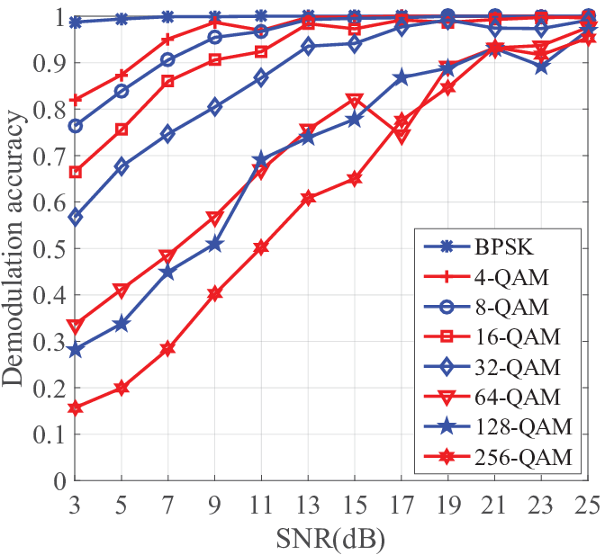
Fig. 9 presents the demodulation accuracies of BPSK and $M$ -QAM modulation schemes. In this experiment, the AdaBoost based demodulation algorithm was employed, where the number of sampling points is $N=40$ . The demodulation accuracy for all modulation schemes increases with SNR. Meanwhile, the accuracy achieved by the BPSK-modulation scheme is better than the other seven schemes for the same SNR. Furthermore, Fig. 9 also indicates that the demodulation accuracy reduces with an increase of the modulation order.

In Fig. 10, the same modulation schemes, demodulation algorithm, and sampling points are used as in Fig. 9, where the effective capacity of different modulation methods versus SNR are reported. The effective capacity by BPSK, $4$ -QAM, and $8$ -QAM almost remain unchanged with an increase in SNR. It is found that the modulation order has a considerable positive impact on the performance of the transmission capacity. The performance gap between the low order and the high order modulation is clearer when SNR $\leq 15$ dB. However, the demodulation accuracy of high order modulation is low, so there is a trade-off between the demodulation accuracy and the effective capacity.

VI Conclusion

In this paper, a flexible end-to-end wireless communications prototype platform was proposed for real physical environments. Then, the first open measured modulation data dataset with eight modulation schemes, i.e., BPSK, $4$ -QAM, $8$ -QAM, $16$ -QAM, $32$ -QAM, $64$ -QAM, $128$ -QAM, and $256$ -QAM, were established and accessed online. Furthermore, two DL-based demodulators, i.e., DBN-SVM based demodulator and AdaBoost based demodulator, were proposed. Based on the real dataset, the demodulation performance of the proposed demodulators were tested. Finally, experimental results indicated that the proposed demodulators outperform the DBN based, SVM based, and MLD based demodulators at various scenarios.

References

[1] J. G. Proakis, Digital communications, McGraw-Hill, New York, 2001.
[2] M. Shafi, A. F. Molisch, P. J. Smith, T. Haustein, P. Zhu, P. D. Silva, F. Tufvesson, A. Benjebbour, and G. Wunder, “5G : A Tutorial Overview of Standards, Trials, Challenges, Deployment, and Practice,” IEEE J. Select. Areas Commun., vol. 35, no. 6, pp. 1201–1221, Jun. 2017.
[3] Y. Lecun, Y. Bengio, and G. Hinton, “Deep learning.,” Nature, vol. 521, no. 7553, pp. 436, May 2015.
[4] C. Liu, Y. Cao, Y. Luo, G. Chen, V. Vokkarane, and Y. Ma, DeepFood: Deep Learning-Based Food Image Recognition for Computer-Aided Dietary Assessment, Springer, 2016.
[5] T. Zhou, S. Yang, L. Wang, J. Yao, and G. Gui, “Improved cross-label suppression dictionary learning for face recognition,” IEEE Access, vol. 6, pp. 48716–48725, Aug. 2018.
[6] D. Geronimo, J. Serrat, A. M. Lopez, and R. Baldrich, “Traffic sign recognition for computer vision project-based learning,” IEEE Trans. Educ., vol. 56, no. 3, pp. 364–371, Aug. 2013.
[7] T. Tan, Y. Qian, and K. Yu, “Cluster adaptive training for deep neural network based acoustic model,” IEEE Trans. Audio Speech Lang. Proces., vol. 24, no. 3, pp. 459–468, Mar. 2015.
[8] Y. Ling, C. Jin, G. Ding, Y. Tu, and J. Sun, “Spectrum prediction based on Taguchi method in deep learning with long short-term memory,” IEEE Access, vol. 6, pp. 45923–45933, Dec. 2018.
[9] H. Huang, W. Xia, J. Xiong, J. Yang, G. Zheng, and X. Zhu, “Unsupervised learning-based fast beamforming design for downlink MIMO,” IEEE Access, vol. 7, pp. 7599–7605, Jan. 2019.
[10] M. Liu, T. Song, and G. Gui, “Deep cognitive perspective: Resource allocation for NOMA based heterogeneous IoT with imperfect SIC,” IEEE Internet Things J., Oct. 2018.
[11] M. Liu, T. Song, J. Hu, J. Yang, and G. Gui, “Deep learning-inspired message passing algorithm for efficient resource allocation in cognitive radio networks,” IEEE Trans. Veh. Technol., vol. 68, no. 1, pp. 641–653, Jan. 2019.
[12] T. Oshea, J. Hoydis, T. Oshea, and J. Hoydis, “An introduction to deep learning for the physical layer,” IEEE Trans. Cogn. Commun. Netw., vol. 3, no. 4, pp. 563–575, Oct. 2017.
[13] S. Dörner, S. Cammerer, J. Hoydis, and S. t. Brink, “Deep learning based communication over the air,” IEEE J. Sel. Top. Sign. Proces., vol. 12, no. 1, pp. 132–143, Feb. 2018.
[14] T. Fath and H. Haas, “Performance comparison of MIMO techniques for optical wireless communications in indoor environments,” IEEE Trans. Commun., vol. 61, no. 2, pp. 733–742, Feb. 2013.
[15] T. Q. Wang, Y. A. Sekercioglu, and J. Armstrong, “Analysis of an optical wireless receiver using a hemispherical lens with application in MIMO visible light communications,” J. Lightw. Technol., vol. 31, no. 11, pp. 1744–1754, Jun. 2013.
[16] K. Ying, H. Qian, R. J. Baxley, and S. Yao, “Joint optimization of precoder and equalizer in MIMO VLC systems,” IEEE J. Select. Areas Commun., vol. 33, no. 9, pp. 1949–1958, Sept. 2015.
[17] H. Huang, J. Yang, H. Huang, Y. Song, and G. Gui, “Deep learning for super-resolution channel estimation and doa estimation based massive mimo system,” IEEE Trans. Veh. Technol., vol. 67, no. 9, pp. 8549–8560, Sep. 2018.
[18] J. Wang, J. Yang, J. Xiong, H. Sari, and G. Gui, “SHAFA: sparse hybrid adaptive filtering algorithm to estimate channels in various SNR environments,” IET Commun., vol. 12, no. 16, pp. 1963–1967, Sep. 2018.
[19] G. Gui, H. Huang, Y. Song, and H. Sari, “Deep learning for an effective nonorthogonal multiple access scheme,” IEEE Trans. Veh. Technol., vol. 67, no. 9, pp. 8440–8450, Sep. 2018.
[20] S. Schiessl, H. Al-Zubaidy, M. Skoglund, and J. Gross, “Delay performance of wireless communications with imperfect CSI and finite-length coding,” IEEE Trans. Commun., vol. 66, no. 12, pp. 6527–6541, Dec. 2018.
[21] T. Mitchell, B. Buchanan, G. Dejong, T. Dietterich, P. Rosenbloom, and A. Waibel, Machine Learning, China Machine Press, 2003.
[22] X. Lin, R. Liu, W. Hu, Y. Li, X. Zhou, and X. He, “A deep convolutional network demodulator for mixed signals with different modulation types,” in IEEE Int. Conf. on Dependable, Autonomic and Secure Computing, pp. 893–896, Nov. 2017.
[23] M. Fan and L. Wu, “Demodulator based on deep belief networks in communication system,” in IEEE Int. Conf. Communication, Control, Computing and Electronics Engineering, pp. 1–5, Jan. 2017.
[24] L. Fang and L. Wu, “Deep learning detection method for signal demodulation in short range multipath channel,” in IEEE Int. Conf. on Opto-Electronic Information Processing, pp. 16–20, Jul. 2017.
[25] A. S. Mohammad, N. Reddy, F. James, and C. Beard, “Demodulation of faded wireless signals using deep convolutional neural networks,” in IEEE Annu. Comput. and Commun. Workshop and Conf., pp. 969–975, Jan. 2018.
[26] Y. Freund and R. E. Schapire, “Experiments with a new boosting algorithm,” in Int. Conf. on Machine learning, pp. 148–156, Jul. 1996.
[27] M. Kulin, T. Kazaz, I. Moerman, and E. De Poorter, “End-to-end learning from spectrum data: A deep learning approach for wireless signal identification in spectrum monitoring applications,” IEEE Access, vol. 6, pp. 18484–18501, Mar. 2018.
[28] B. Karanov, M. Chagnon, F. Thouin, T. A. Eriksson, H. Bulow, D. Lavery, P. Bayvel, and L. Schmalen, “End-to-end deep learning of optical fiber communications,” J. Lightw. Technol., vol. 36, no. 20, pp. 4843–4855, Oct. 2018.
[29] Y. Lecun, U. Müller, J. Ben, E. Cosatto, and B. Flepp, “Off-road obstacle avoidance through end-to-end learning.,” in Proc. Adv. Neural Inf. Process. Syst., pp. 739–746, 2006.
[30] J. Sola and J. Sevilla, “Importance of input data normalization for the application of neural networks to complex industrial problems,” Nucl. Sci., vol. 44, no. 3, pp. 1464–1468, Jun. 1997.
[31] G. E. Hinton, “Training products of experts by minimizing contrastive divergence,” Neural Comput., vol. 14, no. 8, pp. 1771–1800, Feb. 2002.
[32] Z. Yang and X. Pang, “Research and implementation of text classification model based on combination of DAE and DBN,” in Int. Symp. Comput. Intell. Des., vol. 2, pp. 190–193, Dec. 2017.
[33] R. Sarikaya, G. E. Hinton, and A. Deoras, “Application of deep belief networks for natural language understanding,” IEEE Trans. Audio Speech Lang. Proces., vol. 22, no. 4, pp. 778–784, Aug. 2014.
[34] F. Zhang and Q. Zhou, “Ensemble detection model for profile injection attacks in collaborative recommender systems based on BP neural network,” IET Inf. Sec., vol. 9, no. 1, pp. 24–31, Dec. 2015.
[35] X. H. Wang, “Multi-class SVMs based on probability voting strategy and its application,” Comput. Eng., vol. 35, no. 2, pp. 180–183, Feb. 2009.
[36] J. C. Platt, N. Cristianini, and J. Shawe-Taylor, “Large margin DAGs for multiclass classification,” in Advances in neural inform. process. systems, pp. 547–553, Jan. 2000.
[37] A. Rhuma, S. M. Naqvi, and J. Chambers, “An improved directed acyclic graph support vector machine,” J. Measure. Sci. Instrum., vol. 2, no. 4, pp. 367–370, Dec. 2011.
[38] Y. Wang, L. Wang, J. Qiu, P. Shen, and D. U. Xin, “Research on pedestrian detection method based on multilayer RBM network and SVM,” Journal of the China Railway Society, Mar. 2018.
[39] R. A. Mcdonald, D. J. Hand, and I. A. Eckley, An Empirical Comparison of Three Boosting Algorithms on Real Data Sets with Artificial Class Noise, Springer, Berlin, Heidelberg, 2003.