A structure-preserving discontinuous Galerkin scheme for the Fisher-KPP equationThanks: The authors acknowledge partial support from the Austrian Science Fund (FWF), grant F65. The first author has been supported by the FWF Firnberg-Program, grant T998. The second and third authors acknowledge support from the FWF, grants P30000 and W1245. The forth author acknowledges support from the FWF, grant P29197-N32. The authors thank Clément Cancès for pointing out how to prove Proposition 15.

Francesca Bonizzoni Address: Faculty of Mathematics, University of Vienna, Oskar-Morgenstein-Platz 1, 1090 Wien, Austria Email address: francesca.bonizzoni@univie.ac.at , Marcel Braukhoff Address: Institute for Analysis and Scientific Computing, Vienna University of Technology, Wiedner Hauptstraße 8–10, 1040 Wien, Austria Email address: marcel.braukhoff@tuwien.ac.at , Ansgar Jüngel Address: Institute for Analysis and Scientific Computing, Vienna University of Technology, Wiedner Hauptstraße 8–10, 1040 Wien, Austria Email address: juengel@tuwien.ac.at and Ilaria Perugia Address: Faculty of Mathematics, University of Vienna, Oskar-Morgenstein-Platz 1, 1090 Wien, Austria Email address: ilaria.perugia@univie.ac.at

Date: August 11, 2026

Abstract.

An implicit Euler discontinuous Galerkin scheme for the Fisher-Kolmogorov-Petrovsky-Piscounov (Fisher-KPP) equation for population densities with no-flux boundary conditions is suggested and analyzed. Using an exponential variable transformation, the numerical scheme automatically preserves the positivity of the discrete solution. A discrete entropy inequality is derived, and the exponential time decay of the discrete density to the stable steady state in the $L^{1}$ norm is proved if the initial entropy is smaller than the measure of the domain. The discrete solution is proved to converge in the $L^{2}$ norm to the unique strong solution to the time-discrete Fisher-KPP equation as the mesh size tends to zero. Numerical experiments in one space dimension illustrate the theoretical results.

Key words and phrases:

Positivity preservation, entropy variables, discontinuous Galerkin method, discrete entropy decay, convergence of the scheme.

2000 Mathematics Subject Classification

65M60, 65M12, 35K20, 35K57.

1. Introduction

The preservation of the structure of nonlinear diffusion equations on the discrete level is of paramount importance in applications. While there has been an enormous progress on structure-preserving schemes for ordinary differential equations (see, e.g., [16]), the development of structure-preserving numerical techniques for nonlinear diffusion equations is still an ongoing quest, in particular for higher-order methods. In this paper, we analyze a toy problem, the Fisher-Kolmogorov-Petrovsky-Piscounov (Fisher-KPP) equation with no-flux boundary conditions, to devise an implicit Euler discontinuous Galerkin scheme which preserves the positivity of the solution, the entropy structure, and the exponential equilibration on the discrete level. In a future work, we aim to extend the scheme to diffusion systems.

The Fisher-KPP equation [12] is the reaction-diffusion equation

(1)			$\displaystyle\partial_{t}u=D\Delta u+u(1-u)\quad\mbox{in }\Omega,\ t>0,$
(2)			$\displaystyle\nabla u\cdot n=0\quad\mbox{on }\partial\Omega,\quad u(0)=u_{0}\quad\mbox{in }\Omega,$

where $D>0$ is the diffusion coefficient, $\Omega\subset{\mathbb{R}}^{d}$ a bounded domain, and $n$ the exterior unit normal vector on the boundary $\partial\Omega$ . The variable $u(x,t)$ models a population density or chemical concentration, influenced by diffusion and logistic growth. The Fisher-KPP equation admits traveling-wave solutions $u(x,t)=\phi(x-ct)$ , which switch between the unstable steady state $u^{*}=0$ and the stable steady state $u^{*}=1$ . By the maxiumum principle, the density stays nonnegative if it does so initially, and it satisfies the entropy inequality

(3)

\frac{d}{dt}\int_{\Omega}u(\log u-1)dx+D\int_{\Omega}\frac{|\nabla u|^{2}}{u}dx=-\int_{\Omega}u(u-1)\log udx\leq 0.

If there are no reaction terms, we have conservation of the total mass, and the logarithmic Sobolev inequality implies the exponential decay of the (mathematical) entropy $S(t)=\int_{\Omega}(u(t)(\log u(t)-1)+1)dx$ (see, e.g., [20, Chapter 2]). When reaction terms are present, the situation is more delicate, since there are two steady states, $u^{*}=0$ and $u^{*}=1$ . If the initial entropy $S(0)$ is smaller than the measure of $\Omega$ , then $u(t)$ converges exponentially fast to $u^{*}=1$ in the $L^{1}(\Omega)$ norm. Our objective is to preserve the aforementioned properties on the discrete level.

It is well known that the preservation of the positivity or nonnegativity of discrete solutions for (1) may fail in standard (finite-element) schemes, in particular when the solution vanishes in some region; see Section 5 for an example. Our key idea to preserve the positivity is to employ the exponential transformation $u=e^{\lambda}$ . Such a transformation or a variant is used, for instance, in the Il’in scheme [19] and in the existence analysis of drift-diffusion equations [13]. Moreover, it allows for the preservation of $L^{\infty}(\Omega)$ bounds in volume-filling cross-diffusion systems [8, 20]. The implicit Euler scheme for (1)-(2) in the exponential variable then reads as

(4)		$\displaystyle\frac{1}{\triangle t}\big(e^{\lambda^{k}}-e^{\lambda^{k-1}}\big)$	$\displaystyle=\operatorname{div}(e^{\lambda^{k}}\nabla e^{\lambda^{k}})+e^{\lambda^{k}}(1-e^{\lambda^{k}})\quad\mbox{in }\Omega,$
(5)		$\displaystyle\nabla\lambda^{k}\cdot n$	$\displaystyle=0\quad\mbox{on }\partial\Omega,$

where here and in the following, we set $D=1$ for simplicity and we choose $0<\triangle t<1$ . At first glance, one may think that this formulation unnecessarily complicates the problem, but we will show that it enjoys some useful properties.

We propose a discontinuous Galerkin (DG) discretization for problem (4)-(5) with variable $\lambda_{h}^{k}$ , where $h>0$ is the maximal diameter of the mesh elements. The nonlinear diffusion term is discretized by an interior penalty DG method. By construction, the discrete densities $\exp(\lambda_{h}^{k})$ are positive, and the scheme also preserves the entropy structure and large-time asymptotics. Our main results can be sketched as follows:

•

Existence of a solution $\lambda_{h}^{k}$ to the implicit Euler DG scheme (8), given a function $\lambda_{h}^{k-1}$ (Proposition 6). This result is based on the Leray-Schauder fixed-point theorem and a coercivity estimate.
•

Discrete entropy inequality (Lemma 7). The inequality follows from scheme (8) using the test function $\lambda_{h}^{k}$ and the convexity of $u\mapsto u(\log u-1)+1$ .
•

Exponential decay of the discrete entropy

$S_{h}^{k}:=\int_{\Omega}\big(e^{\lambda_{h}^{k}}(e^{\lambda_{h}^{k}}-1)+1\big)dx\leq S_{h}^{0}e^{-\kappa k\triangle t}$

(Proposition 9) and of the $L^{1}$ norm of $e^{\lambda_{h}^{k}}-1$ (Theorem 11). The result holds if $S_{h}^{0}<|\Omega|$ . This condition implies a positive lower bound for the total mass $\int_{\Omega}e^{\lambda_{h}^{k}}dx$ , which is needed to guarantee that the discrete solution converges to the stable steady state $u^{*}=1$ and not to the steady state $u^{*}=0$ . The case $S_{h}^{0}\geq|\Omega|$ is discussed in Remark 12.
•

Convergence of the scheme (Theorem 14): There exists a unique strong solution $u^{k}\in H^{2}_{n}(\Omega)$ to the implicit Euler discretization associated to (1)-(2) such that

$e^{\lambda_{h}^{k}}\to u^{k}\quad\mbox{strongly in }L^{2}(\Omega)\mbox{ as }h\to 0.$

The result is based on a compactness property, which is a consequence of the gradient estimate from the entropy inequality and a coercivity estimate. This yields a very weak semi-discrete solution, which turns out to be a strong solution thanks to a duality argument.

Let us put our results into context and review the state of the art of stucture preservation in DG methods. The DG scheme was introduced in the early 1970s for first-order hyperbolic problems in [22, 31]. The development of discontinuous finite-element schemes for second-order elliptic problems can be traced back to [27] with similar approaches in, for instance, [2, 5, 29, 34]; see also [3].

The design of structure-preserving DG methods is a rather recent topic. Positivity-preserving DG schemes for parabolic equations were developed in, e.g., [9, 15, 23, 33, 36]. The positivity preservation is ensured by using a special slope limiter (as in [9, 15]), together with a strong stability preserving Runge-Kutta time discretization (as in [33, 36]), while in [23], the positivity of the discrete solution is enforced through a reconstruction algorithm, based on positive cell averages. As far as we know, the use of an exponential transformation to ensure the positivity of the discrete solutions within a DG scheme is new. Positivity-preserving schemes for the Fisher-KPP equation were already studied in the literature, but only for finite-difference approximations [17, 24], without a convergence analysis, and for continuous finite-element discretizations [35].

Other important properties are entropy stability (the entropy is bounded for all times) and entropy monotonicity (the entropy is nonincreasing). Entropy-stable DG schemes for the compressible Euler and Navier-Stokes equation were studied in [14, 28], while a discrete version of the entropy inequality (and hence entropy monotonicity) was proved in [33] for Fokker-Planck-type equations and aggregation models. We are not aware of results in the literature regarding the preservation of the entropy structure of the Fisher-KPP equation on the discrete level.

The paper is organized as follows. We state our notation and some auxiliary results related to the DG method in Section 2. The DG scheme is introduced and studied in Section 3: The existence of a solution to the DG scheme, the discrete entropy inequality, and the exponential decay of the entropy are proved. The convergence of the numerical scheme is proved in Section 4. Finally, Section 5 is devoted to some numerical experiments in one space dimension.

2. Notation and auxiliary results

We start with some notation. Let $\mathcal{T}_{h}=\{K_{i}:i=1,\ldots,N_{h}\}$ be a family of simplicial partitions of the bounded domain $\Omega\subset{\mathbb{R}}^{d}$ for $d=1,2,3$ . The mesh parameter $h$ is defined by $h=\max_{K\in\mathcal{T}_{h}}h_{K}$ , where $h_{K}=\operatorname{diam}(K)$ . The elements may be tetrahedra in three space dimensions, triangles in two dimensions, and intervals in one dimension. In two and three dimensions, we suppose that $\mathcal{T}_{h}$ is shape regular (see, e.g., [30, Section 2.1]) and, for simplicity, without hanging nodes. Our analysis actually extends also to $k$ -irregular meshes [18]. We denote by $\mathcal{E}_{h}$ the set of interior faces or edges of the elements in $\mathcal{T}_{h}$ .

On the partition $\mathcal{T}_{h}$ , we define the broken Sobolev space

H^{s}(\Omega,\mathcal{T}_{h})=\big\{\xi\in L^{2}(\Omega):\xi|_{K}\in H^{s}(K)\mbox{ for all }K\in\mathcal{T}_{h}\big\},\quad s>0.

The traces of functions in $H^{1}(\Omega,\mathcal{T}_{h})$ belong to the space $T(\Gamma_{h})=\prod_{K\in\mathcal{T}_{h}}L^{2}(\partial K)$ , where $\Gamma_{h}$ is the union of all boundaries $\partial K$ for all $K\in\mathcal{T}_{h}$ . The functions in $T(\Gamma_{h})$ are single-valued on $\partial\Omega$ and double-valued on $\Gamma_{h}\setminus\partial\Omega$ .

Let $q$ be a piecewise smooth function and $q$ be a piecewise smooth vector field on $\mathcal{T}_{h}$ . We write $K_{-}$ and $K_{+}$ for the two elements sharing the face $f$ , i.e. $f=\partial K_{-}\cap\partial K_{+}$ , and $n_{\pm}$ for the unit normal vector pointing to the exterior of $K_{\pm}$ . Furthermore, we set $q_{\pm}=q|_{K_{\pm}}$ and $\phi_{\pm}=\phi|_{K_{\pm}}$ . Then we define

	averages:	$\displaystyle\{q\}=\frac{1}{2}(q_{-}+q_{+}),\quad\{\phi\}=\frac{1}{2}(\phi_{-}+\phi_{+}),$
	jumps:	$\displaystyle\ldbrack q\rdbrack=q_{-}n_{-}+q_{+}n_{+},\quad\ldbrack\phi\rdbrack=\phi_{-}\cdot n_{-}+\phi_{+}\cdot n_{+}.$

Note that the jump of a scalar function is a vector which is normal to $f$ , and the jump of a vector-valued function is a scalar.

The mesh size function ${\tt h}\in L^{\infty}(\Gamma_{h})$ is defined by

{\tt h}(x)=\min\{h_{K_{-}},h_{K_{+}}\}\quad\mbox{for }x\in\partial K_{-}\cap\partial K_{+}.

Furthermore, we introduce the finite-element space of degree $p\in{\mathbb{N}}$ associated to the partition $\mathcal{T}_{h}$ :

V_{h}=\big\{v\in L^{2}(\Omega):v|_{K}\in P_{p}(K)\mbox{ for all }K\in\mathcal{T}_{h}\big\},

where $P_{p}(K)$ is the set of polynomials on $K$ with degree at most $p$ , and the space of test functions

H_{n}^{2}(\Omega)=\{\phi\in H^{2}(\Omega):\nabla\phi\cdot n=0\mbox{ on }\partial\Omega\}.

Next, we recall some auxiliary results.

Lemma 1 (Inverse trace inequality; Lemma 2.1 in [32]).

Let $K\in{\mathbb{R}}^{d}$ ( $d=2,3$ ) be an element with diameter $h_{K}$ , let $f$ be an edge or face of $K$ , and let $n_{f}$ be a unit normal vector normal to $f$ . Then for all polynomials $\xi\in P_{p}(K)$ of degree $p$ , there exists a constant $C_{\rm inv}>0$ , independent of $h_{K}$ and $p$ , such that

(6)		$\displaystyle\\|\xi\\|_{L^{2}(\partial K)}$	$\displaystyle\leq C_{\rm inv}\frac{p}{\sqrt{h_{K}}}\\|\xi\\|_{L^{2}(K)},$
	$\displaystyle\\|\nabla\xi\cdot n_{f}\\|_{L^{2}(\partial K)}$	$\displaystyle\leq C_{\rm inv}\frac{p}{\sqrt{h_{K}}}\\|\nabla\xi\\|_{L^{2}(K)}.$

Lemma 2 (Multiplicative trace inequality; Lemma A.2 in [30]).

Let $K$ be a shape-regular element. Then there exists a constant $C>0$ such that for all $\xi\in H^{1}(K)$ ,

\|\xi\|_{L^{2}(\partial K)}^{2}\leq C\|\xi\|_{L^{2}(K)}\bigg(\frac{1}{h_{K}}\|\xi\|_{L^{2}(K)}+\|\nabla\xi\|_{L^{2}(K)}\bigg).

Lemma 3 (Discrete Poincaré-Wirtinger inequality; Theorem 4.1 in [7]).

There exists a constant $C_{\rm PW}>0$ such that for all $\xi\in H^{1}(\Omega,\mathcal{T}_{h})$ ,

\bigg\|\xi-\frac{1}{|\Omega|}\int_{\Omega}\xi dx\bigg\|_{L^{2}(\Omega)}\leq C_{\rm PW}\bigg(\sum_{K\in\mathcal{T}_{h}}\|\nabla\xi\|_{L^{2}(K)}^{2}+\sum_{f\in\mathcal{E}_{h}}\int_{f}\frac{p^{2}}{{\tt h}}|\ldbrack\xi\rdbrack|^{2}dx\bigg)^{1/2}.

We also need a compactness result for functions $\xi\in H^{1}(\Omega,\mathcal{T}_{h})$ . For this, we define the DG norm

(7)

\|\xi\|_{\rm DG}=\bigg(\|\xi\|_{L^{2}(\Omega)}^{2}+\sum_{K\in\mathcal{T}_{h}}\|\nabla\xi\|_{L^{2}(K)}^{2}+\sum_{f\in\mathcal{E}_{h}}\int_{f}\frac{p^{2}}{{\tt h}}|\ldbrack\xi\rdbrack|^{2}dx\bigg)^{1/2}.

Lemma 4 (DG compact embedding; Lemma 8 in [7]).

Let $(\xi_{h})\subset H^{1}(\Omega,\mathcal{T}_{h})$ be a sequence such that $\|\xi_{h}\|_{\rm DG}\leq C$ for all $h\in(0,1)$ and some $C>0$ . Then there exists a subsequence $(h_{i})$ with $h_{i}\to 0$ as $i\to\infty$ and a function $\xi\in H^{1}(\Omega)$ such that

\xi_{h_{i}}\to\xi\quad\mbox{strongly in }L^{q}(\Omega)\mbox{ as }h_{i}\to 0,

where $1\leq q<q^{*}$ and $q^{*}=4$ for $d=3$ , $q^{*}=\infty$ for $d=1,2$ .

3. Analysis of the DG scheme: existence and structure preservation

The DG discretization of the weak formulation of (4)-(5) reads as follows. Let $\varepsilon\geq 0$ and $\lambda_{h}^{0}\in V_{h}$ . Given $\lambda_{h}^{k-1}\in V_{h}$ , we wish to find $\lambda_{h}^{k}\in V_{h}$ such that for all $\phi_{h}\in V_{h}$ ,

(8)

\int_{\Omega}\big(e^{\lambda_{h}^{k}}-e^{\lambda_{h}^{k-1}}\big)\phi_{h}dx+\triangle tB(\lambda_{h}^{k};\lambda_{h}^{k},\phi_{h})+\varepsilon\int_{\Omega}\lambda_{h}^{k}\phi_{h}dx=\triangle t\int_{\Omega}e^{\lambda_{h}^{k}}(1-e^{\lambda_{h}^{k}})\phi_{h}dx.

The form $B:H^{1}(\Omega,\mathcal{T}_{h})^{3}\to{\mathbb{R}}$ represents the interior penalty DG discretization of the nonlinear diffusion term. It is linear in the second and third argument and is defined by

	$\displaystyle B(u;v,w)$	$\displaystyle=\sum_{K\in\mathcal{T}_{h}}e^{u}\nabla v\cdot\nabla wdx-\sum_{f\in\mathcal{E}_{h}}\int_{f}\big(\{e^{u}\nabla v\}\cdot\ldbrack w\rdbrack+\{e^{u}\nabla w\}\cdot\ldbrack v\rdbrack\big)ds$
(9)			$\displaystyle\phantom{xx}{}+\sum_{f\in\mathcal{E}_{h}}\int_{f}\frac{p^{2}}{{\tt h}}\alpha(u)\ldbrack v\rdbrack\cdot\ldbrack w\rdbrack ds,$

where $\alpha(u)$ is a stabilization function, given by

(10)

\alpha(u)=\frac{3}{2}C_{\rm inv}^{2}\big(\max\{(e^{u})_{-},(e^{u})_{+}\}\big)^{2}\max\big\{\exp(\|u\|_{L^{\infty}(K_{-})}),\exp(\|u\|_{L^{\infty}(K_{+})})\big\}.

We recall that the constant $C_{\rm inv}$ is defined in Lemma 1. The third term on the left-hand side of (8) is a regularization term (only) needed for the existence analysis to derive a uniform (but $\varepsilon$ -depending) bound for the fixed-point argument. For linear elements $p=1$ , we may allow for $\varepsilon=0$ ; see Appendix A.

3.1. Existence of a discrete solution

We show that problem (8) possesses a solution. First, we prove a coercivity property for the form $B$ .

Lemma 5 (Coercivity of $B$ ).

The form $B$ , defined in (9), satisfies for all $v\in H^{1}(\Omega,\mathcal{T}_{h})$ ,

B(v;v,v)\geq 2\sum_{K\in\mathcal{T}_{h}}\int_{K}|\nabla e^{v/2}|^{2}dx+2C_{\rm inv}^{2}\sum_{f\in\mathcal{E}_{h}}\int_{f}\frac{p^{2}}{{\tt h}}|\ldbrack e^{v/2}\rdbrack|^{2}ds.

Proof.

Definition (9) gives for $v\in H^{1}(\Omega,\mathcal{T}_{h})$ :

(11)

B(v;v,v)=\sum_{K\in\mathcal{T}_{h}}\int_{K}e^{v}|\nabla v|^{2}dx-2\sum_{f\in\mathcal{E}_{h}}\int_{f}\{e^{v}\nabla v\}\cdot\ldbrack v\rdbrack ds+\sum_{f\in\mathcal{E}_{h}}\int_{f}\frac{p^{2}}{{\tt h}}\alpha(v)|\ldbrack v\rdbrack|^{2}ds

We estimate the second integral by using Young’s inequality:

2\sum_{f\in\mathcal{E}_{h}}\int_{f}\{e^{v}\nabla v\}\cdot\ldbrack v\rdbrack ds\leq\sum_{f\in\mathcal{E}_{h}}\bigg(\int_{f}\beta_{f}^{2}\{e^{v}\nabla v\}^{2}ds+\int_{f}\frac{1}{\beta_{f}^{2}}|\ldbrack v\rdbrack|^{2}ds\bigg),

where $\beta_{f}>0$ is a parameter which will be defined below. The first integral on the right-hand side is estimated according to

	$\displaystyle\sum_{f\in\mathcal{E}_{h}}\int_{f}\beta_{f}^{2}\{e^{v}\nabla v\}^{2}ds$	$\displaystyle=\frac{1}{4}\sum_{f\in\mathcal{E}_{h}}\int_{f}\beta_{f}^{2}\big\|(e^{v}\nabla v)_{-}+(e^{v}\nabla v)_{+}\big\|^{2}ds$
		$\displaystyle\leq\frac{1}{2}\sum_{f\in\mathcal{E}_{h}}\int_{f}\beta_{f}^{2}\big(\|(e^{v}\nabla v)_{-}\|^{2}+\|(e^{v}\nabla v)_{+}\|^{2}\big)ds$
		$\displaystyle=\frac{1}{2}\sum_{f\in\mathcal{E}_{h}}\int_{f}\beta_{f}^{2}\big(\max\{(e^{v})_{-},(e^{v})_{+}\}\big)^{2}\big(\|(\nabla v)_{-}\|^{2}+\|(\nabla v)_{+}\|^{2}\big)ds.$

To proceed, we set

\beta_{f}:=\frac{\min\{\gamma_{K_{-}},\gamma_{K_{+}}\}}{\max\{(e^{v})_{-},(e^{v})_{+}\}},\quad\mbox{where }\gamma_{K}^{2}:=\frac{h_{K}}{C_{\rm inv}^{2}p^{2}}\exp(-\|v\|_{L^{\infty}(K)}).

Taking into account the inverse trace inequality (6), we infer that

	$\displaystyle\sum_{f\in\mathcal{E}_{h}}\int_{f}\beta_{f}^{2}\{e^{v}\nabla v\}^{2}ds$	$\displaystyle\leq\frac{1}{2}\sum_{K\in\mathcal{T}_{h}}\int_{\partial K}\gamma_{K}^{2}\|\nabla v\|^{2}ds\leq\frac{1}{2}C_{\rm inv}^{2}\sum_{K\in\mathcal{T}_{h}}\gamma_{K}^{2}\frac{p^{2}}{h_{K}}\int_{K}\|\nabla v\|^{2}dx$
		$\displaystyle\leq\frac{1}{2}C_{\rm inv}^{2}p^{2}\sum_{K\in\mathcal{T}_{h}}\frac{\gamma_{K}^{2}}{h_{K}}\exp(\\|v\\|_{L^{\infty}(K)})\int_{K}e^{v}\|\nabla v\|^{2}dx$
		$\displaystyle=\frac{1}{2}\sum_{K\in\mathcal{T}_{h}}\int_{K}e^{v}\|\nabla v\|^{2}dx.$

Consequently, we obtain

2\sum_{f\in\mathcal{E}_{h}}\int_{f}\{e^{v}\nabla v\}\cdot\ldbrack v\rdbrack ds\leq\sum_{f\in\mathcal{E}_{h}}\int_{f}\frac{1}{\beta_{f}^{2}}|\ldbrack v\rdbrack|^{2}ds+\frac{1}{2}\sum_{K\in\mathcal{T}_{h}}\int_{K}e^{v}|\nabla v|^{2}dx.

Inserting this estimate into (11), it follows that

B(v;v,v)\geq\frac{1}{2}\sum_{K\in\mathcal{T}_{h}}e^{v}|\nabla v|^{2}dx+\sum_{f\in\mathcal{E}_{h}}\int_{f}\bigg(\frac{p^{2}}{{\tt h}}\alpha(v)-\frac{1}{\beta_{f}^{2}}\bigg)|\ldbrack v\rdbrack|^{2}ds.

With the definitions of $\alpha(v)$ (see (10)) and $\beta_{f}$ as well as the property ${\tt h}\leq h_{K_{\pm}}$ , the difference in the bracket can be computed as

	$\displaystyle\frac{p^{2}}{{\tt h}}\alpha(v)-\frac{1}{\beta_{f}^{2}}$	$\displaystyle\geq\frac{3}{2}\frac{p^{2}}{{\tt h}}C_{\rm inv}^{2}\big(\max\{(e^{v})_{-},(e^{v})_{+}\}\big)^{2}\max\big\{\exp(\\|v\\|_{L^{\infty}(K_{-})}),\exp(\\|v\\|_{L^{\infty}(K_{+})})\big\}$
		$\displaystyle\phantom{xx}{}-\frac{C_{\rm inv}^{2}p^{2}(\max\{(e^{v})_{-},(e^{v})_{+}\})^{2}}{\min\{h_{K_{-}}\exp(-\\|v\\|_{L^{\infty}(K_{-})}),h_{K_{+}}\exp(-\\|v\\|_{L^{\infty}(K_{+})})\}}$
		$\displaystyle\geq\frac{p^{2}}{2{\tt h}}C_{\rm inv}^{2}(\max\{(e^{v})_{-},(e^{v})_{+}\})^{2}\max\big\{\exp(\\|v\\|_{L^{\infty}(K_{-})}),\exp(\\|v\\|_{L^{\infty}(K_{+})})\big\}$
		$\displaystyle=\frac{1}{3}\frac{p^{2}}{{\tt h}}\alpha(v).$

This shows that

(12)

B(v;v,v)\geq 2\sum_{K\in\mathcal{T}_{h}}\int_{K}|\nabla e^{v/2}|^{2}dx+\frac{1}{3}\sum_{f\in\mathcal{E}_{h}}\int_{f}\frac{p^{2}}{{\tt h}}\alpha(v)|\ldbrack v\rdbrack|^{2}ds.

By the definition of the jumps and the mean-value theorem for $x\in f$ ,

|\ldbrack e^{v/2}\rdbrack|^{2}=\big|e^{v_{-}/2}-e^{v_{+}/2}\big|^{2}\leq\frac{1}{4}\max\{e^{v_{-}},e^{v_{+}}\}|\ldbrack v\rdbrack|^{2}.

We use definition (10) and insert the previous estimate into (12):

	$\displaystyle B(v;v,v)$	$\displaystyle\geq 2\sum_{K\in\mathcal{T}_{h}}\int_{K}\|\nabla e^{v/2}\|^{2}dx+2C_{\rm inv}^{2}\sum_{f\in\mathcal{E}_{h}}\int_{f}\frac{p^{2}}{{\tt h}}\max\{(e^{v})_{-},(e^{v})_{+}\}$
		$\displaystyle\phantom{xx}{}\times\max\big\{\exp(\\|v\\|_{L^{\infty}(K_{-})}),\exp(\\|v\\|_{L^{\infty}(K_{+})})\big\}\|\ldbrack e^{v/2}\rdbrack\|^{2}ds.$

Since $(e^{v})_{\pm}\geq\exp(-\|v\|_{L^{\infty}(K_{\pm})})$ , we have

\max\{(e^{v})_{-},(e^{v})_{+}\}\max\big\{\exp(\|v\|_{L^{\infty}(K_{-})}),\exp(\|v\|_{L^{\infty}(K_{+})})\big\}\geq 1.

This finishes the proof. ∎

Proposition 6 (Existence).

Let $\varepsilon>0$ . Given $\lambda_{h}^{k-1}\in V_{h}$ , the DG scheme (8) admits a solution $\lambda_{h}^{k}\in V_{h}$ .

Proof.

The idea is to apply the Leray-Schauder fixed-point theorem. We define the fixed-point operator $\Phi:V_{h}\times[0,1]\to V_{h}$ by $\Phi(w,\sigma)=w$ , where $v\in V_{h}$ is the unique solution to the linear problem

(13)

\varepsilon\int_{\Omega}v\phi dx=\sigma\int_{\Omega}\big(e^{\lambda_{h}^{k-1}}-e^{w}+\triangle te^{w}(1-e^{w})\big)\phi dx-\sigma\triangle tB(w;w,\phi)

for $\phi\in V_{h}$ . The left-hand side defines the bilinear form $a(w,\phi)$ , which is coercive, $a(w,w)=\varepsilon\|w\|_{L^{2}(\Omega)}^{2}$ . The right-hand side defines a linear form which is continuous on $L^{2}(\Omega)$ (using the fact that in finite dimensions, all norms are equivalent). Thus, $\Phi$ is well defined by the Lax-Milgram lemma. As the right-hand side of (13) is continuous with respect to $w$ , standard arguments show that $\Phi$ is continuous. Furthermore, $\Phi(w,0)=0$ . It remains to prove that there exists a uniform bound for all fixed points of $\Phi$ . To this end, let $v\in V_{h}$ and $\sigma\in[0,1]$ such that $\Phi(v,\sigma)=v$ .

Let $s(v)=v(\log v-1)+1\geq 0$ . The convexity of $s$ implies that

(14)

(e^{\lambda_{h}^{k-1}}-e^{v})v=(e^{\lambda_{h}^{k-1}}-e^{v})s^{\prime}(e^{v})\leq s(e^{\lambda_{h}^{k-1}})-s(e^{v}).

Then, using the test function $\phi=v$ in (13) gives, because of the properties $B(v;v,v)\geq 0$ (Lemma 5) and $e^{v}(1-e^{v})v\leq 0$ ,

	$\displaystyle\varepsilon\\|v\\|_{L^{2}(\Omega)}^{2}$	$\displaystyle=\sigma\int_{\Omega}(e^{\lambda_{h}^{k-1}}-e^{v})vdx+\sigma\triangle t\int_{\Omega}e^{v}(1-e^{v})vdx-\sigma\triangle tB(v;v,v)$
(15)			$\displaystyle\leq\sigma\int_{\Omega}\big(s(e^{\lambda_{h}^{k-1}})-s(e^{v})\big)dx\leq\sigma\int_{\Omega}s(e^{\lambda_{h}^{k-1}})dx.$

This is the desired uniform bound. We infer the existence of a solution to (8) by the Leray-Schauder fixed-point theorem. ∎

3.2. Discrete entropy inequality and exponential decay

Let $\lambda_{h}^{k}\in V_{h}$ be a solution to (8). We show that the entropy

S_{h}^{k}:=\int_{\Omega}s(e^{\lambda_{h}^{k}})dx,\quad\mbox{where }s(u)=u(\log u-1)+1,

is nonincreasing with respect to $k\in{\mathbb{N}}$ .

Lemma 7 (Discrete entropy inequality).

Let $\varepsilon\geq 0$ and let $\lambda_{h}^{k}\in V_{h}$ be a solution to (8). Then

(16)

S_{h}^{k}+C_{0}\triangle t\int_{\Omega}\bigg|e^{\lambda_{h}^{k}/2}-\frac{1}{|\Omega|}\int_{\Omega}e^{\lambda_{h}^{k}/2}dy\bigg|^{2}dx+\triangle t\int_{\Omega}e^{\lambda_{h}^{k}}(e^{\lambda_{h}^{k}}-1)\lambda_{h}^{k}dx\leq S_{h}^{k-1},

where the constant $C_{0}>0$ only depends on $C_{\rm inv}$ and $C_{\rm PW}$ from Lemmas 1 and 3.

Proof.

We take $\phi_{h}=\lambda_{h}^{k}$ as a test function in (8) and use inequality (14) to find that

	$\displaystyle S_{h}^{k}-S_{h}^{k-1}$	$\displaystyle=\int_{\Omega}\big(s(e^{\lambda_{h}^{k}})-s(e^{\lambda_{h}^{k-1}})\big)dx$
		$\displaystyle=-\triangle tB(\lambda_{h}^{k};\lambda_{h}^{k},\lambda_{h}^{k})-\varepsilon\int_{\Omega}(\lambda_{h}^{k})^{2}dx-\triangle t\int_{\Omega}e^{\lambda_{h}^{k}}(e^{\lambda_{h}^{k}}-1)dx$
(17)			$\displaystyle\leq-\triangle tB(\lambda_{h}^{k};\lambda_{h}^{k},\lambda_{h}^{k})-\triangle t\int_{\Omega}e^{\lambda_{h}^{k}}(e^{\lambda_{h}^{k}}-1)\lambda_{h}^{k}\lambda_{h}^{k}dx.$

It remains to estimate the first term on the right-hand side. For this, we use the coercivity estimate of Lemma 5 and the discrete Poincaré-Wirtinger inequality from Lemma 3:

	$\displaystyle B(\lambda_{h}^{k};\lambda_{h}^{k},\lambda_{h}^{k})$	$\displaystyle\geq 2\min\{1,C_{\rm inv}^{2}\}\bigg(\sum_{K\in\mathcal{T}_{h}}\int_{K}\|\nabla e^{\lambda_{h}^{k}/2}\|^{2}dx+\sum_{f\in\mathcal{E}_{h}}\int_{f}\frac{p^{2}}{{\tt h}}\|\ldbrack e^{\lambda_{h}^{k}/2}\rdbrack\|^{2}ds\bigg)$
		$\displaystyle\geq 2\min\{1,C_{\rm inv}^{2}\}C_{\rm PW}^{-2}\int_{\Omega}\bigg\|e^{\lambda_{h}^{k}/2}-\frac{1}{\|\Omega\|}\int_{\Omega}e^{\lambda_{h}^{k}/2}dx\bigg\|^{2}dx.$

Setting $C_{0}=2\min\{1,C_{\rm inv}^{2}\}C_{\rm PW}^{-2}$ finishes the proof. ∎

We wish to bound the total mass $\int_{\Omega}\exp(\lambda_{h}^{k})dx$ from below and above. Since $s(u)=u(\log u-1)+1$ is invertible only on $[0,1]$ and on $[1,\infty)$ but not globally on $[0,\infty)$ , we introduce the following functions:

		$\displaystyle\sigma_{-}:[0,\infty)\to[0,1],\quad\sigma_{-}(v)=(s\|_{[0,1]})^{-1}(v)\mbox{ for }v\in[0,1],\ \sigma_{-}(v)=0\mbox{ for }v\in[1,\infty),$
		$\displaystyle\sigma_{+}:[0,\infty)\to[1,\infty),\quad\sigma_{+}(v)=(s\|_{[1,\infty)})^{-1}(v)\mbox{ for }v\in[0,\infty).$

In particular, $\sigma_{-}\circ s=\mbox{id}$ on $[0,1]$ and $\sigma_{+}\circ s=\mbox{id}$ on $[1,\infty)$ .

Lemma 8 (Bounds for the total mass).

Let $\varepsilon\geq 0$ and let $\lambda_{h}^{k}$ be a solution to (8). Then

\sigma_{-}\bigg(\frac{S_{h}^{0}}{|\Omega|}\bigg)\leq\frac{1}{|\Omega|}\int_{\Omega}e^{\lambda_{h}^{k}}dx\leq\sigma_{+}\bigg(\frac{S_{h}^{0}}{|\Omega|}\bigg).

Observe that if $S_{h}^{0}<|\Omega|$ , the lower bound $\sigma_{-}(S_{h}^{0}/|\Omega|)$ is positive. Thus, the total mass can never vanish, which excludes the case of solutions converging for $k\to\infty$ to the zero solution. The reason for the difference between $S_{h}^{0}<|\Omega|$ and $S_{h}^{0}\geq|\Omega|$ lies in the fact that (4)-(5) admits two steady states, $\lambda^{k}_{h}=0$ (corresponding to $u^{k}=e^{\lambda^{k}_{h}}=1$ ) and $\lambda^{k}_{h}=-\infty$ (corresponding to $u^{k}=0$ ). The assumption $S_{h}^{0}<|\Omega|$ will be crucial to prove the decay estimate for the entropy; see Proposition 9. We discuss the case $S_{h}^{0}\geq|\Omega|$ in Remark 12.

Proof of Lemma 8.

First, we show the lower bound. If $S_{h}^{0}\geq|\Omega|$ , we have $\sigma_{-}(S_{h}^{0}/|\Omega|)=0$ , and there is nothing to prove. Thus, let $S_{h}^{0}<|\Omega|$ . Set $\beta_{k}=\min\{1,\exp(\lambda_{h}^{k})\}\leq 1$ . As $s$ is convex, we infer from Jensen’s inequality and $s(\beta_{k})=0$ for $\lambda_{h}^{k}>0$ that

s\bigg(\frac{1}{|\Omega|}\int_{\Omega}\beta_{k}dx\bigg)\leq\frac{1}{|\Omega|}\int_{\Omega}s(\beta_{k})dx=\frac{1}{|\Omega|}\int_{\{\lambda_{h}^{k}\leq 0\}}s(e^{\lambda_{h}^{k}})dx\leq\frac{S_{h}^{k}}{|\Omega|}\leq\frac{S_{h}^{0}}{|\Omega|},

where in the last step we have used the monotonicity of $k\mapsto S_{h}^{k}$ . With this preparation, we are able to verify the lower bound. As $\sigma_{-}$ is decreasing, we find that

\frac{1}{|\Omega|}\int_{\Omega}e^{\lambda_{h}^{k}}dx\geq\frac{1}{|\Omega|}\int_{\Omega}\beta_{k}dx=(\sigma_{-}\circ s)\bigg(\frac{1}{|\Omega|}\int_{\Omega}\beta_{k}dx\bigg)\geq\sigma_{-}\bigg(\frac{S_{h}^{0}}{|\Omega|}\bigg).

For the upper bound, we can assume that $\int_{\Omega}\exp(\lambda_{h}^{k})dx\geq|\Omega|$ , since otherwise, the inequality is trivially satisfied in view of $\sigma_{+}(v)\geq 1$ . By the concavity of $\sigma_{+}$ , we can again apply the Jensen inequality:

\sigma_{+}\bigg(\frac{S^{0}_{h}}{|\Omega|}\bigg)\geq\sigma_{+}\bigg(\frac{1}{|\Omega|}\int_{\Omega}s(e^{\lambda_{h}^{k}})dx\bigg)\geq\frac{1}{|\Omega|}\int_{\Omega}(\sigma_{+}\circ s)(e^{\lambda_{h}^{k}})dx=\frac{1}{|\Omega|}\int_{\Omega}e^{\lambda_{h}^{k}}dx,

proving the claim. ∎

Proposition 9 (Discrete entropy decay).

Let $\varepsilon\geq 0$ and let $\lambda_{h}^{k}$ be a solution to (8). We assume that $S_{h}^{0}<|\Omega|$ . Then there exists a constant $C_{1}>0$ , only depending on $S_{h}^{0}$ , such that for all $k\in{\mathbb{N}}$ ,

(18)

S_{h}^{k}\leq(1+C_{1}\triangle t)^{-k}S_{h}^{0}.

In particular, with $\eta=\log(1+C_{1}\triangle t)/(C_{1}\triangle t)<1$ , we have the exponential decay

S_{h}^{k}\leq S_{h}^{0}e^{-\eta C_{1}k\triangle t},\quad k\in{\mathbb{N}}.

The proof is based on two properties: The diffusion drives the solution towards a constant, while the reaction term guarantees that there is only one (positive) steady state. In order to cope with the interplay of diffusion and reaction, we prove first the following lemma.

Lemma 10.

Introduce for $\theta>0$ the functions

M_{1}(\theta)=\frac{s(\theta)}{\theta(\theta-1)\log\theta},\quad M_{2}(\theta)=\max\{1,s(\theta)\}.

Then

s(e^{v})\leq\left\{\begin{array}[]{ll}M_{1}(\theta)e^{v}(e^{v}-1)v&\mbox{if }v\geq\log\theta,\\ M_{2}(\theta)&\mbox{if }v<\log\theta.\end{array}\right.

Proof.

The function

g(v)=\frac{s(e^{v})}{e^{v}(e^{v}-1)v}=\frac{e^{v}(v-1)+1}{e^{v}(e^{v}-1)v},\quad v\neq 0,

can be continuously extended to $v=0$ (with value $g(0)=1/2$ ) and it is decreasing with limits $\lim_{v\to\infty}g(v)=0$ and $\lim_{v\to-\infty}g(v)=+\infty$ . Therefore, $g(v)\leq g(\log\theta)=M_{1}(\theta)$ for all $v\geq\log\theta$ , showing the first inequality. For the second one, let $v\leq\log\theta$ . Then $s(e^{v})<1$ for $v\leq 0$ and the monotonicity of $v\mapsto s(e^{v})$ for $v\geq 0$ implies that $s(e^{v})\leq s(\theta)$ . Thus, for any $v\in{\mathbb{R}}$ , $s(e^{v})\leq\max\{1,s(\theta)\}=M_{2}(\theta)$ , completing the proof. ∎

Proof of Proposition 9.

The idea of the proof is to split $S^{k}_{h}$ into two integrals,

(19)

S_{h}^{k}=\int_{\{\lambda_{h}^{k}\leq\log\alpha\}}s(e^{\lambda_{h}^{k}})dx+\int_{\{\lambda_{h}^{k}>\log\alpha\}}s(e^{\lambda_{h}^{k}})dx,

for some suitably chosen $\alpha>0$ and to estimate these integrals by the second and third terms on the left-hand side of the discrete entropy inequality (16).

Since $S_{h}^{0}/|\Omega|<1$ , there exists $\theta\in(0,1)$ such that $s(\theta)>S_{h}^{0}/|\Omega|$ . Let $0<\varepsilon_{0}<[1-S_{h}^{0}/(|\Omega|s(\theta))]^{2}$ and set $\alpha=\varepsilon_{0}\theta\in(0,1)$ .

We turn to the first integral on the right-hand side of (19). We claim that there exists a constant $C_{\varepsilon_{0}\theta}>0$ such that

(20)

\int_{\{\lambda_{h}^{k}\leq\log\alpha\}}s(e^{\lambda_{h}^{k}})dx\leq C_{\varepsilon_{0}\theta}\int_{\Omega}\int_{\Omega}\bigg|e^{\lambda_{h}^{k}/2}-\frac{1}{|\Omega|}\int_{\Omega}e^{\lambda_{h}^{k}/2}dy\bigg|^{2}dx.

To prove this inequality, we begin by showing that $\int_{\Omega}\exp(\lambda_{h}^{k}/2)dx$ is bounded from below. Indeed, using the monotonicity of $s\circ\exp$ in $[0,1]$ and of $k\mapsto S^{k}$ ,

	$\displaystyle\|\{\lambda_{h}^{k}\leq\log\theta\}\|$	$\displaystyle=\|\{s(e^{\lambda_{h}^{k}})\geq s(\theta)\}\|=\frac{1}{s(\theta)}\int_{\{s(\exp(\lambda_{h}^{k}))\geq s(\theta)\}}s(\theta)dx$
		$\displaystyle\leq\frac{1}{s(\theta)}\int_{\{s(\exp(\lambda_{h}^{k}))\geq s(\theta)\}}s(e^{\lambda_{h}^{k}})dx\leq\frac{1}{s(\theta)}\int_{\Omega}s(e^{\lambda_{h}^{k}})dx=\frac{S^{k}_{h}}{s(\theta)}\leq\frac{S^{0}_{h}}{s(\theta)}.$

This yields the lower bound

	$\displaystyle\int_{\Omega}e^{\lambda_{h}^{k}/2}dx$	$\displaystyle\geq\int_{\{\lambda_{h}^{k}>\log\theta\}}e^{\lambda_{h}^{k}/2}dx>\sqrt{\theta}\|\{\lambda_{h}^{k}>\log\theta\}\|$
		$\displaystyle=\sqrt{\theta}\big(\|\Omega\|-\|\{\lambda_{h}^{k}\leq\log\theta\}\|\big)\geq\sqrt{\theta}\bigg(\|\Omega\|-\frac{S_{h}^{0}}{s(\theta)}\bigg).$

Therefore, as long as $\lambda_{h}^{k}\leq\log(\varepsilon_{0}\theta)$ , the difference

\frac{1}{|\Omega|}\int_{\Omega}e^{\lambda_{h}^{k}/2}dx-e^{\lambda_{h}^{k}/2}\geq\frac{1}{|\Omega|}\int_{\Omega}e^{\lambda_{h}^{k}/2}dx-\sqrt{\varepsilon_{0}\theta}\geq\sqrt{\theta}\bigg(1-\frac{S_{h}^{0}}{|\Omega|s(\theta)}-\sqrt{\varepsilon_{0}}\bigg)>0

is positive. Squaring this expression and integrating over $\{\lambda_{h}^{k}\leq\log(\varepsilon_{0}\theta)\}$ thus does not change the inequality sign:

	$\displaystyle\int_{\{\lambda_{h}^{k}\leq\log(\varepsilon_{0}\theta)\}}\bigg\|e^{\lambda_{h}^{k}/2}-\frac{1}{\|\Omega\|}\int_{\Omega}e^{\lambda_{h}^{k}/2}dx\bigg\|^{2}dx$	$\displaystyle\geq\int_{\{\lambda_{h}^{k}\leq\log(\varepsilon_{0}\theta)\}}\theta\bigg(1-\frac{S_{h}^{0}}{\|\Omega\|s(\theta)}-\sqrt{\varepsilon_{0}}\bigg)^{2}dx$
		$\displaystyle=\big\|\{\lambda_{h}^{k}\leq\log(\varepsilon_{0}\theta)\}\big\|\theta\bigg(1-\frac{S_{h}^{0}}{\|\Omega\|s(\theta)}-\sqrt{\varepsilon_{0}}\bigg)^{2}.$

Combining the estimate of Lemma 10 and the previous estimate, we arrive at

	$\displaystyle\int_{\{\lambda_{h}^{k}\leq\log(\varepsilon_{0}\theta)\}}s(e^{\lambda_{h}^{k}})dx$	$\displaystyle\leq M_{2}(\varepsilon_{0}\theta)\big\|\{\lambda_{h}^{k}\leq\log(\varepsilon_{0}\theta)\}\big\|$
		$\displaystyle\leq\frac{M_{2}(\varepsilon_{0}\theta)}{(1-S_{h}^{0}/(\|\Omega\|s(\theta))-\sqrt{\varepsilon_{0}})\theta}\int_{\Omega}\bigg\|e^{\lambda_{h}^{k}/2}-\frac{1}{\|\Omega\|}\int_{\Omega}e^{\lambda_{h}^{k}/2}dx\bigg\|^{2}dx.$

This proves claim (20) with

C_{\varepsilon_{0}\theta}=\frac{M_{2}(\varepsilon_{0}\theta)}{(1-S_{h}^{0}/(|\Omega|s(\theta))-\sqrt{\varepsilon_{0}})\theta},

recalling that $\alpha=\varepsilon_{0}\theta$ .

Next, we estimate the second integral on the right-hand side of (19). It follows from Lemma 10 that

\int_{\{\lambda_{h}^{k}>\log(\varepsilon_{0}\theta)\}}s(e^{\lambda_{h}^{k}})dx\leq M_{1}(\varepsilon_{0}\theta)\int_{\Omega}e^{\lambda_{h}^{k}}(e^{\lambda_{h}^{k}}-1)\lambda_{h}^{k}dx.

Therefore, (19) gives

	$\displaystyle S_{h}^{k}$	$\displaystyle\leq C_{\varepsilon_{0}\theta}\int_{\Omega}\bigg\|e^{\lambda_{h}^{k}/2}-\frac{1}{\|\Omega\|}\int_{\Omega}e^{\lambda_{h}^{k}/2}dx\bigg\|^{2}dx+M_{1}(\varepsilon_{0}\theta)\int_{\Omega}e^{\lambda_{h}^{k}}(e^{\lambda_{h}^{k}}-1)\lambda_{h}^{k}dx$
		$\displaystyle\leq\frac{1}{C_{1}}\bigg(C_{0}\int_{\Omega}\bigg\|e^{\lambda_{h}^{k}/2}-\frac{1}{\|\Omega\|}\int_{\Omega}e^{\lambda_{h}^{k}/2}dx\bigg\|^{2}dx+\int_{\Omega}e^{\lambda_{h}^{k}}(e^{\lambda_{h}^{k}}-1)\lambda_{h}^{k}dx\bigg)$

for $C_{1}=1/\max\{C_{\varepsilon_{0}\theta}/C_{0},M_{1}(\varepsilon_{0}\theta)\}$ . Finally, by Lemma 7,

S_{h}^{k}\leq\frac{1}{C_{1}\triangle t}(S_{h}^{k-1}-S_{h}^{k}),

and solving this recursion shows the proposition. ∎

Theorem 11 (Decay in the $L^{1}(\Omega)$ norm).

Let the assumptions of Proposition 9 hold. Then there exists a constant $C_{2}>0$ , only depending on $S_{h}^{0}$ and $|\Omega|$ , such that

\|e^{\lambda_{h}^{k}}-1\|_{L^{1}(\Omega)}\leq C_{2}e^{-\eta C_{1}k\triangle t/2},\quad k\in{\mathbb{N}},

where $\eta\in(0,1)$ and $C_{1}>0$ are as in Proposition 9.

Proof.

To simplify the notation, we set $u=e^{\lambda^{k}_{h}}$ and $\bar{u}=|\Omega|^{-1}\int_{\Omega}e^{\lambda_{h}^{k}}dx$ . Then the Csiszár-Kullback inequality (see, e.g., [4, (2.8)]) gives

\|u-\bar{u}\|_{L^{1}(\Omega)}^{2}\leq\frac{2}{|\Omega|}\int_{\Omega}s\bigg(\frac{u}{\bar{u}}\bigg)\bar{u}dx=\frac{2\bar{u}}{|\Omega|}\int_{\Omega}\big(s(u)-s(\bar{u})\big)dx\leq\frac{2\bar{u}}{|\Omega|}\int_{\Omega}s(u)dx,

using the property $s(u)\geq 0$ for all $u\geq 0$ . We know from Lemma 8 that $\bar{u}$ is bounded from above by $\sigma_{+}(S_{h}^{0}/|\Omega|)$ . Hence,

(21)

\|u-\bar{u}\|_{L^{1}(\Omega)}^{2}\leq\frac{2}{|\Omega|}\sigma_{+}\bigg(\frac{S_{h}^{0}}{|\Omega|}\bigg)S_{h}^{k}.

It remains to show that a similar estimate holds for $|\bar{u}-1|$ . Since the entropy density $s$ is convex, Jensen’s inequality shows that

(22)

s(\bar{u})=s\bigg(\frac{1}{|\Omega|}\int_{\Omega}e^{\lambda_{h}^{k}}dx\bigg)\leq\frac{1}{|\Omega|}\int_{\Omega}s(e^{\lambda_{h}^{k}})dx=\frac{S_{h}^{k}}{|\Omega|}\leq\frac{S_{h}^{0}}{|\Omega|}<1.

It holds $s(v)<1$ if and only if $v<e$ . Consequently, we have $\bar{u}<e$ . Applying the elementary inequality

s(u)\geq\frac{(u-1)^{2}}{(e-1)^{2}}\quad\mbox{for all }0\leq u\leq e

to $u=\bar{u}$ and using (22) gives

|\bar{u}-1|^{2}\leq(e-1)^{2}s(\bar{u})\leq\frac{(e-1)^{2}}{|\Omega|}S_{h}^{k}.

Thus, combining (21) and the previous inequality, we conclude that

	$\displaystyle\\|e^{\lambda_{h}^{k}}-1\\|_{L^{1}(\Omega)}$	$\displaystyle\leq\\|u-\bar{u}\\|_{L^{1}(\Omega)}+\\|\bar{u}-1\\|_{L^{1}(\Omega)}$
		$\displaystyle\leq\bigg\{\bigg(\frac{2}{\|\Omega\|}\sigma_{+}\bigg(\frac{S_{h}^{0}}{\|\Omega\|}\bigg)\bigg)^{1/2}+(e-1)\|\Omega\|^{1/2}\bigg\}(S_{h}^{k})^{1/2},$

and the proof follows after applying Proposition 9. ∎

Remark 12.

We discuss the case $S_{h}^{0}\geq|\Omega|$ . Fix $\triangle t\in(0,1)$ and $L\in{\mathbb{N}}$ with $L>1$ . Define $\lambda_{h}^{k}=(L-k)^{+}\log(1-\triangle t)$ , where $z^{+}=\max\{0,z\}$ denotes the positive part of $z\in{\mathbb{R}}$ . Then $e^{\lambda_{h}^{k}}=(1-\triangle t)^{L-k}<1$ for $k<L$ and $e^{\lambda_{h}^{k}}=1$ for $k\geq L$ . Consider the case $L>k=1$ . Then, setting $\delta:=(1-\triangle t)^{L-k}$ , we estimate

	$\displaystyle\frac{1}{\triangle t}$	$\displaystyle S_{h}^{1}+C_{0}\int_{\Omega}\bigg\|e^{\lambda_{h}^{1}/2}-\frac{1}{\|\Omega\|}\int_{\Omega}e^{\lambda_{h}^{1}/2}dx\bigg\|^{2}dx+\int_{\Omega}e^{\lambda^{1}}(e^{\lambda^{1}}-1)\lambda_{h}^{1}dx$
		$\displaystyle=\bigg(\frac{s(\delta)}{\triangle t}+\delta(\delta-1)\log\delta\bigg)\|\Omega\|\leq(1+(1-\triangle t)\delta\log\delta)\frac{\|\Omega\|}{\triangle t}\leq\frac{\|\Omega\|}{\triangle t}\leq\frac{S_{h}^{0}}{\triangle t}.$

If $1<k\leq L$ , we deduce from $e^{\lambda_{h}^{k}}\leq 1$ that

	$\displaystyle\frac{1}{\triangle t}(e^{\lambda_{h}^{k}}-e^{\lambda_{h}^{k-1}})$	$\displaystyle=\frac{1}{\triangle t}\big((1-\triangle t)^{L-k}-(1-\triangle t)^{L-k+1}\big)=(1-\triangle t)^{L-k}$
(23)			$\displaystyle=e^{\lambda_{h}^{k}}\geq-e^{\lambda_{h}^{k}}(e^{\lambda_{h}^{k}}-1).$

By the convexity of $s$ , it follows that $s(u)-s(v)\leq(u-v)s^{\prime}(u)=(u-v)\log u$ for all $u$ , $v>0$ . Since $\lambda_{h}^{k}\leq 0$ for $k\leq L$ , (23) yields

s(e^{\lambda_{h}^{k}})\leq(e^{\lambda_{h}^{k}}-e^{\lambda_{h}^{k-1}})\lambda_{h}^{k}+s(e^{\lambda_{h}^{k-1}})\leq-\triangle te^{\lambda_{h}^{k}}(e^{\lambda_{h}^{k}}-1)\lambda_{h}^{k}+s(e^{\lambda_{h}^{k-1}}),

which directly implies the entropy inequality (16). This inequality is trivially satisfied for $k\geq L$ . However, it holds for $L=2k$ that

e^{\lambda_{h}^{k}}=(1-\triangle t)^{k}\to 0,\quad S_{h}^{k}=\int_{\Omega}s(e^{\lambda_{h}^{k}})dx\to|\Omega|\quad\mbox{as }k\to\infty.

This means that if $S_{h}^{0}\geq|\Omega|$ , there exists no constant $C>0$ depending only on $S_{h}^{0}$ such that (18) holds for all $(\lambda_{h}^{k})\subset L^{2}(\Omega)$ satisfying the entropy inequality (16). Note that the constructed function $e^{\lambda_{h}^{k}}$ does not possess a uniform positive lower bound. ∎

4. Analysis of the DG scheme: numerical convergence

We show first that the solutions to (8) are uniformly bounded in the DG norm (7) if the initial entropy $S_{h}^{0}$ is bounded uniformly in $h$ .

Lemma 13 (Uniform bound in DG norm).

Let $\varepsilon\geq 0$ and let $\lambda_{h}^{k}$ be a solution to (8). Then there exists a constant $C>0$ such that

\triangle t\|e^{\lambda_{h}^{k}/2}\|_{\rm DG}^{2}\leq 2\triangle t|\Omega|+\max\bigg\{\frac{1}{2\min\{1,C_{\rm inv}^{2}\}},\triangle t\bigg\}S_{h}^{0}.

Proof.

We have shown in the proof of Lemma 7 that

S_{h}^{k}+2\triangle t\min\{1,C_{\rm inv}^{2}\}\bigg(\sum_{K\in\mathcal{T}_{h}}\int_{K}|\nabla e^{\lambda_{h}^{k}/2}|^{2}dx+\sum_{f\in\mathcal{E}_{h}}\int_{f}\frac{p^{2}}{{\tt h}}|\ldbrack e^{\lambda_{h}^{k}/2}\rdbrack|^{2}ds\bigg)\leq S_{h}^{k-1}.

Then, by definition of the DG norm,

\triangle t\|e^{\lambda_{h}^{k}/2}\|_{\rm DG}^{2}\leq\triangle t\int_{\Omega}e^{\lambda_{h}^{k}}dx+\frac{1}{2\min\{1,C_{\rm inv}^{2}\}}\int_{\Omega}\big(s(e^{\lambda_{h}^{k-1}})-s(e^{\lambda_{h}^{k}})\big)dx

Using the inequality $u\leq 2+s(u)$ for $u\geq 0$ , applied to $u=e^{\lambda_{h}^{k}}$ , and the monotonicity of $k\mapsto S_{h}^{k}$ , we find that

	$\displaystyle\triangle t\\|e^{\lambda_{h}^{k}/2}\\|_{\rm DG}^{2}$	$\displaystyle\leq\triangle t\int_{\Omega}(2+s(e^{\lambda_{h}^{k}}))dx+\frac{1}{2\min\{1,C_{\rm inv}^{2}\}}\int_{\Omega}\big(s(e^{\lambda_{h}^{k-1}})-s(e^{\lambda_{h}^{k}})\big)dx$
		$\displaystyle=2\triangle t\|\Omega\|+\bigg(\triangle t-\frac{1}{2\min\{1,C_{\rm inv}^{2}\}}\bigg)S_{h}^{k}+\frac{S_{h}^{k-1}}{2\min\{1,C_{\rm inv}^{2}\}}$
		$\displaystyle\leq 2\triangle t\|\Omega\|+\bigg(\triangle t-\frac{1}{2\min\{1,C_{\rm inv}^{2}\}}\bigg)S_{h}^{k}+\frac{S_{h}^{0}}{2\min\{1,C_{\rm inv}^{2}\}}.$

If $2\min\{1,C_{\rm inv}^{2}\}\triangle t\leq 1$ then

\triangle t\|e^{\lambda_{h}^{k}/2}\|_{\rm DG}^{2}\leq 2\triangle t|\Omega|+\frac{S_{h}^{0}}{2\min\{1,C_{\rm inv}^{2}\}}.

On the other hand, if $2\min\{1,C_{\rm inv}^{2}\}\triangle t>1$ , we have, again by the monotonicity of $k\mapsto S_{h}^{k}$ ,

\bigg(\triangle t-\frac{1}{2\min\{1,C_{\rm inv}^{2}\}}\bigg)S_{h}^{k}\leq\bigg(\triangle t-\frac{1}{2\min\{1,C_{\rm inv}^{2}\}}\bigg)S_{h}^{0},

such that in either case,

\triangle t\|e^{\lambda_{h}^{k}/2}\|_{\rm DG}^{2}\leq 2\triangle t|\Omega|+\max\bigg\{\frac{1}{2\min\{1,C_{\rm inv}^{2}\}},\triangle t\bigg\}S_{0}^{h},

proving the lemma. ∎

Theorem 14 (Convergence).

Let $\varepsilon\geq 0$ , $\triangle t\in(0,1)$ , and let $\lambda_{h}^{k}$ be a solution to (8). Assume that $\lambda_{h}^{k-1}\in V_{h}$ such that $e^{\lambda_{h}^{k-1}}\to u^{k-1}$ strongly in $L^{2}(\Omega)$ as $(\varepsilon,h)\to 0$ . Then there exists a unique strong solution $u^{k}\in H^{2}_{n}(\Omega)$ to

(24)

\frac{1}{\triangle t}(u^{k}-u^{k-1})=\Delta u^{k}+u^{k}(1-u^{k})\quad\mbox{in }\Omega,\quad\nabla u^{k}\cdot n=0\quad\mbox{on }\partial\Omega

such that

e^{\lambda_{h}^{k}}\to u^{k}\quad\mbox{strongly in }L^{2}(\Omega)\mbox{ as }(\varepsilon,h)\to 0.

Proof.

Let $\lambda_{h}^{k}\in V_{h}$ be a solution to (8).

Step 1: We claim that there exists a subsequence $(\varepsilon_{i},h_{i})\to 0$ such that

e^{\lambda_{h_{i}}^{k}}\to u^{k}\quad\mbox{strongly in }L^{2}(\Omega)\mbox{ as }i\to\infty.

Indeed, by assumption, the initial entropy $(S_{h_{i}}^{0})_{i\in{\mathbb{N}}}$ is bounded. Then Lemma 13 implies that $e^{\lambda_{h}^{k}/2}$ is bounded in the DG norm uniformly in $\varepsilon$ and $h$ . By the compactness Lemma 4, there exists a subsequence $(\varepsilon_{i},h_{i})\to 0$ and a function $v^{k}\in H^{1}(\Omega)$ satisfying

e^{\lambda_{h_{i}}^{k}/2}\to v^{k}\quad\mbox{strongly in }L^{2}(\Omega)\mbox{ as }i\to\infty.

Consequently, $e^{\lambda_{h_{i}}^{k}}\to(v^{k})^{2}=:u^{k}$ strongly in $L^{1}(\Omega)$ . The discrete entropy inequality (16) shows that

\int_{\Omega}g(e^{2\lambda_{h}^{k}})dx=\int_{\Omega}e^{\lambda_{h}^{k}/2}(e^{\lambda_{h}^{k}/2}-1)\lambda_{h}^{k}dx

is bounded uniformly in $(\varepsilon,h)$ , where $g(u)=\sqrt{u}(\sqrt{u}-1)\log u$ for $u\geq 0$ . As the function $g:[0,\infty)\to[0,\infty)$ is continuous and satisfies $g(u)/u\to\infty$ as $u\to\infty$ , we can apply the Theorem of de la Vallée-Poussin [11, Theorem 1.3, p. 239] (for a proof, see [26, Section II.2]) to conclude that there exists a subsequence $e^{2\lambda_{h_{i}}^{k}}$ such that $e^{2\lambda_{h_{i}}^{k}}\to w^{k}$ weakly in $L^{1}(\Omega)$ as $i\to\infty$ , for some function $w^{k}$ . We deduce from the strong $L^{1}$ convergence of $e^{\lambda_{h_{i}}^{k}}$ , possibly for another subsequence, that $e^{2\lambda_{h_{i}}^{k}}\to(u^{k})^{2}=w^{k}$ a.e. in $\Omega$ . This implies that

(25)

e^{2\lambda_{h_{i}}^{k}}\to(u^{k})^{2}\quad\mbox{strongly in }L^{1}(\Omega),

thus proving the desired $L^{2}$ convergence.

Step 2: We claim that for any $\phi\in H_{n}^{2}(\Omega)\cap C^{1}(\overline{\Omega})$ , it holds that

	$\displaystyle\frac{1}{\triangle t}\int_{\Omega}e^{\lambda_{h_{i}}^{k}}\phi dx$	$\displaystyle{}+\sum_{K\in\mathcal{T}_{h_{i}}}\int_{K}e^{\lambda_{h_{i}}^{k}}\nabla\lambda_{h_{i}}^{k}\cdot\nabla\phi dx-\sum_{f\in\mathcal{E}_{h_{i}}}\int_{f}\ldbrack\lambda_{h_{i}}^{k}\rdbrack\cdot\{e^{\lambda_{h_{i}}^{k}}\nabla\phi\}ds$
(26)			$\displaystyle{}+\int_{\Omega}e^{\lambda_{h_{i}}^{k}}\big(e^{\lambda_{h_{i}}^{k}}-1\big)\phi dx\to\frac{1}{\triangle t}\int_{\Omega}e^{\lambda^{k-1}_{h_{i}}}\phi dx\quad\mbox{as }i\to\infty.$

Since $\phi$ does not necessarily belong to $V_{h}$ , we cannot use it as a test function in the weak formulation (8). Therefore, let $P_{h}:C^{0}(\overline{\Omega})\to C^{0}(\overline{\Omega})\cap V_{h}$ be the interpolation operator, defined, e.g., in [10, Section 2.3]. It possesses the following property [10, Section 3.1.6]: There exists a constant $C_{I}>0$ such that for all $K\in\mathcal{T}_{h}$ and $\phi\in H^{2}(K)$ ,

(27)

\|\phi-P_{h}\phi\|_{W^{m,q}(K)}\leq C_{I}h_{K}^{2-d/2-(m-d/q)}\|\phi\|_{H^{2}(K)}

for $m\leq 2\leq q$ such that $m-d/q\leq 2-d/2$ . In particular, for $\phi\in H^{2}(\Omega)$ and $d\leq 3$ ,

(28)

\|\phi-P_{h}\phi\|_{L^{\infty}(\Omega)}\leq C_{I}h_{i}^{2-d/2}\|\phi\|_{H^{2}(\Omega)}\to 0\quad\mbox{as }h_{i}\to 0.

For given $\phi\in H_{n}^{2}(\Omega)\cap C^{1}(\overline{\Omega})$ , we choose the test function $\phi_{h_{i}}:=P_{h_{i}}\phi$ in (8):

	$\displaystyle\frac{1}{\triangle t}\int_{\Omega}e^{\lambda_{h_{i}}^{k-1}}\phi_{h_{i}}dx$	$\displaystyle=\frac{1}{\triangle t}\int_{\Omega}e^{\lambda_{h_{i}}^{k}}\phi_{h_{i}}dx+\varepsilon_{i}\int_{\Omega}\lambda_{h_{i}}^{k}\phi_{h_{i}}dx+\sum_{K\in\mathcal{T}_{h_{i}}}\int_{K}e^{\lambda_{h_{i}}^{k}}\nabla\lambda_{h_{i}}^{k}\cdot\nabla\phi_{h_{i}}dx$
(29)			$\displaystyle\phantom{xx}{}-\sum_{f\in\mathcal{E}_{h_{i}}}\int_{f}\ldbrack\lambda_{h_{i}}^{k}\rdbrack\cdot\{e^{\lambda_{h_{i}}^{k}}\nabla\phi_{h_{i}}\}ds+\int_{\Omega}e^{\lambda_{h_{i}}^{k}}\big(e^{\lambda_{h_{i}}^{k}}-1\big)\phi_{h_{i}}dx.$

Here, we have used the fact that $\ldbrack\phi_{h_{i}}\rdbrack=0$ since $\phi_{h_{i}}$ is continuous. Note that (28) implies that $\phi_{h_{i}}\to\phi$ strongly in $L^{\infty}(\Omega)$ as $i\to\infty$ . As $e^{\lambda_{h_{i}}^{k-1}}\to u^{k-1}$ strongly in $L^{2}(\Omega)$ , by assumption, we have for the left-hand side of (29):

\int_{\Omega}e^{\lambda_{h_{i}}^{k-1}}(\phi_{h_{i}}-\phi)dx\to 0\quad\mbox{as }h_{i}\to 0.

Similarly, as $e^{\lambda_{h_{i}}^{k}}\to u^{k}$ strongly in $L^{2}(\Omega)$ , we infer for the first and last integrals on the right-hand side of (29) that

\int_{\Omega}e^{\lambda_{h_{i}}^{k}}(\phi_{h_{i}}-\phi)dx\to 0,\quad\int_{\Omega}e^{\lambda_{h_{i}}^{k}}\big(e^{\lambda_{h_{i}}^{k}}-1\big)(\phi_{h_{i}}-\phi)dx\to 0.

Inequality (15) shows that

\varepsilon_{i}\|\lambda_{h_{i}}^{k}\|_{L^{2}(\Omega)}^{2}\leq\int_{\Omega}s(e^{\lambda_{h_{i}}^{k-1}})dx.

Thus, $(\varepsilon_{i}^{1/2}\lambda_{h_{i}}^{k})$ is bounded in $L^{2}(\Omega)$ from which we have $\varepsilon_{i}\lambda_{h_{i}}^{k}\to 0$ strongly in $L^{2}(\Omega)$ as $(\varepsilon_{i},h_{i})\to 0$ . This implies that the second integral on the right-hand side of (29) converges to zero.

Next, we prove for the third integral on the right-hand side of (29) that

\sum_{K\in\mathcal{T}_{h_{i}}}\int_{K}e^{\lambda_{h_{i}}^{k}}\nabla\lambda_{h_{i}}^{k}\cdot\nabla(\phi_{h_{i}}-\phi)dx\to 0\quad\mbox{as }h_{i}\to 0.

Indeed, by the Hölder inequality, the interpolation property (27), and the discrete entropy inequality (16), we obtain

	$\displaystyle\bigg\|\sum_{K\in\mathcal{T}_{h_{i}}}$	$\displaystyle\int_{K}e^{\lambda_{h_{i}}^{k}}\nabla\lambda_{h_{i}}^{k}\cdot\nabla(\phi_{h_{i}}-\phi)dx\bigg\|\leq 2\sum_{K\in\mathcal{T}_{h_{i}}}\\|e^{\lambda_{h_{i}}^{k}/2}\\|_{L^{4}(K)}\\|\nabla e^{\lambda_{h_{i}}^{k}/2}\\|_{L^{2}(K)}\\|\phi_{h_{i}}-\phi\\|_{W^{1,4}(K)}$
		$\displaystyle\leq 2C_{I}\sum_{K\in\mathcal{T}_{h_{i}}}\\|e^{\lambda_{h_{i}}^{k}/2}\\|_{L^{4}(K)}\\|\nabla e^{\lambda_{h_{i}}^{k}/2}\\|_{L^{2}(K)}h_{K}^{1-d/4}\\|\phi\\|_{H^{2}(K)}$
		$\displaystyle\leq 2C_{I}\\|e^{\lambda_{h_{i}}^{k}}\\|_{L^{2}(\Omega)}^{1/2}\bigg(\sum_{K\in\mathcal{T}_{h_{i}}}\\|\nabla e^{\lambda_{h_{i}}^{k}/2}\\|_{L^{2}(K)}^{2}\bigg)^{1/2}\bigg(\sum_{K\in\mathcal{T}_{h_{i}}}h_{K}^{2-d/2}\\|\phi\\|_{H^{2}(K)}^{2}\bigg)^{1/2}$
		$\displaystyle\leq Ch_{i}^{1-d/4}\\|\phi\\|_{H^{2}(\Omega)}\to 0.$

It remains to prove for the fourth integral on the right-hand side of (29) that

\sum_{f\in\mathcal{E}_{h_{i}}}\int_{f}\ldbrack\lambda_{h_{i}}^{k}\rdbrack\cdot\{e^{\lambda_{h_{i}}^{k}}\nabla(\phi_{h_{i}}-\phi)\}ds\to 0\quad\mbox{as }h_{i}\to 0.

To this end, we use the elementary inequality $|\{u\nabla v\}|\leq 2\{u\}\{|\nabla v|\}$ for functions $u$ , $v$ with nonnegative $u$ and the Cauchy-Schwarz inequality:

	$\displaystyle\bigg\|\sum_{f\in\mathcal{E}_{h_{i}}}$	$\displaystyle\int_{f}\ldbrack\lambda_{h_{i}}^{k}\rdbrack\cdot\{e^{\lambda_{h_{i}}^{k}}\nabla(\phi_{h_{i}}-\phi)\}ds\bigg\|^{2}\leq\bigg\|\sum_{f\in\mathcal{E}_{h_{i}}}\int_{f}\|\ldbrack\lambda_{h_{i}}^{k}\rdbrack\|\big\|\{e^{\lambda_{h_{i}}^{k}}\nabla(\phi_{h_{i}}-\phi)\}\big\|ds\bigg\|^{2}$
		$\displaystyle\leq 4\bigg\|\sum_{f\in\mathcal{E}_{h_{i}}}\|\ldbrack\lambda_{h_{i}}^{k}\rdbrack\|\{e^{\lambda_{h_{i}}^{k}}\}\{\|\nabla(\phi_{h_{i}}-\phi)\|\}ds\bigg\|^{2}$
(30)			$\displaystyle\leq 4\sum_{f\in\mathcal{E}_{h_{i}}}\int_{f}\{e^{\lambda_{h_{i}}^{k}}\}^{2}\|\ldbrack\lambda_{h_{i}}^{k}\rdbrack\|^{2}ds\sum_{f\in\mathcal{E}_{h_{i}}}\int_{f}\{\|\nabla(\phi_{h_{i}}-\phi)\|\}^{2}ds.$

We estimate both integrals separately. First, the multiplicative trace inequality in Lemma 2 shows that, for some constant $C>0$ and for faces or edges $f=\partial K_{+}\cap\partial K_{-}$ ,

\int_{f}\{|\nabla(\phi_{h_{i}}-\phi)|\}^{2}ds\leq C\sum_{K=K_{\pm}}\|\phi_{h_{i}}-\phi\|_{H^{1}(K)}\bigg(\frac{1}{h_{K}}\|\phi_{h_{i}}-\phi\|_{H^{1}(K)}+\|\phi_{h_{i}}-\phi\|_{H^{2}(K)}\bigg).

We deduce from (27), i.e.

\|\phi_{h_{i}}-\phi\|_{H^{1}(K)}\leq C_{I}h_{K}\|\phi\|_{H^{2}(K)},\quad\|\phi_{h_{i}}-\phi\|_{H^{2}(K)}\leq C_{I}\|\phi\|_{H^{2}(K)},

that

\sum_{f\in\mathcal{E}_{h_{i}}}\int_{f}\{|\nabla(\phi_{h_{i}}-\phi)|\}^{2}ds\leq Ch_{i}.

Therefore, also using ${\tt h}(x)\leq h_{i}$ , we deduce from (30) that

\bigg|\sum_{f\in\mathcal{E}_{h_{i}}}\int_{f}\ldbrack\lambda_{h_{i}}^{k}\rdbrack\cdot\{e^{\lambda_{h_{i}}^{k}}\nabla(\phi_{h_{i}}-\phi)\}ds\bigg|^{2}\leq C\frac{h_{i}^{2}}{p^{2}}\sum_{f\in\mathcal{E}_{h_{i}}}\int_{f}\frac{p^{2}}{{\tt h}_{i}}\{e^{\lambda_{h_{i}}^{k}}\}^{2}|\ldbrack\lambda_{h_{i}}^{k}\rdbrack|^{2}ds,

where ${\tt h}_{i}(x)=\min\{h_{i,K_{+}},h_{i,K_{-}}\}$ for $x\in\partial K_{+}\cap\partial K_{-}$ . We claim that the sum on the right-hand side is bounded uniformly in $h_{i}$ . By Definition (10),

\{e^{\lambda_{h_{i}}^{k}}\}^{2}\leq\frac{2}{3C_{\rm inv}^{2}}\alpha(\lambda_{h_{i}}^{k}),

such that we can estimate

	$\displaystyle\sum_{f\in\mathcal{E}_{h_{i}}}\int_{f}\frac{p^{2}}{{\tt h}_{i}}\{e^{\lambda_{h_{i}}^{k}}\}^{2}\|\ldbrack\lambda_{h_{i}}^{k}\rdbrack\|^{2}ds$	$\displaystyle\leq\frac{2}{3C_{\rm inv}^{2}}\sum_{f\in\mathcal{E}_{h_{i}}}\int_{f}\frac{p^{2}}{{\tt h}_{i}}\alpha(\lambda_{h_{i}}^{k})\|\ldbrack\lambda_{h_{i}}^{k}\rdbrack\|^{2}ds$
		$\displaystyle\leq\frac{2}{C_{\rm inv}^{2}}B(\lambda_{h_{i}}^{k};\lambda_{h_{i}}^{k},\lambda_{h_{i}}^{k}),$

where we used (12) in the last step. The proof of Lemma 7 shows that $B(\lambda_{h_{i}}^{k};\lambda_{h_{i}}^{k},\lambda_{h_{i}}^{k})\geq C/\triangle t$ since $e^{\lambda_{h_{i}}^{k}}$ is uniformly bounded in $L^{2}(\Omega)$ . We conclude that

\bigg|\sum_{f\in\mathcal{E}_{h_{i}}}\int_{f}\ldbrack\lambda_{h_{i}}^{k}\rdbrack\cdot\{e^{\lambda_{h_{i}}^{k}}\nabla(\phi_{h_{i}}-\phi)\}ds\bigg|\leq\frac{Ch_{i}}{(\triangle t)^{1/2}}\to 0\quad\mbox{as }h_{i}\to 0.

We put together all the previous convergence results to infer that

	$\displaystyle\frac{1}{\triangle}\int_{\Omega}$	$\displaystyle e^{\lambda_{h_{i}}^{k}}(\phi_{h_{i}}-\phi)dx+\varepsilon_{i}\int_{\Omega}\lambda_{h_{i}}^{k}\phi_{h_{i}}dx+\sum_{K\in\mathcal{T}_{h_{i}}}\int_{K}e^{\lambda_{h_{i}}^{k}}\nabla\lambda_{h_{i}}^{k}\cdot\nabla(\phi_{h_{i}}-\phi)dx$
		$\displaystyle{}-\sum_{f\in\mathcal{E}_{h_{i}}}\int_{f}\ldbrack\lambda_{h_{i}}^{k}\rdbrack\cdot\{e^{\lambda_{h_{i}}^{k}}\nabla(\phi_{h_{i}}-\phi)\}ds+\int_{\Omega}e^{\lambda_{h_{i}}^{k}}\big(e^{\lambda_{h_{i}}^{k}}-1\big)(\phi_{h_{i}}-\phi)dx$
(31)			$\displaystyle{}-\frac{1}{\triangle}\int_{\Omega}e^{\lambda_{h_{i}}^{k-1}}(\phi_{h_{i}}-\phi)dx\to 0\quad\mbox{as }i\to\infty.$

Thus, inserting (29), all integrals involving $\phi_{h_{i}}$ cancel, and we end up with (26).

Step 3: We prove that the limit $u^{k}$ , derived in Step 1, is a solution to the very weak formulation

(32)

\frac{1}{\triangle t}\int_{\Omega}(u^{k}-u^{k-1})\phi dx=\int_{\Omega}u^{k}\Delta\phi dx+\int_{\Omega}u^{k}(1-u^{k})\phi dx

for all $\phi\in H_{n}^{2}(\Omega)\cap C^{1}(\overline{\Omega})$ . For the proof, we pass to the limit $h_{i}\to 0$ in each term of (26). Because of (25), we have

\int_{\Omega}e^{\lambda_{h_{i}}^{k}}\phi dx\to\int_{\Omega}u^{k}\phi dx,\quad\int_{\Omega}e^{\lambda_{h_{i}}^{k}}\big(e^{\lambda_{h_{i}}^{k}}-1\big)\phi dx\to\int_{\Omega}u^{k}(u^{k}-1)\phi dx.

The limit $i\to\infty$ in the remaining expression

I_{i}:=\sum_{K\in\mathcal{T}_{h_{i}}}\int_{K}e^{\lambda_{h_{i}}^{k}}\nabla\lambda_{h_{i}}^{k}\cdot\nabla\phi dx-\sum_{f\in\mathcal{E}_{h_{i}}}\int_{f}\ldbrack\lambda_{h_{i}}^{k}\rdbrack\cdot\{e^{\lambda_{h_{i}}^{k}}\nabla\phi\}ds

is more delicate. Consider the first term in the definition of $I_{i}$ . Integrating by parts elementwise gives

	$\displaystyle\sum_{K\in\mathcal{T}_{h_{i}}}\int_{K}e^{\lambda_{h_{i}}^{k}}\nabla\lambda_{h_{i}}^{k}\cdot\nabla\phi dx$	$\displaystyle=\sum_{K\in\mathcal{T}_{h_{i}}}\int_{K}\nabla e^{\lambda_{h_{i}}^{k}}\cdot\nabla\phi dx$
		$\displaystyle=-\sum_{K\in\mathcal{T}_{h_{i}}}\int_{K}e^{\lambda_{h_{i}}^{k}}\Delta\phi dx+\sum_{K\in\mathcal{T}_{h_{i}}}\int_{\partial K}e^{\lambda_{h_{i}}^{k}}\nabla\phi\cdot nds$
		$\displaystyle=-\int_{\Omega}e^{\lambda_{h_{i}}^{k}}\Delta\phi dx+\sum_{f\in\mathcal{E}_{h_{i}}}\int_{f}\ldbrack e^{\lambda_{h_{i}}^{k}}\rdbrack\cdot\nabla\phi ds,$

where we have used the fact that $\nabla\phi$ has a continuous normal component across interelement boundaries. From the previous identity and the $L^{2}$ convergence of $e^{\lambda^{k}_{h_{i}}}$ , we obtain

\sum_{K\in\mathcal{T}_{h_{i}}}\int_{K}e^{\lambda_{h_{i}}^{k}}\nabla\lambda_{h_{i}}^{k}\cdot\nabla\phi dx-\sum_{f\in\mathcal{E}_{h_{i}}}\int_{f}\ldbrack e^{\lambda_{h_{i}}^{k}}\rdbrack\cdot\nabla\phi ds=-\int_{\Omega}e^{\lambda_{h_{i}}^{k}}\Delta\phi dx\to-\int_{\Omega}u^{k}\Delta\phi dx.

We claim that

(33)

\sum_{f\in\mathcal{E}_{h_{i}}}\int_{f}\ldbrack e^{\lambda_{h_{i}}^{k}}\rdbrack\cdot\nabla\phi ds-\sum_{f\in\mathcal{E}_{h_{i}}}\int_{f}\ldbrack\lambda_{h_{i}}^{k}\rdbrack\cdot\{e^{\lambda_{h_{i}}^{k}}\nabla\phi\}ds\to 0,

since this implies that

I_{i}\to-\int_{\Omega}u^{k}\Delta\phi dx,

and thus shows (32).

For the proof of (33), let $x\in\partial K_{+}\cap\partial K_{-}$ for two neighboring elements $K_{+}$ , $K_{-}\in\mathcal{T}_{h_{i}}$ and set $\lambda_{\pm}:=\lambda_{h_{i}}^{k}|_{K_{\pm}}$ . We assume without loss of generality that $\lambda_{+}\geq\lambda_{-}$ since otherwise, we may exchange $K_{+}$ and $K_{-}$ . The definitions of the jump $\ldbrack\cdot\rdbrack$ and average $\{\cdot\}$ imply that

	$\displaystyle\Big\|\ldbrack e^{\lambda_{h_{i}}^{k}}\rdbrack$	$\displaystyle\cdot\nabla\phi-\ldbrack\lambda_{h_{i}}^{k}\rdbrack\cdot\{e^{\lambda_{h_{i}}^{k}}\nabla\phi\}\Big\|$
		$\displaystyle=\bigg\|\bigg((e^{\lambda_{+}}n_{+}+e^{\lambda_{-}}n_{-})-(\lambda_{+}n_{+}+\lambda_{-}n_{-})\frac{1}{2}(e^{\lambda_{+}}+e^{\lambda_{-}})\bigg)\cdot\nabla\phi\bigg\|$
		$\displaystyle=e^{\lambda_{-}}\bigg\|\bigg((e^{\lambda_{+}-\lambda_{-}}-1)n_{+}-(\lambda_{+}-\lambda_{-})n_{+}\frac{1}{2}(e^{\lambda_{+}-\lambda_{-}}+1)\bigg)\cdot\nabla\phi\bigg\|$
		$\displaystyle\leq e^{\lambda_{-}}\bigg\|(e^{\lambda_{+}-\lambda_{-}}-1)-(\lambda_{+}-\lambda_{-})\frac{1}{2}(e^{\lambda_{+}-\lambda_{-}}+1)\bigg\|\|\nabla\phi\|$
(34)			$\displaystyle=:e^{\lambda_{-}}\|g(\lambda_{+}-\lambda_{-})\|\|\nabla\phi\|,$

where $g(s)=(e^{s}-1)+s(e^{s}+1)/2$ for $s\geq 0$ . A Taylor expansion shows that $g(s)=g^{\prime\prime}(\xi)s^{2}/2=-\xi e^{\xi}s^{2}/4$ for some $0\leq\xi\leq s$ . Therefore $|g(s)|\leq s^{2}e^{2s}/4$ for $s\geq 0$ , and we obtain

	$\displaystyle e^{\lambda_{-}}\|g(\lambda_{+}-\lambda_{-})\|$	$\displaystyle\leq\frac{e^{\lambda_{-}}}{4}(\lambda_{+}-\lambda_{-})^{2}e^{2(\lambda_{+}-\lambda_{-})}=\frac{1}{4}(\lambda_{+}-\lambda_{-})^{2}e^{2\lambda_{+}-\lambda_{-}}$
		$\displaystyle\leq\frac{1}{2}(\lambda_{+}-\lambda_{-})^{2}\frac{e^{2\lambda_{+}}+e^{2\lambda_{-}}}{2}e^{\|\lambda_{-}\|}.$

The difference can be identified with the jump of $\lambda_{h_{i}}^{k}$ across $f=\partial K_{+}\cap\partial K_{-}$ , while the sum corresponds to the average of $e^{2\lambda_{h_{i}}^{k}}$ in $f$ . Thus, it follows from (34) that

	$\displaystyle\bigg\|\sum_{f\in\mathcal{E}_{h_{i}}}$	$\displaystyle\int_{f}\ldbrack e^{\lambda_{h_{i}}^{k}}\rdbrack\cdot\nabla\phi ds-\sum_{f\in\mathcal{E}_{h_{i}}}\int_{f}\ldbrack\lambda_{h_{i}}^{k}\rdbrack\cdot\{e^{\lambda_{h_{i}}^{k}}\nabla\phi\}ds\bigg\|$
		$\displaystyle\leq\frac{1}{2}\sum_{f\in\mathcal{E}_{h_{i}},\,f=\partial K_{+}\cap\partial K_{-}}\\|\nabla\phi\\|_{L^{\infty}(f)}\max\big\{\exp(\\|\lambda_{h_{i}}^{k}\\|_{L^{\infty}(K_{+})}),\exp(\\|\lambda_{h_{i}}^{k}\\|_{L^{\infty}(K_{-})})\big\}$
		$\displaystyle\phantom{xx}{}\times\int_{f}\ldbrack\lambda_{h_{i}}^{k}\rdbrack^{2}\{e^{2\lambda_{h_{i}}^{k}}\}ds.$

By definition (10) of the stabilization factor, it holds that

\max\big\{\exp(\|\lambda_{h_{i}}^{k}\|_{L^{\infty}(K_{+})}),\exp(\|\lambda_{h_{i}}^{k}\|_{L^{\infty}(K_{-})})\big\}\{e^{2\lambda_{h_{i}}^{k}}\}\leq\frac{2\alpha(\lambda_{h_{i}}^{k})}{3C_{\rm inv}^{2}}.

Using this estimate and the coercivity estimate (12) for the form $B$ , we can write

	$\displaystyle\bigg\|\sum_{f\in\mathcal{E}_{h_{i}}}$	$\displaystyle\int_{f}\ldbrack e^{\lambda_{h_{i}}^{k}}\rdbrack\cdot\nabla\phi ds-\sum_{f\in\mathcal{E}_{h_{i}}}\int_{f}\ldbrack\lambda_{h_{i}}^{k}\rdbrack\cdot\{e^{\lambda_{h_{i}}^{k}}\nabla\phi\}ds\bigg\|$
		$\displaystyle\leq\frac{1}{3C_{\rm inv}^{2}}\\|\nabla\phi\\|_{L^{\infty}(\Omega)}\sum_{f\in\mathcal{E}_{h_{i}}}\int_{f}\alpha(\lambda_{h_{i}}^{k})\|\ldbrack\lambda_{h_{i}}^{k}\rdbrack\|^{2}ds$
		$\displaystyle\leq\frac{1}{3C_{\rm inv}^{2}}\\|\nabla\phi\\|_{L^{\infty}(\Omega)}\frac{h_{i}}{p^{2}}\sum_{f\in\mathcal{E}_{h_{i}}}\int_{f}\frac{p^{2}}{{\tt h}_{i}}\alpha(\lambda_{h_{i}}^{k})\|\ldbrack\lambda_{h_{i}}^{k}\rdbrack\|^{2}ds$
		$\displaystyle\leq\frac{h_{i}}{p^{2}C_{\rm inv}^{2}}\\|\nabla\phi\\|_{L^{\infty}(\Omega)}B(\lambda_{h_{i}}^{k};\lambda_{h_{i}}^{k},\lambda_{h_{i}}^{k}).$

We know from the proof of Lemma 7 that $B(\lambda_{h_{i}}^{k};\lambda_{h_{i}}^{k},\lambda_{h_{i}}^{k})\leq C/\triangle t$ is uniformly bounded. This proves our claim (33).

Now, we can pass to the limit $i\to\infty$ in (26), which yields (32).

Step 4: We claim that the solution $u^{k}\in L^{2}(\Omega)$ to (26) satisfies the regularity $u^{k}\in H^{1}(\Omega)$ and hence is a weak solution to (4)-(5). To this end, we use the duality method as in [6, p. 318]. Let $\mathcal{T}:L^{2}(\Omega)\to H_{n}^{2}(\Omega)$ be defined by $\mathcal{T}v=u$ , where $u$ solves the elliptic problem $u-\triangle t\Delta u=v$ in $\Omega$ , $\nabla u\cdot n=0$ on $\partial\Omega$ . By [25, Theorem 8.3.10], for $v\in C_{0}^{\infty}(\Omega)$ , it holds that $\mathcal{T}v\in H^{2}_{n}(\Omega)\cap C^{1}(\overline{\Omega})$ . Then, introducing $g:=u^{k-1}+\triangle tu^{k}(1-u^{k})$ , the very weak formulation (32) can be equivalently written as

\int_{\Omega}u^{k}(\phi-\triangle t\Delta\phi)dx=\int_{\Omega}g\phi dx

for all $\phi\in H^{2}_{n}(\Omega)\cap C^{1}(\overline{\Omega})$ . Given $v\in C_{0}^{\infty}(\Omega)$ , we set $\phi=\mathcal{T}v$ , and the previous equation becomes

(35)

\int_{\Omega}u^{k}vdx=\int_{\Omega}g\mathcal{T}vdx.

As $C_{0}^{\infty}(\Omega)$ is dense in $L^{2}(\Omega)$ and $\mathcal{T}$ is continuous, (35) remains valid for all $v\in L^{2}(\Omega)$ .

Next, we denote by $\mathcal{T}^{\prime}:H_{n}^{2}(\Omega)^{\prime}\to L^{2}(\Omega)$ the dual operator of $\mathcal{T}$ . According to [25, Theorem 8.3.10], the operator $\mathcal{T}$ can be extended to an operator $\mathcal{T}:L^{p}(\Omega)\cap H^{1}(\Omega)^{\prime}\to W^{2,p}(\Omega)$ for $1<p\leq 2$ . (This is basically a regularity statement for the elliptic problem.) We deduce from the Sobolev embedding theorem that $W^{2,p}(\Omega)\hookrightarrow C^{0}(\overline{\Omega})$ for $p>3/2$ since $d\leq 3$ . Therefore, there exists an extension $\mathcal{T}^{*}:C^{0}(\overline{\Omega})^{\prime}\to L^{p^{\prime}}(\Omega)$ of $\mathcal{T}^{\prime}$ , where $p^{\prime}=p/(p-1)<3$ .

Now, $g\in L^{1}(\Omega)\subset C^{0}(\overline{\Omega})^{\prime}$ . Then (35) implies that $u^{k}=\mathcal{T}^{*}(g)\in L^{p^{\prime}}(\Omega)$ for $p^{\prime}<3$ and consequently, $g\in L^{q}(\Omega)$ for $q<3/2$ .

It remains to show that $u^{k}\in H^{1}(\Omega)$ . Since $u^{k}\in L^{2}(\Omega)$ , the elliptic problem

v_{m}-\frac{1}{m}\Delta v_{m}=u^{k}\quad\mbox{in }\Omega,\quad\nabla v_{m}\cdot n=0\quad\mbox{on }\partial\Omega,

possesses a unique solution $v_{m}\in H^{2}_{n}(\Omega)$ [25, Theorem 8.3.10]. Multiplying the elliptic equation by $v_{m}$ and applying the Cauchy-Schwarz inequality, we have

\frac{1}{2}\int_{\Omega}v_{m}^{2}dx+\frac{1}{m}\int_{\Omega}|\nabla v_{m}|^{2}dx\leq\frac{1}{2}\int_{\Omega}(u^{k})^{2}dx.

Thus, $(v_{m})$ is bounded in $L^{2}(\Omega)$ and it follows the existence of a subsequence which is not relabeled that $v_{m}\rightharpoonup u^{k}$ weakly in $L^{2}(\Omega)$ as $m\to\infty$ . Using $v=v_{m}-\triangle t\Delta v_{m}$ in (35), it follows that

	$\displaystyle\int_{\Omega}g\mathcal{T}vdx$	$\displaystyle=\int_{\Omega}u^{k}vdx=\int_{\Omega}\bigg(v_{m}-\frac{1}{m}\Delta v_{m}\bigg)(v_{m}-\triangle t\Delta v_{m})dx$
		$\displaystyle=\int_{\Omega}v_{m}^{2}dx+\bigg(\triangle t+\frac{1}{m}\bigg)\int_{\Omega}\|\nabla v_{m}\|^{2}dx+\frac{\triangle t}{m}\int_{\Omega}(\Delta v_{m})^{2}dx$
(36)			$\displaystyle\geq\int_{\Omega}v_{m}^{2}dx+\triangle t\int_{\Omega}\|\nabla v_{m}\|^{2}dx\geq\triangle t\\|v_{m}\\|_{H^{1}(\Omega)}^{2}.$

We apply the Hölder inequality and use the Sobolev embedding $H^{1}(\Omega)\hookrightarrow L^{q^{\prime}}(\Omega)$ for $q^{\prime}\leq 6$ , knowing that $g\in L^{q}(\Omega)$ for $q<3/2$ :

	$\displaystyle\int_{\Omega}g\mathcal{T}vdx$	$\displaystyle\leq\\|g\\|_{L^{q}(\Omega)}\\|\mathcal{T}v\\|_{L^{q^{\prime}}(\Omega)}\leq C\\|g\\|_{L^{q}(\Omega)}\\|\mathcal{T}v\\|_{H^{1}(\Omega)}$
		$\displaystyle\leq C(\triangle t)\\|g\\|_{L^{q}(\Omega)}^{2}+\frac{\triangle t}{2}\\|v_{m}\\|_{H^{1}(\Omega)}^{2},$

where $3<q^{\prime}\leq 6$ and $1/q+1/q^{\prime}=1$ . The $H^{1}(\Omega)$ norm can be absorbed by the corresponding term on the right-hand side of (36), and we end up with

\frac{\triangle t}{2}\|v_{m}\|_{H^{1}(\Omega)}^{2}\leq C(\triangle t)\|g\|_{L^{q}(\Omega)}^{2}.

This shows that $(v_{m})$ is bounded in $H^{1}(\Omega)$ . Thus, there exists a subsequence (not relabeled) which converges weakly in $H^{1}(\Omega)$ to some function $w\in H^{1}(\Omega)$ . Since $v_{m}\rightharpoonup u^{k}$ weakly in $L^{2}(\Omega)$ , we conclude that $w=u^{k}\in H^{1}(\Omega)$ .

Knowing that $u^{k}\in H^{1}(\Omega)$ solves (32), we can integrate by parts in the first term of the right-hand side of (32), leading to

\frac{1}{\triangle t}\int_{\Omega}(u^{k}-u^{k-1})\phi dx=-\int_{\Omega}\nabla u^{k}\cdot\nabla\phi dx+\int_{\Omega}u^{k}(1-u^{k})\phi dx

for all $\phi\in H^{2}_{n}(\Omega)$ and, by density, for all $\phi\in H^{1}(\Omega)$ .

Moreover, since $u^{k}\in L^{4}(\Omega)$ and consequently, $u^{k}(1-u^{k})\in L^{2}(\Omega)$ , elliptic regularity implies that $u^{k}\in H^{2}(\Omega)$ and $\nabla u^{k}\cdot n=0$ on $\partial\Omega$ , i.e. $u^{k}\in H_{n}^{2}(\Omega)$ . We conclude that $u^{k}$ solves (24).

Step 5: We prove the uniqueness of weak solutions to (4)-(5) to conclude the convergence of the whole sequence $e^{\lambda_{h}^{k}}$ to $u^{k}$ . Let $u^{k}$ , $v^{k}\in H^{1}(\Omega)$ be two weak solutions to (4)-(5). Taking the difference of the corresponding weak formulations with the test function $u^{k}-v^{k}$ , we obtain

	$\displaystyle 0$	$\displaystyle=\frac{1}{\triangle t}\int_{\Omega}(u^{k}-v^{k})^{2}dx+\int_{\Omega}\|\nabla(u^{k}-v^{k})\|^{2}dx+\int_{\Omega}\big(u^{k}(u^{k}-1)-v^{k}(v^{k}-1)\big)(u^{k}-v^{k})dx$
		$\displaystyle=\bigg(\frac{1}{\triangle t}-1\bigg)\int_{\Omega}(u^{k}-v^{k})^{2}dx+\int_{\Omega}\|\nabla(u^{k}-v^{k})\|^{2}dx+\int_{\Omega}(u^{k}+v^{k})(u^{k}-v^{k})^{2}dx.$

Thus, choosing $\triangle t<1$ , we infer that $u^{k}-v^{k}=0$ in $\Omega$ . ∎

5. Numerical results

We present some numerical results for the Fisher-KPP equation in one space dimension,

(37)			$\displaystyle\partial_{t}u=Du_{xx}+u(1-u)\quad\mbox{in }\Omega=(0,1),\ t>0,$
(38)			$\displaystyle u_{x}\cdot n=0\quad\mbox{at }x=0,1,\ t>0,\quad u(0)=u^{0}\quad\mbox{in }(0,1).$

5.1. One group of species

Let $D=10^{-4}$ and $u_{0}(x)=0.8$ for $0<x<1/2$ , $u_{0}(x)=0$ else. Problem (37)-(38) models the evolution of one species initially concentrated in the domain $(0,1/2)$ . We solve this problem by using an implicit Euler scheme in time and a continuous $P_{1}$ finite-element discretization, both on a uniform mesh. The reaction term is treated implicitly. The Newton method with relaxation is used at each time step, up to convergence. The integrals are computed by using a Gauß-Legendre quadrature formula of order 8. Figure 1 shows the density $u(x,t)$ at various time instances. We observe that the finite-element solution $u_{h}^{k}$ becomes negative even on the finer mesh, and it is pushed towards $-\infty$ in some region since $u^{*}=0$ is a repulsive steady state.

Refer to caption — Figure 1. Continuous $P_{1}$ finite-element discretization of problem (37)-(38) in the variable $u$ , using $N_{\rm el}=20$ elements (left) and $N_{\rm el}=40$ elements (right). The time step size is in both cases $\triangle t=1/6$ , and the solutions move from left to right.

These results motivate the introduction of the exponential transformation $u=\exp(\lambda)$ . We are choosing the same initial datum as before but choosing $u_{0}(x)=10^{-16}$ instead of $u_{0}(x)=0$ to allow for the exponential transformation. Figure 2 shows the solutions to the continuous $P_{1}$ finite-element approximation associated to problem (4)-(5) in the variable $\lambda_{h}^{k}$ . The implicit nonlinear scheme is solved again by Newton’s method with relaxation at each time step. The integrals are solved again by a Gauß-Legendre quadrature formula of order 8. Note that if $p=1$ , the integrals are of the type $\int_{K}e^{ax+b}(cx+d)dx$ and thus can be integrated exactly. The discrete densities $\exp(\lambda_{h}^{k})$ are positive by construction. However, we need more relaxation in the Newton method when higher-order schemes $p>1$ are used, which slows down the algorithm.

Therefore, we employ a discontinuous Galerkin method with polynomial order $p\geq 1$ for problem (4)-(5) in the variable $\lambda_{h}^{k}$ ; see scheme (8). The regularization term is not necessary for the numerics, i.e., we set $\varepsilon=0$ in (8) for our simulations. Figure 3 illustrates the discrete solutions for polynomial orders $p=1,2,3$ , indicating that the method is stable with respect to the order. The jumps are due to the discontinuous Galerkin method.

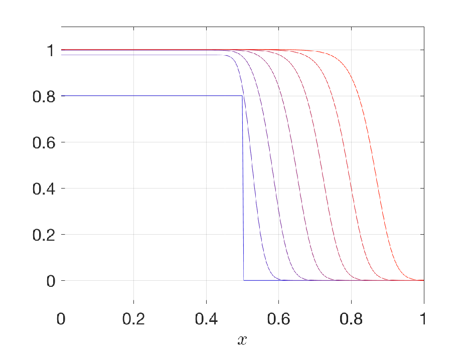
Figure 4 represents the discrete solutions with the same numerical parameters as in Figure 3 but with the initial datum $u_{0}(x)=1$ for $0<x<1/2$ and $u_{0}(x)=0$ else. Also in this example, the lower and upper bounds $0\leq\exp(\lambda_{h}^{k})\leq 1$ are always satisfied.

5.2. Entropy decay

Proposition 9 shows that the discrete entropy $S_{h}^{k}$ decays exponentially fast if $S_{h}^{0}<|\Omega|=1$ . To illustrate this behavior numerically, we consider the one-group model with initial condition $u_{0}(x)=1$ for $0<x<1/2$ and $u_{0}(x)=10^{-16}$ else. Figure 5 (left) shows that there are two different slopes. For small times, the entropy decay is rather slow. When the time step $k$ is sufficiently large such that $\exp(\lambda_{h}^{k})>\varepsilon$ for some $\varepsilon>0$ , the reaction dominates, and the entropy decay becomes faster. This behavior becomes even more apparent in the case of pure diffusion (i.e. without reaction terms), illustrated in Figure 5 (right). We remark that in this situation, the total mass is conserved numerically.

Figure 6 shows the entropy decay in semi-log scale for the initial data $u_{0}(x)=n$ for $0<x<1/n$ and $u_{0}(x)=10^{-16}$ else for $n=3,6,12$ . Then

S_{h}^{0}=\int_{0}^{\frac{1}{n}}(n\log(n)-n+1)dx+\int_{\frac{1}{n}}^{1}1dx=\log n

is larger than $|\Omega|=1$ if $n>e$ . We observe a region in which the decay rate is very small and it becomes smaller when $n$ (and $S_{h}^{0}$ ) increases. This indicates that the assumption $S_{0}^{h}<|\Omega|$ is not just technical to derive exponential time decay.

5.3. Traveling waves

We are looking for traveling-wave solutions to (37) with $D=1$ . Setting $u(x,t)=\phi(s)$ with $s=x-ct$ , the Fisher-KPP equation can be rewritten as a system of first-order differential equations:

(39)

\phi^{\prime}=-c\phi+\psi(\psi-1),\quad\psi^{\prime}=\phi,\quad t>0.

We choose the initial data $\phi(0)=1$ and $\psi(0)=-10^{-10}$ . The (reference) traveling-wave solution $\phi(s)$ , computed from (39) using the Matlab command ode45, is compared in Figure 7 with the DG solution $\exp(\lambda_{h}^{k})$ , computed from the DG scheme (8), and the continuous $P_{1}$ finite-element solution $u_{h}$ . The solutions are shown at the time instances $t=0$ , $t=T/6$ , $t=T/3$ , and $t=T/2$ (with $T=20$ ). Both approximations are diffusive, i.e., the traveling-wave speed is overestimated by the DG and finite-element solutions. On the finer mesh with $N_{\rm el}=80$ elements, the DG solution is clearly less diffusive compared to the other discrete solutions on the coarser mesh with $N_{\rm el}=50$ elements. Better approximations are expected by using a higher-order time discretization. Structure preservation of higher-order temporal approximations is a delicate topic (see, e.g., [21]) and will be studied in a future work. Also an error analysis is postponed to a future work.

Appendix A Linear elements: Existence of solutions for $\varepsilon=0$

We show that the regularization term $\varepsilon\int_{\Omega}\lambda_{h}^{k}\phi_{h}dx$ in the DG scheme (8) is not needed if we consider linear elements.

Proposition 15 (Existence for $p=1$ ).

Let $p=1$ , $\lambda_{h}^{k-1}\in V_{h}$ , and $S_{0}^{h}<|\Omega|$ . Then there exists a solution $\lambda_{h}^{k}\in V_{h}$ to (8) with $\varepsilon=0$ .

Proof.

The proof is based on the idea of the proof of [1, Lemma 3.10]. Let $\varepsilon>0$ and let $\lambda_{h}^{k}\in V_{h}$ be a solution to (8) given by Proposition 6. In order to emphasize the dependency on $\varepsilon$ , we write $\lambda_{\varepsilon}:=\lambda_{h}^{k}$ . Our goal is to derive an $\varepsilon$ -uniform $L^{\infty}(\Omega)$ bound for $\lambda_{\varepsilon}$ .

Step 1: We derive first some estimates for $e^{\lambda_{\varepsilon}}$ . Lemma 8 shows that

(40)

\delta\leq\int_{\Omega}e^{\lambda_{\varepsilon}}dx\leq M,

where $\delta=\sigma_{-}(S_{h}^{0}/|\Omega|)$ and $M=\sigma_{+}(S_{h}^{0}/|\Omega|)$ . Since we assumed that $S_{h}^{0}<|\Omega|$ , we have $\delta>0$ . Using the coercivity estimate (12), the inequality (17), and $e^{\lambda_{\varepsilon}}(e^{\lambda_{\varepsilon}}-1)\lambda_{\varepsilon}\geq 0$ , we find that

S_{h}^{k}+\frac{\triangle t}{2}\sum_{K\in\mathcal{T}_{h}}\int_{K}e^{\lambda_{\varepsilon}}|\nabla\lambda_{\varepsilon}|^{2}dx+\frac{\triangle t}{3}\sum_{f\in\mathcal{E}_{h}}\int_{f}\frac{p^{2}}{{\tt h}}\alpha(\lambda_{\varepsilon})|\ldbrack\lambda_{\varepsilon}\rdbrack|^{2}ds\leq S^{k-1}_{h}\leq S_{h}^{0},

where we used in the last step the monotonicity of $k\mapsto S_{h}^{k}$ , guaranteed by Lemma 7. Consequently,

(41)

\sum_{K\in\mathcal{T}_{h}}\int_{K}e^{\lambda_{\varepsilon}}|\nabla\lambda_{\varepsilon}|^{2}dx+\sum_{f\in\mathcal{E}_{h}}\int_{f}\frac{p^{2}}{{\tt h}}\alpha(\lambda_{\varepsilon})|\ldbrack\lambda_{\varepsilon}\rdbrack|^{2}ds\leq M^{\prime}:=\frac{3S_{h}^{0}}{\triangle t}.

Step 2: We claim that for any $\varepsilon>0$ , there exists an element $K_{\varepsilon}\in\mathcal{T}_{h}$ and a constant $\mu>0$ , independent of $\varepsilon$ , such that

(42)

\|\lambda_{\varepsilon}\|_{L^{\infty}(K_{\varepsilon})}\leq\mu.

For the proof, let $N\in{\mathbb{N}}$ be the number of elements in $\mathcal{T}_{h}$ . The lower and upper bounds (40) imply the existence of an element $K_{\varepsilon}\in\mathcal{T}_{h}$ such that

(43)

\frac{\delta}{N}\leq\int_{K_{\varepsilon}}e^{\lambda_{\varepsilon}}dx\leq M.

By the mean-value theorem, there exists $x_{\varepsilon}\in K_{\varepsilon}$ such that

e^{\lambda_{\varepsilon}(x_{\varepsilon})}=\frac{1}{|K_{\varepsilon}|}\int_{K_{\varepsilon}}e^{\lambda_{\varepsilon}(x)}dx.

Then (43) gives

|\lambda_{\varepsilon}(x_{\varepsilon})|=\bigg|\log\bigg(\frac{1}{|K_{\varepsilon}|}\int_{K_{\varepsilon}}e^{\lambda_{\varepsilon}(x)}dx\bigg)\bigg|\leq\max\bigg\{\bigg|\log\frac{M}{|K_{\varepsilon}|}\bigg|,\log\frac{\delta}{N|K_{\varepsilon}|}\bigg|\bigg\}.

Since $\lambda_{\varepsilon}$ is a polynomial of degree one on $K_{\varepsilon}$ , by assumption, its gradient is constant on $K_{\varepsilon}$ , and we deduce from (41) and (43) that

|\nabla\lambda_{\varepsilon}|^{2}=\frac{\int_{K_{\varepsilon}}e^{\lambda_{\varepsilon}}|\nabla\lambda_{\varepsilon}|^{2}dx}{\int_{K_{\varepsilon}}e^{\lambda_{\varepsilon}}dx}\leq\frac{M^{\prime}N}{\delta}\quad\mbox{on }K_{\varepsilon}.

Combining the last two estimates, it follows for $x\in K_{\varepsilon}$ that

	$\displaystyle\|\lambda_{\varepsilon}(x)\|$	$\displaystyle\leq\|\lambda_{\varepsilon}(x_{\varepsilon})\|+\|x-x_{\varepsilon}\|\int_{0}^{1}\|\nabla\lambda_{\varepsilon}(x\varepsilon+\theta(x-x_{\varepsilon})\|d\theta$
		$\displaystyle\leq\max\bigg\{\bigg\|\log\frac{M}{\|K_{\varepsilon}\|}\bigg\|,\log\frac{\delta}{N\|K_{\varepsilon}\|}\bigg\|\bigg\}+\frac{M^{\prime}N}{\delta}=:\mu,$

which shows the claim.

Step 3: We wish to prove a uniform $L^{\infty}$ bound for $\lambda_{\varepsilon}$ on the faces or edges of $K_{\varepsilon}$ . Let $\mu>0$ and $K_{\varepsilon}\in\mathcal{T}_{h}$ such that $\|\lambda_{\varepsilon}\|_{L^{\infty}(K_{\varepsilon})}\leq\mu$ . Set $K_{-}:=K_{\varepsilon}$ and consider neighboring elements $K_{+}\in\mathcal{T}_{h}$ satisfying $f\in\partial K_{-}\cap\partial K_{+}\neq\emptyset$ . Furthermore, let $\lambda_{\pm}=\lambda_{\varepsilon}|_{K_{\pm}}$ . We claim that there exists $C_{\mu}>0$ , independent of $\varepsilon$ , such that

(44)

\|\lambda_{+}\|_{L^{\infty}(f)}\leq C_{\mu}.

The idea is to prove an $L^{2}(f)$ estimate for $\lambda_{\varepsilon}$ , as the equivalence of all norms in the finite-dimensional setting then implies the desired $L^{\infty}(f)$ bound.

Observe that

\max\big\{(e^{\lambda_{\varepsilon}})_{-},(e^{\lambda_{\varepsilon}})_{+}\big\}\geq(e^{\lambda_{\varepsilon}})_{-}\geq\exp(-\|\lambda_{-}\|_{L^{\infty}(f)})\geq\exp(-\|\lambda_{-}\|_{L^{\infty}(K_{-})})\geq\exp(-\mu).

Then we can estimate the stabilization function $\alpha$ according to

\alpha(\lambda_{\varepsilon})\geq\frac{3}{2}C_{\rm inv}^{2}\exp(-\|\lambda_{-}\|_{L^{\infty}(K_{-})})^{2}\exp(\|\lambda_{-}\|_{L^{\infty}(K_{-})}\geq\frac{3}{2}C_{\rm inv}^{2}e^{-\mu}.

To estimate the $L^{2}(f)$ norm of $\lambda_{-}|_{f}$ , we use the inequality $|\lambda_{+}|\leq|\lambda_{+}-\lambda_{-}|+|\lambda_{-}|=|\ldbrack\lambda_{\varepsilon}\rdbrack|+|\lambda_{\varepsilon}|$ on $f$ . Then (42) yields

\int_{f}|\lambda_{+}|^{2}ds\leq 2\int_{f}\big(|\lambda_{\varepsilon}|^{2}+|\ldbrack\lambda_{\varepsilon}\rdbrack|^{2}\big)ds\leq 2|f|\mu^{2}+\frac{4e^{\mu}}{3C_{\rm inv}^{2}}\int_{f}\alpha(\lambda_{\varepsilon})|\ldbrack\lambda_{\varepsilon}\rdbrack|^{2}ds=:\beta_{\mu},

and $\beta_{\mu}$ is uniform in $\varepsilon$ (but not in $h$ ) in view of (41). We conclude that

\|\lambda_{\varepsilon}\|_{L^{\infty}(f)}\leq C\|\lambda_{\varepsilon}\|_{L^{2}(f)}\leq C\beta_{\mu}^{1/2}.

Step 4: Denote by $(\phi_{0},\ldots,\phi_{d})$ the basis of $P_{1}(K_{+})$ such that $\phi_{i}(e_{j})=\delta_{ij}$ for $i$ , $j=0,\ldots,d$ , where the vertices $e_{i}$ of $K_{+}$ are ordered in such a way that $e_{0}\not\in f$ . Then we can formulate $\lambda_{+}$ on $K_{+}$ as

\lambda_{+}(x)=\sum_{i=0}^{d}a_{i}^{\varepsilon}\phi_{i}(x),\quad x\in K_{+},

where $a_{i}^{\varepsilon}=\lambda_{+}(e_{i})$ . Estimate (44) shows that $\lambda_{+}(e_{i})$ is uniformly bounded at the vertices $a_{1},\ldots,a_{d}$ of $K_{+}$ , i.e. $|a_{i}^{\varepsilon}|\leq C_{\mu}$ for all $i=1,\ldots,d$ .

Step 5: We wish to estimate the remaining vertex $e_{0}^{\varepsilon}$ that is not an element of $K_{-}=K_{\varepsilon}$ . We claim that there exist constants $L_{\mu}\leq U_{\mu}$ , being independent of $\varepsilon$ , such that

L_{\mu}\leq a_{0}^{\varepsilon}\leq U_{\mu}.

We first prove the upper bound. Using the bound for $a_{i}^{\varepsilon}$ for $i=1,\ldots,d$ , we have

\lambda_{+}\geq a_{0}^{\varepsilon}\phi_{0}-\sum_{i=1}^{d}|a_{i}^{\varepsilon}||\phi_{i}|\geq a_{0}^{\varepsilon}\phi_{0}-C_{\mu}\sum_{i=1}^{d}|\phi_{i}|\geq a_{0}^{\varepsilon}\phi_{0}-C_{\mu}d.

If $a_{0}^{\varepsilon}\leq 0$ , there is nothing to show. Otherwise, it follows from (43) that

M\geq\int_{K_{+}}\exp(\lambda_{+})dx\geq\int_{K_{+}}\exp(a_{0}^{\varepsilon}\phi_{0}-C_{\mu}d)dx\geq e^{-C_{\mu}d}\int_{K_{+}}a_{0}^{\varepsilon}\phi_{0}dx.

Then, setting $c_{0}=\int_{K_{+}}\phi_{0}dx$ , we infer that $a_{0}^{\varepsilon}\leq Me^{C_{\mu}d}/c_{0}=:U_{\mu}$ .

The proof of the lower bound is more involved. Let $f_{0}$ be the face or edge that is opposite of the vertex $e_{0}$ , and let $f_{1},\ldots,f_{d}$ be the remaining faces or edges. For later use, we note that the integrals

	$\displaystyle I(b)$	$\displaystyle:=\int_{K_{+}}\bigg(\|b\nabla\phi\|+C_{\mu}\sum_{i=1}^{d}\|\nabla\phi_{i}\|\bigg)^{2}e^{b\phi_{0}+C_{\mu}d}dx,$
	$\displaystyle J(b)$	$\displaystyle:=\sum_{j=1}^{d}\int_{f_{j}}\bigg(\|b\nabla\phi\|+C_{\mu}\sum_{i=1}^{d}\|\nabla\phi_{i}\|\bigg)^{2}e^{b\phi_{0}+C_{\mu}d}dx$

converge to zero as $b\to-\infty$ , so there exists $L^{\prime}_{\mu}\in{\mathbb{R}}$ such that

(45)

I(b)+J(b)\leq 1\quad\mbox{for all }b\leq L^{\prime}_{\mu}.

We estimate

|\nabla\lambda_{+}\cdot n|\geq|a_{0}^{\varepsilon}||\nabla\phi_{0}\cdot n|-\sum_{i=1}^{d}|a_{i}^{\varepsilon}||\nabla\phi_{0}\cdot n|\geq|a_{0}^{\varepsilon}||\nabla\phi_{0}\cdot n|-C_{\mu}d\max_{i=1,\ldots,d}|\nabla\phi_{i}|.

As we assumed that $p=1$ , the expression $|\nabla\lambda_{\varepsilon}\cdot n|$ is constant. Thus, since $|\nabla\phi_{0}\cdot n|>0$ and $\lambda_{\varepsilon}\geq-C_{\mu}$ on $f_{0}$ , by (44), the previous inequality gives

	$\displaystyle\|a_{0}^{\varepsilon}\|$	$\displaystyle\leq\frac{1}{\|\nabla\phi_{0}\cdot n\|}\big(\|\nabla\lambda_{\varepsilon}\cdot n\|+C_{\mu}d\max_{i=1,\ldots,d}\|\nabla\phi_{i}\|\big)$
(46)			$\displaystyle\leq\frac{1}{\|\nabla\phi_{0}\cdot n\|}\bigg(\frac{e^{C_{\mu}}}{\|f_{0}\|}\bigg\|\int_{f_{0}}e^{\lambda_{\varepsilon}}\nabla\lambda_{\varepsilon}\cdot nds\bigg\|+C_{\mu}d\max_{i=1,\ldots,d}\|\nabla\phi_{i}\|\bigg).$

An integration by parts leads to

	$\displaystyle\int_{f_{0}}e^{\lambda_{\varepsilon}}\nabla\lambda_{\varepsilon}\cdot nds+\sum_{i=1}^{d}\int_{f_{i}}e^{\lambda_{\varepsilon}}\nabla\lambda_{\varepsilon}\cdot nds$	$\displaystyle=\int_{K_{+}}e^{\lambda_{\varepsilon}}\Delta\lambda_{\varepsilon}dx+\int_{K_{+}}e^{\lambda_{\varepsilon}}\|\nabla\lambda_{\varepsilon}\|^{2}dx$
		$\displaystyle=\int_{K_{+}}e^{\lambda_{\varepsilon}}\|\nabla\lambda_{\varepsilon}\|^{2}dx,$

since $\lambda_{\varepsilon}$ is linear on $K_{+}$ , so the Laplacian vanishes. Hence, using

\lambda_{+}\leq a_{0}^{\varepsilon}\phi_{0}+\sum_{i=1}^{d}|a_{i}^{\varepsilon}||\phi_{i}|\leq a_{0}^{\varepsilon}\phi_{0}+C_{\mu}d.

and (45), we have

\displaystyle\bigg|\int_{f_{0}}e^{\lambda_{\varepsilon}}\nabla\lambda_{\varepsilon}\cdot nds\bigg|\leq I(a_{0}^{\varepsilon})+J(a_{0}^{\varepsilon})\leq 1

if we choose $a_{0}^{\varepsilon}\leq L_{\mu}^{\prime}$ . Inserting this information into (46), it follows for all $a_{0}^{\varepsilon}\leq L_{\mu}^{\prime}$ that

|a_{0}^{\varepsilon}|\leq\frac{1}{|\nabla\phi_{0}\cdot n|}\bigg(\frac{e^{C_{\mu}}}{|f_{0}|}+C_{\mu}d\max_{i=1,\ldots,d}|\nabla\phi_{i}|\bigg)=:-L_{\mu}^{\prime\prime}.

Thus, setting $L_{\mu}=\min\{L_{\mu}^{\prime},L_{\mu}^{\prime\prime}\}$ , we conclude that $a_{0}^{\varepsilon}\geq L_{\mu}$ .

Step 6: Combining the previous steps, we infer that there exists a constant $g(\mu)>0$ such that

\|\lambda_{\varepsilon}\|_{L^{\infty}(K_{+})}\leq g(\mu).

This estimate means that if $\lambda_{\varepsilon}$ is bounded in some element with constant $\mu$ , then $\lambda_{\varepsilon}$ is bounded in the neighboring elements with constant $g(\mu)$ . Now, take an arbitrary element $K\in\mathcal{T}_{h}$ . Then there exists a finite sequence $K^{0},K^{1},\ldots,K^{m}$ of elements with $K^{0}=K_{\varepsilon}$ and $K^{m}=K$ such that $K^{j-1}$ and $K^{j}$ are neighboring elements. Repeating the arguments of Steps 3-5, the bound $\|\lambda_{\varepsilon}\|_{L^{\infty}(K^{1})}\leq\mu^{\prime}:=g(\mu)$ implies that $\|\lambda_{\varepsilon}\|_{L^{\infty}(K^{2})}\leq g(\mu^{\prime})=g(g(\mu))$ . Thus, by iteration,

\|\lambda_{\varepsilon}\|_{L^{\infty}(K)}\leq\underbrace{(g\circ\cdots\circ g)}_{\text{$m$ times}}(\mu).

The upper bound is independent of $\varepsilon$ and holds for all elements $K\in\mathcal{T}_{h}$ . Consequently, $(\lambda_{\varepsilon})$ is bounded in $L^{\infty}(\Omega)$ .

We deduce that there exists a subsequence (not relabeled) such that $\lambda_{\varepsilon}\to\lambda$ strongly in $L^{\infty}(\Omega)$ , recalling that $V_{h}$ is finite-dimensional. In fact, the convergence holds in any norm. Thus, we can pass to the limit $\varepsilon\to 0$ in (8), and the limit equation is the same as (8) with $\varepsilon=0$ . ∎

References

[1] A. Ait Hammou Oulhaj, C. Cancès, and C. Chainais-Hillairet. Numerical analysis of a nonlinearly stable and positive control volume finite element scheme for Richards equation with anisotropy. ESAIM: Math. Model. Numer. Anal. 52 (2018), 1533-1567.
[2] D. Arnold. An interior penalty finite element method for discontinuous elements. SIAM J. Numer. Anal. 19 (1982), 742-760.
[3] D. Arnold, F. Brezzi, B. Cockburn, and L. Marini. Unified analysis of discontinuous Galerkin methods for elliptic problems. SIAM J. Numer. Anal. 39 (2002), 1749-1779.
[4] A. Arnold, P. Markowich, G. Toscani, and A. Unterreiter. On generalized Csiszár-Kullback inequalities. Monatsh. Math. 131 (2000), 235-253.
[5] G. A. Baker. Finite element methods for elliptic equations using nonconforming elements. Math. Comput. 31 (1977), 45-59.
[6] H. Brézis. Functional Analysis, Sobolev Spaces and Partial Differential Equations. Springer, New York, 2011.
[7] A. Buffa and C. Ortner. Compact embeddings of broken Sobolev spaces and applications. IMA J. Numer. Anal. 29 (2009), 827-855.
[8] M. Burger, M. Di Francesco, J.-F. Pietschmann, and B. Schlake. Nonlinear cross-diffusion with size exclusion. SIAM J. Math. Anal. 42 (2010), 2842-2871.
[9] F. Cavalli, G. Naldi, and I. Perugia. Discontinuous Galerkin approximation of relaxation models for linear and nonlinear diffusion equations. SIAM J. Sci. Comput. 34 (2012), A105-A136.
[10] P. Ciarlet (ed.). The Finite Element Method for Elliptic Problems. Studies Math. Appl., volume 4, pp. 1-530. North-Holland, Amsterdam, 1978.
[11] I. Ekeland and R. Teman. Convex Analysis and Variational Problems. North-Holland, Amsterdam, 1972.
[12] R. A. Fisher. The wave of advance of advantageous genes. Ann. Eugenics 7 (1937), 353-369.
[13] H. Gajewski. On existence, uniqueness and asymptotic behavior of solutions of the basic equations for carrier transport in semiconductors. Z. Angew. Math. Mech. 65 (1985), 101-108.
[14] G. Gassner, A. Winters, and D. Kopriva. Split form nodal discontinuous Galerkin schemes with summation-by-parts property for the compressible Euler equations. J. Comput. Phys. 327 (2016), 39-66.
[15] L. Guo and Y. Yang. Positivity preserving high-order local discontinuous Galerkin method for parabolic equations with blow-up solutions. J. Comput. Phys. 289 (2015), 181-195.
[16] E. Hairer, C. Lubich, and G. Wanner. Geometric Numerical Integration. Springer, Berlin, 2006.
[17] S. Hasnain, M. Saqib, and D. Suleiman Mashat. Numerical study of one dimensional Fishers KPP equation with finite difference schemes. Amer. J. Comput. Math. 7 (2017), 70-83.
[18] P. Houston, C. Schwab, and E. Süli. Discontinuous $hp$ -finite element methods for advection-diffusion-reaction problems. SIAM J. Numer. Anal. 39 (2002), 2133-2163.
[19] A. M. Il’in. A difference scheme for a differential equation with a small parameter multiplying the highest derivative. Mat. Zametki 6 (1969), 237-248.
[20] A. Jüngel. Entropy Methods for Diffusive Partial Differential Equations. BCAM Springer Briefs, Springer, 2016.
[21] A. Jüngel and S. Schuchnigg. Entropy-dissipating semi-discrete Runge-Kutta schemes for nonlinear diffusion equations. Commun. Math. Sci. 15 (2017), 27-53.
[22] P. Lesaint and P. A. Raviart. On a finite element method for solving the neutron transport equation. In: C. de Boor (ed.). Mathematical Aspects of Finite Elements in Partial Differential Equations, pp. 89-123. Academic Press, New York, 1974.
[23] H.-L. Liu and Z. Wang. An entropy satisfying discontinuous Galerkin method for nonlinear Fokker-Planck equations. J. Sci. Comput. 68 (2016), 1217-1240.
[24] J. Macías-Díaz, S. Jerez-Galiano, and A. Puri. An explicit positivity-preserving finite-difference scheme for the classical Fisher-Kolmogorov-Petrovsky-Piscounov equation. Appl. Math. Comput. 9 (2012), 5829-5839.
[25] V. Maz’ya and J. Rossmann. Elliptic Equations in Polyhedral Domains. American Mathematical Society, Providence, 2010.
[26] P.-A. Meyer. Probability and Potentials. Blaisdell Publishing, Toronto, 1966.
[27] J. Nitsche. Über ein Variationsprinzip zur Lösung von Dirichlet-Problemen bei Verwendung von Teilräumen, die keinen Randbedingungen unterworfen sind. Abh. Math. Sem. Univ. Hamburg 36 (1971), 9-15.
[28] M. Parsani, M. Carpenter, T. Fisher, and E. Nielsen. Entropy stable staggered grid discontinuous spectral collocation methods of any order for the compressible Navier-Stokes equations. SIAM J. Sci. Comput. 38 (2016), A3129-A3162.
[29] P. Percell and M. Wheeler. A local residual finite element procedure for elliptic problems. SIAM J. Numer. Anal. 15 (1978), 705-714.
[30] S. Prudhomme, F. Pascal, J. T. Oden, and A. Romkes. Review of a priori error estimation for discontinuous Galerkin methods. TICAM REPORT 00-27, Texas Institute for Computational and Applied Mathematics, Austin, USA, 2000.
[31] W. Reed and T. Hill. Triangular mesh methods for the neutron transport equation. Proceedings of the American Nuclear Society for the conference “National topical meeting on mathematical models and computational techniques for analysis of nuclear systems”, Ann Arbor, Michigan, USA, 1973, 22 pages.
[32] B. Rivière, M. Wheeler, and Girault. A priori error estimates for finite element methods based on discontinuous approximation spaces for elliptic problems. SIAM J. Numer. Anal. 39 (2001), 902-931.
[33] Z. Sun, J. A. Carrillo, and C.-W. Shu. A discontinuous Galerkin method for nonlinear parabolic equations and gradient flow problems with interaction potentials. J. Comput. Phys. 352 (2018), 76-104.
[34] M. Wheeler. An elliptic collocation-finite element method with interior penalties. SIAM J. Numer. Anal. 15 (1978), 152-161.
[35] O. P. Yadav and R. Jiwari. Finite element analysis and approximation of Burgers-Fisher equation. Numer. Meth. Part. Diff. Eqs. 33 (2017), 1652-1677.
[36] R. Zhang, J. Zhu, Jiang, A. Loula, F. D. Abimael, and X. Yu. Operator splitting combined with positivity-preserving discontinuous Galerkin method for the chemotaxis model. J. Comput. Appl. Math. 302 (2016), 312-326.

(6)		$\displaystyle\\|\xi\\|_{L^{2}(\partial K)}$	$\displaystyle\leq C_{\rm inv}\frac{p}{\sqrt{h_{K}}}\\|\xi\\|_{L^{2}(K)},$
	$\displaystyle\\|\nabla\xi\cdot n_{f}\\|_{L^{2}(\partial K)}$	$\displaystyle\leq C_{\rm inv}\frac{p}{\sqrt{h_{K}}}\\|\nabla\xi\\|_{L^{2}(K)}.$

	$\displaystyle\sum_{f\in\mathcal{E}_{h}}\int_{f}\beta_{f}^{2}\{e^{v}\nabla v\}^{2}ds$	$\displaystyle=\frac{1}{4}\sum_{f\in\mathcal{E}_{h}}\int_{f}\beta_{f}^{2}\big\|(e^{v}\nabla v)_{-}+(e^{v}\nabla v)_{+}\big\|^{2}ds$
		$\displaystyle\leq\frac{1}{2}\sum_{f\in\mathcal{E}_{h}}\int_{f}\beta_{f}^{2}\big(\|(e^{v}\nabla v)_{-}\|^{2}+\|(e^{v}\nabla v)_{+}\|^{2}\big)ds$
		$\displaystyle=\frac{1}{2}\sum_{f\in\mathcal{E}_{h}}\int_{f}\beta_{f}^{2}\big(\max\{(e^{v})_{-},(e^{v})_{+}\}\big)^{2}\big(\|(\nabla v)_{-}\|^{2}+\|(\nabla v)_{+}\|^{2}\big)ds.$

	$\displaystyle\sum_{f\in\mathcal{E}_{h}}\int_{f}\beta_{f}^{2}\{e^{v}\nabla v\}^{2}ds$	$\displaystyle\leq\frac{1}{2}\sum_{K\in\mathcal{T}_{h}}\int_{\partial K}\gamma_{K}^{2}\|\nabla v\|^{2}ds\leq\frac{1}{2}C_{\rm inv}^{2}\sum_{K\in\mathcal{T}_{h}}\gamma_{K}^{2}\frac{p^{2}}{h_{K}}\int_{K}\|\nabla v\|^{2}dx$
		$\displaystyle\leq\frac{1}{2}C_{\rm inv}^{2}p^{2}\sum_{K\in\mathcal{T}_{h}}\frac{\gamma_{K}^{2}}{h_{K}}\exp(\\|v\\|_{L^{\infty}(K)})\int_{K}e^{v}\|\nabla v\|^{2}dx$
		$\displaystyle=\frac{1}{2}\sum_{K\in\mathcal{T}_{h}}\int_{K}e^{v}\|\nabla v\|^{2}dx.$

	$\displaystyle\frac{p^{2}}{{\tt h}}\alpha(v)-\frac{1}{\beta_{f}^{2}}$	$\displaystyle\geq\frac{3}{2}\frac{p^{2}}{{\tt h}}C_{\rm inv}^{2}\big(\max\{(e^{v})_{-},(e^{v})_{+}\}\big)^{2}\max\big\{\exp(\\|v\\|_{L^{\infty}(K_{-})}),\exp(\\|v\\|_{L^{\infty}(K_{+})})\big\}$
		$\displaystyle\phantom{xx}{}-\frac{C_{\rm inv}^{2}p^{2}(\max\{(e^{v})_{-},(e^{v})_{+}\})^{2}}{\min\{h_{K_{-}}\exp(-\\|v\\|_{L^{\infty}(K_{-})}),h_{K_{+}}\exp(-\\|v\\|_{L^{\infty}(K_{+})})\}}$
		$\displaystyle\geq\frac{p^{2}}{2{\tt h}}C_{\rm inv}^{2}(\max\{(e^{v})_{-},(e^{v})_{+}\})^{2}\max\big\{\exp(\\|v\\|_{L^{\infty}(K_{-})}),\exp(\\|v\\|_{L^{\infty}(K_{+})})\big\}$
		$\displaystyle=\frac{1}{3}\frac{p^{2}}{{\tt h}}\alpha(v).$

	$\displaystyle\triangle t\\|e^{\lambda_{h}^{k}/2}\\|_{\rm DG}^{2}$	$\displaystyle\leq\triangle t\int_{\Omega}(2+s(e^{\lambda_{h}^{k}}))dx+\frac{1}{2\min\{1,C_{\rm inv}^{2}\}}\int_{\Omega}\big(s(e^{\lambda_{h}^{k-1}})-s(e^{\lambda_{h}^{k}})\big)dx$
		$\displaystyle=2\triangle t\|\Omega\|+\bigg(\triangle t-\frac{1}{2\min\{1,C_{\rm inv}^{2}\}}\bigg)S_{h}^{k}+\frac{S_{h}^{k-1}}{2\min\{1,C_{\rm inv}^{2}\}}$
		$\displaystyle\leq 2\triangle t\|\Omega\|+\bigg(\triangle t-\frac{1}{2\min\{1,C_{\rm inv}^{2}\}}\bigg)S_{h}^{k}+\frac{S_{h}^{0}}{2\min\{1,C_{\rm inv}^{2}\}}.$

Abstract.

Key words and phrases:

2000 Mathematics Subject Classification

1. Introduction

2. Notation and auxiliary results

Lemma 1 (Inverse trace inequality; Lemma 2.1 in [32]).

Lemma 2 (Multiplicative trace inequality; Lemma A.2 in [30]).

Lemma 3 (Discrete Poincaré-Wirtinger inequality; Theorem 4.1 in [7]).

Lemma 4 (DG compact embedding; Lemma 8 in [7]).

3. Analysis of the DG scheme: existence and structure preservation

3.1. Existence of a discrete solution

Lemma 5 (Coercivity of BB).

Proof.

Proposition 6 (Existence).

Proof.

3.2. Discrete entropy inequality and exponential decay

Lemma 7 (Discrete entropy inequality).

Proof.

Lemma 8 (Bounds for the total mass).

Proof of Lemma 8.

Proposition 9 (Discrete entropy decay).

Lemma 10.

Proof.

Proof of Proposition 9.

Theorem 11 (Decay in the L1​(Ω)L^{1}(\Omega) norm).

Proof.

Remark 12.

4. Analysis of the DG scheme: numerical convergence

Lemma 13 (Uniform bound in DG norm).

Proof.

Theorem 14 (Convergence).

Proof.

5. Numerical results

5.1. One group of species

5.2. Entropy decay

5.3. Traveling waves

Appendix A Linear elements: Existence of solutions for ε=0\varepsilon=0

Proposition 15 (Existence for p=1p=1).

Proof.

References

Lemma 5 (Coercivity of $B$ ).

Theorem 11 (Decay in the $L^{1}(\Omega)$ norm).

Appendix A Linear elements: Existence of solutions for $\varepsilon=0$

Proposition 15 (Existence for $p=1$ ).