Partial Order Pruning: for Best Speed/Accuracy Trade-off in
Neural Architecture Search
Abstract
Achieving good speed and accuracy trade-off on a target platform is very important in deploying deep neural networks in real world scenarios. However, most existing automatic architecture search approaches only concentrate on high performance. In this work, we propose an algorithm that can offer better speed/accuracy trade-off of searched networks, which is termed “Partial Order Pruning”. It prunes the architecture search space with a partial order assumption to automatically search for the architectures with the best speed and accuracy trade-off. Our algorithm explicitly takes profile information about the inference speed on the target platform into consideration. With the proposed algorithm, we present several Dongfeng (DF) networks that provide high accuracy and fast inference speed on various application GPU platforms. By further searching decoder architectures, our DF-Seg real-time segmentation networks yield state-of-the-art speed/accuracy trade-off on both the target embedded device and the high-end GPU.
1 Introduction
Deploying deep convolutional neural networks (CNNs) on real-world embedded devices is attracting increasing research interest. Different from high-end GPUs, these devices usually offer rather limited computation capacity, leading to low efficiency when deploying popular high accuracy CNN models he2016deep; chen2018deeplab on them. Despite the considerable efforts on accelerating inference of CNNs such as pruning guo2016dynamic, quantization wu2016quantized and factorization liu2015sparse, fast inference speed11 1 Inference speed is measured by inference latency, which is defined as inference time with batch size 1 in a CNN. is usually achieved at the cost of degraded performance paszke2016enet; krizhevsky2012imagenet. In this paper, we address such a practical problem: Given a target platform, what is the best speed/accuracy trade-off boundary curve by varying CNN architecture? Or more specifically, we aim to answer two questions: 1) Given the maximum acceptable latency, what is the best accuracy one can get? 2) To meet certain accuracy requirements, what is the lowest inference latency one can expect?

Some existing works manually design high accuracy network architectures zhao2018icnet; yu2018bisenet; howard2017mobilenets; sandler2018inverted. They usually adopt an indirect metric, i.e. FLOP, to estimate the network complexity, but the FLOP count does not truly reveal the actual inference speed. For example, for a convolution on Nvidia GPUs which is highly optimized in terms of both hardware and software design lavin2016fast, one can assume it is times slower than a convolution on GPUs since it has times more FLOPs, which is not true actually. Besides, another important factor that affects the inference speed, the memory access, is not covered by measuring FLOPs. Considering the diversities of hardware and software, it is almost impossible to find one single architecture that is optimal for all the platforms.
Some other works attempt to automatically search for the optimal network architecture zoph2018learning; real2018regularized; darts, but they also rely on FLOPs to estimate the network complexity and do not take into account the discrepancy of this metric with the actual inference speed and also the target platforms. Despite a few works dong2018dpp; cai2018proxylessnas; fbnet consider the actual inference speed on target platforms, they search the architecture in each individual building block and keep fixed the overall architecture, i.e. depth and width.
In this paper, we develop an efficient architecture search algorithm that automatically selects the networks that offer better speed/accuracy trade-off on a target platform. The proposed algorithm is termed “Partial Order Pruning”, with which some candidates that fail to give better speed/accuracy trade-off are filtered out at early stages of the architecture searching process based on a partial order assumption (see Section 3.3 for details). For example, a wider network cannot be more efficient than a narrower one with the same depth, thus accordingly some wider ones are discarded. By pruning the search space in this way, our algorithm is forced to concentrate on those architectures that are more likely to lift the boundary of speed/accuracy trade-off.
The proposed “Partial Order Pruning” algorithm differs from previous neural architecture search algorithms in three aspects. Firstly, it explicitly takes platform characteristics into consideration. Secondly, it balances the width and depth of the overall architecture, instead of searching for complicated building blocks. Thirdly, it employs a partial order assumption and a cutting plane algorithm to accelerate searching, instead of using reinforcement learning, evolutionary algorithms or gradient-based algorithms.
With the proposed algorithm, we are able to obtain a set of networks that provide better accuracy and faster inference speed on a target platform, which we call Dongfeng (DF) networks. We apply our algorithm to searching decoder architectures in semantic segmentation and gain a set of DF-Seg networks. Figure 1 shows a comparison of our DF-Seg networks and other methods. It can be seen that our segmentation networks achieve new state-of-the-art in real-time urban scene parsing tasks.
To sum up, we make following contributions to network architecture search:
- •
We are among the first to investigate the problem of balancing speed and accuracy of network architectures for network architecture search. By pruning the search space with a partial order assumption, our “Partial Order Pruning” algorithm can efficiently lift the boundary of speed/accuracy trade-off.
- •
We present several DF networks that provide both high accuracy and fast inference speed on target embedded device TX2. The accuracy of our DF1/DF2A networks exceeds ResNet18/50 on ImageNet validation set, but the inference latency is and lower, respectively.
- •
We apply the proposed algorithm to searching decoder architectures for a segmentation network. Together with DF backbone networks, we achieve new state-of-the-art in real-time segmentation on both high-end GPUs and target embedded device TX2. On GTX 1080Ti, our DF1-Seg network achieves FPS at resolution with . On TX2, our DF1-Seg network achieves FPS at resolution , i.e. 720p.
2 Related Work
Efficient Network Design
Group convolution plays a key role in current efficient CNN architecture design ma2018shufflenet; howard2017mobilenets; sandler2018inverted. MobileNet_V2 sandler2018inverted adopts an inverted residual module that uses group convolutions to reduce the FLOPs during inference. ShuffleNet zhang2018shufflenet uses pointwise group convolution and channel shuffle operation to reduce FLOPs while maintaining accuracy. ma2018shufflenet points out that there is a discrepancy between indirect metric (FLOPs) and direct metric (inference speed), and proposes four guidelines for efficient network design. These works design a single architecture without considering the target platform while our algorithm explicitly takes platform characteristics into consideration.

Neural Architecture Search
Automatic network architecture search is often tackled with either reinforcement learning zoph2018learning; zoph2017neural or evolutionary algorithms real2018regularized; real2017large. They require huge computational resources, and the obtained networks are relatively slower than manually designed ones ma2018shufflenet; dong2018dpp, even with comparable FLOPs. More recently, several gradient-based algorithms darts; fbnet; cai2018proxylessnas; dong2019search are proposed to reduce the architecture search cost. Besides, a few works dong2018dpp; fbnet; cai2018proxylessnas also take platform-related objectives into consideration in architecture search. Although their goal is somewhat similar to ours, our work differs in that we pursue the balance of width and depth of a network, instead of searching the architecture in each individual block.
Real-time Semantic Segmentation
Most semantic segmentation methods zhao2017pyramid; chen2018searching; chen2018encoder aim at high performance but with relatively slow inference speed. For fast semantic segmentation, early works paszke2016enet; badrinarayanan2017segnet employ relatively shallower backbone networks and lower image resolution, offering fast inference speed but poorer accuracy. More recently, ICNet zhao2018icnet uses the image cascade to speed up inference, in which pre-trained deep CNNs are only applied to the images with lowest resolution. BiSeNet yu2018bisenet employs a context path to obtain a sufficient receptive field, and an additional spatial path with a small stride to preserve spatial information. None of them attempts to accelerate inference by improving the backbone network, or considers the characteristics of target platforms. Comparatively, our algorithm explicitly takes platform characteristics into consideration, and aims at better speed/accuracy trade-off in both backbone network and decoder network.
Model Acceleration
Some researchers try to accelerate inference of a pre-trained network via quantization wu2016quantized, pruning guo2016dynamic, factorization liu2015sparse, etc. For example, NetAdapt yang2018netadapt automatically adapts a pre-trained CNN to a mobile platform given a resource budget. Compared with them, we try to balance the width and depth of the overall architecture.
3 Partial Order Pruning
3.1 Search Space
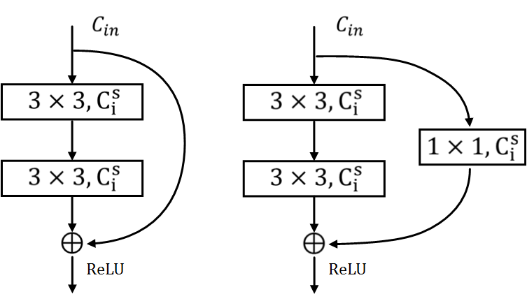
We provide a general network architecture in our search space, as shown in Figure 2. It consists of 6 stages to perform classification from input images. Stages 15 down-sample the spatial resolution of the input tensor with a stride of 2, and stage 6 produces the final prediction with a global average pooling and a fully connected layer. Stages extract common low-level features on large tensor size, which brings heavy computation burden. In pursuit of an efficient network, we only use one convolution layer in stage 1&2, i.e. and . We empirically find this is enough for achieving good accuracy. For stages 3, 4, 5, each consists of L, M, N residual blocks, where L, M ,N are integers, i.e. . Different settings of L/M/N lead to different network depths. The width (number of channels) of the -th residual block in stage is denoted as . Therefore, an architecture can be encoded as shown in Figure 2. In practice, we restrict . We empirically restrict the width of a block to be no narrower than its preceding blocks. Throughout this paper, we use the basic residual block proposed in he2016deep if not mentioned otherwise. As shown in Figure 2, the building block consists of two convolution layers and a shortcut connection. An additional projection layer is added if the size of input does not match the output tensor. All convolutional layers are followed with a batch normalization ioffe2015batch layer and ReLU nonlinearity.


3.2 Latency Estimation
The set of all possible architectures, with different depths (number of blocks) and widths (number of channels per block), is denoted as and usually referred to as the search space in neural architecture search darts; zoph2018learning. The latency of architectures in can vary from very small to positive infinity. But we only care about architectures in a subspace , which provide latency in the range .
We employ the profiler provided by TensorRT library to obtain layer-wise latency of a network. We empirically find that a block with a specific configuration (i.e. input/output tensor size) always consumes the same latency. Thus we can construct a look-up table providing latency of each block configuration, where is the number of channels in input/output tensor, and is the corresponding spatial size. For example, ms on TX2. By simply summing up the latency of all blocks, we can efficiently estimate the latency of an architecture . In Figure 3, we compare the estimated latency with the profiled latency. It shows our latency estimation is highly close to the actual profiled latency. All architectures with latency ranging form the subspace . This subspace construction significantly narrows down our search space, and hence accelerates the architecture selection.
3.3 Partial Order Assumption
A partial order is a binary relation defined over a set. It means that for certain pairs of elements in the set, one of the elements precedes the other in the ordering, denoted with . Here “partial” indicates that not every pair of elements needs to be comparable.

We find that there is a partial order relation among architectures in our search space. In Figure 4, we follow the architecture encoding in Figure 2, and illustrate the partial order relation among architectures. As explained in Section 3.2, is a set that contains all architectures in which we are interested. Let denote two elements in the set . If is shallower than but they are with the same width, or narrower than with same depth, we can borrow the concept from the order theory, and say that precedes in the ordering, denoted as . In the rest of this paper, we also call a precedent of if . Let and denote the accuracy and latency of the architecture . Then the partial order assumption of architectures can be summarized as
| (1) |
where . Formula (1) assumes that the latency and accuracy of an architecture are both higher than those of its precedents. This assumption may not hold for very deep networks that contain hundreds of layers he2016deep, but it is generally true for the efficient architectures of our concern, i.e. , which is experimentally verified in this work. We find all comparable architecture pairs in our trained architectures (Section 4.2), and compute the latency difference and accuracy difference in each pair. As shown in Figure 3, most points locate in the first quartile. This means the accuracy of the precedent is lower, for almost all comparable pairs. We also notice that a few points locate in the second quartile, but the lower limit of is , which is negligible considering the randomness during training. The above experimental results validate the reasonableness of our partial order assumption. This assumption can be utilized to prune the architecture search space, and speed up the search process significantly.
3.4 Partial Order Pruning
Formally, the goal of our architecture searching algorithm is to obtain an architecture with highest accuracy within every small latency range :
| (2) |
where is a short time period such as 0.1ms. Instead of searching at every small latency range, we optimize within the entire latency range . With our “Partial Order Pruning” algorithm, architecture searching at higher latency helps reduce the searching space at lower latency, and hence speeds up the overall searching process.

We use a cutting plane algorithm to optimize the combinational optimization problem in Formula (2). Algorithm 1 summarizes the pipeline of our algorithm. is a set containing all trained architectures, and is initialized as empty. denotes the search space pruned from . Each time we train a new architecture and obtain its accuracy , we are able to update the pruned search space . Figure 5 shows how to construct with the aforementioned partial order assumption. For each trained architecture , we find the fastest architecture that provides better accuracy:
| (3) |
If no is found that satisfies the condition, we continue to process the next . Let denote the precedents of with latency higher than , i.e.
| (4) |
Based on the partial order assumption, a precedent has lower latency and accuracy, i.e. . Therefore, even though we do not actually train , we can assume
| (5) |
In Figure 5, for all , , the shall locate in the corresponding shadow area. These architectures in are very unlikely to provide better speed/accuracy trade-off, and thus get pruned from the search space to avoid unnecessary training cost.
Given trained architectures , denotes the architectures that provide best speed/accuracy trade-off in trained architectures:
| (6) | |||||
Architectures in form the boundary for speed/accuracy trade-off we can achieve on the target platform. Figure 5 shows and the corresponding speed/accuracy trade-off boundary. Intuitively, no architecture in could obtain higher accuracy with lower latency. By pruning from the search space , our algorithm speeds up the architecture search process, and lifts the boundary of speed/accuracy trade-off. We stop the search process if no change to the happens for several iterations.
3.5 Decoder Design
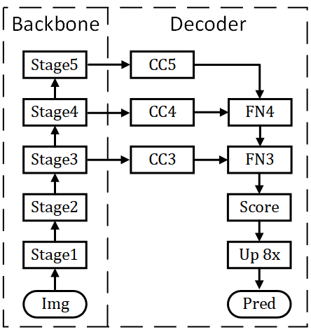
With the proposed Algorithm 1, we are able to find backbone architectures that provide best speed/accuracy trade-off on the target platform. Given a backbone network, we build semantic segmentation networks as shown in Figure 6. Each stage in the backbone network down-samples the resolution by 2. The resolution of tensors in stage 5 is thus of the input image. We append a pyramid pooling module zhao2017pyramid after the output tensor of stage 5 to improve segmentation performance. These tensors are then processed by the decoder to produce final prediction.
We append a convolution layer after stage 3/4/5 as a “Channel Controller” (CC). The channel controllers reduce the number of channels in the corresponding stage without changing its spatial resolution. The decoder fuses the tensors in different stages through the fusion nodes. The architecture of the fusion node is shown in Figure 6. A fusion node first projects a low resolution tensor from channels to channels with a convolution layer, and then up-samples it by 2. We concatenate the up-sampled tensor with a higher resolution tensor, and then process it with a convolution layer, to fuse the expressive power of different backbone stages. We fuse the features from stage 3/4/5 and produce a resolution score map. The score map is then up-sampled by 8 to produce final per-pixel semantic segmentation prediction.
Let , denote the width of each CC. We heuristically set , where is the number of classes. Given a backbone network, different settings of channel controllers, i.e. , lead to different decoder architectures. All the possible decoder CC settings form the search space of the decoder architecture. Similar to backbone network architectures, we also apply a partial order assumption over the CC settings. That is, a narrower decoder is always more efficient and less accurate than a wider one. Therefore we can also employ the “Partial Order Pruning” algorithm to lift the speed/accuracy trade-off boundary in the decoder architecture search.

4 Experiment
4.1 Experimental Settings
We adopt two typical kinds of hardware that provide different computational power.
- •
Embedded device: We use Nvidia Jetson TX2 with an integrated 256-core Pascal GPU as the target embedded device. It provides considerable computational power with limited electrical power consumption.
- •
High-end GPU: We use Nvidia Geforce GTX 1080Ti that provides enormous computing power. We also use GTX Titan X (Maxwell) for fair comparison with previous methods.
We adopt two tools to measure inference speed. First, we employ the widely used high-performance CNN inference framework TensorRT-3.0.4. Second, for a fair comparison with ICNet zhao2018icnet, we use the time measure tool Caffe Time, and set the repeating number to and take the average inference time for comparison. All experiments are performed under CUDA 9.0 and CUDNN V7.
We conduct experiments on two benchmark datasets. The ImageNet deng2009imagenet is a large-scale image classification dataset, which contains over 1.2 million color images in the training set and 50k color images in the validation set. The Cityscapes cordts2016cityscapes is a large benchmark dataset for urban scene parsing. It contains images with high quality pixel-level annotations, and is split to for training, for validation, and for testing.

4.2 Backbone Architecture Search
In contrast to current architecture search algorithms that conduct architecture searching on small datasets, we directly conduct architecture searching on ImageNet. We use the SGD optimizer with the poly learning rate policy to train models. The power is set to , and the momentum is set to . We use a weight decay of . The batch size is set to . We employ random scaling and stretching for data augmentation to relieve overfitting. Following goyal2017accurate, we first train each network for epochs with learning rate as a warm up scheme, and then train for epochs with an initial learning rate .
We conduct backbone architecture searching experiments on TX2 platform. During searching, we evaluate the single crop Top-1 accuracy on ImageNet validation set and the inference latency at resolution . We are interested in the efficient architectures with latency falling in the range , and construct the search space accordingly (Section 3.2). We conduct architecture search with Algorithm 1, and stop the search process when no remarkable boundary update is found during the search. The resulting speed/accuracy trade-off boundary is considered to be nearly optimal in our search space on the target platform TX2. We train networks in total, as shown in Figure 7. With the training configuration kept unchanged during architecture search, we train two representative network architectures with additional supervision szegedy2015going and more epochs, to further improve their accuracy. The resulting models are referred to as DF1, DF2. We further replace some of the building blocks in DF2 from basic block in Figure 2 to bottleneck block he2016deep. The resulting network is denoted as DF2A. Figure 7 and Table 1 give a comparison of our DF networks and popular models22 2 We report latency with our re-implementation. on the target platform TX2. Table 2 shows detailed architectures of these three DF networks. Training with more sophisticated methods, e.g. dropout or label smoothing, may produce higher accuracy, which however is not the focus of this paper.
| Model | Top1 Acc. | Latency (ms) | FLOPs |
|---|---|---|---|
| ShuffleNet_V2 ma2018shufflenet | 69.4% | 4.1 | 146M |
| ResNet-18 he2016deep | 69.0% | 4.4 | 1.8G |
| ShuffleNet_V1 zhang2018shufflenet | 67.4% | 4.7 | 140M |
| GoogLeNet szegedy2015going | 68.7% | 5.1 | 1.43G |
| MobileNet_V1 howard2017mobilenets | 70.8% | 6.1 | 569M |
| MobileNet_V2 sandler2018inverted | 71.9% | 8.7 | 300M |
| ResNet-50 he2016deep | 75.3% | 10.6 | 3.8G |
| FBNet-A fbnet | 73.0% | 5.9 | 249M |
| ProxylessNAS-GPU cai2018proxylessnas | 75.1% | 9.3 | - |
| NASNet-A zoph2018learning | 74.0% | 20.7 | 564M |
| PNASNET-5 liu2018progressive | 74.2% | 27.6 | 588M |
| DF1 | 69.8% | 2.5 | 746M |
| DF2 | 73.9% | 5.0 | 1.77G |
| DF2A | 76.0% | 6.5 | 1.97G |
| Stage | Layer | Output size | DF1 | DF2 | DF2A |
|---|---|---|---|---|---|
| 1 | Conv1 | ||||
| 2 | Conv2 | ||||
| 3 | Res3_x | ||||
| 4 | Res4_x | ||||
| 5 | Res5_x | ||||
| 6 | FC | Global Average Pooling, 1000-d FC, Softmax. | |||
| Depth | |||||
Compared with ResNet-18 and GoogLeNet, our DF1 obtains a higher accuracy but the inference latency is , lower than two baselines respectively. our DF2 has a similar latency but the accuracy is and higher than the baselines respectively. Furthermore, DF2A achieves a surpassing ResNet-50-level accuracy with a lower latency. Note we use the same building blocks with ResNet-18/50. So we attribute the better speed/accuracy trade-off to the better balancing between depth and width in our architectures. Specifically, our DF1/DF2A are slimmer and deeper than ResNet-18/50 for obtaining the same accuracy.
MobileNet howard2017mobilenets; sandler2018inverted and ShuffleNet zhang2018shufflenet; ma2018shufflenet are state-of-the-art efficient networks that are designed for mobile applications. We also compare our DF networks to them on TX2 in Table 1 and Figure 7. It can be seen our DF1 achieves higher accuracy but lower inference latency. The MobileNet/ShuffleNet have less FLOPs but higher latency. This is because they have higher memory access cost. The total memory cost (i.e. intermediate features) for ShuffleNet_V2 and DF1 is 4.86 and 2.91 respectively. This also indicates the FLOPs may be inconsistent with latency on the target platform wang2018pelee; ma2018shufflenet. Therefore, taking characteristics of target platform into consideration is necessary for achieving the best speed/accuracy trade-off.
We also compare our DF networks with other models searched by NAS methods zoph2018learning; liu2018progressive; fbnet; cai2018proxylessnas. As shown in Table 1, NASNet zoph2018learning and PNASNet liu2018progressive have not taken latency into consideration, leading to higher latency. Comparing to FBNet fbnet and ProxylessNAS cai2018proxylessnas, which also take target platform-related objectives into neural architecture search, our DF networks show better speed/accuracy trade-off. This can be explained as (a) DF networks are specifically searched for TX2 platform; (b) FBNet and ProxylessNAS use an inverted bottleneck module, which brings more memory access cost; (c) FBNet and ProxylessNAS aim at searching for better building block architectures while we balance the width and depth of the overall architecture.
We then discuss the search efficiency of our proposed algorithm. Figure 8 shows the number of pruned architectures in the search process. We prune architectures after training architectures.Therefore, our POP algorithm accelerates the architecture search process for times. Each model takes hours on a server with 8-GPUs. Training architectures takes GPU days in total. The computational cost of our architecture for searching on ImageNet is lower than the building block architecture searching zoph2018learning; real2018regularized on CIFAR-10 by an order.


Based on our architecture search results, we make following observations. 1) Very quick down-sampling is preferred in early stages to obtain higher efficiency. We use 1 convolutional layer in each of stages , and are still able to achieve good accuracy. 2) Down-sampling with the convolutional layer is preferred to the pooling layer for obtaining higher accuracy. We only use 1 global average pooling at the end of the network. 3) We empirically find that the accuracy of a network is correlated to the number of its precedents, as shown in Figure 8. We assume that an architecture with more precedents may have a better balance between depth and width.
4.3 Decoder Architecture Search


With our DF1/DF2 backbone networks, we conduct decoder architecture search experiments on two platforms, 1080Ti and TX2. The at resolution is taken as a metric of segmentation accuracy. The profiler of TensorRT is used to evaluate latency of segmentation networks. We evaluate latency at resolution on 1080Ti, and on TX2.
Figure 9 shows our decoder architecture search results. We select three segmentation networks DF1-Seg, DF2-Seg1, DF2-Seg2 from trained networks that provide good speed/accuracy trade-off on both TX2 and 1080Ti. The CC setting in the decoder of these three segmentation networks are , , respectively ( is the number of classes). Few previous works have reported inference speed on TX2, thus we provide a comparison between our DF-Seg networks and other methods on 1080Ti, as shown in Table 3. We note zhao2018icnet explicitly explains how they measure inference speed. Therefore, we add an additional column “FPS(Caffe)” in Table 3 for fair comparison. Inference speed in the “FPS(Caffe)” column is measured by Caffe Time on Titan X (Maxwell) at resolution .
| Method | FPS | FPS (Caffe) | ||
|---|---|---|---|---|
| val | test | |||
| SegNet badrinarayanan2017segnet | - | 56.1 | - | - |
| ENet paszke2016enet | - | 58.3 | - | - |
| ICNet zhao2018icnet | 67.7 | 69.5 | - | 30.3 |
| ESPNet mehta2018espnet | - | 60.3 | 110 | - |
| BiSeNet1† yu2018bisenet | 69.0 | 68.4 | 105.8 | - |
| BiSeNet2† yu2018bisenet | 74.8 | 74.7 | 65.5 | - |
| DF1-Seg | 74.1 | 73.0 | 106.4 | 30.7 |
| DF2-Seg1 | 75.9 | 74.8 | 67.2 | 20.5 |
| DF2-Seg2 | 76.9 | 75.3 | 56.3 | 17.7 |
| DF1-Seg-d8 | 72.4 | 71.4 | 136.9 | 40.2 |
Compared with BiSeNet1, our DF1-Seg achieves comparable inference speed, but the on val set is higher. Compared with BiSeNet2, DF1-Seg achieves comparable on validation set, but the inference speed (FPS) is times faster. We attribute the better speed/accuracy trade-off of DF1-Seg to its backbone network DF1. BiSeNet2 employs ResNet-18 as the backbone network. Our DF1 has a comparable accuracy with ResNet-18, but is times faster (2.5ms vs 4.4ms), as shown in Table 1. Compared with ICNet zhao2018icnet, DF1-Seg achieves comparable inference speed, and the is higher on test set. Our DF2-Seg1 also achieves faster inference speed and better segmentation accuracy than BiSeNet2. With a wider decoder CC setting (), our DF2-Seg2 achieves the best on validation set and on test set at FPS.
We obtain an even faster segmentation network by dropping the final up-sampling layer, and produce a prediction at of input resolution. The images to segment are then up-sampled by times with nearest neighbor interpolation, which can be implemented very efficiently. We then obtain a DF1-Seg-d8 network that achieves FPS on 1080Ti. The on test set () is still and better than ICNet () and BiSeNet1 () respectively.
For fair comparison with previous methods, we compare inference speed on Titan X (Maxwell) at different resolution, as shown in Table 4. Our DF1-Seg and DF1-Seg-d8 achieve FPS and FPS at resolution , i.e. 1080p. Based on the above experimental results, the DF-Seg networks achieve new state-of-the-art in real-time segmentation on high-end GPU, demonstrating better speed/accuracy trade-off is achieved.
Previous works badrinarayanan2017segnet; paszke2016enet mostly adopt TX1 to analyze their inference speed. In Table 5, we provide a detailed inference speed analysis on TX2. Our DF1-Seg/DF1-Seg-d8 achieve FPS and FPS at resolution , i.e. 720p.
| Method |
|
|
| ||||||
|---|---|---|---|---|---|---|---|---|---|
| SegNet badrinarayanan2017segnet | |||||||||
| ENet paszke2016enet | |||||||||
| BiSeNet-1 yu2018bisenet | |||||||||
| BiSeNet-2 yu2018bisenet | |||||||||
| DF1-Seg | |||||||||
| DF2-Seg1 | |||||||||
| DF2-Seg2 | |||||||||
| DF1-Seg-d8 | 3.25/307.7 | 6.62/151.1 | 13.18/75.9 |
| Method |
|
|
| ||||||
|---|---|---|---|---|---|---|---|---|---|
| ESPNet mehta2018espnet | -/- | -/20 | -/- | ||||||
| DF1-Seg | 9.45/105.8 | 14.01/71.4 | 45.93/21.8 | ||||||
| DF2-Seg1 | 15.32/65.3 | 22.25/44.9 | 73.32/13.6 | ||||||
| DF2-Seg2 | 16.98/58.9 | 25.07/39.9 | 82.07/12.2 | ||||||
| DF1-Seg-d8 | 7.48/133.7 | 10.79/92.7 | 33.41/29.9 |
5 Conclusion
We propose a network architecture search algorithm “Partial Order Pruning” , which is able to lift the boundary of speed/accuracy trade-off of searched networks on the target platform. By utilizing a partial order assumption, it efficiently prunes the feasible architecture space to speed up the search process. We employ the proposed algorithm to search for both the backbone network and decoder network architectures. The searched DF backbone newtorks provide state-of-the-art speed/accuracy trade-off on target platforms. The searched DF-Seg networks achieve state-of-the-art speed/accuracy trade-off on both embedded devices and high-end GPUs.
Acknowledgement
Jiashi Feng was partially supported by NUS IDS R-263-000-C67-646, ECRA R-263-000-C87-133 and MOE Tier-II R-263-000-D17-112.
References
- (1) V. Badrinarayanan, A. Kendall, and R. Cipolla. Segnet: A deep convolutional encoder-decoder architecture for image segmentation. TPAMI, (12):2481–2495, 2017.
- (2) H. Cai, L. Zhu, and S. Han. ProxylessNAS: Direct neural architecture search on target task and hardware. ICLR, 2019.
- (3) L.-C. Chen, M. D. Collins, Y. Zhu, G. Papandreou, B. Zoph, F. Schroff, H. Adam, and J. Shlens. Searching for efficient multi-scale architectures for dense image prediction. NIPS, 2018.
- (4) L.-C. Chen, G. Papandreou, I. Kokkinos, K. Murphy, and A. L. Yuille. Deeplab: Semantic image segmentation with deep convolutional nets, atrous convolution, and fully connected crfs. TPAMI, 40(4):834–848, 2018.
- (5) L.-C. Chen, Y. Zhu, G. Papandreou, F. Schroff, and H. Adam. Encoder-decoder with atrous separable convolution for semantic image segmentation. ECCV, 2018.
- (6) M. Cordts, M. Omran, S. Ramos, T. Rehfeld, M. Enzweiler, R. Benenson, U. Franke, S. Roth, and B. Schiele. The cityscapes dataset for semantic urban scene understanding. CVPR, 2016.
- (7) J. Deng, W. Dong, R. Socher, L.-J. Li, K. Li, and L. Fei-Fei. Imagenet: A large-scale hierarchical image database. In CVPR, 2009.
- (8) J.-D. Dong, A.-C. Cheng, D.-C. Juan, W. Wei, and M. Sun. Dpp-net: Device-aware progressive search for pareto-optimal neural architectures. ECCV, 2018.
- (9) X. Dong and Y. Yang. Searching for a robust neural architecture in four gpu hours. In CVPR, 2019.
- (10) P. Goyal, P. Dollár, R. Girshick, P. Noordhuis, L. Wesolowski, A. Kyrola, A. Tulloch, Y. Jia, and K. He. Accurate, large minibatch sgd: training imagenet in 1 hour. arXiv preprint arXiv:1706.02677, 2017.
- (11) Y. Guo, A. Yao, and Y. Chen. Dynamic network surgery for efficient dnns. NIPS, 2016.
- (12) K. He, X. Zhang, S. Ren, and J. Sun. Deep residual learning for image recognition. CVPR, 2016.
- (13) A. G. Howard, M. Zhu, B. Chen, D. Kalenichenko, W. Wang, T. Weyand, M. Andreetto, and H. Adam. Mobilenets: Efficient convolutional neural networks for mobile vision applications. arXiv preprint arXiv:1704.04861, 2017.
- (14) S. Ioffe and C. Szegedy. Batch normalization: Accelerating deep network training by reducing internal covariate shift. ICML, 2015.
- (15) A. Krizhevsky, I. Sutskever, and G. E. Hinton. Imagenet classification with deep convolutional neural networks. In NIPS, 2012.
- (16) A. Lavin and G. Scott. Fast algorithms for convolutional neural networks. CVPR, 2016.
- (17) B. Liu, M. Wang, H. Foroosh, M. Tappen, and M. Pensky. Sparse convolutional neural networks. CVPR, 2015.
- (18) C. Liu, B. Zoph, J. Shlens, W. Hua, L.-J. Li, L. Fei-Fei, A. Yuille, J. Huang, and K. Murphy. Progressive neural architecture search. ECCV, 2018.
- (19) K. S. Liu, Hanxiao and Y. Yang. Darts: Differentiable architecture search. arXiv preprint arXiv:1806.09055, 2018.
- (20) N. Ma, X. Zhang, H.-T. Zheng, and J. Sun. Shufflenet v2: Practical guidelines for efficient cnn architecture design. ECCV, 2018.
- (21) S. Mehta, M. Rastegari, A. Caspi, L. Shapiro, and H. Hajishirzi. Espnet: Efficient spatial pyramid of dilated convolutions for semantic segmentation. ECCV, 2018.
- (22) A. Paszke, A. Chaurasia, S. Kim, and E. Culurciello. Enet: A deep neural network architecture for real-time semantic segmentation. arXiv preprint arXiv:1606.02147, 2016.
- (23) E. Real, A. Aggarwal, Y. Huang, and Q. V. Le. Regularized evolution for image classifier architecture search. AAAI, 2019.
- (24) E. Real, S. Moore, A. Selle, S. Saxena, Y. L. Suematsu, J. Tan, Q. Le, and A. Kurakin. Large-scale evolution of image classifiers. ICML, 2017.
- (25) M. Sandler, A. Howard, M. Zhu, A. Zhmoginov, and L.-C. Chen. Inverted residuals and linear bottlenecks: Mobile networks for classification, detection and segmentation. CVPR, 2018.
- (26) C. Szegedy, W. Liu, Y. Jia, P. Sermanet, S. Reed, D. Anguelov, D. Erhan, V. Vanhoucke, and A. Rabinovich. Going deeper with convolutions. CVPR, 2015.
- (27) R. J. Wang, X. Li, S. Ao, and C. X. Ling. Pelee: A real-time object detection system on mobile devices. NIPS, 2018.
- (28) B. Wu, X. Dai, P. Zhang, Y. Wang, F. Sun, Y. Wu, Y. Tian, P. Vajda, Y. Jia, and K. Keutzer. Fbnet: Hardware-aware efficient convnet design via differentiable neural architecture search. CVPR, 2019.
- (29) J. Wu, C. Leng, Y. Wang, Q. Hu, and J. Cheng. Quantized convolutional neural networks for mobile devices. CVPR, 2016.
- (30) T.-J. Yang, A. Howard, B. Chen, X. Zhang, A. Go, M. Sandler, V. Sze, and H. Adam. Netadapt: Platform-aware neural network adaptation for mobile applications. ECCV, 2018.
- (31) C. Yu, J. Wang, C. Peng, C. Gao, G. Yu, and N. Sang. Bisenet: Bilateral segmentation network for real-time semantic segmentation. ECCV, 2018.
- (32) X. Zhang, X. Zhou, M. Lin, and J. Sun. Shufflenet: An extremely efficient convolutional neural network for mobile devices. CVPR, 2018.
- (33) H. Zhao, X. Qi, X. Shen, J. Shi, and J. Jia. Icnet for real-time semantic segmentation on high-resolution images. ECCV, 2018.
- (34) H. Zhao, J. Shi, X. Qi, X. Wang, and J. Jia. Pyramid scene parsing network. CVPR, 2017.
- (35) B. Zoph and Q. V. Le. Neural architecture search with reinforcement learning. ICLR, 2017.
- (36) B. Zoph, V. Vasudevan, J. Shlens, and Q. V. Le. Learning transferable architectures for scalable image recognition. CVPR, 2018.