LAPTH–010/19
Dark Matter through the Higgs portal
Giorgio Arcadi1,2, Abdelhak Djouadi3,4 and Martti Raidal4
1 Max-Planck-Institut fur Kernphysik, Saupfercheckweg 1, 69117 Heidelberg, Germany.
2 Dipartimento di Matematica e Fisica, Università di Roma 3, Via della Vasca Navale 84, 00146, Roma, Italy.
3 Université Savoie–Mont Blanc, USMB, CNRS, LAPTh, F-74000 Annecy, France.
4 NICPB, Rävala pst. 10, 10143 Tallinn, Estonia.
Abstract
We review scenarios in which the particles that account for the Dark Matter (DM) in the Universe interact only through their couplings with the Higgs sector of the theory, the so-called Higgs-portal models. In a first step, we use a general and model-independent approach in which the DM particles are singlets with spin or , and assume a minimal Higgs sector with the presence of only the Standard Model (SM) Higgs particle observed at the LHC. In a second step, we discuss non-minimal scenarios in which the spin- DM particle is accompanied by additional lepton partners and consider several possibilities like sequential, singlet-doublet and vector-like leptons. In a third step, we examine the case in which it is the Higgs sector of the theory which is enlarged either by a singlet scalar or pseudoscalar field, an additional two Higgs doublet field or by both; in this case, the matter content is also extended in several ways. Finally, we investigate the case of supersymmetric extensions of the SM with neutralino DM, focusing on the possibility that the latter couples mainly to the neutral Higgs particles of the model which then serve as the main portals for DM phenomenology. In all these scenarios, we summarize and update the present constraints and future prospects from the collider physics perspective, namely from the determination of the SM Higgs properties at the LHC and the search for its invisible decays into DM, and the search for heavier Higgs bosons and the DM companion particles at high-energy colliders. We then compare these results with the constraints and prospects obtained from the cosmological relic abundance as well as from direct and indirect DM searches in astroparticle physics experiments. The complementarity of collider and astroparticle DM searches is investigated in all the considered models.
1 Introduction
Particle physics is presently facing at least two majors issues. A first one is
the exploration of the fundamental mechanism that generates the elementary
particle masses and leads to the existence of a new type of particles, the Higgs
bosons [1, 2, 3]. The discovery in 2012
of such a particle at the CERN Large Hadron Collider (LHC)
[4, 5] with a mass of [6]
| (1) |
is acknowledged to be of very high relevance but an equally important undertaking would be the precise determination of its basic properties [7, 8, 9]. In particular, we need to answer to the question whether this new state is the one predicted by the Standard Model (SM) [10, 11, 12, 13, 14], the theory that describes in a minimal way the electromagnetic, weak and strong interactions, or it is part of the extended structure of a more fundamental theory; for reviews of the SM Higgs sector, see for instance Refs. [15, 16, 17, 18, 19, 20, 21, 22, 23]. This is a particularly important question as the SM has many shortcomings, a crucial one being due to the Higgs sector itself which is considered to be highly unnatural from a theoretical perspective, as it does not warrant a protection against the extremely high scales that contribute to the Higgs boson mass and make it in principle close to the Planck scale rather than to the weak scale. Whether or not there is New Physics beyond the SM is vital for particle physics.
A second major issue, which provides at the same time a decisive hint for the existence of New Physics beyond the SM, is related to the longstanding problem [24] of the existence and the nature of the Dark Matter (DM) in the Universe. Indeed, cosmological considerations and astrophysical observations point toward the existence of a matter component, distinct from ordinary baryonic matter, whose cosmological relic abundance according to the recent extremely precise measurements from the PLANCK satellite [25] is given by
| (2) |
with being the reduced Hubble constant, and corresponds to approximately of the energy budget of the Universe. It is commonly believed that this DM component is accounted for by a new particle, stable at least on cosmological scales, with very suppressed interactions with the SM states and cold, i.e. non–relativistic at the time of matter–radiation equality in the Universe. Particle physics proposes a compelling solution to this puzzle in terms of a colorless, electrically neutral, weakly interacting, absolutely stable particle with a mass in the vicinity of the electroweak scale. While the observed matter content in the SM does not involve such a state, the neutrinos being too light to offer a viable solution, many of its extensions predict the occurrence of new weakly interacting massive particles (WIMPs) that could naturally account for this phenomenon; see for instance Refs. [26, 27, 28, 29, 30, 31, 32, 33, 34, 35, 36] for some general reviews on the possible candidates.
In fact, in many extensions of the SM, the naturalness and DM problems can be solved at once, sometimes in a rather elegant manner. This is, for instance, the case of supersymmetric theories [37, 38, 39, 40, 41] which postulate the existence of a new partner to every SM particle and the lightest superparticle was considered for a long time as the ideal candidate [42, 43, 44, 45, 46, 47] for Dark Matter11 1 The two other theoretical constructions that address the problem of the hierarchy of scales in the SM Higgs sector, namely extra space–time dimensions and composite models have also their DM candidates, respectively, the lightest Kaluza–Klein [48, 49] and the lightest T–odd [50] states.. It is extremely tempting and, in fact, rather natural to consider that these two important issues are intimately related and the Higgs bosons serve as mediators or portals to the DM. As a matter of fact, in order to make the DM states absolutely stable, one has to invoke a discrete symmetry under which they (and their eventual companions in an extended DM sector) are odd while all SM particles are even, forbidding the DM to decay into ordinary fermions and gauge bosons. If the DM particle is not charged under the electroweak group, the Higgs sector of the theory allows to accommodate in a minimal way the interaction among pairs of DM and of SM particles [51, 52, 53, 54, 55, 56, 57, 58, 59, 60, 61, 62, 63, 64, 65, 66, 67, 68, 69, 70, 71, 72, 73, 74, 75, 76, 77, 78, 79, 80, 81, 82, 83, 84, 85, 86, 87, 88, 89, 90, 91]. These Higgs–portal models can then describe in an economic manner a most peculiar feature of the DM particles, namely their generation mechanism which is based on the freeze–out paradigm and relates the DM cosmological relic density to a single particle physics input, their thermally averaged annihilation cross section. Indeed, in these scenarios, the relic density would be induced when pairs of DM states annihilate into SM fermions and gauge bosons, through the –channel exchange of the Higgs bosons. These Higgs bosons will also be the mediators of the mechanisms that allow for the experimental detection of the DM states.
The simplest of the Higgs–portal scenarios is when the Higgs sector of the theory is kept minimal and identical to the one postulated in the SM, namely the single doublet Higgs field structure that leads to the unique boson which has been observed so far. Mindful of William of Occam, one could then extend the model by simply adding only one new particle to the spectrum, the DM state, as an isosinglet under the electroweak gauge group. Nevertheless, the DM particle can have the three possible spin assignments, that is, can be a spin–zero or scalar particle, a spin–1 vector boson or a Dirac or Majorana spin– fermion (a spin–2 DM state has been also proposed [92]). Although only effective and eventually non–renormalisable, one can adopt this approach as it is rather model–independent and does not make any assumption on the very nature of the DM [54, 55, 56, 57, 58, 93, 94, 95, 96, 97]. In addition, such a scheme can be investigated in all facets as it has a very restricted number of extra parameters in addition to the SM ones, namely the mass of the DM particle and its coupling to the Higgs boson22 2 These two parameters can be further related by the requirement that the cosmological relic density takes a value that is very close to the experimentally measured one, eq. (2). However, as will be seen later, one could consider more general scenarios in which the DM particle is not absolutely stable and/or does not account for the entire DM in the Universe.. This effective, simple and economical SM Higgs–portal scenario can be considered to be, in some sense, a prototype WIMP model.
A most interesting realization of the SM–like Higgs–portal discussed above is when the DM particle is an electroweak singlet fermion. However, a coupling between this DM candidate and the SM Higgs doublet field is necessarily not renormalizable and this theory can only be effective and valid at the low energy scale. In order to cure this drawback and make the theory complete in the ultraviolet regime while keeping the Higgs sector as minimal as in the SM, the DM state should be accompanied by some fermionic partners that are non–singlets under the SU(2) electroweak group. The spin– DM particle could then be part of an isodoublet or, if it is still an isosinglet, could mix with it. Hence, the possibility of further extending the fermionic sector of the theory should be considered.
Besides the option of a fourth generation of fermions with a massive right–handed neutrino [98, 99, 100], which is now completely excluded by the LHC Higgs data in the context of a SM–like Higgs sector [101, 102], two other possibilities have been advocated. A first one is the introduction of a Majorana neutral fermion that is part of a singlet–doublet lepton extension of the SM, the so–called singlet–doublet model [103, 104, 105, 106]. A second option for such an extended fermionic sector would be a Dirac heavy neutrino that belongs to an entire vector–like fermion family added to the SM fermionic spectrum [107, 77, 78, 79, 60, 108, 109]. A renormalizable Higgs–DM interaction is then generated through mixing, even if the DM particle is the isosinglet neutral state in the two constructions. The fermionic Higgs–portal discussed before can be then interpreted as an effective limit of such a framework in which the extra fermionic fields, except from the one of the DM, are assumed to be very heavy and integrated out (though the scheme is rather constrained by electroweak precision data).
In the case of scalar and vector DM states, the model–independent approach mentioned above can, instead, be made renormalisable. In the vector case, the DM can be identified as the stable gauge boson of a dark U(1) gauge symmetry group that is spontaneously broken by the vacuum expectation value of an additional complex scalar field [77, 60, 110, 111, 112]. In the scalar case, one can either add simply a gauge singlet field [51, 52, 53] or invoke the possibility of an additional scalar doublet field that does not develop a vacuum expectation value and, hence, does not participate to electroweak symmetry breaking [113, 114, 115, 116, 117]. The four degrees of freedom of the inert doublet field would then correspond to four scalar particles and the lightest of them, when electrically neutral, could be the DM candidate. Hence, in both the vector and scalar cases, the DM particle comes with additional beyond the SM states that can also be considered to be heavy in an effective framework. Nevertheless, there are theoretical constraints on these scenarios, as well as experimental ones that are mainly due to the high precision electroweak data, which make that the extra states associated with the DM particle should have a comparable mass and thus, can be searched for and observed at present or future collider experiments.
Another possibility for having a Higgs–portal model which remains theoretically consistent up to very high energy scales, is when it is the Higgs sector itself that is enlarged. For instance, an additional Higgs singlet field that acquires a vacuum expectation value and mixes with the SM–like Higgs field allows for a renormalisable coupling with an isosinglet fermion state [63, 64, 65, 66, 118, 119, 120, 121, 122, 123]. Such a scheme remains minimal compared to the SM effective scenario since the DM mass can be generated dynamically by the extra singlet field, hence relating it to the DM coupling to the Higgs bosons. More generally, many extensions which were considered in the past to address some of the shortcomings of the SM involve a Higgs sector that is extended by a singlet scalar field. Another possibility of the additional singlet scalar would be that it does not mix with the SM Higgs doublet, as it often appears in (partially) composite Higgs models [124, 125] thus opening the possibility that the new singlet could also correspond to a pseudoscalar Higgs state [126, 127, 128, 129, 130, 131, 132, 133]. The new scalar or pseudoscalar particles, together with the SM Higgs boson, will then serve as a double portal to the DM. The latter can be again the neutral component of a vector–like fermion family, for instance. Extensions in which both scalar and pseudoscalar Higgs states are simultaneously present have also been considered and lead to a rather interesting phenomenology in the DM context, in particular when the pseudoscalar state is very light compared to the scalar one or when the two states are almost degenerate in mass.
Among the theories with an extended scalar sector, two–Higgs doublet models have a special status and are, by far, the most studied ones in the last decades; for a review, see Ref. [134]. Compared to the SM with its unique Higgs particle, the Higgs sector of the model involves five physical states after electroweak symmetry breaking: two CP–even neutral ones that mix and share the properties of the SM Higgs boson, a CP–odd or pseudoscalar neutral and two charged Higgs states with properties that are completely different from those of the SM Higgs boson. The presence of the additional particle lead to a very rich phenomenology and interesting new signatures, in particular, as a result of the many possibilities for the structure of the couplings of the Higgs bosons to standard fermions [135]. Two Higgs–doublet models appear naturally in very well motivated extensions of the SM, such as the minimal supersymmetric model, and provide a very good benchmark for investigating physics beyond the SM.
These models should be extended to incorporate the DM particles and this can be done in a way analogous to what has been mentioned previously, by introducing a full sequential family of vector–like fermions [133, 108, 136] or a singlet–doublet of heavy leptons [137, 138] for instance. As also noted above, there is the possibility that only one of the Higgs doublets is responsible of electroweak symmetry breaking, while the other doublet does not acquire a vacuum expectation value nor couple to SM fermions as a result of a discrete symmetry, the so–called inert doublet model in which the DM candidate is the lightest neutral state of the inert field [113]. Another scenario which recently gained a wide interest in the context of DM, as it represents a useful limit of some theoretically well motivated models and leads to a very interesting phenomenology, is the one in which the two–doublet Higgs sector is further extended to incorporate a light pseudoscalar singlet field that can serve as an additional Higgs–portal to the DM [139, 140, 141, 142, 143].
Finally, to close this tentative list of possible extended Higgs and DM models, there are supersymmetric extensions of the SM [37, 38, 39, 40, 41] which solve what was for a long time considered as the most notorious problem of the SM, the hierarchy problem mentioned in the beginning of our discussion: the cancellation of the quadratic divergences that appear when calculating the radiative corrections to the Higgs boson mass is highly unnatural in the SM and needs an extreme fine–tuning. Supersymmetric theories postulate the existence of a new partner to every SM particle with couplings that are related in such a way that these quadratic divergences are naturally cancelled.
In the Minimal Supersymmetric Standard Model (MSSM) [41, 144, 145, 146], in which the Higgs sector is extended to contain two doublet fields [15, 147, 148, 149], there is an ideal candidate for the weakly interacting massive particle which is expected to form the cold DM: the lightest supersymmetric particle, which is in general a neutralino, a mixture of the superpartners of the neutral gauge and Higgs bosons [42, 43, 44, 45, 46, 47]. This particle is absolutely stable when a symmetry called R–parity [150] is conserved and, in a wide and natural range of the MSSM parameter space, its annihilation rate into SM particles fulfills the requirement that the resulting cosmological relic density is within the measured range [26, 27, 28, 29, 30, 31, 32, 33]. In order to circumvent some shortcomings of the MSSM, the so–called –problem [151, 152, 153], a further extension that is becoming popular by now, is the so–called next–to–minimal MSSM (NMSSM) [154, 155, 156, 157] in which a complex isosinglet field is added thus extending the two–Higgs doublet Higgs sector of the theory by an extra CP–even and one CP–odd Higgs particles that could be very light and have a quite interesting phenomenology.
In most cases, in particular when the superpartners of the fermionic spectrum are very heavy as indicated by current LHC data, the neutral states of the extended Higgs sector of these models can serve as the privileged portals to the DM neutralino in a large area of the parameter space. In fact, the singlet–doublet lepton model and the models with two–Higgs doublets and a pseudoscalar field introduced previously can be seen as representing simple limiting cases of the MSSM and the NMSSM, respectively.
Hence, there is broad variety of models, with various degrees of complexity, in which the relevant interactions of the DM particles that are present in the Universe are mediated by the Higgs sector of the theory. The aim of this review is to analyze these models and to study their phenomenology in both collider and astroparticle physics experiments.
Actually, a fundamental and interesting aspect of all these Higgs–portal DM models, is that they can be probed not only in direct detection [158, 159, 160] in astrophysical experiments, i.e. in elastic scattering of the DM with nuclei, or in indirect detection, when one looks in the sky for some clean products of their annihilation processes such as gamma rays [161, 162, 163, 164, 165, 166, 167, 168], but also at colliders. There, and in contrast to astroparticle experiments, one can search at the same time for the DM particles by looking for instance at invisible Higgs decays [169, 98, 170, 171, 172, 173, 174, 175, 176, 177, 178, 179, 180] and other missing transverse energy signatures [93, 94], as well as for the possible companions of these particles, the new fermions or new bosons that belong to the same representation or mix with it, and the mediators of the DM interactions, the Higgs bosons including those that eventually appear in extended scenarios. These distinct types of searches are hence highly complementary and in many different ways.
During the last decade, the experimental community, with the lead of the intense effort at the LHC, complemented by an impressive array of other experiments, from low energy experiments in the neutrino and B–meson sectors for instance to cosmology and astroparticle physics experiments searching for DM such as XENON [181, 182, 183], has challenged the SM from all imaginable corners. While brilliant and historical successes have been achieved, like the discovery of the Higgs boson, no sign of a departure from the SM predictions has emerged so far. This is particularly the case at the high–energy frontier, where the first tests of the Higgs boson properties at the LHC have shown that the particle is approximately SM–like [7, 8, 9]. Furthermore, direct searches for new particles have been performed in many topologies, covering a large number of new physics possibilities, and turned out to be unsuccessful for the time being [8, 9]. On the other hand, the absence of signals in astrophysical experiments searching for DM particles is putting the paradigm of a weakly interacting massive DM particle under increasing pressure. For instance, the XENON1T experiment [181, 182, 183] has set strong bounds on the mass and couplings of the DM, excluding large areas of the natural parameter space of the beyond the SM schemes that predict them. To achieve a better sensitivity to these extended Higgs–portal scenarios, a significantly larger data sample is required and, eventually, new experiments that are capable of exploring higher DM mass scales or smaller couplings are needed.
Particle physics is undergoing a crucial moment where a strategy for the future is being decided and choices for the next generation of experiments are to be made [184]. Besides the high–luminosity option of the LHC [185, 186, 187] in which an extremely large data sample than presently should be collected at the slightly higher center of mass energy of 14 TeV and which should be the natural next step, another subsequent possibility will be to move to higher energies, and doubling the LHC energy is under serious consideration [188, 187]. In a longer run, proton colliders with energies up to 100 TeV are currently envisaged both at CERN [189] and in China [190]. A preliminary step at these colliders would be to run in the much cleaner mode at an energy of about 250 GeV and with high luminosity, allowing them to be true Higgs boson factories [191, 192, 193, 194]. Such a plan is also under discussion in Japan with a linear collider that can be possibly extended up to 1 TeV [195, 196] and at CERN where a multi–TeV machine is contemplated [197, 198].
On the astrophysical front also, several experiments are planed in a near and medium future with a significant increase in sensitivity in the search for the DM particles. Some examples of experiments in direct detection are the XENONnT [181] and the LUX–ZEPLIN (LZ) [199] detectors and, later, the DARWIN experiment [200] which would be the “ultimate” DM detector as it could reach a sensitivity close to the irreducible background represented by the –boson mediated coherent scattering of SM neutrinos on nucleons, the so–called neutrino floor. Very powerful and sensitive indirect detection experiments are also planed in a near future, such as the Cherenkov Telescope Array (CTA) [201] and the High Altitude Water Cherenkov (HAWC) [202], the next generation ground–based observatories for gamma–ray astronomy at very high energies.
At this stage, we believe that it is an appropriate time to summarize and update the large amount of analyses that have been performed in the last decade at both collider and astrophysics experiments and infer the constraints that they impose on these Higgs–portal to the DM particles scenarios. It also seems opportune to investigate the potential of the upgrades planed at present machines, now that we have a relatively clear idea of the near and medium future, and at the facilities that are planed for the more remote future, in pursuing the search for the DM particle and the possible new spectra which is associated to it. This is the aim of this review: an extensive and comprehensive account of the present constraints and the future prospects on the various Higgs–portal scenarios for Dark Matter and the possible complementarity between the different experiments and approaches.
The organization of this review follows the classification of the numerous Higgs–portal models for DM introduced above. The next section is devoted to the minimal Higgs–portal model with a SM–like Higgs sector that mediates the interactions of an isosinglet spin–0, and spin–1 DM state in an effective approach. Section 3 is dedicated to scenarios in which the Higgs sector is kept minimal but the DM one is extended to incorporate additional states; we specialize to renormalizable models in which the DM is a spin– fermion that is part of a fourth generation family, a singlet-doublet lepton or a full family of vector–like fermions. The subsequent sections are instead devoted to scenarios in which it is the Higgs sector of the theory which is extended to incorporate additional singlet or doublet fields. In section 4, we analyze extensions with additional scalar singlets that mix or not with the SM Higgs boson and couple to the DM, either in the general effective approach or when it is an isosinglet heavy neutrino. Section 5 is for two–Higgs doublet models that couple to a lepton in a singlet–doublet or a vector–like representation; we also consider the cases in which one of the scalar doublet is inert and when an additional light pseudoscalar Higgs state is present. In section 6, we consider two supersymmetric models, the MSSM and NMSSM, in which the partners of the fermions and the gluons are assumed to be very heavy and the DM phenomenology is essentially mediated by the Higgs bosons. Each of these sections is structured as follows. In a first part, we introduce the various models and summarize the eventual theoretical constraints to which they are subject. It is followed by an extensive discussion of the most relevant collider aspects of the Higgs and DM sectors and the constraints or prospects in their searches. We conclude the sections by an updated analysis of the DM phenomenology, the relic density and the constraints/prospects in direct and indirect detection experiments, including the eventual complementarity with colliders. Our conclusions will be briefly stated in section 7. The review includes three appendices: one for the analytical material describing Higgs and DM production at colliders in the various models, one for analytical approximations for DM annihilation cross sections and another for expressions of the renormalization group evolution of some Higgs couplings.
2 The Standard Model with DM particles
In this section we summarize the theoretical elements that allow to describe the scenario where the DM particles, which can be made stable by invoking a symmetry, interact only with the Higgs sector. As stated previously, these Higgs--portal scenarios for DM can be of several kinds, depending on whether the models contain additional Higgs multiplets and/or new matter particles or not, but the simplest one would be clearly when the SM is extended to contain only one new particle, the DM state33 3 We will see later that in most cases, to have a renormalisable interaction with the SM Higgs sector, the DM particles cannot be alone and should appear together with some accompanying particles which electroweak charges. However, the latter can be considered as rather heavy and can be integrated out so that in practice, only the DM particle would affect the phenomenology that is of interest to us., and its minimal Higgs sector is kept unchanged and hence, contains a unique Higgs boson with a mass of 125 GeV as observed at the LHC. The DM particles will then interact only with this state and their annihilation into SM particles, for instance, can occur only through boson exchange in the –channel. This is the scenario that we will consider in this section using an effective and model–independent approach.
2.1 The minimal model in an effective approach
2.1.1 The SM Higgs sector
To set the notation which will be used throughout this review, we start by briefly describing the Higgs sector in the SM. In this context, a doublet of complex scalar fields with hypercharge
is introduced, to which one associates the invariant scalar potential
| (6) |
where the quartic coupling is positive and the mass squared term is negative, and . In this case, the neutral component of the field develops a non–zero vacuum expectation value (vev)
| (7) |
with the Fermi constant. Three degrees of freedom, the would be Goldstone bosons, make the longitudinal components of the and gauge bosons which get their masses
| (8) |
where and are the and coupling constants that are related to the electroweak mixing angle by ( is the proton charge)
| (9) |
The remaining degree of freedom will correspond to the Higgs boson with a mass GeV observed at the LHC. The fermion masses are generated by introducing the Yukawa Lagrangian for the field
| (10) |
where the left– and right–handed fermion fields correspond to the SU(2) multiplets
using the notation for the first generation. The Higgs effective Lagrangian will be then
| (16) |
The Higgs interactions with particles increase with their masses and the couplings to gauge bosons and fermions can be written as
| (17) |
To be complete, there are also Higgs self–interactions, residual of those of the original field appearing in the potential of eq. (6), and the magnitude of the Higgs triple and quartic self–interactions are proportional to and are given by
| (18) |
In this review, we will also often need the couplings of the gauge bosons to fermions and we introduce them here. For a given fermion , in terms of its electric charge in units of the proton charge , its left–handed and right–handed weak isospin (in the case of SM fermions one has while but we keep the latter no-zero to generalize to other fermion isospin assignments), and the weak mixing parameter that we will often denote , one can write the vector and axial–vector fermion couplings to the boson as
| (19) |
where we also defined the reduced couplings which, for instance in the case of the electron read and . As for the boson, its vector and axial–vector couplings to fermions of a same doublet are simply given by (ignoring CKM mixing in the case of quarks and generalizing to arbitrary isospin)
| (20) |
In the numerical analyses that we will conduct in this review, we will always use the following SM input parameters [36]:
| (21) |
for the electromagnetic, Fermi and strong coupling constants and,
| (22) |
for the masses of the weak gauge bosons, the heavy top and bottom quarks and lepton.
2.1.2 The DM sector in an effective approach
To the particle content of the SM, whose interactions with the Higgs field have been described above, we add now weakly interacting massive particles (WIMPs) that account for the Dark Matter. To describe the phenomenology of the minimal Higgs–portal scenario for these DM particles, it is convenient to work in an effective and model–independent framework in which these are a real scalar , a vector or a fermion which can be either of the Dirac or Majorana types. One can then write the interactions of the DM particle with the Higgs boson in a general, quite model–independent and simple manner. In this case, the phenomenology of the model would be described, besides the three possible spin assignments, only by two parameters in addition to those of the SM: the mass of the DM state and its effective coupling to the boson.
The relevant terms of the Lagrangians describing the spin–0, the spin– and the spin–1 DM particles interacting with the SM Higgs field can be simply written as:
| (23) |
The self–interaction terms in the scalar and the term in the vector cases are not essential for our discussion and can be ignored. For fermionic DM, one can consider the cases of both Dirac and Majorana DM and, in many cases, the phenomenology is quite similar. Unless otherwise specified, we assume in this section the DM to be of Dirac type.
The models described by the Lagrangians above, and in fact all the models that we will consider in this review, involve a discrete symmetry or parity which ensures the stability of the DM particle44 4 The origin of the parity is, however, model–dependent. The symmetry can be connected with other discrete symmetries such as parity and CP symmetries; in the case of some U(1) vector DM portal for instance, the symmetry could be related to charge conjugation. In fact, discrete symmetries should have a gauge origin in order not to be broken by gravitational effects at high scale and, hence, all these that stabilize the DM particles should be the remnant of the spontaneous breaking of a gauge symmetry.. Under this symmetry, the new fields consisting of the DM particle and its eventual companions are odd and transform as , while the SM fields are even and transform like . This makes that the new particles can only appear in even number in interaction vertices, with the important consequence that all new particles will decay into some lighter partners and gauge or Higgs bosons. The lightest of these –odd new particles, since it cannot decay into SM particles, would be stable and would constitute a potentially good candidate for the DM.
On should also note that the scalar DM effective model above is theoretically consistent as long as the symmetry is unbroken: it is renormalizable and can be extrapolated up to extremely high energies provided that no Landau pole is reached. In turn, in the fermionic case, the form that we adopt for the Higgs–DM coupling is not renormalisable; the effective coupling is damped by a New Physics scale and, for definiteness, we will implicitly assume for it a value of 1 TeV (as we will see below, it is possible to get rid of the dependence on the scale through a coupling redefinition). Although non–renormalisable, the effective approach is rather minimal and convenient and we will use it in our discussion. Renormalisable models for fermions, which could in some limit reduce to the present effective model, will be discussed in the next section. Finally, concerning the effective model with a vector DM particle , a renormalisable Lagrangian can also be generated by considering the possibility that it is a gauge boson associated with an Abelian U(1) dark gauge symmetry as will be also discussed later.
To determine the basic parameters that characterize the Higgs–portal models, after electroweak symmetry breaking, i.e. when the original field is shifted to , the physical masses of the DM particles in terms of the Lagrangian mass parameters and their couplings to the Higgs boson , are then given by
| (24) |
Hence, there are only two free parameters in each spin configuration for the DM particles , the mass and the coupling , a set which is quite minimal. As the DM relic density is determined by its annihilation cross section which is a function of the DM mass and coupling, a strict imposition of the PLANCK constraint [25] would be translated into a relation between these two parameters. One could however consider, for a more general discussion from the collider physics perspective, the case that the particle accounts only for a fraction of the total DM relic density or, alternatively, it is not cosmologically stable. In this case, constraints from the DM relic density can be alleviated or even ignored.
As already mentioned previously, in the fermionic DM case, the Higgs–portal operator is of dimension–5 and, hence, it is non–renormalisable and depends on the New Physics scale . However, one can get rid of the additional free parameter through the coupling redefinition, which, if the scale is assumed to be TeV for instance, would simply lead approximately to a shift .
We note that if the Higgs boson is integrated out, one obtains effective interactions of the DM particles to fermions and gauge bosons and, in the case of light quarks of current mass and gluons with field strength, one obtains
| (25) |
These expressions will be useful when we will discuss the interaction of the DM with nucleons and their direct detection in astrophysical experiments.
We have now the elements that allow us to study the phenomenology of the Higgs portal to DM scenarios and, in the following subsections, we discuss the constraints on the DM states from LHC data in the SM–like Higgs boson searches and measurements and then, the constraints from Astroparticle physics experiments. The analytical elements that allow to describe collider Higgs phenomenology which will be used throughout this review are presented in Appendix A, while the astrophysical ones, related to DM annihilation through Higgs exchange are given in Appendix B.
2.2 Collider constraints on DM
2.2.1 Higgs production at the LHC
At hadron colliders such as the LHC, the special mass value GeV allows to observe the SM Higgs particle in many redundant production channels and to detect it in a variety of decay modes [15, 16, 17, 18, 19, 20, 21, 203, 22, 23]. It is this mass value that enabled the very detailed studies of the Higgs properties, which have been performed by the ATLAS and CMS collaborations already in the first LHC run with and 8 TeV center of mass energies [7]. The analytical elements that allow to describe the Higgs boson decays and production mechanisms at hadron colliders have been relegated to Appendices B1 and B2, respectively, and we simply summarize the main features here.
Considering first the decay modes, for GeV, the Higgs mainly decays into pairs but the channels with and final states, before allowing the gauge bosons to decay leptonically and (), are also significant. The channel (as well as the and decays that are not detectable at the LHC) is also of significance, while the clean loop induced mode can be easily detected albeit its small rates. The very rare and even channels should be accessible at the LHC but only with a much larger data sample [185, 186, 187]. These features are illustrated in the left–hand side of Fig. 1 where the decay branching fractions of a SM–like Higgs are displayed for the mass range –130 GeV. For this purpose, we have used the program HDECAY [204, 205, 206] which calculates the partial widths and the branching ratios of all Higgs decays (in the SM but also in some of its extensions like the 2HDM and the MSSM as will be seen later in this review) including all relevant higher order effects.
On the other hand, many Higgs production processes have significant cross sections as is shown in the right–hand side of Fig. 1 where, for a 125 GeV SM Higgs boson, they are displayed at a proton collider at various past, present and foreseen center of mass energies. They have been obtained using the programs of Refs. [207, 16] which include all relevant higher order QCD corrections; the MSTW parton densities [208] have been used. While the by far dominant gluon fusion mechanism (ggF) has extremely large rates, the subleading channels, i.e. vector boson fusion (VBF) and Higgs–strahlung (HV) with mechanisms, have cross sections which allow for the Higgs study already at and TeV with the and 20 fb-1 of integrated luminosity collected there by each experiment. Associated Higgs production with top quark pairs (ttH), , requires higher luminosity to be precisely probed.
This production/decay pattern already allows the ATLAS and CMS experiments to observe the Higgs boson in several channels and to measure some of its couplings in a reasonably accurate way [7]. The main topologies in which the Higgs boson has been searched for at the LHC are the following:
– with a real and a virtual decaying into leptons with ;
– with a real and virtual decaying into leptons with ;
– which proceeds through loops involving the boson and the top quark;
in these three processes, the Higgs is mainly produced in ggF with subleading contributions from in the VBF process and, to a lesser extent, VH as well as ttH production;
– with produced in association with one (in ggF) and two (in VBF) jets;
– with the Higgs boson mainly produced in the HV process with .
As already mentioned, the additional decay channels and as well as the production channel play a little role for the time being.
A convenient way to study the couplings of the boson at the LHC is to look at its deviations from the SM expectation. One then considers for a given search channel, the signal strength modifier which can be identified as the Higgs production cross section times the decay branching fraction normalized to the values expected in the SM [7]. For the decay channel for instance, one would have
| (26) |
which, in the narrow width approximation, can be simply rewritten as
| (27) |
|
|
|
ATLAS and CMS have provided the signal strengths for the various final states at the RunI of the LHC, i.e. at TeV with fb-1 data and at TeV with fb-1 data, and they combined their results in Ref. [7]. The individual constraints of ATLAS and CMS and their combinations are shown in Fig. 2 for the signal strengths in the production (left) and decay (right) channels. The and error bars are indicated. As can be seen, no deviation from the SM expectation is observed. This is particularly the case in the and channels in which the measurements have been performed at the level of 20% accuracy with combined ATLAS+CMS results of [7]
| (28) |
where the uncertainty is for the combination of the statistical, systematical and theoretical errors. More accurate results in some channels have been obtained by ATLAS and CMS at TeV (in particular in the fermionic ones, where e.g. observations at have been finally made in the mode [209, 210]), but a global combination of their results was not performed. Here, we thus restrict to RunI results which for our purpose, are sufficient.
The result which summarizes these studies and that we will use later on, is the total value at RunI obtained from a combined ATLAS and CMS fit of all Higgs production and decay channels, when the various uncertainties are combined [7]
| (29) |
which shows that the observed Higgs boson deviates from the SM–like behaviour by less than one standard deviation. In our context of invisible Higgs decays, it is the 95% confidence level (CL) limit above which is relevant and that we will use.
The previous ATLAS and CMS constraints can be turned into limits on the couplings modifiers of the Higgs boson, defined as the production cross sections or the decay rates in a specific channel normalised to the SM values. Ultimately, they would correspond to the deviations of the coupling to a given particle from the SM expectation55 5 We consider here the possibility of non–standard Higgs couplings, in anticipation of the next sections in which we will discuss New Physics scenarios where this would occur.,
| (30) |
For most production and decay channels, only one Higgs coupling is modified at a time
| (31) |
but there are exceptions: for Higgs production in VBF where both the and fusion processes are present, and especially for the loop induced production mechanism and the decay channel which proceed through the exchange of mainly top and bottom quarks in the first case and top quarks and bosons in the second one:
| (32) |
The total decay width of the Higgs boson, where all channels contribute, is then modified by the amount (which explicitly gives the branching ratios for the various channels)
| (33) | |||||
These couplings modifiers, as determined by ATLAS only, CMS only and by the combined results of the two collaborations are shown in the left–hand side of Fig. 3 for the RunI LHC. All channels in the production and in the decays have been included, using the expressions eqs. (31-33) for the various contributions and, hence, assuming the absence of additional non–standard particles in the loops. All couplings were left free with some minimal assumptions. The and intervals for the error bars are indicated. As can be seen, some couplings like are measured with an accuracy of about 10% which is in line with the previous discussion (since the cross sections and decay signal strengths are proportional to , their error is hence twice the one that affects the reduced couplings).
In the right–hand side of Fig. 3, negative 68% and 95% confidence level (CL) log–likelihood contours are displayed in the plane for the combined RunI ATLAS and CMS measurements in various channels and their combination (in black) with no assumption on the sign of the couplings. Two other quadrants, symmetric with respect to the point (0,0), are not shown. For the upper quadrant, the SM expectation falls in the middle of the combined measurement which sets strong constraints on and .
|
|
|
From this discussion, one concludes that both signal strengths and coupling modifiers as determined by the ATLAS and CMS collaborations, are rather close to unity, implying that the Higgs boson is SM–like at the level of roughly . This leaves only little room for non standard Higgs decays, such as the invisible modes to which we now turn.
2.2.2 Collider constraints on invisible Higgs decays
If the DM particles are light enough, , the invisible Higgs decays would occur at the two–body level and, for the three spin cases discussed in the previous subsection, the Higgs partial decay widths can be simply written as
| (34) |
where is the velocity of the DM state. To precisely evaluate the invisible Higgs decay branching ratios, BR(, we have adapted the program HDECAY [204, 205, 206] to incorporate them.
Invisible Higgs decays from the total decay width.
Invisible decays could be constrained if the total decay width of the 125 GeV Higgs boson, given in eq. (33) up to a normalization which would lead to the value MeV in the SM, could be determined. A direct measurement of would have been possible for a heavy Higgs boson by exploiting the process for instance: beyond the value GeV, GeV, and would have been large enough to be measured. In fact, for even higher masses, the total width is so large, GeV for GeV as a result of the longitudinal components of the massive gauge bosons which make the partial widths , that it contributes significantly to the cross section. In contrast, the total decay width of the SM–Higgs is far too small to be resolved experimentally.
However, rather recently, it was noticed [211, 212] that in the production channel with , a large fraction of the Higgs–mediated cross section lies in the high–mass tail where the invariant mass of the system is larger than . For instance, at TeV, approximately 15% of the total cross section in the process has an invariant mass of GeV, so that off–shell Higgs events can be measured and the Higgs total width can be probed. The main idea is that the Breit–Wigner Higgs propagator in the above process being , one can extract information on by measuring the cross section at the Higgs resonance and above. Indeed, assuming a Higgs dominantly produced in fusion, the cross section reads
| (35) |
where and are the Higgs couplings to gluons and bosons, respectively. Integrating either in a small region around , or above the mass threshold with , the on–shell and off–shell cross sections are, respectively, and . This means that a measurement of the two observables provides direct information on if the coupling ratios remain the same66 6 For instance, one should assume that gluon fusion production is dominated by the top–quark loop and there are no new particles contributing to the process. Note that the on–shell cross section is unchanged under a common scaling of the squared product of the couplings and of the total width , while the off–shell production cross section increases linearly with this scaling factor..
The dominant contribution in the production process is due to the tree–level quark–initiated process but there is also a gluon induced mechanism from a one–loop box diagram which has a large rate at high energies. There is a significant and destructive interference between the signal and the continuum background in the off–shell region that is mainly due to two threshold effects, one near from the decay and the other near from production.
It is this feature that allows to constrain the total width at the LHC. For instance, off–shell measurements made by ATLAS in the channel at TeV with a luminosity of 36 fb-1, combined with signal strength measurements in on–shell processes, lead to an observed upper limit on the Higgs total width of MeV at the 95%CL [213], which means a limit for the signal strength or coupling modifier. This is exemplified in Fig. 4 (left) where the negative log–likelihood , is shown for the ratio when all measurements are combined [213].
Slightly better results have been obtained by CMS using only the 7 and 8 TeV data when combining the and off–shell decay channels with the Higgs produced in both the ggF and VBF processes. Assuming an SU(2) custodial symmetry which provides the constraint , one obtains a total decay width MeV at the 95%CL (but an expected limit of only 26 MeV) [214].
|
|
|
However, in a very recent analysis [215], CMS has considered the process with all production channels, namely ggF, VBF, HV and ttH production, using 77.5 fb-1 data collected at TeV and combined it with the 25 fb-1 data collected at RunI. The value obtained for the total Higgs width is amazingly precise, MeV with an expected measurement based on simulation of MeV, leading to a 95%CL upper limit on the Higgs width of again at 95%CL. This is shown in the right–hand side of Fig. 4 where the log–likelihood as a function of the Higgs total width is displayed for observation (solid lines) and expectation (dashed lines) using RunII data only (black lines) and a combination of RunI and RunII data (red lines).
Such a precise result was really unexpected and there is now a hope that one could reach a precision of less than 100% and maybe even a few 10% on the total Higgs width. Nevertheless, we should again emphasize the fact that the measurement is model dependent and strongly rely on the assumption that the off–shell Higgs couplings are exactly the same as the on–shell ones, which has been shown not to be the case in many scenarios where New Physics is involved. These bounds should be thus taken with care in beyond the SM scenarios as they can be relaxed in many cases.
Direct searches for invisible Higgs decays.
A more direct and less model–dependent approach would be to perform direct searches for topologies involving missing transverse energy that would signal the production of a Higgs boson which then decays into invisible particles [171, 175, 174]. Such searches have been conducted by ATLAS and CMS in particular in the processes [216, 217]
| (36) |
As an example, we show in Fig. 5 (left) the ATLAS results for the Higgs invisible branching ratio in searches performed at TeV with a luminosity of 36 fb-1 in the Higgs–strahlung process with the clean decay channel with [216]. Shown are the observed (solid black) and expected (dashed black) curves of “1–exclusion CL” as a function of BR(inv) with GeV using the combined search channels. The error band on the expectation is shown in green (yellow) and the crossing point between the dashed blue line and the scan curve gives the observed (expected) upper limit on BR(inv) at 95%CL. The turning points in the observed lines correspond to the best–fit values. As can be seen, values BR(inv) are excluded at 95%CL only using this channel.
|
|
|
]
Similar limits have been obtained in the VBF mode where heavier Higgs bosons have been searched for by ATLAS [219] as well as by CMS [218, 220]. This is illustrated in Fig. 5 (right) where the 95%CL upper limits on the VBF production cross section times the invisible Higgs branching fraction, normalized to the SM VBF rate, is shown as a function of the mass , assuming a SM Higgs–like state; the full TeV data has been used. The observed (expected) limit for GeV is BR( at 95%CL in VBF only; when combined with the ZH channel, again at TeV, the limits become BR(.
A promising search for invisible decays is the monojet channel [57, 221, 222]. In the ggF mode, an additional jet can be emitted at NLO leading to final states and, because the QCD corrections are large, ) is not considerably smaller than ) [223, 224, 225]. The NNLO corrections [226, 227, 228, 229], besides significantly increasing the and rates, lead to events that also occur in VBF and VH with . Hence, if the Higgs is coupled to invisible particles, it may recoil against hard QCD radiation, leading to monojets or dijets. Already in Ref. [57], it has been shown that the monojet signature carries a good potential to constrain the Higgs invisible decay branching ratio. In a model independent fashion, constraints can be placed on the process
| (37) |
even if the Higgs couplings to fermions and gauge bosons are not SM–like, .
This is illustrated in Fig. 6 where CMS results, obtained at TeV with a luminosity of 35.9 fb-1 are shown when all channels above, namely VBF, Higgs–strahlung with and and +jets are considered and then combined for the SM–like 125 GeV Higgs boson. The observed and expected 95%CL upper limit on the cross section times branching ratio normalized to the SM value (left) and the profile likelihood ratios as a function of BR(inv) are displayed. As can be seen, the VBF channel is the most constraining, followed by Higgs–strahlung and, for this luminosity, the ggF mode where one only obtains the observed weaker limit of BR(. When all channels are combined, the observed (expected) 95%CL upper limit of is set on the Higgs invisible branching ratio at this energy assuming a SM production rate.
One should note for completeness that despite of the predicted low rates, invisible Higgs decays have also been discussed in the ttH process, see e.g. Refs. [230, 231, 232]. In Ref. [230] a search performed by CMS with the full 8 TeV data on stop squark pair production in the MSSM, with the stops decaying into top quarks and the lightest stable neutralinos leading to a topology similar to the one we are discussing here, namely , has been recast in order to feature the Higgs–portal scenario. As expected, the resulting constraints from this process are much weaker than those derived in the other channels: the observed upper limits on obtained from the analysis above was 1.9 at the 95%CL for a 125 GeV SM–like Higgs [230] (because of a fluctuation in the data, the observed 95%CL limit is tighter than the expected one, ).
Indirect constraints on invisible Higgs decays from the signal strengths.
On the other hand, the invisible Higgs decay width can be constrained indirectly by a fit of the Higgs couplings and, in particular, with the signal strength which is one of the most accurate ones and has the least theoretical ambiguities. enters in the signal strength through the total width , with and calculated with free coefficients and of the Higgs couplings to fermions and massive gauge bosons. The resulting or ranges are shown in Fig. 7 (left) using early RunI data. Here, is freely varied while , and the theoretical uncertainties on the various production processes were supposed to be about 30% [233, 234, 235]. This gives at the for .

|
|
]
With the full set of RunI data and a smaller theory uncertainties as estimated by ATLAS and CMS, one would obtain much better limits on the invisible Higgs width from coupling measurements. Indeed, a combined ATLAS+CMS analysis using the full set of data collected at RunI has been performed assuming that New Physics will enter both directly in the decays of the Higgs boson, and indirectly by modifying the Higgs couplings to fermions and gauge bosons and the loop induced processes and . The right–hand side of Fig. 7 shows a negative log–likelihood scan of the branching ratio when additional (and positive) contributions to the Higgs total width are allowed, contributions which can be thus identified with the invisible Higgs branching ratio. The analysis has been performed allowing all Higgs couplings to freely vary with some very mild assumptions, . As can be seen, an upper limit BR on the invisible Higgs width can be set at the 95%CL in this general case [237].
One can finally combine direct and indirect measurements as, for instance, has been done by ATLAS [237] using only RunI data. This is illustrated in Fig. 8 where observed likelihood scans of BR( are shown using direct searches for missing energy, rate measurements in visible Higgs decays as well as the overall combination of invisible and visible channels. The line at corresponds to the most likely value of BR(inv) within the physical region in which it is positive, while the line at corresponds to the one–sided upper limit at the 95%CL. As can be seen, the combination of visible and invisible channels gives the constrain BR(inv) at the 95%CL.
Summary.
In conclusion, both the direct and indirect searches for invisible Higgs decays performed presently at the LHC allow to exclude branching ratios of the order of 20% to 30% depending on whether the Higgs couplings to fermions and gauge bosons are also modified or not. In our minimal Higgs–portal scenario, the Higgs couplings are assumed to be SM–like so that ultimately, one obtains a limit on the invisible Higgs branching ratio of
| (38) |
that will be assumed from now on.
2.2.3 Prospects for future measurements
Most of the results presented in the previous subsection were obtained by the ATLAS and CMS collaborations for the data collected at the first run of the LHC with c.m. energies of and 8 TeV, with a total luminosity of fb-1. A few analyses were performed at some early stage of RunII with an energy of 13 TeV and a luminosity below 36 fb-1. In this case, only individual channels have been considered and no combination of the ATLAS and CMS results has been made. At the end of the present LHC RunII with a c.m. energy of TeV, the ATLAS and CMS have collected about 150 fb-1 each so that the previous analyses on both direct and indirect determination of the Higgs invisible branching fraction will clearly improve. Another upgrade is currently underway, which would allow two years from now to collect 300 fb-1 data. A major upgrade of the LHC is planed in a near future and there is a wide consensus that it should be the priority for particle physics in the next decade: the LHC high–luminosity option (HL–LHC) in which one would collect up to 3 ab-1 of data at a slightly larger c.m. energy, TeV.
For a SM–like Higgs boson, the ATLAS and CMS collaborations have studied the projected performances of the two upgrades [185, 186, 187], i.e. with 300 and 3000 fb-1 both at TeV, by scaling the signal and background events from the measurements at RunI, and the results are shown in Fig. 9.


In the left–hand side, the projected accuracy on the Higgs signal strengths as measured by ATLAS in different decay channels is shown and one sees that, at least for the bosonic channels, the experimental accuracies will reach the 10% level with 300 fb-1 and about 5% with 3 ab-1 data. The Higgs reduced couplings as measured by CMS are shown in the right–hand plot in two scenarios: a first one in which all systematic uncertainties are left unchanged from the RunI case, while in scenario 2, the theoretical and systematical uncertainties are scaled by a factor 1/2 and by , respectively. In this optimistic scenario 2, accuracies of a few percent could be reached at HL–LHC in the bosonic case for instance, an uncertainty that is two times smaller than in scenario 1.
As for the invisible Higgs decays, CMS has also performed a likelihood scan and expected 95%CL limits of BR( for scenario are obtained with 300 fb-1 data. At the HL–LHC with 3 ab-1 data, the more precise limits BR( are achieved [186]. A direct search for invisible Higgs decays has also been done by CMS in associated HZ production and the 95%CL upper limits BR( for scenario 1 and for scenario 2 were set with 300 (3000) fb-1 data.
Very recently, the report of the physics working group on Higgs physics at the HL–LHC has appeared [187] and it constrains an updated analysis of the prospects for measuring the invisible Higgs branching ratio either directly in searches or indirectly through the Higgs signal strengths. The outcome of this study is summarized in Fig. 10. In the left–hand side of the figure, shown is the projection for the 95%CL upper limit on the Higgs cross section in the VBF channel (which provides the best sensitivity) times the invisible branching fraction as obtained in an analysis of a search for missing transverse energy with 3 ab-1 of data [238]. For an invariant mass TeV of the two VBF jets and GeV, a sensitivity of 4% can be reached on BR(inv). Assuming a similar performance by ATLAS, a combined 95%CL limit of BR(inv) can be set for a SM–like boson. In the right–hand side of the figure, this limit is compared to what can be obtained indirectly from the Higgs signal strengths when the ATLAS and CMS measurements are combined, conservatively assuming that the systematical uncertainties will remain the same as in RunII. The limits in the plane [BR(inv),] are shown in the case where the factor is universal (light green) and when there are additional loop contributions to the and vertices (dark green). Depending whether the global will be smaller or larger than unity, the indirect constraint could be tighter or looser.
A more radical option would be a significant increase of the c.m. energy. In this context, an upgrade of the LHC to an energy about 2 times higher has been discussed and, for instance, detailed studies of the physics of a TeV collider have been performed [188] (see also the recent review [187]). More recently, a Future Circular Collider (FCC–hh), a hadron collider with a c.m. energy of 100 TeV, has been proposed as a potential follow-up of the LHC at CERN [189]; such a very high energy machine is also under study in China [190]. In the context of the SM–like Higgs boson, such energies would allow an increase in the production cross sections y more than an order of magnitude compared to the 13 TeV LHC. This is exemplified in Fig. 11 where the variation of the production cross sections for the main Higgs production channels in pp collisions with the c.m. energy, relative to their values at TeV. As can be seen, at TeV, the rates increase by a factor of about 20 in the ggF and VBF processes and even a factor of 70 for the ttH process, compared to TeV. If high luminosities are available at the same time, huge samples of Higgs particles could be collected, allowing to make detailed studies of the Higgs properties and accuracies for the determination of the invisible Higgs branching ratio at least as good as those obtained at the HL–LHC would be achievable.
Turning to future colliders [195, 196, 191, 193, 197, 198, 239, 240, 241, 242, 243] more precise measurements of the SM–like Higgs boson properties can be achieved already with an energy of GeV and a luminosity at the ab-1 level, thanks to the clean environment and the low backgrounds. Many proposals for such machines have been put forward: the International Linear Collider (ILC) in Japan which can start with an energy of 250 GeV and be hopefully extended to TeV [195, 196], the electron–positron stage of the Future Circular Collider (FCC–ee) at CERN, previously known as TLEP [191, 192] and the Circular Electron Positron Collider (CEPC) in China [193, 194]. The two last colliders would mainly operate at an energy of GeV or slightly above. There is also a plan at CERN for a very high energy linear collider, the CLIC machine with up to 3 TeV [197].
At these machines, the Higgs production processes have been discussed in Appendix A3 and, at not too high energies, the main role is played by the Higgs–strahlung process for which the cross section is maximal at GeV for a state with GeV. Other production processes such as and fusion leading to and final states, have too low cross sections at this moderate energy but become extremely important at the higher energies of CLIC and ILC beyond GeV; see Fig. 12 where the Higgs cross sections as shown as a function of .
In Higgs–strahlung, one tags the boson through e.g. its clean leptonic modes and, by simply studying the recoiling boson, one can measure the production cross section independently of the Higgs decays. Indeed, because the energy of the initial state is precisely known, the Higgs can be reconstructed from its recoil against the boson and, hence, regardless to its decays. One can then get a direct access to the coupling in a model–independent way, as , with a precision at the percent level. The various Higgs branching ratios, including the ones for the decays and which are not accessible at the LHC, can be accurately determined and for instance a precision of less than half a percent is expected for BR(. The various couplings are then unambiguously extracted as can serve as an absolute normalization.
Examples of the capability of colliders in the determination of the SM Higgs boson couplings, or more precisely the parameters, is shown in Fig. 13 (left) at various c.m. energies and luminosities , 500 and 1000 GeV and a luminosity of 250, 500 and 1000 fb-1 [239]. The results are added to those obtained at the LHC with TeV and 300 fb-1 data. There is a vast improvement in the accuracy and this can be particularly seen in the and cases where a precision below 1% can be achieved.
At colliders, the total decay width of the Higgs boson can be measured in a model independent way since the coupling that enters the partial width and, hence, the measured branching ratio, can be determined from the total cross section . The total width can also be determined from the combined measurement of the cross section in the fusion process process at high energies ( GeV) and the branching ratio. Alternatively, can be directly determined by measuring the cross section of the fusion process for single Higgs production at the option of the collider (see Appendix A3). All these processes allow an unambiguous indirect determination of the invisible Higgs decay branching ratio at the level of BR( at –250 GeV and BR( if energies higher than 500 GeV are also possible [239, 244].

|

|
Finally, invisible Higgs decays can also be directly probed in the process thanks to the missing mass technique and measured with a very good accuracy together with the Higgs mass and cross section. This is exemplified in the right-hand side of Fig. 13 where the recoil mass distribution of the pair in the process at an energy of 250 GeV and a luminosity of 250 fb-1; initial polarisation for the electron and positron beams have been assumed [243].
Recent studies similar to those that led to this figure [244] show that at this energy and luminosity, the missing mass technique allows to measure the cross section with an accuracy of about 2%, the Higgs mass with MeV and, most important in the DM context, limit the invisible Higgs decay branching ratio to BR( at the 95%CL. In an earlier analysis, performed at GeV with 500 fb-1 integrated luminosity, it was also shown that in the process, an accuracy of can be obtained on an invisible Higgs decay with a branching ratio of 5% and a signal can be observed for an invisible branching ratio as low as 2% [240].
To recapitulate, this discussion on the prospects for the measurement of the invisible Higgs decay branching ratio at future colliders can be summarized as follows. While the present limits from ATLAS and CMS are BR( at the 95%CL, the sensitivity could ultimately reach the 10% level when the direct and indirect results of the two collaborations at TeV with the full collected set of data will be combined or, in the worst case, at the next LHC upgrade when 300 fb-1 data will be available possibly at TeV. At the high–luminosity option of the LHC with about 3000 fb-1 data at TeV, the sensitivity could reach the 5% level. At a future collider with an energy above GeV and a luminosity of a few 100 fb-1, an accuracy of about 1% could be reached on the invisible Higgs branching ratio.


These bounds on the invisible Higgs branching fractions will set tight constraints on the masses and the couplings of the DM particles. In the effective approach that we are adopting for the Higgs–portal scenarios with DM particles of spin–0, or 1, recalling the expressions of the invisible Higgs partial widths given in eq. (34), one obtains the countours in the planes shown in Fig. 14. The colored regions are those excluded by the bounds on BR( from present LHC data, while the other countours are for the sensitivities of 10%, 5% and 1% expected for the branching ratio in the future. As can be seen, for GeV, Higgs couplings approximately above are already excluded in the scalar and fermion (assuming TeV) cases. In the vector case, even smaller couplings are excluded by the LHC data, in particular at low DM masses and for instance, one has for GeV. Future measurements would further constrain these couplings, e.g. by an order of magnitude if BR(.
2.2.4 DM production through off–shell Higgs bosons
In the previous discussion, we have assumed that the DM particles were light enough, , so that the two–body decays occur. In turn, if the mass of the DM particle is larger than half the Higgs mass, , there is no invisible two–body Higgs decay and the detection of the DM particles in collider experiments becomes much more difficult. In fact, the only possible way to observe the invisible states would be through their pair production in the continuum via the exchange of the Higgs boson [57, 245, 203]. The latter needs to be produced in association with visible particles and, at hadron colliders, three main processes are at hand similarly to single Higgs production:
double production in Higgs–strahlung with bosons,
vector boson fusion, , leading to two jets and missing energy,
the gluon fusion mechanism, , but in which at least an additional final state jet is emitted to render the process visible.
Here again, associated production with heavy quark pairs, and/or , have too low rates at the LHC to be useful in this context (see however Ref. [245]).
Analytical expressions of the cross sections for the three processes are given in Appendix A4. In the following, we simply present numerical results for the DM pair production cross sections through Higgs splitting in the three possible production processes listed above and in the three spin cases for the DM particles using the effective field theory approach. The results will be shown for the c.m. energy TeV which would be the ultimate energy to be reached at the HL–LHC [185, 186, 187] and they are compared to what can be obtained at TeV, an energy to be reached at the future hadron colliders foreseen at CERN and in China [246, 190]. Note that in all cases, one can implement the most important radiative corrections to the processes, borrowing them from what is known for the production of an on–shell Higgs boson [223, 224, 225, 226, 227, 228, 229]. These corrections are taken into account in our analysis as they significantly increase the tree–level cross sections. In all cases, we adopted the MSTW PDFs set for the parton distribution functions [208].
The DM pair production cross sections, which include the dominant QCD corrections, are shown in Figs. 15, 16 and 17 in the scalar, fermion and vector cases respectively, as functions of the mass of the generic DM particle [203]. We have set the DM couplings to the portal to (in the fermionic case, we also set TeV); for other Higgs–DM couplings one simply has to multiply the rates by a factor . The results are shown for the c.m. energies TeV (left) and TeV (right).
For DM double production in the Higgs–strahlung process with either a or a boson, the cross sections are extremely small at the LHC even for light DM states, GeV. For such particle masses, they do not exceed the fb level in the spin–1 case and they are one and two orders of magnitude smaller in, respectively, the spin–0 and spin– cases, with the rate for being twice as large as the one for , as it is usually the case due to the larger charged current couplings compared to the neutral ones.
For the vector boson fusion case in which the pair of escaping DM particle is produced in association with two jets, the cross sections at the LHC are one order of magnitude larger than in Higgs–strahlung for the three spin–configurations and the hierarchy is the same: one order of magnitude larger for spin–1 DM particles than for spin–0 and than for spin when the New Physics scale is assumed to be TeV.
For DM double production in association with one jet either from gluon fusion or annihilation , the cross sections are a factor 3 to 10 larger than in the vector boson fusion case, except at very low for the spin–0 case where they are approximately the same.
Hence, when the DM particles are heavier than and the Higgs boson is virtual in the process , the production rates are rather modest at the LHC and the present luminosity will not allow to probe a significant portion of the parameter space allowed of the Higgs–portal models. To have more sensitivity to the DM particle masses, one needs a significantly larger sample of produced Higgs bosons. This could occur first at the high–luminosity LHC option (HL–LHC) in which up to 3 ab-1 of data could be collected at a c.m. energy of TeV [185, 186, 187] or at higher energy pp colliders such the ones with TeV planed at CERN and in China [246, 190].
In the latter case, the production rates can be enhanced by several orders of magnitude as can be seen from the right–hand side of the figures above. For light DM states, GeV and in all spin configurations for the DM particle, the cross sections are approximately 50 times larger at TeV than at TeV in the ggF and VBF cases while in the VH process the enhancement factor is only about a factor of 10. If, in addition, the luminosity at these high–energy colliders is as high as the one planed for the HL–LHC, i.e. at the level of a few ab-1 or even larger, one could have a large enough number of events to probe the DM particles in these channels.
Finally, observing DM pair production in the continuum might be easier in the cleaner environment of colliders [242, 241, 240]. The two most important production processes for a pair of DM particles are which is similar to VH in proton collisions and which is similar to fusion in VBF77 7 The production rate in fusion, , is one order of magnitude larger than in fusion but leads to a fully invisible signal unless an additional photon is radiated.. Analytical, results for the cross sections are again given in Appendix A4 and the results for the two processes are shown in Fig. 18 at the c.m. energy TeV expected for the CERN CLIC machine, again in the case of a scalar, fermionic and vectorial DM candidates [247] with couplings set to . They are higher for fusion than in Higgs–strahlung and for the spins of the DM states, the largest cross sections are obtained for vector, then fermion, then scalar states and differ by an order of magnitude in each case.
2.3 Constraints from astroparticle experiments
2.3.1 Astrophysical set-up
We come now to the astroparticle aspects of the Higgs–portal to DM scenarios and start by briefly summarizing the main features of WIMP phenomenology in this context; for a more extensive discussion we refer for example to the reviews of Refs. [34, 33].
The most peculiar feature of a WIMP DM candidate is the mechanism that generates its cosmological relic density which, under the assumption of a standard cosmological evolution of the Universe, is described by a Boltzmann equation of the form
| (39) |
with and being, respectively, the Hubble expansion parameter and the entropy density which, in standard cosmology, obeys the conservation law . In the equation above, is the DM yield or comoving number density defined as with being the number density. represents the DM yield assuming a Maxwell–Boltzmann thermal distribution function giving
| (40) |
where stands for the DM internal degrees of freedom, for the temperature of the primordial thermal bath while is the modified Bessel’s function of th type. finally stands for the thermally averaged DM pair annihilation cross section and encodes the information from the particle physics framework in which the DM is embedded.
After having been in thermal equilibrium at the early stages of the evolution of the Universe, the DM decouples at a typical temperature –, the freeze–out temperature, and its final relic density can be approximately expressed as [248]:
| (41) |
where it the Hubble expansion rate at present times in units of 100 . From this equation, it is clear that the requirement of a correct DM relic density translates into the requirements of a specific value of , found to be of the order of . The thermally averaged cross section is related to the conventional annihilation one , when implicitly assuming a sum over the final states that are kinematically allowed
| (42) |
In specific physics scenarios, extra states very close in mass with the DM particle might be present. In such a case, should be replaced by an effective cross section including co–annihilations, i.e. annihilation processes involving these extra states [249]
| (43) |
where the indices run over all the states that might affect the DM relic density.
The constraints from the DM relic density on the scenarios discussed in this work have been determined by implementing the models in the numerical package micrOMEGAs [250, 251, 252] which determines with high accuracy the solution of the Boltzmann equation for the DM particle as a function of the basic model parameters. In our discussion, this numerical treatment will be nevertheless accompanied, whether possible, with analytic estimates based on the so called velocity expansion, the elements of which are given in Appendix B.
Indeed, the DM pair annihilation cross section can be decomposed into a temperature (and hence time) independent contribution, dubbed –wave term, and temperature (time) dependent contribution, dubbed –wave term, with the temperature dependence encoded in the DM velocity, at the freeze out time,
| (44) |
Depending on the particle physics model the –wave term can be the dominant contribution to the annihilation cross section or, on the contrary, has a null value. –wave dominated cross sections are in general more suppressed than –wave dominated one since at freeze–out; consequently stronger couplings between the DM and the SM states are needed to obtain the measured relic density. As will be clarified below, whether the DM annihilation cross sections is –wave or –wave dominated is of utmost importance to asses whether the considered scenario can be tested through DM indirect detection. A final important remark is that the velocity expansion is not valid in some phenomenologically relevant scenarios, such as the presence of –channel resonances, the opening of thresholds with new annihilation channels and co–annihilations [253].
Besides featuring the correct cosmological relic density, a viable WIMP DM should also evade the present constraints from DM searches in astroparticle physics experiments. The search strategies in this case are mainly subdivided into two categories: direct detection and indirect detection. These searches can be complementary to the collider searches already discussed in the previous subsections.
Direct detection (DD) strategies of DM particles are based on the possibility of measuring the energy deposited in target detectors by scattering processes of DM particles on their nuclei. The event rate can be generically written as
| (45) |
where is the recoil energy associated to the scattering events, the mass of the target nucleus and is the distribution of the velocity of the WIMPs in the frame of the Earth, i.e. the probability of finding a WIMP with velocity at the time . The integration interval is represented by , i.e. the minimum WIMP speed to induce a scattering process with recoil energy , with being the reduced DM–nucleus mass and with being the DM escape velocity, i.e. the velocity above which the DM is no longer gravitationally bound to the Milky Way.
The DM differential scattering rate, can be conventionally decomposed into a spin independent (SI) and a spin dependent (SD) component88 8 This is actually a simplification which is reliable for the type of models which will be discussed in our work. For a more general formalism, we refer for example to Refs. [254, 255, 256, 257].
| (46) |
where are form factor functions of the momentum transfer , while and are the spin–independent and spin–dependent scattering cross sections of the DM on nucleons in the limit of vanishing momentum transfer. Null results from direct detection experiments are translated, by use of the expression above, into limits on the spin–independent or spin–dependent cross sections on nucleons (customarily protons but limits from the different type of nucleons can be eventually combined, as e.g. done in Ref. [258]) as a function of the DM mass. At the moment, the most severe constraints are imposed to spin–independent interactions as a result of their coherent nature.
The Higgs–portal scenarios that we discuss here lead mostly to spin–independent interactions of the DM with nuclei. We will apply the constraints from the current world leader experiment, XENON1T [183], possibly complemented at light DM masses by the ones from the DarkSide–50 experiment [259, 260]. It is also worth mentioning that weaker but nevertheless relevant limits on spin–independent interactions of the DM have been also obtained by the LUX [261] and PandaX [262] experiments. We will also investigate whether future Xenon based detectors XENONnT [181] (a similar sensitivity is expected for the LZ experiment [263] as well) and DARWIN [200] can further probe the available parameter space of the DM state.
Indirect detection (ID) of DM particles consists into the search of the products of DM annihilation at galactic or extragalactic scales, over the expected background from known astrophysical sources. This can be done using earth based telescopes such as HESS [264, 265] and CTA [266, 267], or space detectors such as AMS [268] and Fermi–LAT [269]. Similarly to the case of direct detection, the experimental signal, a differential flux in this case, depends on a combination of astrophysical inputs, like the DM distribution in the sources target of experimental searches, and particle physics inputs, such as the DM annihilation cross section. The absence of experimental signals can be translated into upper bounds on the DM annihilation rates into given final states.
The detection rate is, however, sensitive to several astrophysical inputs, in particular to the DM energy density in the source, through the so called –factor. Among the possible final states, the most compelling limits are provided at the present time by searches of gamma–rays produced in the interactions of the primary final state products of DM annihilation, e.g. during the hadronization processes.
As both the relic density and the detection signal rates are mostly determined by the particle physics inputs, some complementarity between them can be in general established [270]. In particular, experimental exclusion limits can be converted into upper bounds on the DM annihilation cross section responsible for the relic density. In the next subsections, we will present and discuss the most relevant constraints from DM phenomenology and how they complement information from collider searches, focusing again on the simplest DM models with a SM–like Higgs sector. Since limits from DM indirect detection are, in most scenarios, subdominant with respect to the ones from direct detection, we will omit them for simplicity unless otherwise specified.
2.3.2 The DM cross sections
In this subsection we will introduce some elements that will be helpful for the understanding of the numerical results which will be described here. As already pointed out, a reliable (with some notable exceptions) approximation of the DM relic density is obtained by performing the velocity expansion of the thermally averaged annihilation cross section. In Appendix B2, we present in eqs. (B.2)–(B.2), the expansions of the annihilation cross sections of scalar, fermionic and vector DM, retaining only the leading order contributions. The annihilation into , final states for which the expressions are rather simple and the more complicated ones for the final state are given.
As can be seen, the cross sections for the different spin assignments of the DM state feature similar dependence on the masses of the DM and of the Higgs states. The annihilation cross sections of scalar and vector DM states are –wave dominated, while the ones of fermion DM are –wave and proportional to the squared DM velocity . We thus expect that, for a given value of the DM mass, the annihilation cross section of fermionic DM is more suppressed with respect to the other two cases as one has at the typical freeze–out temperature for a WIMP DM. Higher values of the coupling are then, in general, required for fermionic DM to comply with the requirement of a correct relic density.
The velocity dependence has also important implications for indirect detection. –wave dominated cross sections have a very weak time dependence (as it is in a subleading term) and indirect detection experiments are then capable of probing, at least for masses below 100 GeV, the thermally favored values of the annihilation cross sections. In the case of –wave dominated cross sections, the value of the velocity at present times is very different from that at thermal freeze–out, the former being . Fermionic DM states with the correct relic density would then lie well below the expected sensitivity of indirect detection experiments.
Let us now move to DM scattering on nuclei. The involved processes have a characteristic energy scale of the order of 1 GeV and very low momentum exchange between the DM state and the nucleon, . Furthermore, the present time low DM velocity allows to consider this process in the non–relativistic limit. Given this, the scattering of DM states with nucleons can be described, at the microscopic level, starting from effective four field interactions between the DM and the SM quarks:
| (47) |
where a sum over the six quarks is implicitly assumed with being their corresponding Yukawa couplings. From this, it is possible to obtain effective interactions between the DM particle and a nucleon
| (48) |
where
| (49) |
The coefficients with represent the contributions of the light quarks to the mass of the nucleon, namely
| (50) |
The coefficients associated to the heavy quarks are, in turn, expressed in terms of a unique coefficient associated to the gluon,
| (51) |
This is because, at the typical energy scale of scattering processes, it is possible to integrate out the heavy quarks using the relation
| (52) |
and
| (53) |
The parameters can be determined from pion–nucleon scattering [271, 272, 273]. The numerical results presented in this work have been obtained by taking the central values of the following measurements:
| (54) |
which lead to . From eq. (53) we immediately see that the DM scattering cross section will receive additional contributions in the presence of an additional effective coupling of the Higgs boson with gluons, which could be induced for example by extra degrees of freedom, of the form
| (55) |
with a suitably chosen scale of New Physics. In such a case one would have indeed
| (56) |
In the case where only the SM Higgs sector is assumed, so that takes the very simple expression with .
Eq. (48) correspond to spin–independent interactions which, using the expression for just written above, gives rise to the following DM scattering cross section on nucleons
| (57) |
2.3.3 Direct and indirect DM detection and Higgs physics
In order to be viable, a WIMP Dark Matter candidate should have a relic density (and thus an annihilation cross section at thermal freeze–out) compatible with the experimental determination of as well as rates for direct and indirect detection below the present exclusion bounds. As can be seen from the analytical expressions of the previous subsection, the relevant DM interaction rates for the effective Higgs–portal, depend simply on two parameters, the DM mass and the coupling to the Higgs boson. Before presenting the numerical analysis of the combination of these constraints, let us first see whether the rates for DM direct and indirect detection can be related to the outcome of searches of invisible Higgs decays at colliders. We anticipate that this type of comparison will be subject to specific hypotheses that will be more critically discussed in the next subsection.
One can notice that the partial Higgs decay width into the DM particles , , and the spin–independent –proton elastic cross section are both proportional to the coupling squared . They can then be related and the ratio depends only on the DM particle mass and known SM parameters such as the Higgs mass GeV. This allows to relate the invisible Higgs branching fraction to the direct detection cross section in a very simple way:
| (58) |
with MeV being the Higgs total decay width into all particles in the SM. From this relation, it is possible to determine for a given value of the DM mass, the maximal value of the invisible Higgs branching fraction compatible with present direct detection constraints. In the limit , one can write the following simple approximate relations for the different spin assignments of the DM
| (59) |
The relation between the invisible branching fractions and the direct detection cross sections strongly depends on the spinorial nature of the DM particle; in particular, the strongest (weakest) bound is obtained in the vectorial (scalar) case as will be seen shortly.
A correlation between DM observables and the invisible decay width of the Higgs boson can be established also in the case of indirect detection. In this case, the invisible Higgs branching fraction can be related to the DM annihilation cross section responsible of the indirect signal, the latter being mainly due to a –ray continuum mostly originating from DM annihilation into final states. By further simplifying the annihilation cross section into fermions given in eqs. (B.2)–(B.2) of Appendix B by taking the limit so that , one obtains the following analytic expressions for the invisible Higgs branching ratios
| (60) |
One can notice from these rates that the invisible branching fraction is practically not constrained in the case of a fermionic DM. This is due to the –wave suppression of its annihilation cross section which makes it practically not sensitive to indirect detection experiments. One should thus expect that DM annihilation cross sections of the order of the thermally favoured value, which coincides with the current experimental sensitivity at low DM masses, imply a Higgs boson that is dominantly decaying into invisible states.
2.3.4 Numerical analysis
We have now all the elements that allow to evaluate the constraints on the various types of DM particles first from the correct relic density, assuming standard thermal production, and then from direct detection experiments in combination with present and eventually future constraints from the invisible width of the Higgs boson. For the latter, we have adopted the mass value and assumed SM–like couplings, apart from the additional coupling with the DM particles. For illustrating the invisible branching ratios, we have assumed the present limit of 20% from LHC data and the values 10%, 5% and 1% which would correspond to the ultimate constraints that could be obtained, respectively, at the LHC, the HL–LHC and at a future collider or a 100 TeV pp collider. Analogous analyses related to the one presented here can be found in Refs. [51, 52, 53, 54, 59, 55, 60, 61, 57, 58, 56, 62, 64, 67, 68, 69, 66, 70, 71, 72, 73, 74, 75, 76, 77, 78, 79, 80, 81, 82, 83, 84, 85, 86, 87, 88, 89, 90, 35].


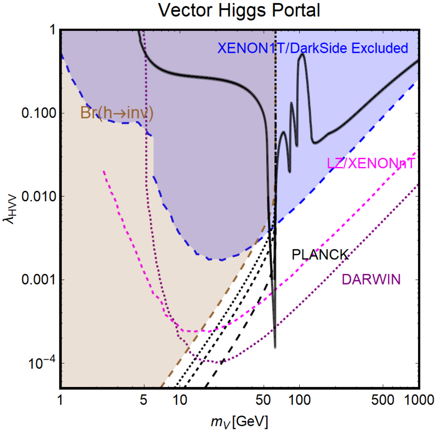
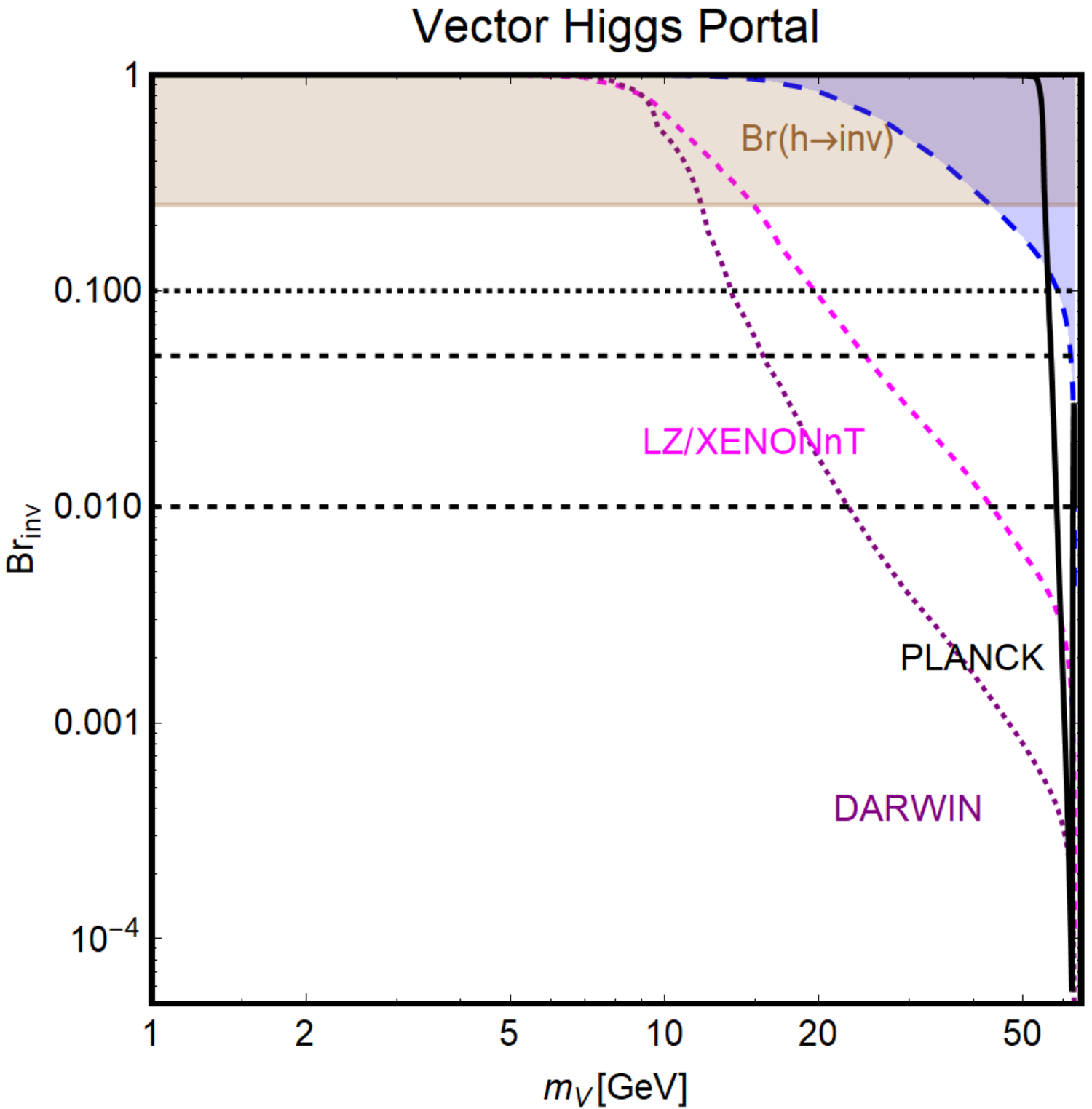
The outcome of our analysis is shown in Fig. 19. The pairs of panels in the figure correspond, respectively, to scenarios of scalar (, upper panel), fermion (, middle panel) and vector (, lower panel) DM states. Left panels show results in the bidimensional plane [, ]. The black contours, labelled as PLANCK, correspond to the correct relic density, i.e one has to lie exactly in that line to have the correct DM abundance: above the line the DM is underabundant and below overabundant. The blue regions are excluded by DM direct detection: the regions are excluded by XENON1T and, in the case of scalar and vector DM states, these exclusion bounds are complemented by a weaker constraint from the DarkSide–50 experiment [259, 260] for .
As will be discussed in more details in the next subsection, given the dependence of the direct detection rate on the local DM density, in order to draw exclusion regions like the ones shown in Fig. 19, one has to implicitly assume that the DM features the correct relic density (e.g. through a non–thermal mechanism and/or modifications of the cosmological history of the Universe [274, 275, 276, 277, 278]) even outside the “PLANCK” isocontours. The brown region is excluded by the current limit from invisible Higgs decays. The black lines correspond to BR, and . Finally, the magenta and purple lines are the sensitivity prospects of forthcoming DM direct detection experiments, LZ/XENONnT (given the similarities in the expected sensitivities, the two are represented by a unique line) and DARWIN. By sensitivity prospects, it is meant that the regions above each line will be ruled out if the corresponding experiment fails to see any signal. The same caveats mentioned for the XENON1T/DarkSide–50 excluded region apply also for these curves.
The previous outcome has been then re–cast, in the right panels of Fig. 19 in the bidimensional plane [, BR]. This type of comparisons between LHC Higgs results and astroparticle physics experiments have also been made by the LHC experimental collaborations themselves. We have, for instance, reproduced and complemented in Fig. 20 an analysis performed by ATLAS in Ref. [237].
In the figure, the main constraints for the three DM spin assignments are shown in the bidimensional plane . The dashed curves correspond to the predicted DM–nucleon scattering cross section for a DM coupling with the Higgs boson corresponding to BR, i.e. the 95%CL limit on the invisible Higgs branching ratio derived using both the visible and invisible decay channels. The dot–dashed blue/magenta/purple curves, represent, according to the previous color code, the constraints from XENON1T and the prospects from XENONnT/LZ and DARWIN. The solid lines represent the spin–independent cross section obtained by fixing the DM Higgs coupling to the correct DM relic density (the curves for scalar and vector DM overlap).

One sees that for Higgs masses below approximately 62 GeV, the LHC limits from the invisible Higgs decays, when compared to those obtained from direct detection experiments, are in general weaker and less severe as one approaches the threshold. An exception is the case of vector DM, in which the limits from LHC are competitive with the ones from direct detection in the low mass region, i.e. , where the latter are limited by the threshold in the detected recoil energies. The LHC limits for vector DM will be instead superseded by next generation of direct detection experiments.
In fact, for even smaller DM masses, –7 GeV, the sensitivity of direct detection experiments is limited by the energy threshold of the detectors (especially XENON–based ones) and the LHC plays a crucial role in constraining this possibility.
2.3.5 Uncertainties and caveats in the comparison of DM limits
As seen before, at least for DM masses above 10 GeV, direct detection experiments are much more constraining than the LHC. Nevertheless, some care should be taken when comparing the outcome of the two types of experiments. Indeed, limits from the invisible Higgs width or searches just require, to be applied, that the particle in which the Higgs decays is stable at the detector level and appears as missing transverse energy. No assumptions concerning the eventual relic density or other astrophysical properties are needed. This is absolutely not the case for direct detection limits. As a matter of fact, the DM scattering rate on a target detector depends not only on the particle physics input, represented by the DM scattering cross section, but also on the DM velocity distribution and its local density . This last quantity, in particular, serves as a normalization for the signal rate. As we have already seen, experimental limits are customarily expressed in the bidimensional plane , fixing the assignment for the astrophysical inputs according to the so–called Standard Halo Model (SHM) [160]. In this model, the DM is represented in the galactic frame, by an isotropic velocity distribution of the form
| (61) |
describing an isothermal sphere. is a normalization factor such that while is a circular velocity. The function defined in eq. (45) is the DM velocity distribution in the detector frame and satisfies the relation with and being, respectively, the Sun’s velocity with respect to the center of the Galaxy and the Earth’s velocity with respect to the Sun. The local DM density is determined from astrophysical observations either through local methods, i.e. using kinematical data from nearby population of stars, or through global methods, i.e. modelling the DM and baryon content of the Milky Way and using kinematical data from the whole Galaxy; see Refs. [279, 280, 281, 282, 283, 284, 285, 286, 287, 288] for more details.
The SHM adopts for these three parameters the fiducial values , (or 230) km/s and km/s. These parameters are nevertheless subject to sizable experimental uncertainties. For example, one has and can range from km/s to Km/s [289]. These variations in the astrophysical inputs translate into different predictions of the DM scattering rate and, consequently, weaker or stronger limits with respect to the one customarily quoted. One should also remark that the SHM provides a simplified approximate description of the DM galactic distribution, challenged by the results from the most recent DM hydrodynamical simulations, including the effects of baryons [290, 291], as well as by observational evidences from the GAIA collaboration [292, 293, 294]. Notice that a proper assessment of the astrophysical inputs is also crucial when the outcome of different experiments is compared; this problem can nevertheless be encompassed through the so–called halo independent methods [295, 296, 297, 298, 299, 300, 301].


The effect on the limits from direct detection, focussing for definiteness on the XENON1T experiment, when varying the astrophysical inputs in the signal rate is shown in two examples in Fig. 21. For simplicity we illustrate just the case of the scalar Higgs–portal. In the left panel, we follow the analysis done in Ref. [302] in which a substantial variation of the astrophysical inputs has been assumed in order to maximize the impact on the direct detection limits (this reference considered the limits from the LUX experiment but, to a good approximation, the results can be translated to the case of XENON1T since the two detectors have the same material and a similar design). In the right panel, we show, following the results presented in Ref. [291], different exclusion lines from the XENON1T experiment, obtained by replacing the DM velocity distribution of the SHM with the one inferred from the result of some recent hydrodynamical simulations. Here, we have focussed on the region where the impact of the different DM distribution is mostly prominent. In both cases, we have reported for comparison the isocontour of the correct DM relic density and the excluded region by searches of the invisible branching fraction of the Higgs boson. The impact of the astrophysical uncertainties is clear but no new viable region for the DM relic density in the effective scalar Higgs–portal is opened.
A final important remark is that normalizing the DM scattering rate with the experimental determination of (modulo the uncertainties), implies the assumption that the scattering particle represents the total DM component of the Universe and features the correct relic density. One could, in principle, relax this assumption and consider that the WIMP Dark Matter candidate represents only a fraction of the total DM component. In such a case, the DM signal rate would be normalized by a factor and the corresponding limits would be weaker than the ones presented in the previous subsection. In such a scenario, limits from searches of invisible Higgs decays can become competitive since they do not depend on .


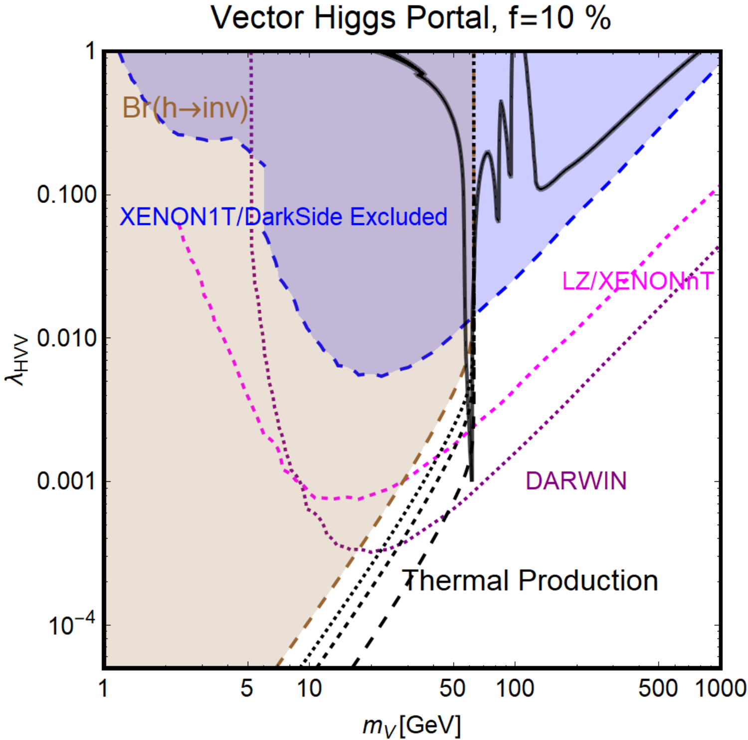
We have repeated the analysis shown in Fig. 19 in the case of . By comparison with Fig. 19 (left), one sees that the direct detection and relic density curves shifted in an analogous way towards higher value of the DM coupling. This is to be expected since the annihilation (except in the channel) and scattering cross sections are proportional to . More importantly, one notices that for , the bounds from the invisible Higgs width are comparable with the one from direct detection in the cases of scalar and fermionic DM and even more competitive in the case of vector DM. A similar reasoning as above can also be applied to the limits from DM indirect detection. But as the latter will have only a marginal impact on the results presented in this work, we will not discuss the effect of astrophysical uncertainties (for a discussion see for example Refs. [303, 304, 302]).
In the next sections, we will discuss a series of more refined and extended DM scenarios. While keeping in mind the caveats discussed in this subsection, we will nevertheless assume for the results that will be presented there, first the SHM and second that the DM candidate represents the total DM component of the Universe.
3 The SM Higgs and extended fermionic sectors
3.1 The physical landscape
As it was mentioned in the previous section, the considered effective model in which the DM particle is a singlet fermion under the SU(2) gauge group was, contrary to the vector and scalar DM cases, clearly non–renormalisable. In order to have a renormalizable interaction, at least two multiplets, whose hypercharge differ by a factor , should be present in the theory, with the DM being a mixing of their electrically neutral component (we have two require, in addition, that the DM is the lightest among the new states) [305]. In this review we will stick on the minimal option, represented by the mixing between and electroweak isodoublet and an isosinglet. Less minimal possibilities have been extensively reviewed e.g. in [306]. Appropriate options for a renormalisable Higgs–portal with a spin– DM, complying at the same time with LHC data, are the ones in which the fermions that are present belong to real representations, i.e. have Majorana mass terms, or form vector--like pairs. For instance, a simple realization are the so called singlet--doublet models99 9 More complete realizations are represented by the minimal supersymmetric Standard Model (MSSM) [41, 145] and its next-to-minimal version (NMSSM) [154] to be discussed later. [103, 104, 105, 106]. Another simple realization of a renormalizable Higgs–DM interaction is when a complete vector–like family of leptons (as well as quarks) is added to the SM fermionic spectrum [107, 77, 78, 79, 60, 108, 109]. These are the two options that we will discuss in this section, assuming that the Higgs sector is still SM–like. The fermionic Higgs–portal discussed previously can be then interpreted as an effective limit of such a setup in which the extra fermionic fields, except from the DM, are heavy and integrated out; see Ref. [157] for a concrete example.
Nevertheless, the most straightforward and obvious possible extension in this context would have been a fourth generation of fermions [98, 99, 31, 100]. The simplest version, a fourth family that behaves exactly like the first three ones, is in fact completely and unambiguously ruled out by LHC data [101, 102] but some variants have survived until recently [307, 308]. Such a scenario is worth discussing as it incorporates many ingredients that appear in other viable scenarios, and we thus start this subsection by briefly summarizing it.
3.1.1 The possibility of a fourth generation
In the extension of the SM with a fourth generation of fermions that we denote by SM4, one simply needs to add to the SM fermionic pattern with three generations, two quarks and , a charged lepton and a neutrino but with a right–handed component in such a way that it becomes massive [99]
Being a right–handed SM singlet, it is allowed to have a Majorana mass term, so that in general one can define two (Majorana) mass eigenstates and from the diagonalization of the mass matrix
| (67) |
with and being, respectively, the Dirac and Majorana masses. In the absence of a Majorana mass, the fields would form a Dirac state. As will be seen in the next subsection, a Dirac fermionic DM with non–zero hypercharge is extremely constrained as it has full couplings with the boson. We will thus conservatively stick to the case in which the fourth generation neutrino DM is a Majorana fermion. In the mass basis, the coupling of the fourth generation neutrinos to the and bosons are given by
| (68) |
where we use the abbreviations with being the mixing angle which diagonalizes the neutrino mass matrix.
In the general case in which the SM4 fermions mix with their SM light partners, two strong constraints should in principle apply on the new spectrum. First, the fourth neutrino should be much heavier than those of the three first generations, more specifically , as required by the invisible width of the boson measured at LEP1 and, in the case of the charged lepton, the LEP2 bound GeV should apply [36]. Second, direct LHC searches exclude too light fourth generation quarks with masses close to the unitarity bound, GeV [309, 310, 311]. However, if mixing between SM4 and SM fermions is forbidden by some symmetry and if one assumes that the DM neutrino interacts only with the Higgs boson, some of these constraints can be evaded (see later for a summary of these constraints).
Nevertheless, if the new fermions acquire masses through electroweak symmetry breaking as in the SM, strong constraints can also be set on the SM4 scenario from the measurements of the Higgs properties at the LHC. This is due to the fact that in the loop induced and couplings, see Appendix A1, any heavy particle coupling to the Higgs proportionally to its mass, as it should be also the case in SM4, will not decouple from the amplitudes and have a drastic impact. In particular, for the dominant production process, the additional and contributions increase the rate by an order of magnitude at leading order (LO). However, large electroweak corrections affect these couplings [312, 313, 314, 100] resulting, in the usual SM4, in a very strong suppression of the rate to the level where the channel becomes unobservable at the LHC.
To illustrate this feature, using a version of HDECAY for SM4 which includes these next–to–leading order (NLO) corrections, the rate for GeV is shown as a function of the masses and GeV in the left–hand panel of Fig. 23. One notices that it is a factor of 5 to 10 smaller than in the SM despite of the increase of by a factor of in SM4. In the right–hand side of the figure, the ratio in SM4 shows that the signal rate would be reduced by a factor 3 to 5 depending on . Looking at the Higgs signal strengths discussed in the previous section and shown in Fig. 2, it is clear that the possibility of a fourth fermion family is excluded in such a case.
Nevertheless, in Higgs–portal to DM models, some protecting symmetry like a parity should be present to forbid or suppress the transitions between the SM4 fermions and the ones of the first three generations. This will allow the lightest of them, the fourth neutrino, to be stable and, as it should also be massive, to be a good candidate for DM. In this case, the decay pattern of the charged heavy fermions becomes rather complicated as will be discussed in the next subsection, invalidating the usual experimental bounds on new quarks and leptons decaying into light SM ones and gauge or Higgs bosons. In Refs. [307, 308], it was advocated that within such a scenario, quark masses as small as a hundred GeV are possible and could modify significantly the phenomenology of the SM4 model.
Indeed, in the case where GeV, the suppression of the decay width, as a result of the negative interference between the boson and the heavy quark loops, will not be drastic and a rate would be possible. This has to be contrasted with the previous case in which the quarks had to be as heavy as 500 GeV and a two order of magnitude suppression of the rate took place. As the contribution of the extra quarks in gluon fusion lead to a cross section ratio , one could ultimately arrange so that is very close to the SM value measured at the LHC. However, in order to fix the rates for the other detection channels, in particular and , the increase of the production cross section should be compensated by a suppression of the and branching ratios which result from the additional Higgs decays into the invisible SM4 neutrino, . One can then choose the values of and which enter in the expression of this decay width (both directly and in the phase space) in such a way that it suppresses by an order of magnitude the branching fraction of all visible Higgs decays.
Following the analysis presented in Ref. [307], we have delineated the region of the plane in which this occurs, namely the region enclosed between the two green lines in Fig. 24. In this area, the signal strengths for all Higgs decay channels measured in the dominant gluon fusion mechanism, in particular but also if the masses of the new quarks are also chosen appropriately, are compatible with the LHC measurements shown in Fig. 2 [307, 308]. The depicted scenario is nevertheless very problematic as also shown in Fig. 24. First, in order to obtain the correct fit of the signal strengths into gauge bosons, the SM Higgs boson should decay invisibly, i.e. into pairs of fourth generation neutrinos, to a large extent. Indeed, the brown area depicted in Fig. 24 leads to an invisible Higgs branching that is larger than 20%, the value excluded by LHC measurements and searches, and includes the area compatible with the signal strengths.
In addition, the sizable couplings between of the DM with the Higgs and bosons imply too strong annihilation processes for the DM state, so that it can contribute at most to a fraction of the total DM component unless some non–thermal production mechanism is assumed. For the same reason, very large scattering cross sections of the DM on nuclei are expected. As shown by the blue region in Fig. 24, even if one considers rescaling the direct detection exclusion limits with a factor as discussed in the previous section, sizable regions of the parameter space are ruled out.

One should finally note that there are other Higgs production channels besides gluon fusion and some of them, such as VBF and HV, have been also probed by the LHC experiments. In the scenario above, the Higgs decay signal strengths measured in these two production channels would have been an order of magnitude lower than in the SM and thus, in total contradiction with the values shown in Fig. 2 which are compatible with the SM at the level of a few 10%. This can be, in fact, seen from the recent observation of the Higgs boson in the channel which mainly proceeds via the process which is not affected by any loop, except for those appearing in the NLO radiative corrections which tend to suppress the rate, see Fig. 23 (right), while is affected by the same ingredients as the other visible decays probed in gluon fusion. The signal strengths measured by the ATLAS and CMS collaborations, [209] and [210], leave no chance for this scenario to occur.
Hence, even in the less constrained case in which the SM4 fermions do not mix with the standard ones leading to a stable DM heavy neutrino, the possibility of a fourth generation and, more generally, of new fermions whose masses entirely originate from the Higgs sector of the SM, is totally excluded by the LHC Higgs data.
3.1.2 Singlet–doublet DM model
A most economical extension of the fermionic DM sector to accommodate renormalizable interactions with the Higgs field is the so called singlet–doublet model (SDM) [103, 104, 105] which, as mentioned earlier, has the additional advantage of representing a simple limiting case of well studied scenarios such as the MSSM [41, 145] and its extensions such as the NMSSM [154], hence providing a very useful benchmark for supersymmetric scenarios1010 10 Notice, however, that in these two SUSY cases the DM state can have, besides a singlet (bino and/or singlino) and a doublet (higgsino) component, an SU(2) triplet (wino) component.. In this model, two additional doublet and a singlet fermionic fields are introduced
| (69) |
which lead to different quantum assignments compared to those of the SM leptons (instead, one should note that the and fields have the same quantum numbers as the higgsinos and of the MSSM as will be seen later). Their masses and interactions with the SM Higgs field and its conjugate field are defined by the following Lagrangian
| (70) |
The three lepton states are described by the following mass matrix
| (71) |
which can be diagonalised with a unitary matrix , leading to three Majorana mass eigenstates1111 11 A realization of the singlet–doubled model with a Majorana DM has been proposed in Ref. [106]. It will not be reviewed here since its phenomenology features strong similarities with the one of the model proposed in the next subsection.
| (72) |
the lightest of which, , is assumed to be the DM candidate. The mass spectrum of the new states is completed with an electrically charged Dirac lepton with a mass . Note that the Lagrangian of eq. (70) is defined under the assumption that the new fermions are odd under a symmetry, with the SM states being even, so that couplings through the Higgs boson between new and SM fermions are forbidden. Furthermore, given the transformation properties of the fields , under the discrete symmetry, only one between the signs of the mass term and of the couplings and is physical. We will assume here a positive sign for and leave free the signs of and .
In the physical basis, the interaction Lagrangian of the new fermions reads
| (73) |
with and as defined earlier. The vector and axial–vector couplings of the fields to the boson are given by
| (74) |
showing that, as expected for Majorana fermions, the coupling of the DM with the boson is only axial–vector like. The couplings between the neutral states , their charged partner and the bosons are instead given by
| (75) |
The last term of the Lagrangian eq. (3.1.2) represents the coupling between a DM pair and the Higgs boson, already introduced in the simple Higgs–portal model previously discussed. The couplings with the Higgs boson are explicitly given by
| (76) |
In our study, we will trade the parameters with the parameters so that [105]
| (77) |
Note however, the presence of the hypercharge and SU(2) components for the DM particle, inherited from the mass mixing between the vector–like lepton, which implies couplings also with the and bosons, in contrast to the effective Higgs–portal model. This feature has a very strong impact on the phenomenology, as will be shown later.
As already mentioned, the Majorana singlet–doublet model can be interpreted as a simplified version of a supersymmetric scenario. By performing the following substitutions
| (78) |
it is straightforward to identify the SM singlet state with the bino (or alternatively the singlino in the NMSSM) with the Majorana mass parameter , and the , as already said, with the higgsinos, with a mass parameter . The angle is defined, as usual, such that represents the ratio of the vacuum expectations values of the two Higgs doublets in the MSSM/NMSSM. The singlet–doublet model can be then seen as a supersymmetric model with mixed bino/higgsino DM in which all the scalar states, apart from the SM–like Higgs boson are integrated out; see section 6.
3.1.3 Extensions with vector–like fermions
The fermionic spectrum can be extended in a theoretically consistent and renormalisable way, while evading the stringent bounds from the 125 GeV Higgs data and direct searches that apply in the fourth fermionic generation case, also with families of vector–like fermions (VLF). While less-economical with respect to the case of the singlet-doublet model discussed in the previous subsection, it is of great phenomenological interest since allows, as clarified below, for modification of the Higgs signals at colliders. We define a “family” of VLFs as a set of states composed by two singlets and one doublet, all of them belonging to a same representation of SU(3) and with a hypercharge which can be expressed in terms of a unique parameter as follows
| (79) |
In this setup, a VLF family can be described, in terms of the SM Higgs field and the decomposition for the SU(2) doublets , by the Lagrangian [109]
| (80) |
According to the color and hypercharge assignments, the VLFs can share the same quantum numbers as SM quarks and leptons; in this last case, however, neutral singlets analogous to right–handed neutrinos would be present as well. This would imply the presence of mixing between the vector–like and the SM fermions with the same quantum numbers. This mixing would allow for the decays of the VLF fermions, including an eventual DM candidate, into SM states, originating a tension with requirement of stability at cosmological scales for the DM. We will thus impose the discrete symmetry, dubbed , under which the VLF and the SM fermions feature opposite charges, so that their couplings with the Higgs boson and the subsequent mixing, will not allow for this possibility.
The states that appear in eq. (79) are in the “interaction” basis and, after electroweak symmetry breaking, their coupling with the Higgs boson induces a mass mixing between the “up” () and “down” () states, having the same electric charges, and respectively, described by the following transformation:
| (81) |
where the sub/superscripts distinguish between the two sectors. Here, we will denote the lighter mass eigenstate as . The limit where one of the singlets is decoupled, e.g. when and , has been studied in detail in Ref. [315]. The mass matrices for the “up” and “down” states are defined as
| (82) |
In our analysis, we will consider the assignments for the hypercharge and the color index of the vector–like lepton families. In this case, the new fermions have the same quantum numbers as a generation of SM leptons plus additional right–handed neutrinos. This is why we will call them “VLLs” and we adopt for them the notation
| (83) |
The vector–like lepton family features electrically neutral states, the neutral components of the doublet as well as the “right–handed” vector–like neutrinos, the latter being complete SM singlets. It is then evident that the DM particle can be potentially embedded in this kind of construction. In this review we will consider the case that the mass eigenstate corresponding to the DM candidate is a Dirac fermion. Majorana DM can be nevertheless accommodated in this setup as shown, e.g., in [316].
For many reasons, such as chiral anomaly cancellation, VLLs should always be accompanied by vector–like quarks (VLQs) in order to form a complete family. In our analysis, we will sometimes consider such a family of VLFs with the leptonic sector chosen as above and for the quark sector, we assume that the new quarks have the same quantum numbers as a generation of SM quarks with and , using the following notation
| (84) |
We now illustrate in more detail the features of the family of vector–like leptons related to the DM heavy neutral lepton. For a single vector–like family, the Lagrangian with the particle content of eq. (79) reads
| (85) |
After the breaking of the electroweak symmetry, the spectrum of the new fermions features two neutral states with masses and two electrically charged states with masses obtained by rotating the mass matrices
| (86) |
with pairs of unitary matrices , of angles
| (87) |
The two mixing angles are given by
| (88) |
while are obtained by replacing and in the expressions above. In this scenario, the DM candidate is the state if it is lighter than the charged fermions . In the mass basis, the DM interaction Lagrangian can be written as
| (89) | |||||
where the couplings, using the abbreviations etc…, are
The couplings are obtained from by the exchange in the labels.
3.1.4 Theoretical constraints
To have a theoretically consistent picture, the couplings of the new fermions in extensions of the SM should obey severe requirements. First, these fermions affect the running of the SM gauge couplings, potentially leading to Landau poles at low energies. The Yukawa couplings of these states are also subject to evolution with energy and could enter a non–perturbative regime if they are set to too high values at the electroweak scale. More important, the new Yukawa couplings also affect the renormalisation group evolution of the Higgs quartic coupling, possibly rendering it negative and hence destabilizing the potential in a way such that electroweak symmetry breaking does not occur.
We illustrate in this subsection, the impact of these renormalisation group constraints taking the case of vector–like fermions as an example; we will restrict to the leading order, which makes that our discussion can be viewed to be only qualitative since it is essentially based on these one–loop ingredients.
The one–loop functions for the gauge couplings with and in the presence of and vector–like leptons and quarks can be written as
| (96) |
From these equations, one can see that the functions get positive contributions that depend on the multiplicity of the VLF families and, in the case of the U(1) coupling , on the hypercharge of the new states. Too large positive contributions would lead to Landau poles, i.e. , at some scale . In this work, we will thus consider, also for the sake of minimality, the case of only one vector lepton family with and without a vector–like family, or 1.
The evolution of these couplings is shown in Fig. 25 as a function of the energy scale and, as one can see, the running is not affected to a pathological extent by the presence of a sequential family of vector–like leptons or even by a full family of vector–like fermions, so that the gauge couplings remain perturbative up to .

For the self–coupling and the Yukawa couplings , the situation is quite different. Their functions are given by
| (97) |
where we have used the abbreviations,
| (98) |
As can be seen, the function of the Yukawa couplings of the new fermions are proportional to the couplings themselves to the third power, and they vary significantly with the energy scale in contrast to the gauge couplings. Consequently, the Yukawa couplings of the new fermions can become non–perturbative at relatively low energy scales, if they are at the weak scale. More important, this potentially strong variation with energy would dramatically affect the running of the quartic Higgs coupling , since its function would receive two negative contributions proportional to and . A too steep increase of the Yukawa couplings would then drive the quartic coupling to negative values, destabilizing the scalar potential.
As was discussed in Refs. [316, 109] e.g., it is possible to obtain constraints on the size of the Yukawa couplings by solving the RGEs for the quartic Higgs coupling in combination with the ones of the new fermions, the top Yukawa and the SM gauge couplings.


We illustrate through an example, the results of such an analysis in Fig. 26. For simplicity we have considered the case . The left panel of the figure shows the value of the self-coupling as a function of the energy scale , in the case where the SM is augmented by a full family of vector–like fermions which, for simplicity, have been assumed to have the same mass GeV. The lepton Yukawa couplings have been set to , while keeping and ; these new Yukawa couplings have been assumed to be zero below the scale . As is clear from the figure, too high initial values of the coupling , namely in the specific case considered here, would make that the Higgs quartic coupling becomes negative immediately after the energy threshold , hence destabilizing the scalar potential.
A slightly more refined analysis, which gives an idea of the size of the Yukawa couplings as well as the energy scale for which the scalar Higgs potential becomes instable, is summarized in the right–hand side of Fig. 26. Shown as a function of the coupling and for the same values of the model parameters considered in the left panel of the figure, the stability scale . The latter corresponds to the scale at which the negative runaway of the effective potential takes place which, following an analysis performed in Ref. [317], can be defined by the condition which roughly indicates the onset of vacuum instability. As can be seen from the figure, values are needed in order that the instability scale lies significantly above the TeV scale.
Before closing this subsection, let us again emphasize the fact that one should not interpret the results from these renormalisation group analyses as strict constraints on the model parameters, but simply as an indication that the theory requires a further ultraviolet completion, through the introduction of suitable additional degrees of freedom at the scale . It is sufficient to ensure that the scale is sufficiently above the energy scales relevant for collider and astroparticle phenomenology, which will be discussed later.
3.2 Constraints on the new leptons and expectations at colliders
We now turn to the phenomenology of the new leptons (and their possible partner quarks) that accompany the DM particle in these models and summarize the various experimental constraints to which they are subject. The production of the new states at colliders is described at the end of the section. For additional discussions, eventually outside of the DM context, see for instance Refs. [318, 319, 133, 320, 321, 322, 323, 324, 325, 326, 327, 328].
3.2.1 Constraints on masses and couplings
Let us start by describing the couplings of these particles to the SM ones in a slightly more general form that suits at the same time the two cases that are under discussion here, namely singlet–doublet and vector–like leptons. Except for the singlet DM particle which should have no electromagnetic nor weak charges, the other singlet–doublet like or vector–like fermions couple to, besides the Higgs boson, the photon when electrically charged and the electroweak gauge bosons with typical electroweak strength. These couplings allow for the pair production processes of these particles at colliders. For a generic lepton which could be either or with being the lighter DM state (from now on, we omit the subscripts for simplicity) with electric charge or in units of the proton charge and left– and right–handed isospin assignments and , the vector and axial–vector couplings to gauge bosons are given by eqs. (19) and (20) in the and cases, respectively. Hence, in the vector–like case, the axial–vector couplings to the boson are zero by construction; in addition, the fermion couplings to the boson are twice as large as the ones of SM fermions.
Because of the symmetry under which the new fermions are odd while the SM ones are even, there should be no mixing between the two types of fermions. The heavier states should then decay into lighter companions and gauge or Higgs bosons, bosons for charged decays and bosons for neutral decays. At the end of the chain, there must be the lightest odd particle which is our DM candidate, namely one of the additional neutrinos. In this case, the signatures will consist into missing energy and Higgs or gauge bosons, the so–called mono–Higgs or mono– signatures. If the mass splitting between the parent and daughter new particles in the decay is small (as is required by the electroweak precision data to be discussed later), the intermediate bosons will be off mass shell and will decay into a pair of almost massless fermions, or for example (because the couplings to light fermions is very small, the intermediate states are in general the weak bosons). The smaller is the mass difference between the heavier new leptons and the DM particle, the softer are the final state fermions so that the signatures will be rather difficult to detect, in particular at hadron colliders.
In the case of the heavy quarks that appear when one considers a full vector–like fermion family, some amount of fermion mixing should be possible in particular if baryon number is conserved. This will allow the new quarks, or at least the lighter one since here also there might be decays of heavy to lighter new quarks , to decay into the SM ones and some gauge or Higgs bosons, . However, the mixing angle should be very small and the lifetime of the new fermions could be very long making that they decay outside the detectors of collider experiments which, in practice, make them almost stable in this context and hence not straightforward to detect.
The present experimental constraints on the masses of the new heavy leptons and quarks depends on whether they are considered as stable or not and we summarize those quoted by the Particle Data Group [36] in the following. In the case of a Dirac DM neutrino which should be stable, a limit of GeV has been set from the accurately measured invisible decay of the boson at LEP1; if the neutrino is of Majorana type1212 12 In the case of Majoranas, the couplings to the boson are only axial–vector like and the partial widths are suppressed by three powers of the velocity compared to only one power in the Dirac case where the couplings are vector–like; the partial width is thus much more suppressed near the phase–space boundary, . the limit is slightly weaker, GeV. In the case of the charged leptons, there are bounds from searches at LEP2 with a c.m. energy beyond GeV [329, 36]: GeV for a stable lepton and GeV if it decays into a light neutrino and a boson. For heavy neutral leptons that are not stable, bounds from LEP2 searches also apply and give GeV for a Dirac and GeV for a Majorana state [329, 36].
In the case of quasi-stable quarks, the only bound that is quoted is the one on a –like quark, GeV from searches at the Tevatron, besides the one from decays at LEP1, GeV [36]. If the heavy quarks decay visibly into light SM quarks and gauge or Higgs bosons, bounds from negative searches at the LHC are much more severe. This is particularly true for the heavy partners of the top and bottom quarks for which bounds of about TeV are set on their masses at LHC with TeV depending on the isospin and branching fractions, and above GeV in essentially all cases [36].
Coming back to the new leptons and the searches that have been performed at the LHC, the charged ones under the electroweak group can be pair produced in proton collisions through the Drell–Yan processes of the type (details will be given later on) [330]
| (99) |
with the charged fermions subsequently decaying into a (either on– or off–shell) and a neutral lepton (typically the lightest one, i.e. the DM candidate) while the heavy neutral fermions feature different possible decay channels, i.e. into a lighter one and a (again either on– or off–shell) or possibly boson or the charged fermion and a boson. The relative strength of the possible signals depends on the amount of hypercharge and doublet components of the new lepton fields, set by the elements of the mixing matrix or by the angles in the two cases that we are interested in. The cleanest signature is in general represented by events with missing energy accompanied by multileptons.
A detailed classification of all the possible event topologies has been presented for instance in Ref. [105] in the case of the singlet–doublet model and we refer to it for details. In this case, among all these processes, the strongest constraints come from the charged current channel which leads to a three leptons plus missing energy signature. The limits obtained by CMS and ATLAS in various searches that mimic this topology, see for instance Refs. [331, 332] for the most recent ones, should be appropriately recast in order to be applied for the scenario under consideration. Such recasting has been performed, for example, in Ref. [333] for analyses of the set of data [334, 335]. It has been found that these searches constrain the regions for the heavier short lived leptons and for the stable DM lepton. One should however note that these constraints mostly apply to the case and in the opposite case, the lightest neutral leptons are mostly doublet–like and are very close in mass with the charged state . This type of configuration is more complicated to probe at hadron colliders since it would correspond to the production of long–lived particles, leading to displaced vertices or particles being eventually stable at the detector level.
3.2.2 Constraints from electroweak observables
Besides these direct collider constraints, there are also indirect ones as these new fermions interact with the gauge bosons and thus affect electroweak precision observables (EWPO) [336, 115, 337, 338, 316]. Depending on their masses and their gauge and Yukawa couplings, they could induce large deviations with respect to the SM predictions. It turns out that, to a good approximation, the contributions induced by the new fermions can be mapped into corrections to the parameter [339] which historically was used to measure the strengths of the ratio of the neutral to the charged currents at zero–momentum transfer, . In the SM, this parameter is equal to unity at tree–level as a result of an SU(2) custodial symmetry but it receives higher–order corrections, via the and boson self–energies , parameterized by
| (100) |
The contribution of two particles with masses to the boson self-energies and hence to the parameter (factorizing out complicated coefficients of the couplings to gauge bosons and ignoring higher orders for simplicity) read
| (101) |
The function vanishes if the and particles are degenerate in mass while, in the limit of a large mass splitting, one has instead.
Hence, in the case where the members of an SU(2) doublet have masses that are quite different, contributions that are quadratic in the mass of the heaviest particle appear. As the parameter has been measured with a precision of a fraction of a permile and found to agree with the SM expectation [36], it sets a very strong constraint on the mass splitting between the two leptons that belong to the same SU(2) isodoublets.
More precisely, the new states will not only contribute to the parameter above but more generally to the Peskin–Takeushi parameters [340]. While the leading New Physics contributions i.e. is denoted by , namely , parametrizes the New Physics contributions to neutral current processes at different energy scales while the parameter describes new charged current contributions to the boson mass. A global fit to all electroweak precision observables available today has been made leading to the following [341, 342]
| (102) |
determined as functions of the deviation of the parameters with respect to their SM corresponding values
| (103) |
with the standard deviations and the covariance matrix given by
| (104) |
We have calculated these radiative corrections adapting the complete and general expressions quoted in Ref. [316] to our two singlet–doublet and vector–like lepton cases.

The regions excluded by precision observables in the singlet–doublet scenario are shown in Fig. 27 in the plane for the value and three assignments for . As discussed in Refs. [343, 105], these bounds are not very effective in this scenario as they essentially affect only the parameter. As can be seen from Fig. 27, only a portion of parameter space at small values of is excluded. This is because, in this region, , implying sizable mass splitting between the SU(2) doublet states. The different extension of the excluded regions with is explained by the fact that the contribution of the new fermions to the parameter is proportional to . Consequently, the excluded regions grow with while, in turn, we have for . As will be justified later, we have focused in Fig. 27 on the case where as it is more interesting for DM phenomenology in the astroparticle physics context.


The case of a full vector family is more complicated as a result of the larger number of free parameters, i.e. three masses, , and four Yukawa couplings and . In this scenario, both the and parameters receive substantial contributions that can be fully described only if an extensive numerical analysis based on eq. (102) is performed. In the left–hand side of Fig. 28, we nevertheless show two examples of the constraints that can be set on the plane for , and two assignments of the couple , namely and .
We have marked in red or orange the regions of the parameter space that lead to values of the precision observables that are less than three standard deviations from the experimental measurements and, in order to facilitate the understanding of the figure, we have also drawn isocontours of the deviations and from the SM expectation. As it can be seen, the allowed regions are mostly determined by the constraint on the parameter which can be evaded only by imposing, at least partially, a custodial symmetry,
| (105) |
This requirement is particularly severe at high values of the Yukawa couplings, . This is exemplified in the right–hand side of Fig. 28, where we show the same electroweak constraints but in the plane again for GeV and fixing the other lepton masses to GeV. Large Yukawa couplings close to unity are allowed only if . Notice that in our analysis, we have from the start assumed . Besides reducing the number of free parameters, this choice ensures to comply with collider bounds on the Higgs signal strengths, as will be clarified below.
3.2.3 Constraints from the Higgs sector
New fermions coupled with the Higgs boson and, at least partially, charged under the SM gauge group, can generate possibly large modifications of the Higgs couplings to SM fermions and gauge bosons which are tightly constrained by the measurement of the Higgs signal strengths at the LHC. Among the two SM extensions considered above, only the one with a full family of vector like fermions is phenomenologically relevant in this regard. In this last case, given the absence of mixing between the SM and the new fermions, only the couplings of the Higgs with the SM gauge bosons are affected. If the SM is extended by only vector–like leptons, the effective coupling of the Higgs boson with two photons is affected in the most significant way. In the case where vector–like quarks are also present, modifications of the effective coupling with gluons are relevant as well. We will thus focus our discussion on these two couplings.
In presence of new leptons, the decay amplitude of the Higgs into diphotons is given by
| (106) |
where are the SM and New Physics contributions, respectively. The latter can be schematically written as
| (107) |
where is the loop function for spin– particles given in Appendix A1, for which we have take for simplicity the asymptotic limit , which is a good approximation for GeV as it should be the case here. Notice that the sign of relative to is not fixed but determined by the sign of the function defined as
| (108) |
In absence of modification of the effective Higgs coupling to gluons, the Higgs signal strength can be written in this case as
| (109) |
As it should be clear from eq. (107), the New Physics contribution to the Higgs decay amplitude into diphotons is proportional to the product and, consequently, vanishes if one of these couplings is zero. The contribution also decreases with the masses of the charged vector leptons. In order to asses the impact of the contribution of the new sector to the diphoton Higgs signal strength , we have performed a scan of the parameters over the following ranges
| (110) |
The result have been confronted to the experimental determination and shown in the left panel of Fig. 29 as a function of . One can see that deviates with respect to the measured value mostly for masses of the lightest charged vector lepton below 200 GeV. New Physics effects tend instead to rapidly decouple at higher masses.


We have then focussed on the range and we show in the right panel of Fig. 29 the points of the plane which lead to a value compatible with the LHC constraint. One sees that most of the viable model points can have up to 3, provided that the other Yukawa coupling is very small, below . Nevertheless, there is a limited set of solutions with even higher values of the Yukawa couplings: it is indeed possible to have a viable for high Yukawa couplings in the case in which a cancellation occurs between the SM and new contributions to the Higgs diphoton rate, such that . By using eq. (107) and assuming for simplicity and , the latter requirement can be translated into the following simple equation [108]
| (111) |
3.2.4 Prospects for heavy leptons at colliders
We now discuss the prospects for producing the new leptons at high-energy colliders (some elements have been touched upon in the previous section). First, because they couple to gauge bosons with full strength, heavy non–singlet leptons can be pair produced in proton–proton collisions [320, 321, 322, 323, 324, 325] in the Drell–Yan process , eq. (99). The cross section will only depend on the electric charge and weak isospin. In the case of an electrically–charged state, both the and boson channels and their interference have to be included, while only the channel with boson exchange has to be considered for a neutral lepton (which stands now generically for all heavy neutral leptons) with electroweak couplings. The cross sections for pairs of charged or neutral leptons with velocities at partonic c.m. energy simply read
| (112) |
where the electron and heavy lepton couplings are given in eq. (19). In addition, one could produce pairs of charged and neutral leptons via boson exchange, . For comparable masses, , the partonic cross section is given by
| (113) |
The cross sections for producing pairs of charged and neutral vector leptons with masses GeV are shown in Fig. 30 at a proton collider as a function of the total energy [133]. The heavy leptons considered have the assignments for electric charge and weak isospin and . One notices that the rates are much smaller for the neutral processes with exchanges than for the charged one with exchange: the cross sections for production are comparable and are only at the fb level at RunI LHC while they are a factor 20 larger for production. The latter process is thus the best probe of heavy leptons in pair production. Note also that the rates increase by two orders of magnitude when moving from a TeV to a TeV collider.
In the case of an entire vector–like family, some quarks should also accompany these leptons and their production at hadron colliders is more favorable. Indeed, as they couple to gluons like SM quarks, they can be pair produced in the strong interaction process with rates that depend only on the mass and the strong coupling constant (single production with a SM quark is suppressed by the tiny or null mixing angle) [318, 319, 133]. The total hadronic cross section, i.e., after folding with the parton luminosities (which are taken here to be those of the MSTW2008 fit [208]), is shown in Fig. 31 as a function of the heavy quark mass for several center of mass energies [133]. For TeV, the cross section is at the few fb level at TeV and increases by more than one order of magnitude at or 14 TeV and four orders of magnitude at TeV. For higher quark masses, the increase of the rate with energy is even steeper, highlighting the advantage of a higher energy proton collider in this context.
Before closing this section, we should briefly comment on the production of the heavy leptons at future high–energy colliders. There is first lepton pair production just like in the Drell–Yan process at hadron colliders, , which is kinematically possible for masses . As in pp collisions, the total pair production cross section is given in terms of the usual couplings to the photon and boson by [326, 327, 328]
| (114) |
The cross sections for pair producing that are part of the same isodoublet are shown in Fig. 32 as functions of the energy for the masses GeV. Again, the rate is much smaller for the neutral compared to the charged leptons, as the process proceeds only through boson exchange for the former but the rates are still large, above 10 fb in the chosen example, to easily detect the particles in the clean environment. Of course, the production rates are higher for lighter leptons, i.e with masses that are closer to the present limit of GeV.
Another process of interest in collisions is associated production of the lepton pair with the SM Higgs boson, . This process is similar to associated Higgs production with top quark pairs, [344, 345], which has been discussed in the context of the SM. Compared to the latter, the cross sections should be smaller as a result of the absence of the color factor and the presumably smaller Yukawa couplings but this might be partly compensated by a more favorable phase space, since one can consider the associated production with the lightest neutral fermion, i.e. the DM particle, which has a mass as low as GeV from present constraints. The signature in this case would be a mono–Higgs topology since the neutral heavy leptons are invisible. The charged leptons which are expected to be heavier, might have larger rates as a result of the additional photon exchange contribution and would lead to events with Higgs bosons, light SM fermions from the decays into on– or off–shell bosons and missing energy.
Also in Fig. 32, we have displayed the cross sections for the process with the leptons being with masses GeV and with Yukawa couplings that are similar to the SM–like ones, . For this set of parameters, the rates are still significant, being only one order of magnitude smaller than those for lepton pair production and follow exactly the same trend with phase–space. For couplings compatible with LHC Higgs data, the rates should be much smaller though.
Finally, concerning the eventual heavy quark partners that would appear when a full vector–like fermion family is considered, one would need a very high energy collider such as the CLIC machine in view of the bounds on the masses of these particles (in particular if they decay inside the detectors into light quarks and gauge or Higgs bosons). Even in that case, the cross sections are not that large as the production occurs through –channel boson exchange which, as in the case of leptons eq. (114), are suppressed like at high center of mass energies. The best place for these hadronic states is thus definitely at proton machines as shown before.
3.3 Constraints from astroparticle physics
3.3.1 Constraints in the singlet–doublet model
For what concerns the DM phenomenology from the astroparticle physics perspective, the singlet–doublet scenario presents sizeable differences with respect to the effective fermionic portal discussed in the previous section, a feature primarily due to the DM couplings with the gauge bosons which are absent in the latter scenario. As the DM state is a Majorana fermion, no new spin–independent interactions are present since they require a vectorial coupling between the DM and the boson which is automatically zero in the Majorana case [346]. As a consequence, the spin–independent scattering cross section of the DM on protons is again given by an expression of the type
| (115) |
where the Higgs to DM coupling, eq. (76), is explicitly given by
| (116) |
and, as can be seen, it has a rather complicated structure and depends on many different parameters. In particular, it becomes zero in the case where the condition is met. Spin–independent interactions would then encounter a so–called “blind spot” [347, 348] since there will be no Higgs exchange channel there.
Contrary to the case of the effective Higgs–portal model, spin–dependent interactions are present in the singlet–doublet model as a result of the axial coupling of the DM with the boson. The corresponding cross section is given by
| (117) |
and it can also vanish if the coupling which, as can be seen from eq. (75), occurs for the configuration .


Concerning the relic density, the main DM annihilation channels are again into SM fermions pairs as well as final states, induced by –channel Higgs exchange but also exchange. Moreover, annihilation processes into gauge boson final states can be mediated by –channel exchange of the new fermions. Approximate expressions for the corresponding cross sections are given in Appendix B.3.1.
In contrast to the effective Higgs–portal model, the annihilation cross section into pairs of SM states features an –wave contribution. The latter is nevertheless helicity suppressed, being proportional to the mass square of the final state fermion, implying that the cross section is dominated by its –wave term. On the contrary, the additional –channel diagrams are responsible for unsuppressed –wave contributions to the and annihilation cross sections. The coupling of the DM with the boson gives finally rise to the additional final state , with respect to the effective Higgs–portal model of the previous section. Given the presence of –wave dominated cross sections, the singlet–doublet model is potentially testable also through indirect detection. The corresponding limits are, however, not competitive with the ones coming from direct detection and, hence, will not be explicitly reported here. For more details, see eventually Refs. [105, 34].
Given the small number of free parameters in the model, a nice illustration of the DM phenomenology can be achieved by varying the two masses while keeping fixed the parameters and . The outcome of such an analysis is shown in Figs. 33 and 34.
In Fig. 33, we have considered an “MSSM–like” assignment of the coupling, i.e. , accompanied by four choices of , and . For these couplings, the correct relic density, indicated by the black isocontours in the figure, is achieved in proximity of the diagonal , representing the so called “well tempered” DM regime [349, 350], until it becomes saturated for by a mostly doublet–like DM. Notice that in our analysis, we have neglected the Sommerfeld enhancement [351, 352, 353, 306] which would be responsible for a slight shift of the saturation of the mass value to . Since, contrary to the MSSM, is a free parameter, we have repeated in Fig. 34 the same analysis but taking , to highlight the possibility of achieving the correct relic density for a mostly singlet–like DM state.
All the benchmarks presented are, nevertheless, strongly affected by the bounds from DM direct detection. The only surviving regions appear to be those related to the mostly doublet regime at and some some limited regions of the parameter space (see e.g. the top right panel of Fig. 34) where direct detection constraints are weaker thanks to the occurrence of the blind spots which for our sign convention arise only for negative . The singlet–doublet model will be ruled out for DM masses up to a few TeV in the absence of signals at the next direct detection experiments.


In the analysis shown in Figs. 33 and 34, we have focused on the region , where the considered scenario is expected to feature the largest differences with respect to the effective Higgs–portal and in order to comply with the bounds from LEP on the mass of the new charged fermion. A focus on lighter DM has been instead made in Fig. 35. The two benchmark considered in the figure are characterized by two high negative values of , namely and , for which the blind spot in direct detection is achieved for a high value of , corresponding to a mostly singlet–like DM state (we recall that a mostly SU(2) doublet DM would be depleted too efficiently in the early Universe [351]).
As it is clear from the figure, in the low mass regime the relic density isocontours show two “cusps”, corresponding to –channel resonances for and . This result is in contrast with the effective Higgs–portal where only the “pole” at is present. Despite the presence of sizable portions of parameter space in which the DM spin–independent cross section is suppressed by the occurrence of blind-spots, the considered benchmarks are still in strong tension with DM direct detection as a result of the complementary constraint (green region in the plot) from spin–dependent interactions, as given by the LUX collaboration [354] 1313 13 In the final stage of the work, the XENON1T collaboration released slightly stronger exclusion bounds on spin–dependent interactions [355].. Fig. 35 shows also the impact of the constraints from the invisible decay widths of the and Higgs bosons which, similarly to the case of the effective Higgs–portal discussed previously, appear to be in general less competitive than the bounds from DM direct detection.
3.3.2 Constraints on the vector–like lepton DM
We now turn to the case of vector–like leptons. The DM being a Dirac fermion, some differences with respect to the singlet–doublet model emerge. Concerning the relic density, the most relevant annihilation channel is now represented by the one into , the corresponding cross section being not anymore helicity suppressed, thanks to the presence of a vectorial coupling between the DM and the boson. The expressions for the annihilation cross sections are given in Appendix B.3.2.
The Dirac nature of the DM has an even more significant impact on DM direct detection since the vectorial coupling of the DM with the boson is responsible of the dominant contribution to the DM spin–independent cross section which reads
| (118) |
We compare in Fig. 36 the combined DM constraints on this model with the case of the effective fermionic Higgs–portal by considering the bidimensional plane and assigning the other parameters of the model so that the DM is mostly singlet–like.

As evident from Fig. 36, this scenario is to a large extent already ruled out by XENON1T limits, and thus even more disfavored than the effective Higgs–portal. This is due to the fact that the most relevant interactions for both relic density and direct detection are actually the ones mediated by the boson, hence leading to results similar to the ones of the so–called –portal model [346]. We also note that the limit from the Higgs invisible width is superseded by the one on the invisible width and it results is thus not competitive.
The vector–like model defined by the Lagrangian of eq. (85) can nevertheless give results that are substantially different from those of the simple effective Higgs–portal, given the presence of seven free parameters, namely . In order to properly account for these additional effects, we have performed a parameter scan over the ranges
| (119) |
where we have reduced the number of inputs to only five by imposing the equality . With such an assumption, as already pointed out, it is possible to automatically fulfill the requirement that the signal strength for the Higgs decays into diphotons coincides with the SM prediction [109]. For each model point, we have required the compatibility with the limits from electroweak precision observables as well as with the correct DM relic density.


The model points successfully passing this constraint are reported in the left panel of Fig. 37 in the bidimensional plane , and compared with bounds and prospects from DM direct detection experiments. As can be seen, viable solutions, even in the absence of signals at the future DARWIN experiment, appear for .
As clarified by the right panel of Fig. 37, these viable model points correspond to configurations in which the next–to–lightest electrically neutral vector–like lepton and the lightest electrically charged one, are very close in mass to the DM, namely . In this case the correct DM relic density is determined by coannihilation processes while the coupling can assume small enough values to pass the constraints from direct detection. For DM masses below 100 GeV, coannihilation processes are not relevant since the masses of the charged vector leptons are limited by the LEP2 bound (the mass of the next–to–lightest vector–neutrino cannot be similarly low since it is related to the doublet mass parameter ). In this region, the result of the scan mostly coincides with the one of Fig. 36, so that no viable model points are left by the constraints from direct detection.
It is then clear from the discussion in this section and the previous one, that it is extremely difficult to accommodate a viable DM phenomenology within the effective SM Higgs–portal as well as in its minimal extensions with additional matter particles. This is mostly a consequence of the fact that the correct relic density requires too strong interactions of the DM with the Higgs (and possibly gauge) boson, already excluded by the direct searches of DM. We will investigate in the next section whether this tension can be relaxed by considering a richer Higgs sector.
4 Singlet extensions of the Higgs sector
In this section and the following ones, we will investigate the possibility of enlarging the Higgs sector of the theory, limited until now to a unique scalar doublet, in combination with the already considered extensions in the fermionic matter sector to incorporate a DM candidate. There are many different possibilities for such an extension and we therefore consider only some specific scenarios that should, nevertheless, be representative of the richer collider and astroparticle physics phenomenology that is induced. In this section, we will review a set of models in which the scalar sector is enlarged by singlets under the SM gauge group while the next section will be devoted to two Higgs doublet models (2HDM).
As straightforward extension of the SM Higgs sector consists into the introduction of a real singlet coupled with the Higgs doublet and with a non–zero vacuum expectation value. This implies mixing between the SM–like Higgs and the new singlet state which, consequently, makes that the latter acquires a coupling with the SM particles. The new field can be also coupled with pairs of a further SM singlet, the DM candidate, which can be of spin–0, 1 or and studied in the effective approach that we introduced in section 2. Notice, however, that this is one possible way to realize in a renormalizable way the fermionic Higgs–portal. While these models can be reliably studied in a model–independent way by considering all parameters of the DM sector as free, we will also investigate more concrete realizations in which the mass of the DM originates from the vev of the new state.
In a second step, we will consider the somehow orthogonal scenario in which the new scalar resonance is not coupled with the SM–like Higgs boson and does not acquires a vev. In such a framework, one can then consider also the case of a pseudoscalar resonance in addition to a scalar one. The new scalar or pseudoscalar particles, together with the SM Higgs boson, will serve as a double portal to the DM states. Apart from a brief discussion of a top–philic resonance coupled minimally to the DM, we will consider in some detail the scenario in which a full sequential family of vector–like fermions is added to the SM spectrum, in which the corresponding lightest neutrino is the DM candidate. The scalar resonances will only couple to these new fermions at tree–level but a radiative coupling to the SM gauge bosons will also be generated through the new states. This will have an important impact on the phenomenology, in particular for the detection of the DM particle.
Finally, we will consider a further refinement of the latter scenario in which one assumes the simultaneous presence of a new scalar and a pseudoscalar state, taken to be the two components of a complex field, coupled with a family of vector–like fermions whose masses are generated by the spontaneous breaking of a global symmetry. A peculiar feature of such a scenario is that the pseudoscalar state can be chosen to be much lighter than the DM particle. This would allow to enhance the DM annihilation cross section without strengthening the bounds from direct detection in astrophysics experiments.
The section is organised in a way analogous to the previous one. We first illustrate the main generalities of the proposed models, including the various theoretical and experimental constraints to which they are subject. We then discuss their collider phenomenology and, finally, combine this information with astroparticle bounds related to the DM particle.
We should remark that in this section and, in fact, to the end of this review, the SM Higgs boson will be relabelled as as we will reserve the label to the extra heavy CP–even scalar state which is present in the extended Higgs sectors.
4.1 Models with additional Higgs singlets
4.1.1 A heavy Higgs–like scalar boson
The simplest extension of the SM Higgs sector that one could think of would be the addition of a scalar field that develops a vev and mixes with the SM–like Higgs doublet [63, 64, 65, 66, 118, 119, 120, 121, 122, 123]. This scenario can be described through the following potential
| (120) |
in which and represent, respectively, the SM Higgs doublet and the new singlet field. Notice that the parameter with dimension of mass is such that so that the field develops a non zero vev, denoted . The scalar potential would in general allow terms containing an odd number of scalar fields but we have implicitly assumed the existence of a symmetry forbidding these terms. After electroweak symmetry breaking, the real part of the field , which is decomposed as , mixes with the real part of the neutral component of the SM doublet giving the two mass eigenstates
In the equation above, the mixing angle is defined in terms of the SM and new vevs, respectively, and , by
| (128) |
The two physical masses, are given by:
| (129) |
For our analysis, we will always identify the eigenstate with the SM–like Higgs boson, so that and further assume .
The phenomenology of the model can be thus described by three parameters in addition to the SM—like ones and : or equivalently in terms of and using the abbreviation and the following relations [123]
| (130) |
The Higgs mixing makes that the two mass eigenstates and will share the couplings of the SM Higgs to fermions and gauge bosons and the relevant Lagrangian can be written as
| (131) |
The trilinear Higgs couplings are slightly more complicated than in the SM, being
| (132) |
with the reduced couplings etc… given by
| (133) |
The parameters and are subject to experimental and theoretical constraints to be summarised shortly. We will slightly anticipate this discussion and note that most constraints become increasingly stringent with a lighter state. For this reason, as already mentioned, we will assume in most of our study.
Turning to the DM sector and analogously to the minimal case discussed in section 2, it will consist into a scalar , a fermion that we assume here to be of the Dirac type only, or a vector , the interactions of which are described again in an effective and model–independent approach. The Higgs sector discussed above will act as a two–portal scenario for these DM particles. We present below the Lagrangians linking the two sectors.
In the scalar DM case, the original Lagrangian to be added to the one involving only the SM and the two Higgs fields and using the notations of section 2 whenever possible, is
| (134) |
which leads, after electroweak symmetry breaking, to the following effective Lagrangian
| (135) |
where, using the relations of eq. (130), the various couplings are given by
| (136) |
From the equations above, one can see that without loss of generality, one of the two couplings and can be set to zero and we assume in the remaining discussion . With this assumption, the model will have five free parameters: and .
In the Dirac fermion DM case, we will assume the following Yukawa Lagrangian for the field (for the field , the Lagrangian is still as in section 2)
| (137) |
so that the DM mass is dynamically generated by the vev of the field , leading to the fact that the mass and the coupling of the DM fermion are not independent but related as . This choice will allow to reduce the number of free parameters compared to the scenario of a scalar DM state. The effective couplings of the DM fermion with the and fields can be straightforwardly derived by using eqs. (4.1.1) and (130).
In the case of a vector DM particle [77, 60, 110, 111, 112], a dynamical generation of the DM mass can also be envisaged. This occurs, for instance, when one identifies the DM state with the stable gauge boson of a U(1) dark gauge group spontaneously broken by the vev of the complex field . The interaction between the gauge boson and the DM fields are then embedded in the covariant derivative [112]
| (138) |
which, after symmetry breaking and performing the usual field shift , leads to the following Lagrangian for the DM state
| (139) |
where one gets for the boson mass and the coupling then represents a gauge coupling. Hence, as in the case of a fermion DM, the effective set–up is minimal compared to the SM case and only a small number of extra parameters is needed.
To complete the theoretical aspects needed to describe this scenario in which the two Higgs states and will serve as a portal to the spin–0, or 1 DM states in an effective approach, let us briefly summarize the constraints that one can impose on the model.
First, a combination of the two Higgs states needs to satisfy the constraints that usually apply for a SM–like heavy Higgs boson, namely from the unitarity in the scattering amplitudes of massive gauge bosons at high–energy and from electroweak precision observables, i.e. the contributions to the parameter. Naively, one should have [80]:
| (140) |
from perturbative unitarity and, from the electroweak precision observables or :
| (141) |
But in fact, the constraints from the requirement that the three couplings of the scalar potential, namely and , remain perturbative up to the Planck scale are much stronger. There are also constraints from the requirement of the stability of the electroweak vacuum as well as a positive Higgs mass spectrum and, actually, one needs to have and for the scalar potential to be bounded from below.
These constraints can be determined by the renormalisation group evolution of the quartic couplings described by the following equations (we again limit ourselves to one–loop functions):
| (142) |
The vacuum stability conditions depend on the sign of and there are then two possibilities [123, 356]. For , the condition imposed at the weak scale so that and are minima of the scalar potential may not hold at high energies. If all quartic couplings , the potential is positive definite and there are no runaway directions. For , the potential has a runaway direction at large field values unless . This condition and should be valid at all scales. Note again that can be expressed in terms of and which can be used as inputs instead.


Closely following an analysis performed in Ref. [123], we have delineated the areas of parameter space that are still allowed by the constraints that the couplings remain perturbative up to the scale and the electroweak vacuum remains stable too. The results are shown in Figure 38 in the plane for three positive (left) and negative (right) values of . The allowed regions are in red or blue and one can see that they are smaller for larger values of and, in particular for , they become extremely narrow. In all cases, the smaller is the mixing angle and the heavier should be the state. In fact, if , the scalar coupling at the weak scale should be smaller than in the SM and hence, the vacuum cannot remain stable up to the scale . The possibility of a light state is thus also very unlikely from this perspective.
Furthermore, there are two additional constraints on this scenario from the LHC Higgs data. The first one is due to the measurement of the signal strengths of the 125 GeV Higgs boson: since the and states share the couplings of the SM Higgs to gauge bosons and fermions, the signal strengths of the boson will come with a factor of for all production cross sections (but not for the branching ratios in the decays to the various final states) and will be strongly constrained by data. Another complementary constraint will come from the direct searches at the LHC of heavy Higgs bosons decaying into and other final states. Both constraints will be discussed in the next subsection.
4.1.2 Singlet scalar or pseudoscalar states
In the extension of the Higgs sector discussed in the previous subsection, the new singlet scalar field had a non–vanishing vev and the corresponding Higgs state had a sizeable mixing with the SM–like Higgs boson, . An almost opposite option would be that the singlet scalar field does not develop a vev and has no mixing with the SM Higgs, . In this case, the possibility that the new state is a pseudoscalar instead of a scalar can also be considered since, if CP symmetry is conserved, a pseudoscalar will automatically have no mixing with the SM Higgs boson. The scalar sector of the theory is then still described by the potential of eq. (120) but with the mass term being positive and, to forbid mixing, a very small or vanishing value for the parameter .
In the absence of such a mixing with the SM–like Higgs doublet, one should find alternative ways to generate a coupling of the new field with the SM fermions and gauge bosons and with the DM particle. We will discuss two possibilities which, despite of the fact that they are both effective and non–renormalisable, lead to different and interesting phenomenology and experimental signatures for the DM particle.
A minimal option in this context is represented by the introduction of an effective interaction of the scalar or pseudoscalar Higgs state, that we will denote respectively by and , with the top quark neglecting all other fermion masses,
| (143) |
which can be generated via a dimension–5 or higher operator for instance [357]. Using the SM–Higgs Yukawa coupling to fermions as a reference, one can express these new couplings of to the top quark as
| (144) |
with the SM vev; in this case, the coupling of the SM–like Higgs boson would correspond to . These new interactions, even if one has , induce couplings of the state to massive gauge bosons, gluons and photons via quantum corrections and more precisely here, triangular diagrams involving the contributions of the top quark.
As for the DM sector for which these singlet–Higgs states would serve as portals, the simplest model that we use as a benchmark in when a neutral and colorless DM particle of mass is present and would couple to the bosons exactly like the top quark
| (145) |
leading to two free parameters, and , in addition to those of the Higgs sector.
An alternative possibility would be to have only radiatively induced couplings between the new singlet fields and the SM particles. This can be achieved by the introduction of a full family of vector–like fermions, including as well a vector–like neutrino which, as already discussed in 3.1.3, would correspond to the DM particle. Their couplings with the new mediators are described by the following Lagrangian
| (146) |
where for the possibilities. The Yukawa coupling matrices read
| (147) |
In general, in order to compute the new fermion loop contributions, one has to account for the mixing induced by the Yukawa couplings with the SM Higgs boson and , as can be seen in eq. (82). One can nevertheless consider a rather simplified scenario in which these Yukawa couplings are set to zero. In this way, there is no mixing between the vector–like fermions and, hence, automatically no corrections at leading order from these new fermions to the SM Higgs couplings and to electroweak precision observables.
Similarly to what occurs in the case of couplings with the top quark, effective interactions between the states and the SM gauge bosons are induced by triangle diagrams with vector–like fermions with the appropriate quantum numbers running in the loop. The interactions can be described through the following effective Lagrangian [358, 126, 128, 132]
| (148) |
with being the field strength of the photon field , and likewise for the SU(3) and SU(2) gauge fields. Using the form–factors given in Appendix A1 for the scalar and pseudoscalar cases, with the fermions running in the triangular loops having mass variables , the coefficients in these Lagrangians are given by [359, 360]:
| (149) |
where in the case of the coupling, for a singlet (doublet) while in the case of the coupling, for a singlet (doublet).
Besides their quantum numbers under the SM gauge group, the effective couplings depend on the masses and Yukawa coupling of the new vector fermions. The latter should, however, comply with the severe constraints from their renormalisation group evolution. Having the coupling between the new fermions and the SM–like Higgs boson set to zero, these effects affect mainly the quartic coupling of the new scalar singlets. Similarly to the quartic coupling of the SM–like Higgs boson and, as discussed in section 3.1.4, we have to require that remains positive at least up to the energy scales that are relevant for their collider and DM phenomenology.
All the renormalisation group elements that allow to understand, at least qualitatively since they are based one–loop functions only, how the evolution affects the couplings, have been discussed in the previous section and given in eqs. (97); one simply has to replace by . In order to have an insight on the impact of the running of the new Yukawa couplings in this model, we have solved the sets of these equations in combination with the evolution of the SM gauge couplings given in eq. (96), for both the scalar and pseudoscalar singlet cases, for some chosen weak scale values of the Yukawa couplings of the new fermions and of the quartic coupling . For a numerical illustration, we have set for simplicity the vector–like lepton and quark masses to common values of, respectively, and while the mass of the state is set at GeV.
Our results are shown in Fig. 39 for the cases of a scalar (left panel) and a pseudoscalar (right panel) singlet for some initial conditions for their couplings with the vector fermions and for the quartic coupling . The plots display the evolution of the quartic coupling, which is the most severely affected by the effects of running. In both panels, the starting values of are the same, namely and 5.
The behaviour of the curves can be explained as follows. For energies , the function of the quartic couplings is positive and dominated by the term (this also explains the dependence on the initial conditions). Above the energy threshold corresponding to the masses of the vector–like fermion, the function is affected by the negative contribution related to the corresponding Yukawa couplings, hence becoming a decreasing function eventually acquiring negative values. As should be clear from the figure, for Yukawa couplings equal or greater than unity, the drop of the quartic couplings is very sharp so that they become negative already at an energy scales of a few TeV.
We note nevertheless that since we are having a theoretical bottom–up approach, a negative value for the quartic coupling at some energy scale should not be interpreted as an exclusion constraint but simply as the requirement of the completion of the theory with new degrees of freedom. Hence, the scenario under consideration can be seen to be still valid, as long as the pathology associated to the running effects do not appear at the energy scales relevant for collider and DM phenomenology. Given this, from the outcome of Fig. 39, we can infer a bound on the couplings of the new fermions.
4.1.3 The scalar and pseudoscalar double portal
In the previous discussion, we have considered individually the extension of the SM Higgs sector with a new scalar or a pseudoscalar singlet. From a Dark Matter perspective, it is nevertheless interesting to also consider the scenario of a combined scalar–pseudoscalar portal. This is particularly true in the case where one of the scalar mediators is significantly lighter than the DM particle, which leads to some striking phenomenological features. This is the possibility that we will briefly comment upon here.
A double scalar portal scenario can be realized for example by introducing a complex field that can be decomposed into a scalar and pseudoscalar components as . Here, we use the label to highlight the difference with the discussion of the prevision subsection and the fact that the pseudoscalar state is much lighter than the scalar one, . The model can be described by the following Lagrangian
| (150) |
The scalar field is charged under a global U(1) symmetry spontaneously broken by a vev , with , acquired by its scalar component which generates the mass term for the state . The pseudoscalar component acquires a mass from the explicit mass term , assumed to be such that , so that . In this construction, can be identified as a pseudo–Goldstone boson associated to the U(1) symmetry [361]. One can then again consider the case in which the field is coupled only with the SM gauge bosons, through the introduction of a sequential family of vector–like fermions [362, 363]. The Lagrangian can be then written as:
| (151) |
In this setup, it is interesting to further assume that the masses of the vector fermions also arise from the breaking of the extra U(1) symmetry so that one can write
| (152) |
This choice renders the model under consideration very predictive since there is only one fundamental new coupling, namely . The Lagrangian eq.( 150) represents a first simple but theoretically consistent realization of a scenario with a light pseudoscalar mediator. This type of model is very interesting for several different reasons. First of all, as will be illustrated in the following, it leads to many interesting and not yet fully explored collider signatures. A light pseudoscalar mediator is also very appealing for DM phenomenology as it can, indeed, sensitively impact the DM annihilation processes while affecting direct detection prospects and constraints only to a marginal extent.
We close this section with some remarks on eventual limits from renormalization group evolution for the scenario with a full family of VLFs. The relevant equations [363] are totally analogous to the ones considered in the SM Higgs case and will be hence not rewritten here. Given the relation between the Yukawa couplings and the quartic couplings , it is possible to relate the scale at which the quartic coupling becomes negative, and the value of the quartic coupling at the electroweak scale. To show this relation, we have made a similar study as the one done in Ref. [363] and performed a scan over the parameters over the following ranges
| (153) |
assuming that all the vector fermions have the same mass of which four different values, namely and 5 TeV, have been considered. As additional requirements, we have imposed , and that the ratio respects the conditions for collimated photons (to be discussed later). For each model point, we have solved the renormalisation group equations determining the scale at which .

The results of this analysis are shown in Fig. 40 in the bidimensional plane . The model points have been marked with different colors according to the value of . As can be seen, for very high values of can be achieved, provided that the starting value of is below 1. Higher values of correspond, instead, to too high initial values of , which drive to negative values already at the energy threshold corresponding to the mass of the vector–fermions.
4.2 Constraints and expectations at colliders
4.2.1 The scalar Higgs with mixing
We discuss now the possible collider constraints and the prospects for observation in the scenarios with new scalar and pseudoscalar resonances just introduced before. In the case of a heavy scalar state which mixes with the SM–like Higgs boson, a first constraint comes from the LHC data on the later. Indeed, Higgs mixing will make that the couplings of the observed 125 GeV boson to fermions and gauge bosons, compared to those expected in the SM, will be multiplied by and those of multiplied by . This results into production cross sections and decay branching ratios of
As a matter of fact, while the cross sections are suppressed by mixing, the decay branching ratios are not, as the factor drops out in the ratio of partial to total decay widths. The signal strength is hence only suppressed by compared to the SM expectation. Using the combined total signal strengths of the 125 GeV Higgs as determined at RunI by ATLAS and CMS with all production and decay channels combined, eq. (29), one finds
| (157) |
A first implication of such a result is that, as can be seen from an inspection of Figure 38, the mass of the heavier state should be larger than GeV for , which justifies our initial choice GeV.
There are also constraints on and from the direct searches of heavy Higgs bosons that have been performed by the ATLAS and CMS collaborations in many channels such as as well as in and final states. To discuss these, let us first summarize the production rates and decay branching ratios of the state which, once the mass and the mixing angle are known, are almost completely fixed. If is close to 125 GeV, the decay modes are similar to that of the observed boson if the invisible decays are assumed to be small or absent. The main standard decays will be into followed by the decays into , and with branching ratios of the order of a few percent. The and loop decay modes have small rates, a few permile. The state will also decay into and pairs, one of the gauge bosons being virtual. The former has a significant branching ratio at GeV and becomes the dominant mode; in fact, in the mass range –180 GeV, it is the only relevant decay. Above GeV, the state will mainly decay into real vector bosons, with fractions of for and for decays sufficiently above the thresholds. The opening of the decay channel for GeV does not alter this pattern much as the branching ratio for this decay does not exceed the value of reached at GeV and decreases with (the partial width is proportional to while it grows with for the decays into bosons as a result of their longitudinal components).
The branching ratios, again obtained with the code HDECAY [204, 205, 206] adapted to this scenario, are summarized in Fig. 41 (left) as a function of . If GeV, the state is very narrow with a total width of MeV for for instance, but the width rapidly increases, reaching 50 GeV at TeV for the same mixing angle as a result of the dependence of the partial decay widths. Nevertheless, thanks to the small mixing angle, the state does not become too wide as it would have been the case of a SM–like Higgs for which one would have if TeV).
For the single production of the state at hadron colliders, the mechanisms are again the same as for the SM–like Higgs boson. There is first the process which proceeds through top (and to a lesser extent bottom quark) loops and is dominant at masses not too close to TeV, vector boson fusion which has a one order of magnitude smaller rate than gluon–fusion for Higgs masses below 500 GeV but dominates for masses above 1 TeV, and then come the Higgs strahlung processes with and the associated production with top quark pairs which have reasonable production rates only for –300 GeV for .
The total cross sections at the LHC with TeV, obtained with the programs of Ref. [207] which include the important higher order corrections, are displayed in Fig. 41 (right) as a function of and again for a mixing angle . At low values, the production rates are one order of magnitude smaller than for the production of the 125 GeV Higgs state and they become increasingly smaller for a heavier state. Nevertheless, for not to small mixing angles, they are substantial enough for the several searches that have been conducted at the LHC to be rather constraining as is summarized below.
For GeV, the most promising searches for the boson will be in the channels and with and since these decays are by far dominant if not exclusive with rates of respectively and . In Fig. 42, shown are the expected and observed 95%CL upper limits of the production cross section times the decay branching ratio as a function of in these two channels. The left panel shows a CMS analysis at TeV and 36 fb-1 data of the final states and their combination when the boson is produced in the ggF and VBF (with a small contribution of HV) processes and has a total width of 10 GeV [364]. Cross sections at the 100 fb level are excluded at low masses, meaning that values smaller than 0.1 and even 0.01 are excluded for GeV, and the limit extends to 1 fb at masses of 3 TeV. In the right panel of Fig. 42, we show a similar analysis performed by ATLAS [365] at the same energy and with a similar data sample but for the process with . Here, the total Higgs width has been chosen to be 5, 10 and 15% of the Higgs mass. Once all leptonic channels have been added and when ggF production is also included, the exclusion limits become comparable to those derived in the mode.
Despite of the fact that the possibility GeV is highly disfavored, it is nevertheless interesting to verify it experimentally, especially that some excesses of events compatible with a Higgs mass slightly below 100 GeV have appeared in the past, in particular at LEP2. Such low masses cannot be probed using the and modes which are too suppressed by the Higgs virtuality, and the by far dominant mode is of little use since the production processes have too low rates being damped by the small mixing. The most efficient channel is then the mode which has a branching ratio at the permile level but one can use all Higgs production mechanisms. An analysis of the CMS collaboration in this channel with the full set of RunI and 36 fb-1 of RunII data [366] is given in the left panel of Fig. 43. Shown again are the expected and observed 95%CL exclusion limits on the product of the production cross section times the photonic branching fraction, compared to the SM value as a function of the mass in the range –110 GeV. A local excess of approximately (but only a global excess mainly coming from the 13 TeV data) has been observed for a Higgs mass of approximately 95 GeV. This is rather close to the value GeV for which a local excess has been observed at LEP in the process [367].

We come now to a channel that does not occur in the SM Higgs case, the resonant mode. In principle the branching ratio depends on the coupling which is important at high ; but for these high mass values, the partial widths for Higgs decays into bosons which grow like , while it goes like for the former mode, are by far larger. The mode can thus be important only for masses GeV. A search for resonant production in the topology leptons has been performed by ATLAS at RunII with 36 fb-1 data [368] and the results, for as a function of in the range 260–500 GeV, are shown in the right–hand side of Fig. 43. The individual limits in the two, three and four lepton topologies and their combination are given. No excess has been observed and a combined observed 95%CL limit of 9.3 fb to 2.8 fb has been set on the production times decay rate for the two extreme Higgs mass values, respectively 260 and 500 GeV. This corresponds to an observed 95%CL upper limit of 160 times the SM rate for non–resonant production.
We finally come to the direct searches for invisible decays into DM particles. The analytical expressions of the partial widths for the decays where is the DM particle which can be a spin–0 , a spin– fermion or a spin–1 state, are exactly the same as those given in eq. (34) of section 2 for the SM Higgs boson but with . Only the Higgs to DM couplings in the case of fermion and vector DM states have to be adapted: and since in our scenario the fermionic and vector DM masses are dynamically generated by the vev of the additional singlet field so that in these cases, only one additional free parameter is introduced by the DM sector, namely the DM mass. In the scalar case, the Higgs–DM coupling is given in eq. (4.1.1) and tends to zero if the mixing angle is very small, . In any case, for large values, they grow like for a scalar DM, like in the fermionic case and for a vector DM so that only in the latter case that the invisible decay could compete with the largely dominating modes that also grow like .
Direct searches for invisible decays of a heavy Higgs boson have been performed at the LHC in various channels. In the left–hand side of Fig. 44 we display an example of a search performed by ATLAS in the VBF production mode at and 36 fb-1 data. The 95%CL exclusion limits on the production cross section times the invisible branching fraction BR( for decays into DM particles is shown as a function of . As can be seen, it ranges from 1pb at GeV to 0.3 pb at –3 TeV and, when confronted with Fig. 41 of the total cross section including the one for VBF for , one sees that the search is not yet constraining for values of the mixing angle allowed by indirect constraints. A similar analysis has been conducted by the CMS collaboration using RunI data and the outcome has been shown in Fig. 5.
These limits, if no signal is observed, will certainly be improved at the high–luminosity option of the LHC with TeV and 3 ab-1 data. A vast improvement of the sensitivity could be achieved at higher energy pp colliders and, in particular, at 100 TeV where a two orders of magnitude increase of the rates in the main production channels is expected for a mass TeV, allowing to probe very small values of the mixing angle. An example of cross sections at TeV is shown in the left–hand side of Fig. 45 for the VBF and HV channels as a function of when no mixing suppression is present, .
Finally, some remarks owe to be devoted to the prospects for Higgs production at future colliders. A heavy Higgs state can be produced in the usual channel discussed in section 2, but also in the and fusion processes, and . In fact, these processes are more interesting at high energies as the cross section rise like in contrast to the Higgs–strahlung process for which the rates drop as . The cross sections for these production modes are shown in the right–hand side of Fig. 45 as a function of and for a mixing angle at three cm. energies, and 3 TeV. As can be seen, for relatively small values, the process is by far dominant with extremely large cross sections while the mode has an order of magnitude lower rate. The mode is only interesting at low and values but allows many interesting measurements in case of discovery, as it has been discussed in the SM–Higgs case in section 2.
4.2.2 Singlet scalar or pseudoscalar resonances
Let us now consider the extension of the SM Higgs sector in which the resonance is an isospin singlet scalar or pseudoscalar state that does not mix with the SM Higgs boson1414 14 These singlet models gained some popularity when a significant excess of diphoton events (which turned to be a statistical fluctuation) was observed at the end of RunI by both ATLAS and CMS at an invariant mass of about 750 GeV; we will thus use such a mass value as an example in several instances.. In this case, the DM particle will be assumed to be fermionic: either a singlet heavy neutrino or the electrically neutral member of a full vector–like family of quark and leptons. At tree–level, the state couples only to the top quark in the first case or the VLFs in the second one, while the couplings to gauge bosons are generated through the exchange of these heavy fermions. We discuss below two important ones: the coupling which allows the production of the state at proton colliders in the by far dominant gluon fusion mechanism and the coupling which allows its detections in the cleanest possible decay channel both at colliders and in astroparticle physics experiments.
Considering the effective Lagrangian eq. (148) in the scalar and pseudoscalar cases, the partial widths of the resonance decays into two gluons and two photons read
| (158) |
If only these two decays are present, or when the gluonic decay is by far dominant compared to the electroweak ones, one would have a branching ratio for the photonic decay
| (159) |
leading to if . However, is in principle an order of magnitude larger than as it involves the strong interaction coupling instead of the electromagnetic one, eq. (149). Note also that, in general, decays into and final states also occur through similar effective couplings given by eq. (148) and we will use later and for the resonance couplings to the SU(2) and U(1) fields.
For the production of the resonance at colliders, one should focus on the gluon fusion mechanism as additional processes likes Higgs–strahlung (as well as ) and vector boson fusion involve the electroweak couplings and will have much smaller cross sections in principle. At leading–order, the cross section of the partonic subprocess is proportional to the partial width:
| (160) |
where is the gluon PDF inside the proton at a factorization scale . Assuming that the state will be detected through its clean photonic decay mode, the production cross section times branching ratio at different c.m. energies of the collider can be obtained directly from a value of its rate at a given energy simply by rescaling the luminosity. Assuming, for instance, this rate to be fb at TeV for a resonance with a mass of GeV, it is shown in Fig. 46 for mass values of and GeV as a function of the collider energy using the MSTW2008 NLO PDFs [208] for the choice of the factorization scale . One notices that for these values, the cross sections grow by a modest factor from 13 to 14 TeV, but by larger factors at TeV which correspond to the energies considered for the HE–LHC [188], SPPC or FCC–hh [193, 189, 246]. The uncertainty associated with the variation in in the range and is about % at 100 TeV and there is an additional uncertainty of about % again associated with different choices of the PDFS that are recommended by the LHC Higgs working group [19].
Diphoton resonances have been searched for by the ATLAS in CMS teams and, except for the notorious bump at an invariant mass of about 750 GeV observed at RunI which faded away with more statistics, no significant excess has been observed, setting strong limits on heavy scalar or pseudoscalar states (as well as higher spin resonances such as spin–one bosons and spin–two Kaluza–Klein gravitons). Example of analyses are displayed in Fig. 47 from searches by ATLAS (left) and CMS (right) at TeV and about 36 fb-1 data. The expected and observed exclusion limits and their and bands for spin–0 resonances produced in gluon–gluon fusion and decaying in two photons are shown as a function of the mass. In the ATLAS case, very narrow resonance with a constant width of 4 MeV is assumed, approximately corresponding to a state coupling only with top quarks with a not too large Yukawa. In the CMS case, the width to mass ratio is taken to be equal to 5.6%, which can be reached e.g. if the resonance decays into top quarks with a large Yukawa coupling. For a 1 TeV resonance, cross sections times branching ratios below fb for a narrow width and fb for a large width have been excluded.
Nevertheless, these types of searches involve many assumptions and have several caveats. A first one is that the resonance signal and the QCD background cannot be separated and in fact interfere. Indeed, at leading order, the process receives contributions from both the signal and the continuum background consisting of a box diagram in which the two photons are radiated from the internal quark lines. Both types of diagrams lead to contributions that have an imaginary part: in the signal if there is a fermion in the triangular and loops that has a mass (this would be e.g. the case of the top quark if it couples to a state with a mass above 350 GeV) and in the case of the background as the main contribution in the box diagram will be due to light quarks. Furthermore, the interference will not only affect the signal to background ratio, but it will also significantly change the line–shape of the resonance.
This is illustrated in Fig. 48 which shows contributions to the line–shape of a scalar and pseudoscalar states of mass GeV to be observed in the process. We have assumed two scenarios: one in which the resonances interact only with the top quark with a coupling leading to total widths of 30 (36) GeV in the (pseudo)scalar case. In a second scenario, we have assumed that vector–like leptons with masses GeV are running in the loops with sufficiently large enough Yukawa couplings to give a cross section times branching ratio of 4 MeV at TeV (which is by now excluded). However, the top quark Yukawa coupling is so tiny or that one has a small resonance width, GeV.
In all cases, the line–shapes are shown without (blue lines) and with interference (green lines); the contributions of interferences in the real and imaginary parts of the amplitude are also shown (dashed and solid red lines). When only the top quark is present, the imaginary part of the interference is important and leads to a total cross section much larger than the one with pure signal. The real part is also large and changes sign at the nominal Higgs mass. The overall combination not only changes the rate but also the shape as it exhibits a peak slightly below the nominal mass and a more modest dip just above it. In the case where vector– leptons are considered in the amplitudes with large Yukawa couplings, since their contributions are mostly real and the imaginary part small, they lead to a tiny difference between the pure signal and total cross section including interference.


A second caveat is that when the resonances couple to the top quark, they will decay at the two–body level into theses states hence strongly suppressing the loop induced two–photon modes that are searched for. In fact, the decays represent more an opportunity than a nuisance in these resonance searches as top quarks in the final states are easy to detect especially when they are boosted, allowing to use jet substructure techniques that nowadays became very efficient. Furthermore, there are interference effects that allow to probe small signals in an easier way and, once observed, to collect more information on the new states. Indeed, as the Higgs resonance is produced in the gluon fusion process, the signal amplitude for will interfere with the QCD process which is the main background at high energies and is very large as it occurs already at tree–level: at TeV, pb for GeV and is dominated by the initiated process as the part represents only 15% of the total rate.
The effects of these interferences on the signal plus background normalized to the background alone, are shown in Fig. 49 for the distribution of the invariant mass of the system in exactly the same two scenarios as for the final states: and resonances with masses of 750 GeV and either broad widths, GeV and GeV, or narrow ones, GeV (but the VLLs not affecting the rates). However, we present the results only for the scalar case as those for are similar. The ATLAS RunI data [372] in this channel but without the interferences, which are more constraining than those of CMS, are included in the plots as “Brazil” and green and yellow bands. One sees that the interference has a very important impact. Its real part changes sign across the nominal mass, whereas its imaginary part (due to the top quark loop in ) is larger in magnitude and always negative. Hence, the combined effect is negative and overwhelms the putative peak resulting finally in a dip in the distribution. One notes that the dip is not symmetric about GeV and a greater sensitivity to interference effects could be obtained by comparing off–centre bins. Nevertheless, the dip structure in the GeV case is unlikely to be observed in view of the resolution in .

A simulation has been performed in Ref. [373] on the expected sensitivity and the exclusion potential for scalar and pseudoscalar resonances in the search channel at the LHC that leads to lepton plus jets final states. Assuming an experimental mass resolution of 10% on the system, these are displayed in the case of an state in Fig. 50 in the parameter plane when only top quark loops are present in the triangle amplitude with Yukawa couplings between and 3; an energy TeV and a luminosity of 150 fb-1, equivalent to what has been collected at RunII by ATLAS and CMS, have been assumed. One sees that for , a discovery can be made up to GeV and a sensitivity is achieved up to GeV. Of course, this very impressive sensitivity drops with smaller Yukawa couplings and a worse resolution on (for the same , only values are probed if ) but it significantly increases with the luminosity and at HL–LHC with 3 ab-1 data, a discovery can be made up to GeV and a sensitivity up to TeV, again for . Note that the sensitivity in the pseudoscalar case is slightly better than for with the same couplings and experimental set–up, as the production rates are higher.
Finally, a third caveat with the searches for spin–0 resonances in the diphoton channel, but which in our context is turned into an advantage, is that decays into new particles including the DM state can occur making the branching ratio for the mode marginal. Such searches have been performed at the LHC in various final states and an example of an ATLAS analysis of a light fermionic DM produced in association with and pairs at RunII with 36 fb-1 data [374] is shown in Fig. 51 where the 95%CL exclusion limits for a scalar (left) and pseudoscalar (right) state are shown as a function of below the threshold. They are normalized to the rates calculated for unit Yukawa couplings to quarks and to a Dirac fermion DM with a 1 GeV mass. Bounds of order unity are set on the ratio of cross sections in associated production for not too large masses, while the bounds from production are two orders of magnitude weaker. Hence, DM states with smaller and more realistic couplings are still allowed by these searches.
A similar search has been recently performed by CMS also at RunII with about 36 fb-1 [375], again assuming a very light DM particle with a mass set to 1 GeV, and a scalar or a pseudoscalar Higgs mediator in the simplified case where they couple only to top quarks with unit Yukawa couplings. Both the associated production with top quark pairs and the production with a single top quark, are considered and except for high mediator masses where the phase–space is in favor of the single top channel, the bulk of the cross section is generated by the process. As no deviations from SM predictions have been observed, masses below 290 GeV and masses below 300 GeV have been excluded at the 95%CL.
Before closing this section, let us note that the singlet (pseudo)scalar states can also be produced in collisions, in association either with a photon or a boson. The cross sections for the processes for GeV are shown in the left panel of Fig. 53 as a function of the energy for induced couplings to the U(1) and SU(2) gauge fields in units of , . For such tiny couplings, the rates in the mode are smaller than 1 fb even at TeV and those in production are even a factor of about five lower. High luminosities are thus necessary in order to probe these spin–0 states. Note that one can also produce them in and fusion, and but the rates are even smaller: for the same mass and couplings, they are respectively, one and two orders of magnitude lower than the rates in [133].
The best probe of these resonances is presumably their production via the option of future linear colliders constructed using Compton back–scattering from laser light [376, 377, 378] leading to photon beams that carry a large fraction of the energy and luminosity of the parent beams. The advantage of such a collider is that it provides a direct access to the state in single production, , and gives the opportunity to probe its CP properties. The cross sections for and production with subsequent decays into final states are presented in the right–hand side of Fig. 53 as a function of the energy. The laser energy and the helicities of beams and those of the lasers have been chosen to make the contribution dominant. The latter is calculated in the case where one includes in the loop the top quark with SM–like couplings as well as additional vector–like fermions that increase the amplitude by a factors . The masses of the resonances are assumed to be GeV and GeV and their total widths GeV and GeV. Shown are the pure continuum QED contribution , the additional separate contributions due to –channel exchanges of the and states, and the full set of contributions QED++. For such large loop contributions, the signals stand clearly above the QED backgrounds.
4.2.3 The scalar and pseudoscalar portals
If a scalar and a pseudoscalar resonances are simultaneously present, two cases are worth discussing. A first one, which is interesting from the collider physics point of view, is when they are degenerate in mass. A second scenario which is interesting from the astroparticle physics point of view is when the pseudoscalar resonance is much lighter than the scalar one and, in fact, even lighter that the SM–like Higgs state. We briefly summarize the main features of these two scenarios and the constraints to which they are subject.
When both the and resonances are present with masses that are significantly different, more precisely is larger than the experimental resolution so that the two states can be disentangled, all the discussions of the previous subsections hold as one just needs to search or study these two states independently from one another. If the two masses are almost equal, namely is smaller than the experimental resolution, one simply needs to arrange that the signals cross sections for and production are added and the branching ratios of the two states weighted. There is however a notable exception to this state of affairs: when and are produced in the same process and decay into the same final states, the amplitudes will interfere and might not only change the signal rates but also also the distributions and shape of the signal to background. We have already encountered two cases before in which such interference effects are important: production in fusion and subsequent decays into diphotons or pairs.


In Fig. 54, we repeat the analyses done before separately for and for the case of a simultaneous signal in the processes (left) and (right) highlighting the effects of interferences. As previously, we have chosen a scenario with GeV, GeV, GeV and GeV and we include only the contribution of top quarks with SM–like Yukawa couplings; means here that . The previous features for and are amplified in this combined case with not only a higher signal rate but also an interference that has different structure from the pure or cases. The sensitivity or discovery potentials displayed in Fig. 55 are also higher compared to the previous cases, and for for instance, a signal can be observed for TeV.
The other scenario which leads to an interesting phenomenology in the context of a simultaneous presence of a scalar and a pseudoscalar resonances, is when the latter is very light and even .
If the state has very small couplings to SM fermions, its only possible decays would be the and modes induced by the loops involving the heavy VLFs, with a branching ratio of the latter being of the order 1% to 10% depending on the relative magnitude of the couplings and . The only process which could allow for the detection of the light boson would be thus with since the mode would have a too large background as the jets are at a small invariant mass.
The cross section for the process can be written, assuming for simplicity a common mass for all the vector–like fermions, as:
where is the form factor parameterizing the loop amplitude generated by the vector–like quarks given in eq. (149). We have distinguished the regime in which no hadronic final states are kinematically accessible, hence automatically implying BR, and the regime in which the cross section is drastically reduced by a factor BR as the mode is then present. For simplicity we have assumed, for this estimates, a common mass value of the fermions composing the vector–like family.
Multi–photon final states have been searched for at the LHC and the example of an ATLAS analysis at TeV with 20 fb-1 data [379] is shown in the left–hand side of Fig. 56 for a resonance decaying into four photons. The search is performed separately for three two–photon mass spectra defined by the three possible pairings for the photons ordered by , from highest to lowest, and . For the SM Higgs boson decay , the mass range 10 GeV GeV has been considered for the pseudoscalar state. As can be seen, the cross section and BR multiplied by BR is constrained to be less than a fraction of a permile.
These searches can be extended to address heavy singlet production and decay into leading to the same four photon final states. The outcome is displayed in Fig. 56 (right) where the rate is shown for a 600 GeV resonance decaying into states with a mass in the range 10–250 GeV. Here, the limits are at least one order of magnitude weaker as one has to account for the suppressed rate compared to the SM–like boson.
One should nevertheless notice that in the case of a very light pseudoscalar, , the photon pair emitted by the decay of this state result strongly collimated so that it is misidentified as a single photon [380, 381, 382, 383]. By requiring that the opening angle of the emitted photons is below the energy resolution of the calorimeter, one obtains the following condition:
| (163) |
for a collimated photon pair. If this condition is realized, eq. 4.2.3 represents a diphoton signal and then should be added to the diphoton cross-section from direct decay of the heavy resonance .
4.3 Astroparticle constraints
4.3.1 The mixed Higgs case
We turn now to the discussion of the astroparticle constraints on the different realizations of extensions of the SM Higgs sector with extra singlet states. As already mentioned, the case of a real scalar with mixing with the SM Higgs boson represents from the DM perspective a double Higgs–portal. The DM relic density is then determined by annihilation processes into pairs of SM fermions and gauge bosons, via –channel exchange of the two scalar mediators, as well as annihilations into , and , if kinematically allowed. Despite analytical estimates for the –channel cross sections can be straightforwardly derived from the case of the effective Higgs–portal, we have nevertheless reported them explicitly in Appendix B in order to pinpoint the dependence on the angle .
For what concerns direct detection of the DM, they are due to the spin–independent interactions mediated by –channel exchanges of the states. The dependence of the cross sections on the parameters of the theory is exemplified by the following expressions for the three assignments of the DM spin:
| (164) |
Corresponding limits from indirect detection are not competitive with the ones from direct detection and will not be discussed explicitly here. Also, fermionic DM states cannot be probed through indirect detection since they annihilate only through –wave processes.
Again in this mixed Higgs case, one observes a strong correlations between the DM annihilation rate and the spin–independent cross sections, as witnessed by the common factor in the expressions of eq. 4.3.1. It is therefore possible to have a reliable insight on the phenomenology of the DM state by focusing on the bidimensional plane while setting the couplings and the mixing parameter to values when possible, or to the highest allowed values by complementary constraints from colliders searches and the constraints on the scalar potential. Indeed, lowering the DM couplings to comply with bounds from direct detection would imply a comparatively increased difficulty in achieving the correct relic density through the WIMP paradigm.


The constraints from astrophysical experiments on the DM particles are summarized in Fig. 57 for the cases of scalar, fermionic and vector DM. Isocontours of the correct DM relic density (black lines) according the WIMP paradigm have been reported in the bidimensional plane . In order for the model to be viable, these contours should lie, at least partially, outside the blue regions corresponding to the current exclusion limits from the XENON1T experiments. The magenta and purple regions represent, as usual, the coverage expected in the next future XENONnT/LZ and DARWIN experiments.
In agreement with the discussion above, the other parameters of the Higgs sector in addition to have been chosen to be and , very close to the experimental sensitivity or limits. DM couplings have been set to and in the scalar and vectorial DM cases respectively, while the coupling of the fermionic DM is not a free parameter, being determined by and .
It is clear from the figures that the double portal model with a SM–like Higgs plus a real singlet resonance is also strongly constrained by DM direct detection searches. In the case of scalar and vectorial DM states, the only regions which could be still viable correspond to the ones in which (called the secluded regime, see for instance Ref. [112] for a detailed discussion of this regime) where the DM relic density is mostly due to the annihilation into pairs, whose rate is not correlated with the one of direct detection since it is not proportional to . In the case of a fermionic DM, the only viable region of the parameter space corresponds to the –channel “pole” . The remaining allowed areas of the considered scenarios would be ruled out in the absence of a signal at the future direct detection experiments.
4.3.2 The singlet resonance case
Let us now discuss the case in which the scalar sector of the theory is extended by a scalar or a pseudoscalar resonance that does not mix with the SM–like Higgs boson. As already pointed out, we will focus in this setup on fermionic Dark Matter and consider two different scenarios. The first one is the case in which the scalar/pseudoscalar resonance is coupled only with top quarks and the DM particle (a similar scenario, limited to the case of a scalar mediator only, has been studied in great detail in Ref. [232]). The DM relic density is determined, for , by annihilation processes into pairs occurring through a –wave and an –wave cross section in the cases of scalar and pseudoscalar resonances, respectively, with analytic approximation that are totally analogous to the ones obtained in the previous subsection and we do not reproduce them here. For , the relic density is determined by annihilation processes into gluon pairs generated at the one loop level (see below for further details).
Concerning direct detection, in the case of the scalar resonance, a spin–independent cross section is generated by –channel exchange of the state, of the form
| (165) |
In the case of a pseudoscalar mediator, its –channel exchange leads to a momentum suppressed cross section [384, 385] that is very far from experimental sensitivity [385]. An unsuppressed spin-independent cross section would instead arise at the one–loop level [386, 139]. In the absence of coupling between the pseudoscalar and the SM–like Higgs state, the corresponding cross section is relevant only for [387, 388, 389, 390]. We will refrain from considering these low mass values in the present analysis. Given the simplicity of the possible models that can be considered, it is still possible to see the main features of DM phenomenology from the astrophysical perspective by performing an analysis in the bidimensional plane for fixed values of the resonance couplings.


The outcome of such an analysis is displayed in Fig. 58 for the scalar and pseudoscalar resonances in, respectively the left and right panels of the figure. In the scalar case, it is clear that limits from direct detection can be relaxed by taking a sufficiently high value of the mass of the mediator (we also notice that the cross-section arises from top–quark loops while in the case of the SM–like Higgs–portal, contributions of equal size are also due to charm and bottom loops). Nevertheless, this would not be anymore the case in the absence of signals at the future detectors. While being not affected by direct detection constraints, the case of a pseudoscalar resonance is, instead, marginally affected by collider constraints. These are related to the production of the resonance in the gluon–gluon fusion process that is mediated by top quark loops and subsequently decaying into diphotons also generated by top–quark loop contributions (the excluded region by present constraints [369] is marked in orange) or into pairs of DM particles accompanied by initial state radiation with a monojet signature (for which, the excluded region [391, 392] is marked in green).
In the second scenario that we consider, the singlet scalar/pseudoscalar resonances feature no direct coupling with the SM states. They couple instead to a sequential family of vector–like fermions to which the DM belongs which, in turn, have suppressed or even vanishing Yukawa couplings with the SM–like Higgs doublet. In this setup, the DM relic density is due to annihilation into pairs of SM gauge bosons, mediated by the –channel exchange through the effective one–loop induced couplings given in eqs. (148)–(149), as well as by annihilations into or when kinematically possible.
The annihilation cross sections, which are again given in the Appendix, are –wave dominated in the case of the and –wave dominated in the case of the resonances. The latter possibility is thus potentially testable through DM indirect detection. In this case, the main signature would be given by gamma–ray lines which is constrained by the negative results of the searches performed by the FERMI [393] and HESS [394] experiments.
In the case of the scalar resonance, its effective coupling with the gluons allows for the presence of a sizable spin–independent cross section of the form [256]
| (166) |
where and is the value of the effective coupling between the state and gluons computed including renormalisation group effects at the typical scale of the DM scattering on nucleons [132]. A spin–independent cross section is also induced radiatively by the effective couplings of with the electroweak gauge bosons [395] but it is strongly suppressed and far from the current and next future experimental sensitivity and has thus not been included in our analysis. No relevant effects from direct detection are, instead, expected in the case of a pseudoscalar resonance.


As already mentioned, the case of singlet resonances coupled with sequential vector–like fermions features a high complementarity between DM phenomenology and collider searches, and all the relevant rates depend on the effective couplings. An example of this complementarity is highlighted in Fig. 59 in which we show the combined constraints on the two types of searches for the scenarios of a scalar and a pseudoscalar resonance, in the bidimensional plane . For definiteness, we have fixed to 1 TeV the mass of the vector–quarks while the mass of the charged vector–leptons has been set to twice the DM mass. All the couplings between the vector fermions and the states have been set to unity. In the case of a scalar resonance, the correct relic density can be obtained, besides the “secluded” regime, only around the –channel pole . This is due to the velocity suppression of the annihilation cross sections into SM particles.
As can be seen from the left panel of the figure, this scenario is excluded by the combined constraints from searches of diphoton resonances and DM direct detection. Due to the absence of the direct detection constraints, a viable region of the parameter space is present for the case of a pseudoscalar resonance for and , where there is no sensitivity from searches of diphoton resonances. We have verified that in this region the correct cosmological relic density is mostly determined by annihilations of the DM particle into two gluons.
4.3.3 Scalar plus light pseudoscalar resonance
We finally come to the simultaneous singlet scalar+pseudoscalar portal scenario. While sharing many features with the models discussed in the previous subsection, the presence of a very light pseudoscalar, in combination with the scalar mediator, has a profound phenomenological impact. Indeed, it first guarantees the presence of the DM annihilation channel into final states and, more important, it introduces a new annihilation channel into final states with an efficient –wave annihilation cross section. These processes being determined only by the couplings to the new particle sector, the complex scalars and extra fermions, the correlation between the relic density and the DM detection constraints is weaker than in the previous scenarios.
As already pointed, we will focus on the scenario in which the connection between the complex field and the SM sector is provided by a full sequential family of vector like fermions. In such a case, the presence of only radiatively induced couplings leads to a very strong correlation between Dark Matter searches and more general searches of New Physics at colliders. We also remark that, under the assumption of dynamical generation of the VLF masses, the effective couplings of the states with the SM gauge bosons are determined by the masses of the VLFs, and a single coupling .


In this case, it is more interesting to present the analysis of the combined astroparticle and collider constraints in the plane for some fixed assignments of and such results are shown in Fig. 60. The two panels of the figure differ by the assignment of , 500 GeV and 1 TeV in, respectively, the left and right panel. In both cases, we have considered two values of , one above and one below the kinematic threshold of the decay mode (notice that this affects only the size of the diphoton signal) while, for what concerns the VLFs, we have set the masses of the vector–like leptons two be twice the DM mass while the masses of the VLQs have been set to the constant value of 2 TeV.
In both panels, the shape of the relic density contours can be explained as follows. For , DM annihilation proceeds mostly through the (mostly relevant around the pole) and the velocity suppressed final states. Values are thus required to match the experimental value of the DM relic density. For DM masses above the “pole”, DM annihilations remain instead efficient thanks to the –wave annihilation channel into final states. Given the presence of a pseudoscalar mediator, the scenario under consideration is moderately sensitive to indirect searches of –ray lines.
The strongest limits from DM searches come from direct detection as a consequence of the spin–independent cross section analogous to the one given in eq. (166). As it should be clear from Fig. 60, the case is already excluded by present constraints. The case , while being at the moment still viable, will be fully probed and eventually ruled out by ultimate detectors like DARWIN. We finally notice a very nice complementary with searches of diphoton resonances. This type of complementarity comes from the observation that the cross section associated to the main annihilation channels are proportional to , similarly to the production cross section of collimated photons.
In units of
| (167) |
the cross sections for the two different processes can be thus related, and one can use the following simple analytic approximations for them
| (168) |
From the previous figures, one can notice that in the regime , the thermally favored value of the DM annihilation cross section corresponds to values of the production cross section at the LHC well above the experimental limits. In the opposite case, most of the parameter space favored by thermal production of the DM particles lies in correspondence or very close to the current LHC sensitivity.
5 Doublet extensions of the Higgs sector
We turn now to the scenarios in which the Higgs sector of the theory incorporates two doublet fields. We first consider the case in which both Higgs doublets contribute to electroweak symmetry breaking, the so–called 2HDM [134]. These are extended to incorporate the DM particles in a way analogous to what has been done in section 3 and our focus will be on scenarios in which a full sequential family of vector–like fermions or a singlet–doublet of heavy leptons are added to the spectrum. We then consider the case in which only one of the Higgs doublets is responsible of electroweak symmetry breaking, while the other doublet does not acquire a vev nor couple to SM fermions, the so called inert doublet model or IDM in which the DM candidate will be identified with one of the neutral components of the inert field. As a final scenario, we consider the case in which the two doublets Higgs sector is further extended to incorporate a light pseudoscalar singlet. Such a scenario is of phenomenological interest as it allows a gauge invariant coupling between the SM sector and a pure gauge singlet fermionic DM and represents a useful limit of the NMSSM, which will be treated in the final section of this review. The section is structured in an analogous manner as the two previous ones: we first describe the models, including the related theoretical constraints, move then to the collider constraints and prospects and conclude with an analysis of the astrophysical aspects of the DM particle.
5.1 The two–Higgs doublet model
In a 2HDM, the Higgs sector incorporates two doublets of scalar fields and and, assuming CP conservation, is described by the following scalar potential
| (169) |
We have assumed from the start the presence of a discrete symmetry [396] which forbids the appearance of two additional couplings and . The electroweak symmetry is broken by the vevs and acquired by the fields and , respectively. The vevs satisfy the relation GeV and their ratio defines the parameter which will play a most important role in the model. After electroweak symmetry breaking, the two doublet fields can be decomposed as
| (170) |
and lead to five physical states: two CP–even states and , a CP–odd state and two charged Higgs bosons, which are defined through the transformations
| (171) |
with the rotation matrix of angle given in eq. (4.1.1) and the Goldstone bosons that become the longitudinal degrees of freedom of the SM gauge bosons. The angle describes the mixing between the two CP–even states and , the former being again conventionally identified with the 125 GeV Higgs boson observed at the LHC, while the boson will be considered to be heavier in our context (although there is still a tiny possibility that a scalar boson lighter than 125 GeV is present in the spectrum [397]).
The quartic couplings of the scalar potential eq. (5.1) can be expressed as functions of the masses of the physical states and, introducing , they read
| (172) |
They should comply with a series of constraints which, with the help of eq. (5.1), translate into bounds on the masses as functions of the angles and . The most relevant bounds are, as in the singlet Higgs case discussed before, as follows [398, 399]:
- •
the scalar potential should be bounded from below:
(173) - •
–wave tree–level unitarity should be satisfied:
(174) where:
(175) - •
and should be global minima for the scalar potential [400]:
(176) - •
the electroweak vacuum should remain stable:
(177)
The mass parameter enters only in the quartic couplings among the Higgs bosons,
| (178) |
The mixing in the CP–even Higgs sector makes that the neutral and bosons share the coupling of the SM Higgs particle to the massive gauge bosons
| (179) |
while, by virtue of CP invariance, there is no coupling of the CP–odd to vector bosons, . There are also couplings between two Higgs and a vector boson which, up to a normalization factor, are complementary to the ones given above. For instance, one has
| (180) |
Finally, there are additional bosonic couplings of the charged Higgs boson which are simply
| (181) |
The couplings of the various Higgs bosons to the SM fermions are slightly more complicated and are described by the following Yukawa Lagrangian
| (182) |
where and are the reduced couplings of the boson to up– and down–type quarks and charged leptons normalized to the SM couplings, .
| Type I | Type II | Lepton-specific | Flipped | |
|---|---|---|---|---|
In a 2HDM in which the appearance of the experimentally not observed flavour–changing neutral currents (FCNCs) is enforced, two options are in general discussed for the interactions of the Higgs states with fermions [134, 135]: in the so–called Type II model, the field generates the masses of isospin down–type fermions and the masses of up–type quarks. In turn, in Type I models, the field couples to both isospin up– and down–type fermions. Here, we will consider besides these two types of models, two additional options in which the charged leptons have a different behaviour compared to down–type quarks, namely the lepton specific model in which the Higgs couplings to quarks are as in Type I but those to leptons are as in Type II, and the flipped model in which the previous situation occurs but with Type I and Type II couplings reversed. The values of the fermion couplings for these four flavour–conserving types of 2HDMs are listed in Table 1.
Let us now summarize the constraints on this model, besides the theoretical ones on the scalar potential mentioned above. First, as discussed in section 2, fits of the Higgs signal strengths favor SM–like couplings for the 125 GeV state observed at the LHC and this implies strong constraints on the angles and . In particular, one should have SM–like couplings of to the and bosons so that is close to unity. We show in Fig. 61 the regions in the plane that are allowed by the combined constraints on the Higgs signal strengths into gauge bosons, and into bottom quark and tau lepton pairs , for the four specific 2HDM realizations.
As it should be clear from the figure, the Type I model allows for a value significantly different from zero for . In the other three models is, instead, forced to be close to zero with the exception of narrow “arms” corresponding to the so–called “wrong-sign” Yukawa regime [401, 402, 403], i.e. the case in which the couplings of the state with the down–type quarks and/or leptons are opposite in sign but equal in absolute values with respect to the ones of a SM–like Higgs boson.
All constraints from the SM–like signal strengths can be simultaneously satisfied in the so–called alignment limit, [404, 405, 406, 407]. In this case, the couplings of the CP–even and states to gauge bosons are such that and and, hence, there is no couplings of with the and bosons as it is automatically the case for the state when CP conservation in the scalar sector is assumed. The Higgs couplings to fermions in this alignment limit are also listed in Table 1. As can be seen, the couplings of the state are also SM–like, , while the couplings of the CP–even state reduce to those of the pseudoscalar boson. In particular, besides the fact that there is no coupling to vector bosons, , the couplings to up–type fermions are while those to down–type fermions are, respectively, and in Type I and II models, for instance.
As for the couplings between two Higgs bosons and one gauge boson, all those involving the state such as and tend to zero in the limit , while those involving the boson, such as and , tend to unity. Finally, the two most important triple couplings among the CP–even Higgs bosons simplify to
| (183) |
meaning again that the triple coupling is SM–like, while there is no coupling at the tree–level. The other triple couplings, which will depend on the additional parameter , can be ignored as they do not affect our discussion here.


The masses of the extra Higgs bosons are constrained also by the electroweak precision observables and we have calculated the contribution of the extended Higgs sector to the parameters discussed in subsection 3.2. Using the three masses as well as the two angles as input parameters and the formalism and functions provided for example in Ref. [134] for the various contributions to the parameters, we have determined the excluded regions of the models via the same fit discussed before with the data and the covariance matrix given in eqs. (102)–(104). As expected, the most important corrections occur in the or parameters and, hence, set strong limits on the mass splitting between at least two of the states. As already pointed out, once the Higgs sector is coupled to the fermionic DM, additional contributions to the parameters are generated and consequently, one should combine in eq. (102) the contributions of both the extended scalar and fermionic sectors. We will re–discuss in more detail the bounds from electroweak precision data when we will introduce the different DM models.
Finally, one has to take into account constraints from flavor physics. While the four considered models, namely Type I, Type II, leptons specific and flipped 2HDM are free from tree–level FCNCs by construction, these are nevertheless induced at the loop level. The strongest constraints come from processes described at the fundamental level by transitions whose rates are mostly sensitive to the parameters and . The Type II and the flipped models are the most affected ones and a lower bound associated with the process [408] leads to irrespective of [409]. Additional constraints also come from –meson decay processes such as and [410]. A comprehensive discussion of flavor constraints on 2HDMs has been presented e.g. in Ref. [411] and we will use the summary results given there in our analysis.
Following Ref. [138], we have performed a scan of the 2HDMs over the parameter ranges,
| (184) |
where the alignment limit is not assumed for the angle at a first stage and the Higgs masses were taken to be such that and (from LEP2 searches). As already shown in the previous section, the scenario of a light pseudoscalar mediator is very interesting for what concerns DM phenomenology and we have consequently left the option of an state as light as 20 GeV open (as will be shown later, the possibility of a light pseudoscalar coupled with the SM Higgs is strongly constrained by collider searches, hence the choice of a lower limit of 20 GeV is simply made for numerical convenience). In order to highlight the impact on the 2HDM parameter space of deviations from the alignment limit, the scans have been repeated while imposing the relation .


The results of our study are presented in Figs. 62 and 63 in, respectively the and planes. The figures show the model points, i.e. the assignments of , which satisfy the theoretical constraints on the quartic couplings (i.e. a potential bounded from below and with a proper global minimum and –wave tree–level unitarity) as well as those from the electroweak precision observables and the observed Higgs signal strengths. We have distinguished using different colors, namely red and blue, the model points for which free assignments of are made from the ones for which the alignment limit has been imposed. The green areas are those excluded by the combined constraints from flavor physics as given in Ref. [411].
As can be seen from Fig. 62, the Type I model allows, compared to the three other models, a larger mass splittings between the and states (an analogous feature would have been also observed in the and/or planes). This is a consequence of the less severe constraints on the difference. Indeed the larger freedom in the choice of and translates through eq. (5.1) into a larger freedom in the assignment of . On the contrary, in scenarios in which and lie close to the alignment limit, the mass degeneracy between the extra Higgs states will be favored. Fig. 62 shows only the results for the Type–I and Type–II models since the outcome for the lepton specific and flipped 2HDM scenarios are identical to the Type–II case with the exception that the green region would be absent for the lepton specific model.


Fig. 63 is instead intended to highlight the effects of flavor constraints. As one can see, the scenarios in which the couplings of the extra Higgs states are enhanced by , i.e. the Type II and the flipped scenarios, are extremely constrained with values already ruled out. In the Type II model, a further stronger exclusion limit at high comes from the process. As shown in the right panel of Fig. 62, this constraint impacts also the masses of the other Higgs states as they are related through eq. (5.1) and expected to be close to the one of the charged Higgs. In turn, the Type I and lepton specific models are almost free from the flavor physics constraints except eventually in small regions of the parameter space with relatively low values of and .
5.2 The 2HDM and the Dark Matter sector
We now consider the Dark Matter sector in the context of two Higgs doublet models and discuss first two extensions that incorporate a fermionic DM candidate which are, in fact, simply generalizations of the scenarios already discussed in section 3: the singlet–doublet model and a full family of vector–like fermions. The inert doublet model and a scenario with an additional pseudoscalar field will be then analyzed.
5.2.1 The single–doublet fermion extension
The singlet–doublet model, introduced in the context of the SM Higgs sector in section 3, can be straightforwardly extended to the case of two doublet Higgs fields [137, 138]. It can be described by the following Lagrangian
| (185) |
with . As will be made clear later, it is appropriate not to assume arbitrary couplings of the new fermions with both the and doublets. The physical mass eigenstates are obtained by diagonalizing a mass matrix analogous to eq. (71) but with appropriately replaced by . In the physical basis for both the fermionic and the scalar sector, the relevant interaction Lagrangian for the fermionic states reads
| (186) |
where the couplings in the case of and are given by
| (187) |
with and and we have considered the following decomposition of the and doublets in terms of the physical Higgs states:
| (188) |
with the parameters being the elements of the rotation matrices defined in eqs. (4.1.1) and (171).
From a bottom–up perspective, there are four possible configurations for the assignments of the couplings of the new fermions to the doublets and . We will nevertheless focus here simply on two of the cases which arise once one extends to the DM sector the extra symmetries which define the four flavor conserving 2HDMs (see next section for a more detailed account). The two configurations correspond to the cases in which the new fermions couple exclusively either with the or with the doublet.
In order to have a better insight on the DM phenomenology, it is useful to write the analytical expressions for the DM–Higgs couplings in these two scenarios , as given for instance in Ref. [137]
| (189) |
where we have used the abbreviations
| (190) |
In order to reduce the number of free parameters, we have assumed the alignment limit.
As already pointed out, in this singlet–doublet model, the impact of the new fermionic sector is rather modest and the dominant constraints apply mainly to the scalar sector of the theory and, hence, coincide with the ones discussed in the previous subsection.
5.2.2 The vector–like family extension
Turning to the case in which the 2HDM is linked with an entire family of vector–like fermions, the most general coupling with the two Higgs doublets is described by the following Lagrangian where a sum over is implicit
| (191) |
The mass eigenstates are obtained through the same bi–diagonalization procedure illustrated in the previous section once one defines the Yukawa couplings in the Higgs mass eigenstate basis. Using the superscript or , one has
| (192) |
As already discussed, the minimal embedding for a DM candidate consists into the addition of one family with hypercharge ,
| (193) |
For our analysis, we will consider the case of generic couplings of the vector–like leptons with both Higgs doublets and the one in which the new leptons are charged under the same which defines the Type I, Type II, lepton specific and flipped 2HDMs, eq. (5.2.2), so that they couple selectively with the doublets and . In this last case the interaction Lagrangian of the new leptons reduces to (for simplicity from now on, we omit mass terms)
| (194) |
As can be seen, the vector–like doublet and the singlet , interpreted as “up–type” vector fermions, are coupled only to the doublet. This leads to two possibilities for the couplings of the remaining new leptons: is also even under , meaning that all vector leptons couple to and is odd under , which implies that vector–like electrons couple to , while their partner neutrinos couple to .
In the following, these two setups will be referred to as “model 1” and “model 2”. We note that the symmetry is in general distinct from responsible for the stability of the DM particle. Indeed, while all the vector leptons should have the same charge under the latter symmetry, they can have different charges under .
In the physical basis, the interactions of the vector–like neutrinos with the neutral Higgs bosons are the same for both “model 1” and “model 2” and read
In turn, in the case of vector–like electrons we have for “model 1” and for “model 2”
Concerning the couplings with the charged Higgs boson we have instead
It is important to remark that once flavour conserving configurations are adopted, the couplings of the vector–like leptons are sensitive to the value of . This would not be the case if each of them can arbitrarily couple with both Higgs doublets.
Analogously to the previous scenarios, renormalization group evolution strongly constrain the size of the Yukawa couplings of the new fermions. As before, we will keep the focus of the discussion on the quartic coupling of the scalar potential, as it is the most sensitive to these effects. In the case of the 2HDM+VLF model, the system of equations to solve is particularly complicated as it involves five quartic and multiple Yukawa couplings. Assuming for simplicity the presence of a single family of vector fermions, the evolution equations for the five quartic couplings are given in Appendix C. Ref. [109]. These equations should be solved in combination with those of the new Yukawa couplings, as well as the one of the top quark and those of the SM gauge couplings.


Examples of the evolution of the five quartic couplings with energy are shown in Fig. 64, distinguishing the and cases, for the Higgs sector parameters and GeV. In the left top (bottom) panel, the initial values of the Yukawa couplings, and , are sufficiently small such that the conditions eqs. (173)–(174) are satisfied up to energy scales of the order of . In the right top (bottom) panel, the large Yukawas, , cause instead the couplings to become negative, hence violating the first of the conditions eq. (173), in proximity of the energy thresholds corresponding to the masses of th VLF and all couplings to become too large, possibly non perturbative, at scales of the order of 10 TeV.
The size of the Yukawa couplings of the new fermions is, as already mentioned, also constrained by the electroweak precision data. In the case of a 2HDM, an assessment concerning the corresponding limits is complicated by the fact that the masses of the new scalar bosons affect as well the electroweak data. We show in Fig. 65 an example of the allowed regions of the parameter space in the case of the simultaneous presence of extra Higgs bosons and vector fermions.


In the figure, these regions are represented as coloured strips in the bidimensional plane for two values of the pseudoscalar Higgs mass GeV (top) and 750 GeV (bottom). For these two mass values, we have considered two configurations for the vector–like fermions, namely (left) and (right) and, for each of these, different assignments of the Yukawa couplings , ranging from 0.5 to 1, while keeping fixed the other parameters. In particular, we have assumed very suppressed values of in order to comply with constraints from direct DM searches to be discussed later. As it can be seen from the figures, the most favoured configurations consist of vector–fermion Yukawa couplings below unity, implying that the dominant contribution to electroweak observables comes from the scalar sector. Higher values of the Yukawa couplings, up to three, can be nevertheless allowed by invoking cancellations between the fermionic and scalar contributions. This cancellations occur in rather narrow strips of the bidimensional plane and, in particular, require that the mass spectrum of the new scalars is not degenerate.
The regions allowed by electroweak observable have been overlapped with the outcome of a scan on the parameters of the scalar sector, including the constraints eqs. (173)–(174). As can be seen, one can achieve a mass spectrum for the new Higgs bosons, compatible with eqs. (173)–(174) as well as electroweak data, up to . As shown above, values are nevertheless disfavored by stability of the scalar potential under RG evolution.
5.2.3 The inert Higgs doublet model
In principle, the so–called inert Higgs doublet model [113, 114, 115, 116, 117] should have been discussed in section 3, since it leads to a SM–like Higgs sector, but we analyze it here as it can be described with a formalism that is very close to the one of the 2HDM. Indeed, the scalar potential of the model involving the two doublets and is similar to then one given in eq. (5.1):
| (195) |
However, in the case of the inert doublet, the field does not acquire a vev and, hence, does not participate to electroweak symmetry breaking. This is left to the doublet only, which then coincides with the SM Higgs doublet. After electroweak symmetry breaking, the doublet can be then simply decomposed as
| (196) |
where, in terms of the SM vev , the SM–Higgs field has a mass given by while the two electrically charged and the two electrically neutral and states have masses given by
| (197) |
Hence, the phenomenology of the model will depend on four parameters, the three scalar masses and one quartic coupling or on four quartic couplings or their combinations, for instance, and
| (198) |
which, respectively, correspond the couplings of the and pairs to the SM–like Higgs boson . Similarly to the conventional 2HDM, as introduced in the previous subsection, it is possible to use the relations illustrated above to identify as free input parameters for the IDM the four physical masses and the two quartic couplings and . The coupling does not actually explicitly appear in the relevant interactions rates for DM phenomenology. It plays nevertheless an important role since it influences the one–loop corrections to the masses of the Higgs states which are crucial to properly determine the DM relic density in the coannihilation regime [412].
To have a viable DM sector, one first assumes that the field is odd under a discrete symmetry, while the SM fermions are even with respect to it. In such a way, it is possible to forbid direct coupling between and pairs of SM fermions. The lightest of the neutral scalar and states would be then the DM particle and, here, we will restrict to the case where is the DM candidate.
Concerning the present constraints on the inert doublet model, one has first the usual ones on the quartic couplings from the requirement of the stability of the electroweak vacuum, which imposes the tree–level relations
| (199) |
In addition, one needs small couplings from the requirement of perturbativity. These requirements should not only hold at the weak scale but also at high enough energy to have a consistent DM and collider phenomenology. The functions for the five couplings coincide with the ones given in eq. (C.1) for .
5.2.4 The 2HDM plus a pseudoscalar portal
Another scenario which gained some interest recently is the 2HDM plus a lighter pseudoscalar state. Indeed, this model offers the possibility to induce in a gauge invariant manner a coupling of the form between a singlet pseudoscalar and the SM fermions, via the mixing of with the pseudoscalar state of the 2HDM[139, 140, 141, 142, 143]. The most general scalar potential for such a model is given by [143]:
| (201) |
where denotes the usual potential of the two Higgs doublet fields given in eq. (5.1). are the new couplings, assumed here to be real, between the two doublets and the pseudoscalar state.
In this context, we will consider that the DM particle is a fermion , singlet under the SM gauge group, which couples with the field according to
| (202) |
After symmetry breaking, the scalar sector of the theory will consist of two CP–even , two CP–odd and two charged states. In addition to the usual mixing angles and of a 2HDM, there is an extra mixing angle which allows to move from the current states to the basis of physical CP–odd eigenstates
| (203) |
Similarly to the previous cases, several variants of this model, depending of the configurations of the couplings of the Higgs doublets to the SM fermions, can be considered. We will simply focus here on the specific case of the Type II model and impose the alignment limit , as well as the mass degeneracy for the states. In this setup, the Lagrangian of the model in the mass basis can be decomposed into three main contributions (we omit here the terms involving only the states which are not relevant to our discussion)
| (204) |
where is the DM Lagrangian
| (205) |
while contains the Yukawa interactions with the SM fermions
| (206) |
where the couplings for the 2HDM CP–even and charged fields are given in Table 1, while the Yukawa couplings of the pseudoscalar states are given by
| (207) |
Finally, contains the trilinear interactions between the CP–even Higgs states and two (pseudo)scalar fields:
| (208) |
In the alignment limit, the pseudoscalars are coupled only with the SM–like Higgs state .
Concerning the theoretical constraints, one should impose the usual conditions on the quartic coupling of the potential. Assuming , these are analogous to the ones that apply to the 2HDM and which are summarized in eqs. (173)–(174). It is nevertheless useful to explicitly discuss the requirements on the coupling in order to have a scalar potential bounded from below
| (209) |
where the last term has been obtained under the assumption . Combining these equation with the perturbativity requirement tells that it is not possible to have, for , an arbitrary mass splitting between the and states. The non decoupling of the heavy scalar sector is further enforced by the requirement of perturbative unitarity for the and scattering amplitudes into gauge bosons [140]
where and with . It can be seen that in the limit and with maximal mixing , there is an upper bound on of about 1.4 TeV, which is weakened by lowering the values of . We recall that in the considered setup, the severe lower bound [409] which comes from the constraints on the mass of the charged Higgs boson from flavor transitions, is also present.
There are also searches for the production of the light state in association with a and an boson that constrain parts of the parameter space [141, 142]. Finally, for , large couplings between the light and the SM–like boson would lead to a decay with a large rate given by [139]
| (210) |
and which is constrained both by direct searches of light pseudoscalar Higgs states at the LHC in the , and (with or ) modes [415] and by the Higgs signal strengths and invisible Higgs decays as discussed in section 2.
5.3 Constraints and expectations at colliders
5.3.1 Higgs cross sections and branching ratios
We come now to the collider phenomenology of the 2HDM scalars and in particular, that of the heavier states since the lightest boson behaves essentially like the SM Higgs boson. We will adopt for simplicity the benchmark scenario introduced at the end of section 5.1, namely we assume the alignment limit which makes the boson SM–like and a near mass degeneracy for the states, . In the case of the Type II model, the pattern in this benchmark is similar to that of the MSSM which will be discussed later. Here, we briefly summarize the main features in this particular scenario and then point out the main differences in the other possible scenarios.
The phenomenology crucially depends on the parameter . At high values, , the couplings of the neutral and charged bosons to top quarks, , are strongly suppressed while those to bottom quarks, , are enhanced. The neutral states will then decay almost exclusively into and pairs, with branching ratios BR and BR as a result of the color factor and the mass hierarchy , since on has GeV and GeV for the –mass at the scale of the Higgs masses. All other decays are strongly suppressed, including those into pairs despite of the large top quark mass value. Similarly, the charged Higgs boson will decay into and final states with branching ratios of 90% and 10% respectively.
The situation is drastically different at low values of , say . When the states are heavy enough to be allowed by kinematics to decay into top quarks, namely and , the modes and become almost exclusive and have branching ratios close to one. At intermediate values, , the suppression of the coupling starts to be effective while the coupling is not yet strongly enhanced, resulting into a competition between the and decay channels.
In principle, other Higgs decay modes can be considered. First of all we might have ( does not possess such decays by virtue of CP–invariance) and . Their rates are proportional to and thus vanish in the alignment limit to which the Type-II 2HDM must lie close to comply with bounds from the signal strengths. Channels like , or have phase–space suppressed rates or are kinematically forbidden since the requirement of the alignment limit and the compatibility with electroweak data imply a near mass degeneracy . The Higgs to Higgs decay features also a vanishing rate in the alignment limit. Note finally that compared to the SM, the loop induced decays of the neutral states into (the top loop is suppressed for ) and (for which the loop contribution is absent or suppressed) are much smaller. Hence, only the fermionic decays above are relevant in general.
As an example, we show in the left–hand side of Fig. 66 the decay branching ratios of the neutral bosons into the various possible final states, as a function of and for the common mass value GeV; the alignment limit is assumed. In the right–hand side, we display as a function of the total decay width of the two states which grows like and or . It is very large at low and high values, being GeV for and and is minimal at the intermediate value as GeV and GeV.
In the Type I scenario, All couplings of the states to fermions are inversely proportional to so that the decay pattern follows more or less the one of Type II for , namely: the and decays are dominant for masses below GeV, while the channel dominates above this mass value. However, slightly below this threshold the three–body decay with one top quark being off–shell, , could be important and might compete with the decays, the suppression by phase space being compensated by the large top Yukawa coupling [416].
Note that the total decay width is smaller than in the case of Type II in general and for , are very narrow. The pattern in lepton specific and lepton-flipped scenarios also follows the same one as in Type I and Type II, respectively, as far as the decays into and are concerned, but the channels do not follow anymore. In fact, one can make these channels either dominant with a branching ratio close to one (in the lepton–specific at high values of ) or completely negligible (in the flipped scenario again at high values of ).
The previous discussion does not take into account the possibility of the invisible Higgs decays into the DM particle or the decays into its possible companions. When these channels are kinematically open and the couplings to the new particles are not so small, they can significantly alter the previous pattern and can even dominate. This could particularly be the case for Higgs masses and small values where only the and decays are present and the Higgs coupling to these light fermions is not enhanced. Hence, the possibility of invisible or almost invisible states is a serious one in these scenarios.
Concerning the production mechanisms of the heavy neutral Higgs bosons at hadron colliders, the dominant one stays in all cases the gluon fusion process as for the SM–like state. It is mediated mainly by triangular loops of top and bottom quarks and the amplitudes, which are different in the CP–even and CP–odd cases, are given in Appendix A. In Type I and II 2HDMs (we do not consider the lepton specific and flipped scenarios as they do not matter here) for small values of , the dominant contribution to the amplitudes comes from top quark loops as the coupling is strong. For low masses, , one could use the effective approach in which the heavy top quark is integrated out and include not only the NLO QCD corrections [223, 224, 225] but also the corrections up to N3LO which are known in this case [226, 227, 228]; they increase the rate by a factor . The effective approach was shown to be a good approximation at NLO even above the threshold and can be used also for the higher order corrections.
In the Type II scenario at high values, the contribution of the –quark loop to the processes (which was less than 10% in the SM–like Higgs case) will become the dominant one. In fact, for very high values, the cross section which grows as and is enhanced by large logarithms , can be extremely larger. In this case, as , one is in the chiral limit in which the rates are approximately the same in the CP–even and CP–odd Higgs cases. In this limit, one cannot use the effective approach and integrate out the bottom quark to implement the contribution of the higher order terms. The QCD corrections can be thus included only to NLO where they have been calculated keeping the exact quark mass dependence [225]. At LHC energies, the –factor is much smaller in this case, , than in the case of the top loop only [18].
For intermediate values, –10 for which the suppression of the coupling is already effective while the coupling is not yet strongly enhanced, the resulting production cross sections are small. As in the case of the total width, one obtains a minimum of the cross section at the value . Here again, because the top and bottom loop contributions have a comparable weight, one can include only the NLO QCD corrections which are known exactly.
We have evaluated the production cross sections using the program SusHi [417, 418], in which important higher–order effects are included, notably the large QCD corrections and some non–negligible electroweak ones that have been discussed in Appendix A2. The production rates for and at proton colliders are shown in Fig. 67 as a function of the c.m. energy in the alignment limit. The masses GeV and the value for which the cross sections are the same in all types of 2HDMs are assumed. The MSTW2008 PDF set [208] has been adopted. At the LHC with TeV, the cross sections are of the order of 1 pb, and increase with energy to reach about 100 pb at TeV. Assuming an accumulated luminosity of a few ab-1, as is expected to be the case at both HL–LHC and FCC–hh/SPPC, one could then collect from to Higgs events at these colliders.


Another important source for the states is production in association with heavy quark pairs, and . In Type II scenarios and at high values of , the process is most important and the cross sections, which are the same for and as we are in the chiral limit , are of the same order as in gluon–fusion. In Type I and Type II models at low values, it is the process that is important. However, because of the reduced phase space, the production rates are at least two orders of magnitude smaller than in the dominant fusion modes even at TeV. This can be seen from Fig. 67 where the cross sections, that we obtained using a modified version of the leading–order program HQQ [207], are shown again as a function of .
In the alignment limit, the only other possible source for the states would be pair production which can occur in mainly two ways. It first occurs in the process with the –channel exchange of a boson that has a maximal coupling to the pair, . But at high energies where the gluon luminosity is much larger, the dominant mode becomes , which is mediated by top quark loops at low values of in box or triangular diagrams. In gluon–fusion, one can produce in the same way and pairs. The cross sections, evaluated at leading order using the programs HPAIR [207] are also shown in Fig. 67. They are rather small, barely reaching the 10 fb level even at TeV and high luminosities will be necessary to probe them.
To summarize this discussion, the production cross sections at the 13 TeV LHC, the important branching ratios BR and BR as well as the total decay widths are shown in Fig. 68 in the parameter plane for (left) and (right). Again, we assume a Type II scenario in the alignment limit and a near mass degeneracy for the heavy Higgs states. As will be seen later, high values are excluded by searches of resonances, so we specialize sometimes in the case where one can see that for not too large values of , the production rate is large. This channel is thus very important to investigate at the LHC.
5.3.2 Present constraints on 2HDMs and extrapolations for the future
Searches have been performed by the ATLAS and CMS collaborations for the neutral Higgs bosons of the 2HDM and two of them are very important. The first one is the search for heavy resonances decaying into final states [419, 420] which can be interpreted as production either singly in gluon fusion or in association with final states (but in fact, these quarks may not be observable and in practise one is looking at the equivalent fusion process ). As seen before, in Type II 2HDMs at high values of , the decays have a branching fraction of the order of 10%. In the left–hand side of Fig. 69, we report a search performed by the CMS collaboration in this topology at TeV with about 36 fb-1 data. Shown are the exclusion limits at the 95%CL from the absence of a signal in the parameter space. The analysis has been done in the context of the hMSSM scenario to be studied in the next section, but it is also valid in the case of a Type II 2HDM with a near mass degeneracy of the states1515 15 In the MSSM, there is a mass difference between and , but it is much smaller than the experimental resolution on the invariant mass so that one can also assume to a good approximation.. One can see that for , the entire mass range TeV is excluded.

|
Another important channel for detection in the 2HDM is top quark pair production, , which is relevant at low values and for Higgs masses above the threshold, GeV. In the case of the mass degeneracy , one has again to take care of both and contributions and the interference with the large QCD continuum background .
This situation has also be analyzed recently at LHC energies [373] taking into account the experimental environment, along the same lines as what has been discussed in the previous section on singlet Higgs production. Restricting to low values, which make that the results are almost the same in Type I and II scenarios, and assuming the alignment limit with , the statistical significance of observing or excluding the Higgs bosons in this search channel is shown in the right–hand side of Fig. 69 in the plane for TeV and with a luminosity of 150 fb-1; we have assumed a 10% resolution on the invariant mass. As can be seen, for low values of and , a high significance larger than can be achieved (in the figure, values of significance in excess of are clipped). Instead, a sensitivity can be obtained for and TeV or and TeV. A worse experimental resolution on would lead to a degradation of the sensitivity which can, however, be compensated by an increase in the integrated luminosity.
Turning to the charged Higgs bosons, when light enough, i.e. , the main production channel was the top decay mode with the subsequent decay . This channel has been searched for at the LHC and, already at RunI with TeV and 20 fb-1 data, the absence of a signal excluded the entire mass range GeV for any value of [421]. For larger masses, the dominant process would be the associated mechanism, which for or , has a large cross section at the LHC as it is shown in the left–hand side of Fig. 70 for TeV as a function of . In most cases, the process leads to final states but at high values, the signature is also possible and is easier to probe. Both topologies have been looked for at the LHC and, for instance, a search was performed by the ATLAS collaboration (again in the context of the hMSSM scenario to be discussed later, but it also applies in the Type II 2HDM case) at TeV and 36 fb-1 data.
The outcome is displayed in the right–hand side of Fig. 70 in the plane and, as it can be seen, for Higgs masses GeV, both the low and the high values are excluded at the 95%CL. Other possible processes for charged Higgs bosons are and associated production but they lead to much smaller rates. The corresponding cross sections are also shown in Fig. 70 (left) as a function of at the c.m. energy TeV and with the input choice (but they do not depend on in the alignment limit).
In the context of a Type II 2HDM, the impact of the various searches that have been conducted by the ATLAS and CMS collaborations can be used to constrain the parameter space of the model if one assumes a near mass degeneracy of the three heavy Higgs bosons, . In this case, and if also the alignment limit is assumed, only the four fermionic channels discussed above, namely and , and , need to be considered. All the constraints from the ATLAS and CMS searches obtained at RunII with about 36 fb-1 data in the plane can be determined by combining Figs. 69 and 70 (right). The limits are already quite impressive and a significant part of the parameter space has been already excluded.
The sensitivity in these channels can be vastly improved at the HL–LHC with an energy of TeV and 3 ab-1 data and even more at a 100 TeV collider with the same luminosity. Assuming that this sensitivity approximately scales with the square root of the number of expected events, one can extrapolate the above exclusion limits (the procedure to obtain these have been discussed in Ref. [422] to which we refer for the details) at these two machines. The sensitivities are shown in Fig. 71 and it can be seen that indeed, the two machines will perform much better than presently. In the very low and very high regions, masses close to 1.5 TeV and 3 TeV can be probed at, respectively, the HL–LHC and a 100 TeV collider in the and modes. The two channels intersect at TeV for a 100 TeV collider and GeV for HL–LHC, mass values below which the entire Type II 2HDM parameter space is fully covered by the searches.
Before closing this discussion, let us briefly summarize the prospects for the 2HDMs at future high–energy colliders. In the exact alignment limit, the most important channel for producing the neutral Higgs bosons is the associated process via –channel boson exchange, , as the coupling is maximal at the production vertex, . The cross section is displayed in Fig. 72 (left) again for GeV as a function of the c.m. energy . As it scales like , the cross section is not that large, namely fb) significantly above the threshold, leading to a thousand events that can be fully reconstructed for the anticipated luminosity of 1 ab-1. At low values of and for light states, another possible channel would be associated production with top quark pairs, [344], for which the combined cross sections are at the level of 0.1 fb at high enough energy as is shown in the same figure. In all cases, the signature for low values would be four top quarks in the final state, which should have little background. At high , only the mode would be relevant, while at intermediate mixed final states should also be searched for. All these final states should be easy to observe at these colliders, despite of the low rates.
In addition to the production in the conventional mode of future linear colliders, the neutral and states can be produced in the mode as –channel resonances. At low values of , the process is mediated by a loop of top quarks with a large Yukawa coupling so that the cross sections are significant. For masses above , the decay is dominant and would result into a large total decay width . The main background would again come from top quark pair production, , which is not helicity suppressed as for light fermions. In Fig. 72 (right), we display the cross sections for , taking into account both the QED process and the resonance production in the two channels with and including the interferences. We have followed the discussion held in subsection 4.2 for the singlet scalar but assumed GeV and which gives Higgs total widths of GeV and GeV. As can be seen, the signal is clearly standing out from the QED background. At high , the search should be done in the decay mode for which the background is suppressed for the photon helicity combination that favors the Higgs signal.
5.3.3 Constraints when including the DM sectors
In this subsection, we will give a few illustrations on some additional constraints that can be imposed on the 2HDMs when the DM particles are also involved. This issue will be again discussed, and in greater detail, in the next subsection.
First, in the 2HDM with a single–doublet DM sector, some of the constraints are summarized in Fig. 73 in the plane assuming our Type II benchmark scenario with alignment and . In this plane, superimposed to the exclusion areas from LHC charged Higgs searches in the channels and as well as from heavy neutral searches in the topology , the isocontours of the correct DM relic density for two scenarios with : GeV with (black solid line) and GeV, GeV with (blue dashed line).
As will be clarified later, these two benchmark models have suppressed DM scattering cross sections on nuclei as a result of the occurrence of a blind spot. In both cases, the correct relic density is achieved until moderate values of , , and close to the poles. Given this, the bounds from searches of the CP-odd Higgs boson are effective in constraining the viable parameter space for DM.

In the 2HDM with a vector–like fermion family, an interesting constraint could be due to the search of heavy neutral Higgs resonances decaying into diphotons [370, 369]. The contribution from the VLF to the decay amplitude can be straightforwardly computed extending the expressions provided in section 3. Sticking for simplicity to the scenario we have that:
| (211) |
The strongest diphoton signal is obtained when the decay amplitude of the CP-odd scalar is maximized. This is achieved for . By redefining the expressions above simplify to:
| (212) |
Similarly to above, we provide in Fig. 74 an illustration of the collider prospects including constraints from DM phenomenology before a more detailed analysis in the next subsection. In the figure, we have confronted with the most recent limits from ATLAS and CMS, the predicted cross section for diphotons, , for the model points (see next subsections for details on their determination) that provide a viable DM candidate with a correct relic density and evading present constraints from direct searches.
We have distinguished between the different scenarios described in the previous subsection, identified by the type of interactions with the fermions and by the value of . As one can see, the most promising scenarios are the ones corresponding to low and to for the flipped 2HDM. These scenarios correspond, indeed, to the configurations which maximize the production vertex of the resonance. As already emphasized, for , the gluon fusion process is made efficient by the strong coupling with the top quark, while for , the production cross section is enhanced by –quark loop contributions and the fusion process. In the other Type I regime, the cross section quickly drops with the value of .

In all the considered regimes, the diphoton cross section lies below the current experimental sensitivity and quickly drops by several orders of magnitude as the value of increases. A signal in diphoton events would be hardly observable, even in future luminosity upgrades, for values . This result is mostly due to the fact that the size of the Yukawa couplings of the charged vector–like leptons are limited from above by the requirement of consistency under renormalisation group evolution and, only for , by electroweak precision data. As a consequence, no significant enhancement of the diphoton production cross section with respect to the 2HDM without vector--like leptons, is actually allowed1616 16 We ignore here the possibility of a pseudoscalar resonance with a mass at exactly the vector–lepton threshold, , where a strong enhancement can occur when the total resonance width is very small, as a result of Coulombic contributions [423]. We notice, in addition, that in order to comply with limits from DM phenomenology to be discussed shortly, the vector–like leptons should be typically heavier than the diphoton resonance. This translates into a further suppression of the vector lepton triangle loop contributions and, hence, a lower production rate.
Let us discuss now the case of the inert doublet model. The presence of the parity, which ensures the stability of the DM, forbids couplings of the DM itself and its bosonic partners with SM fermions. Consequently, the DM state and its bosonic partners can only be produced in pairs through the exchange of a Higgs or a gauge boson. The main processes are in fact the Drell–Yan ones [330]:
| (213) |
The couplings of two scalar states with bosons are the same as those of the heavy Higgs bosons of the 2HDM in the alignment limit which are given in eqs. (180)–(181) with . The cross sections are thus simply those of the 2HDM processes shown in Fig. 67 and shown in Fig. 70, when the assumption is made. In all these cases, the cross sections are not that large being at the 1–10 fb level for scalar masses in the 200 GeV range and much below for higher masses. If the additional scalars are close in mass, the heavier and states will decay into the lighter (our DM particle) and an off–shell gauge boson that decays into two almost massless fermions, and .
Although the IDM has not been specifically searched for at the LHC, the main signature of the model, namely missing transverse energy together with multi–jets and/or multi–leptons that are rather soft, is similar to the ones searched for in other scenarios such as supersymmetric models which will be discussed in the next section. One can thus adapt for this special case searches made in the MSSM for higgsino–like charginos and neutralinos, namely when the masses of the lightest chargino , the next–to–lightest neutralino and the lightest neutralino (which is the stable DM state here) are close to each other [424, 425, 426]. Indeed, the signatures resemble those of the IDM with a compressed and spectrum: besides the usual multi–lepton (or multi–jet) and missing energy topology for a compressed spectrum, there is also the search for a disappearing track accompanied by at least one jet with high transverse momentum from initial–state radiation.
The constraints from such searches in the MSSM are exemplified in Fig. 75 where an ATLAS analysis at Run II with 36 fb-1 data is shown in the plane formed by the mass of the chargino versus its mass difference with the stable lightest neutralino. The 95%CL exclusion limits are set in the two searches above and the limits from LEP2 searches on charginos, which give –105 GeV depending if the mass difference is smaller or larger than about 1 GeV, are superimposed to them.
These limits have to be interpreted in the IDM1717 17 At least two main differences have to be kept in mind when making such an interpretation. First, the higgsinos are spin– particles while we have scalars in the IDM, and for instance the cross section is a factor of 4 larger than when the couplings and the masses of the two types of particles are the same. In addition, one has to take into account a possible difference in their couplings to the weak bosons, in particular for the electrically neutral states. and this has been done for instance in Refs. [427, 428, 429, 430, 431], where mass values and have been excluded. The IDM parameter space will be probed more efficiently at the high luminosity upgrade of the LHC by eventually complementing searches of multilepton events with searches of events with dijet and missing energy and or with 2 jets, 2 leptons and missing energy [432, 433, 434, 435]. Nevertheless, dedicated ATLAS and CMS analyses of these signatures in the case of the present model would be welcome for the current LHC run.
In addition, for a light DM particle with a mass GeV, the invisible decay of the 125 GeV SM–like Higgs boson produced either through gluon or vector boson fusion, should occur and impose some constraints. The first production processes can be probed by looking at events with missing energy produced in association with a mono–jet, while in the case of VBF, the DM is produced in association with two jets. The mono–jet signature has been studied in particular in Refs. [436, 437] where it has been found that the regions of parameter space corresponding to can be probed at the HL–LHC when a luminosity will be collected. Ref. [438] considered, instead, the higher mass range where the best constraint is offered by searches in the VBF process which is currently sensitive only to large values of the coupling , namely between 1 and 10.
In addition to these direct searches, and similarly to the case of the ordinary 2HDM, the presence of a charged state in the Higgs sector might alter in a detectable way the signal strength of the SM–like boson into diphotons. Indeed, the decay rate can be written in this case as [439, 440]:
| (214) |
where the SM contribution has been discussed before, while that of the is given by
| (215) |
By requiring that this signal strength does not conflict with the experimental measurement, it is possible to obtain bounds on the and parameters of the IDM [431].
Let us finally note that the IDM scenario can be best probed at future colliders and, in fact, it has been used as a benchmark to highlight the capabilities of these colliders (in particular the precise knowledge of the beam energy) in probing missing energy and possibly soft multi–fermion signatures [441]. A first handle could be the recoiling boson in the process but in the worst case, one can consider the process which has a large rate and, even if the states are quasi–stable, it allows for the radiation of an additional photon from the initial state.
We close this subsection by illustrating collider limits and prospects for the 2HDM+ model. It has attracted interest only in rather recent times and, consequently, its collider phenomenology has not been fully explored yet. A series of potentially interesting signatures, mostly connected to the study of the DM sector, has been proposed by the LHC Dark Matter working group in Ref. [143]. These are mostly mono–X signatures, i.e. the associated production of the pseudoscalar boson which then decays into a pair of DM states. More precisely these are , or bosons (in this cases the pseudoscalar might be produced in decays of resonantly produced states), mono–jets and associated production of the pseudoscalar with two heavy flavors (in this cases the state is produced through gluon fusion). Together with these missing energy signatures, the four top signature, i.e , is considered as well for this model. A first study of these collider processes has been conducted by the ATLAS collaboration [374].
As an illustration, we show in Fig. 76, taken from Ref. [374], the 95 %CL observed and exclusion limits for the Type II 2HDM+ as a function of the mass of the DM particle , with the following choice of model parameters: GeV, , GeV, and a unit coupling. The limits are obtained in searches for transverse missing energy that comes with a Higgs boson decaying into and final states or a boson decaying into lepton or quark pairs; they are expressed in terms of the ratio of the excluded cross section to the nominal one of the model. The relic density for each DM mass is shown by the long–dashed blue line and is described by the right y–axis. For DM masses for which the relic density line is below , the model depletes it below the thermal value. The two valleys at GeV and GeV are due to the two – and –pole regions where the predicted is obtained by the annihilation processes particles. The plateau in the area GeV is due to the increase of the DM annihilation rate close to the and thresholds. For GeV, all parameters that lead to the correct density are not constrained by the search.
A very interesting possibility for the 2HDM+ model consists into a light pseudoscalar , namely . Searches for production and decay for this kind of light state has been already performed at LEP. To mention a few, associated production of the state with and pairs in decays at LEP1 should constrain the and couplings to be extremely tiny (smaller than those of the SM Higgs boson since and topologies with a light SM–like boson have been searched for with no success [442, 367]). Also at LEP1, couplings of the state with gauge bosons through loops of new particles should be severely constrained by searches of the exotic decay [367]. Additional limits on the coupling come from searches in the process at LEP2. One should also consider limits from –meson physics in the case of a non–negligible couplings in particular for the decay (more details will be provided in the astroparticle section).
Concerning LHC, the most important probes are represented by the and processes [140, 443]. The decay is already extensively searched for at the LHC by looking at the [444, 445], [446, 415], [447], [448] , [449] final states. The corresponding limits have been interpreted in some realizations of the 2HDM+ model, for example in Ref. [443], and will be discussed in more detail in the astroparticle section. No dedicated searches of the have been yet performed by the LHC collaborations. Exclusion limits have been nevertheless derived in Ref. [443] by reinterpreting the result of searches of light spin–1 bosons, i.e. , into four leptons. We postpone again a more detailed discussion to the astroparticle part to which we turn now.
5.4 Astroparticle physics implications
5.4.1 The singlet–doublet lepton case
Since the singlet–doublet lepton model is a direct extension of the one presented in section 3, most of the discussions carried out there are valid also in this case. We will therefore simply highlight the additional phenomenological features associated to the extension of the Higgs sector to two doublets.
For what concerns direct detection, the spin–independent cross section receives an additional contribution from the –channel exchange of the heavy CP–even state, which will be then given by
| (216) |
As already mentioned, the pseudoscalar state can also contribute to the spin–independent cross section, but at the one–loop level only; this contribution is however negligible in the setup considered here and we will simply ignore it.
The spin–dependent cross section is instead left unchanged with respect to the conventional singlet–doublet model, being again given by
| (217) |
As can be seen from eqs. (5.2.1)–(5.2.1), the spin–independent cross section features again a blind spot when the condition is met, since in this case, it corresponds to for both the chosen coupling configurations. We note that blind spots would be also present when the new fermions couple selectively to different Higgs doublets. However, in such a configuration, their occurrence depends on the model parameters in a less trivial way.
For what concerns the DM relic density, the largest impact will be due to the pseudoscalar state since, as shown in Appendix B, it provides an additional –wave contribution to the DM annihilation cross section into SM fermion final states. As can be easily argued, this additional contribution becomes important in the case of a very light boson and/or in a scenario like the Type II 2HDM, in which the coupling with some of the SM fermions is enhanced by a factor and/or, finally, at the pole . The largest impact on the DM relic density from the Higgs sector occurs, however, when one of the extra Higgs bosons is lighter than the DM particle which implies the presence of additional annihilation channels for the latter.
As seen previously, there are many different variants of the singlet–doublet model coupled to a 2HDM, since it is possible to chose and combine different configurations for the couplings of the new fermions with the Higgs doublet fields and as well as for the couplings of the latter with the SM fermions. We will therefore focus on two phenomenologically interesting configurations. The first configuration is simply our benchmark scenario with an aligned 2HDM and mass degenerate heavy and bosons which have then couplings to SM fermions that are either proportional or inversely proportional to . This benchmark model is hence defined by six parameters, namely, (this is comparable to the MSSM case to be discussed later).


The combined constraints for this scenario are shown in Fig. 77 in the plane: the constraint of a DM state with the correct relic density is shown by the black isocontours, the current limits from spin–independent and spin–dependent DM interactions are shown in, respectively, the blue and green regions, while the projected sensitivities to spin–independent interactions from next generation experiments are shown by the magenta and purple regions. We have considered two high values, namely 600 GeV and 1 TeV, to comply with the constraints on from transitions. The values of for a given input have been chosen in such a way that they are close to the sensitivity of present collider searches, as can be seen in Fig. 73. We have finally set and to a large negative value, , to achieve blind spots for the Higgs couplings to the DM particles.
As can be seen from the figure, the output is not very different from what was shown already in section 3. This is a mere consequence of the fact that the new scalar sector is forced to be heavy by the constraints on the extra Higgs bosons from flavor physics and LHC searches. The most relevant effect on the DM relic density is the presence of the pole , which corresponds to “cusps” in the plots, which allows to evade the constraints from direct detection, thanks to the presence of the blind spot in the same region of parameter space. The –channel resonance regions will nevertheless be fully probed by the next generation of direct detection experiments.
The second benchmark scenario that we will consider features a light pseudoscalar, namely . In order to be viable, this scenario requires a sizable mass splitting between the pseudoscalar and the charged or CP–even neutral Higgs bosons. This, in turn, requires a significant deviation from the alignment limit which can be realized only in the Type I 2HDM. On the other hand, the pseudoscalar Higgs boson cannot be lighter than 60 GeV so as to avoid the decay and to comply with the fits of the SM–like Higgs signal strengths. While it will not affect to a large extent DM direct detection, a light pseudoscalar would alter the relic density since it provides additional annihilation channels to the DM particle, namely into , and final states. Approximations of the corresponding cross sections are again provided in Appendix B.


The different constraints on the model with a light pseudoscalar are shown for four benchmark scenarios in Fig. 78. In order to emphasize the impact of the state on the relic density, as well as the complementarity with constraints from the invisible widths of the Higgs and the bosons, we have selected a parameter space corresponding to a light mostly singlet–like DM neutrino by setting the following ranges for the lepton masses : and . We have considered two values, � and 100 GeV, and assumed everywhere the low value to avoid a too strong suppression of the coupling to SM fermions. As can be seen, the relic density curve exhibits a rather complex shape due to the presence of multiple cusps corresponding to the possible poles.
5.4.2 The vector–like fermion family
Turning to the scenario with a vector–like family that incorporates the DM particle, we first describe the couplings to gauge and Higgs bosons in a more transparent way. In the physical mass basis and after electroweak symmetry breaking, the most relevant interactions for our purpose are summarized by the following Lagrangian
| (218) | ||||
with
| (219) | ||||
In the case of arbitrary interactions of the vector–like leptons with the two Higgs doublets, the couplings are in principle all free and independent. This is not the case if the symmetry acts on the vector–leptons. For both model I and model II defined before, the couplings of the electrically neutral heavy leptons are as follows
| (220) |
whereas for the vector–like electrons, one has
| (221) |
In order to obtain the viable parameter regions for the DM particle, we have again to compare the constraints arising from the requirement of a correct DM relic density with the regions excluded by negative DM searches. Concerning the relic density, most of the considerations made in the previous subsection for the singlet–doublet DM model are also valid in this scenario (we nevertheless re–express the most relevant cross section in terms of the parameters of the model in Appendix B.).
Let us first discuss the case of arbitrary couplings of the VLLs with the Higgs doublets. Following an analogous strategy as previous sections we will first provide a simple illustration of the combined constraints in a two-parameter space, in this case and then perform a more extensive analysis through a parameter scan.


In Fig. 79, we illustrate the case of heavy Higgs bosons, , with arbitrary couplings to the vector–like leptons. In the figure, represented in the bidimensional plane , are iso-contours of the correct DM relic density for four values . The additional Higgs bosons are assumed to be degenerate in mass with . 1818 18 For a better illustration of the results we have set a same common mass for all the four types of 2HDMs. Notice however that the selected values is in tension, for the Type-II and Flipped models, with the bounds from processes. As already pointed Fig. 79 serve just as illustration. An assignment for the couple is considered to be viable if it lies outside the green region, corresponding to the present exclusion from XENON1T but will be excluded in the near future in the case of a negative signal by XENONnT/LZ (DARWIN) if it is above the green (dark green) dashed curve.
The four panels of Fig. 79 correspond to the four flavour preserving configurations of the couplings of the two Higgs doubles with SM fermions.
As already pointed out, in the case where the vector–leptons interact with both Higgs doublets, their couplings will not depend on ; the different behaviour of the DM iso–contours in the various panels is then due to the enhancement or suppression, with respect to , of the Yukawa coupling of the SM fermions with the additional Higgs states. The differences between the four 2HDMs become particularly obvious in the vicinity of the –channel resonance regions. In the case of Type I model, because of the suppression of all Yukawa couplings, the decay width of the neutral resonances becomes increasingly small. This corresponds to strong enhancements in rather narrow windows for the DM mass of the annihilation cross section so that the correct relic density is met for values of down to 0.01. Far from the resonance region, the countours of the correct relic density overlap, indicating that its dominant contribution comes from annihilation into gauge boson final states. In Type II models, the DM annihilation cross section is dominated by and final states also far from the resonance regions. At the same time, the enhancement of the cross section in the “pole” region is less pronounced with respect to Type I model because of the increased width of the neutral resonances.
Similarly to what has been discussed in section 3, the DM scattering cross section on nuclei is substantially larger in magnitude than the one associated to the singlet–doublet DM since the DM particle is of the Dirac type with vectorial couplings to the boson. As a consequence, the extended Higgs sector has a negligible impact and the exclusion limits which remain practically unchanged with respect to the ones presented in section 3 for the case of vector–like leptons interacting only with the SM Higgs sector.
We have then extended our results by performing a scan over the model parameters within the following ranges
| (222) |
retaining only the model points complying with the bounds on the quartic couplings, eqs. (173)–(174), from electroweak precision data, low energy/flavor processes, collider searches of the extra Higgs bosons, mostly and giving the correct DM relic density according to the WIMP paradigm. This scan has been repeated for each of the four flavor preserving configurations of the couplings of the two Higgs doublets with SM fermions. As an additional hypothesis, we have enforced the mass hierarchy , to avoid coannihilation solutions, since they would not be substantially different from the ones discussed for the SM+VLL model.


The model points satisfying the conditions listed above have been represented in the plane . These points are compared with the current limits from direct detection as given by XENON1T and the projected sensitivities of LZ/XENON1T (magenta colored region) and DARWIN (purple colored region). The main difference between the various 2HDM configurations is in the allowed values of the DM masses. In the case of the Type–II and flipped models it is possible to comply with direct detection limits only of . This is because in order to comply with direct detection bounds, one should rely either on –channel resonances or into annihilations with Higgs bosons in the final states, in particular and . The reason why the latter annihilation channel are relevant is that the corresponding rates depend on the couplings , to which direct detection is not sensitive. However, in Type–II and flipped 2HDMs there is a very strong constraint on , to a large extent independent on , from transitions. In addition, in the Type–II model, the mass of the neutral Higgs bosons, unless is low, is strongly constrained by the searches in the channel. The presence of these lower bounds on the masses hence requires, correspondingly higher masses for the DM state. The Type–I and lepton specific 2HDMs are, instead, more loosely constrained by searches of the Higgs bosons so that lower DM masses are still viable.
All the different 2HDM realizations will experience a progressive strong reduction of the viable parameter space as bounds from direct detection will eventually become stronger. Some model configurations would be nevertheless capable of evading even a negative detection from the DARWIN experiment.


Let us now briefly consider the case in which a symmetry is present in the new fermionic sector, in order to enforce specific configurations for the couplings of the VLLs with the Higgs doublets. We will just limit our analysis to the study of the plane showing two benchmark scenarios in Fig. 81. The left (right) panel of the figure is for model I (II) with GeV (700 GeV) and shows three isocontours of the correct relic density, corresponding to the values . In the case of model I, we have chosen the low value since we assume a Type I 2HDM configuration of the couplings. For model II, associated to a Type II 2HDM couplings with the SM fermions, we have instead considered the higher value , to comply with collider and flavor bounds. Both panels show the excluded region (green) from XENON1T as well as the projected sensitivities from XENONnT/LZ and DARWIN, as dashed and dot–dashed green lines, respectively.
The shape of the relic density curves can be explained as follows: the couplings of the DM state with the neutral Higgs bosons are suppressed by and the latter can affect the annihilation cross section into SM states only at low values through the presence of –channel “poles”. Model I is characterized by suppressed annihilation rates at high , also for since all the Yukawa couplings of the vector leptons are suppressed by . In turn, for model II, the DM annihilation cross section into the and final states becomes increasingly efficient with higher , because of the enhancement of the couplings . As can be seen from the figure, the constraints from direct detection are particularly severe. They can be evaded only when since, in such a case, the DM annihilation rate into final states is enhanced without conflicting with direct detection constraints, being dependent on the couplings that do no enter in the spin–independent cross section. The viable DM region will be nevertheless ruled out, for masses up to , in the absence of a signal at the next generation of direct detection experiments.
The simple illustration provided in Fig. 81 has been complemented by a scan, in order to account for the higher dimensionality of the parameter space.
5.4.3 The inert doublet case
In the inert doublet model, direct DM detection relies on the spin–independent interaction whose cross section is analogous to the one used for the SM–like Higgs–portal with a spin-zero DM particle. Using the usual conventions, the DM scattering cross section on protons can be written as
| (223) |
where is the proton mass, the reduced mass of the DM–proton system and the coefficients have been defined before while are the atomic mass (number) of the target nucleus. In the case where the and states are degenerate in mass, , an additional contribution associated to the process should be considered. We will not explicitly consider this scenario, though.
More complicated is, instead, the case of DM relic density. As will be clarified below, in large portions of the viable parameter space, the and bosons are very close in mass with the DM particle, so that coannihilation processes are not negligible. Contrary to the other models, the velocity expansion of the DM annihilation cross sections does not provide a reliable description of the phenomenology. We will nevertheless provide some useful expressions for them in Appendix B.
According the studies performed for instance in Refs. [114, 450, 451], the correct DM relic density can be obtained in three scenarios:
- •
For a light DM, , the correct relic density is achieved in an analogous way as in the SM Higgs–portal model, namely mostly through annihilation into final states via the –channel exchange of the SM Higgs boson; no coannihilation processes are expected in this regime since the masses of the and states should comply with the bounds from LEP2.
- •
In the intermediate DM mass range, 50 GeV, the DM annihilation cross section is enhanced by the three–body final state. If , the correct relic density cannot be achieved for because of the too efficient annihilations into states, occurring mostly through gauge interactions. For , a destructive interference among the different channels contributing to annihilation occurs so that a viable DM relic density can be obtained for DM masses up to around 100 GeV [451]. Coannihilation processes might be also relevant in this regime.
- •
At high DM masses, , the correct relic density is achieved mostly through annihilations into and final states. This scenario is similar to the minimal DM models [351]. Coannihilations are also present in this regime since mass degeneracy among the neutral Higgs states and the charged Higgs is needed in order to avoid an excessive enhancement of the annihilation cross section into gauge bosons as will be seen below.
We have now the main ingredients which will allow to summarize the most important DM constraints in the context of this inert Higgs doublet scenario.
First, to make a comparison between the IDM and the effective SM Higgs–portal scenario, we show the DM constraints including the ones from the invisible Higgs width in Fig. 82 in the plane for positive (left) and negative (right) values of the coupling . We have focused on the low DM mass regime GeV and considered a large enough mass splitting between the DM state and the and bosons in order to neglect coannihilation effects, but still not too large as to avoid tensions with electroweak precision data. As already anticipated, for , the pattern is almost the same as in the SM Higgs–portal scenario: a significant region of the parameter space is excluded by the combination of direct detection limits and the LHC constraints on the invisible decays of the 125 GeV Higgs boson, except for the pole region which can be probed only at the next generation of direct detection experiments.
For , a viable region for the relic density opens up as a result of the annihilation channel. As already mentioned, this process can occur only through gauge interactions, hence the correct relic density can be achieved for very small values of , implying a suppressed scattering rate of the DM on nuclei. For , the correct relic density is achieved only for , as annihilation into two on–shell bosons is too efficient at low . For , the region corresponding to the correct relic density can be extended in a small portion of the region. This is, however, at the price of a higher value of , in tension with present constraints from XENON1T.
In order to properly account for the DM phenomenology for , we need to include the possibility of mass degeneracy between the DM and the other extra Higgs bosons. Similarly to what occurred for the model with vector–like DM, we have performed a scan on the input parameters of the IDM in the following ranges
| (224) |

The results are shown in Fig. 83 again in the plane , with the same color code as previously. It can be seen that the coannihilation channels do not allow to evade the strong constraints in the low DM mass regime. No model points with the correct relic density are present for 100 GeV. A new viable region, covering a wide range of values of , and compatible with the exclusion limits from the next generation of direct detection experiments is instead present at higher masses. This result can be explained by the fact that the cross sections of the processes and depend on the coupling combinations and , respectively. This corresponds to enhancement factors
| (225) |
In order to avoid large values for these enhancement factors, that would lead to an underabundant DM particle, one needs small differences between the masses of the states. In the exact limit, the DM annihilation cross section would scale as and would match the thermally favored value for . A further implication of these small mass splittings is the fact that coannihilation processes are unavoidable. They lead to a rather interesting mechanism for the DM relic density described in detail in Ref. [452]. In presence of only self–annihilations, the DM relic density after freeze–out is normally much lower with respect to the experimentally favored value. Strongly mass degenerate states would have annihilation cross sections of analogous size as the DM, since they belong to the same SU(2) doublet, and decouple slightly after the DM. Their subsequent decay into the DM state would enhance its relic density, leading to the correct value for up to order of 2 TeV.
This peculiar feature of the IDM has a further implication for indirect DM detection. Coannihilation channels are indeed absent at present times since the involved particles decoupled from the thermal bath and then decayed back into DM states. We are thus left with the DM self–annihilations into gauge bosons at very high rates, up to or above, which fall within the sensitivity of the future telescope CTA [453, 452].
Concerning DM indirect detection, other signals are possible within the IDM. In the high regime, an additional interesting signal is associated to the process . While the corresponding rate is below the present experimental sensitivity, it can fall within the reach of future detectors like CTA [454]. In the low mass regime, a potentially relevant signature is represented by –ray lines emerging from the loop induced annihilation processes and [455]. Besides this, as the DM state is a scalar, its annihilation cross section is –wave dominated and can then be probed by indirect detection experiments. Similarly to the case of the effective SM Higgs–portal, the corresponding limits are not competitive with the ones from DM direct detection and the constraints from the Higgs invisible decay width.
5.4.4 2HDM and a pseudoscalar portal
As already mentioned, the 2HDM+light pseudoscalar model is a gauge invariant embedding of a pseudoscalar portal for a SM singlet DM. Its phenomenology presents remarkable differences with respect to the other scenarios of fermionic DM connected to the Higgs sector. First of all, the absence of coupling between the DM state and the CP–even Higgs bosons forbids at tree level spin–independent interactions for the DM. The latter arise nevertheless at the one–loop level from diagrams such as the ones shown in Fig 84. For simplicity, the figure shows only the diagrams for exchange but all possible combinations of exchanges of the states should be included.


These diagrams lead, indeed, to an effective Lagrangian of the form
| (226) |
hence giving the spin–independent cross section,
| (227) |
For what concerns the DM relic density, it is essentially determined by annihilations into SM fermions mediated by –channel exchanges of the states, as well as annihilations into pairs. As the DM mass increases, the channels with and final states become relevant as well. For DM masses of several hundreds of GeV, the , , and final states become kinematically accessible. Approximate analytic expressions of the relevant cross sections can be straightforwardly derived from the ones given in the previous subsection and will be thus reported again in Appendix B.
We finally note that the annihilation cross section into SM final states being –wave dominated, the DM particle can also be probed in indirect detection.
A first illustration of the combined constraints from DM and collider phenomenology is provided by Fig. 85 in the plane for fixed values of and . We have chosen a high value for the mass of the 2HDM state, GeV, so that it has a marginal impact on DM phenomenology (we recall that we cannot set its mass to an arbitrarily high value because of the bounds on perturbative unitarity discussed previously).


As is clear from the figure, most of the parameter space corresponding to the correct DM relic density evades current direct detection constraints from XENON1T unless high values of the mixing angle, like in the upper right panel of Fig. 85, are considered. On the contrary, the increase in sensitivity at future experiments will allow to probe more efficiently the viable DM parameter space. For , the scattering rate of the DM candidate lies well below the sensitivity of the DARWIN experiment and even below the irreducible background represented by the –mediated coherent scattering of SM neutrinos on nucleons, the so–called neutrino floor[387]. An efficient complementary bound comes nevertheless from the invisible branching ratio of the 125 GeV Higgs boson which extends, at a light DM particle, up to . This is due to the process with representing an off–shell boson. This process is kinematically allowed provided that and [143].


Fig. 86 illustrates, instead, the scenario of a very light singlet–like pseudoscalar . For this reason, we present our results in the bidimensional plane for two DM masses, and GeV and two values of , 2 and 20. In all cases, we set close to the lower limit imposed by flavor physics and for the coupling to the DM states. As can be seen, in the case of , the correct relic density is achieved in a rather large region of the parameter space (gray region enclosed within the black lines). This is due to the fact that for , the DM relic density is mostly due to the process, whose annihilation rate depends on . For , the main annihilation channel is into final states, with a rate dependent on , so that the correct relic density is achieved only in narrow contours, exhibiting the expected pole at . Due to the enhancement of the coupling, the relevant DM region shifts towards lower values of as increases. Given the fact that the cross section for DM annihilation into is –wave dominated, it becomes subject to strong constraints from Fermi–LAT, as shown by the cyan region in Fig. 86.
Concerning direct detection, the limits/projected sensitivities only show a modest dependence on . The change of shape of the curves with is due to the fact that at low , the DM scattering cross section is dominated by the box diagram while at high , the triangular loop gives the largest contribution. At large values of , the regions with a viable relic density move increasingly away from the sensitivity of the experiments.
A further effective constraint is due to the decay. Considering only the limits from the Higgs signal strengths, values of greater than 0.05 are excluded within the full kinematical range of this decay. Stronger bounds are obtained for more limited ranges of , when one considers searches of specific final states. Note that for the chosen DM mass, the decay is not relevant and only the region is constrained. Once this bound is enforced, the correct DM relic density for GeV can only be achieved in regions of parameter space that are out of reach of direct detection experiments.
For the dominant bounds come, however, from low energy processes. A light pseudoscalar can be emitted on–shell in and transitions[456, 457], altering the rates of meson decays. In the mass range , the most relevant bounds come from the [458, 459, 460] (the excluded region has been marked in purple and labelled as BaBar in Fig. 86), (the excluded region is marked in red in Fig. 86)[461] and [462] (the excluded region is marked in magenta in Fig. 86). We refer to Ref. [387] for details on the determination of this bounds and to Ref. [385] for a more extensive review.
In the case of a heavier DM, , a slight decrease of the sensitivity from direct detection experiments is observed. It has two advantages though. First, the DM annihilation cross section is enhanced by the , and channels. If , the corresponding annihilation rates do not depend on . The isocontours of the relic density are then just horizontal lines corresponding to specific values of . More precisely, the lines in the lower panels of Fig. 86 at correspond to a relic density mostly determined by annihilations into pairs while the ones at correspond to a dominant contribution from the final state. Furthermore, bounds from indirect experiments are evaded as they cannot probe thermal DM particles with such a high mass yet.
6 Supersymmetric extensions of the SM
6.1 The MSSM
6.1.1 SUSY and the pMSSM
Supersymmetry (SUSY) [37, 38, 39, 40, 41] was widely considered as the most attractive extension of the SM. The main reason was that it solves, at least technically, the hierarchy and naturalness problems and prevents the Higgs boson mass from acquiring very large radiative corrections unless an unnatural and fine adjustment of parameters is performed. Later on, two other motivations for low energy SUSY were recognized: the satisfactory unification of the three gauge couplings of the SM at the GUT scale and the fact that one can naturally arrange so that the lightest SUSY particle (LSP) is massive, electrically neutral, weakly interacting and absolutely stable, in short, the ideal candidate for the DM [44, 43, 47]. The most intensively studied low energy SUSY extension of the SM is the most economical one, the MSSM [41, 144, 145, 146] that we briefly summarize below.
In the MSSM, one first assumes the SM gauge group only and associates a spin– gaugino to each gauge boson, a bino , three winos and the gluinos that correspond to the U(1), SU(2) and SU(3) groups respectively. One also assumes the minimal particle content, i.e. only three generations of fermions without right–handed neutrinos and their spin–zero partners, the left– and right handed sfermions and , which mix to give the physical states and . For consistency reasons to be discussed later, one has to introduce two doublets of Higgs fields and and their spin– partners, the higgsinos , these will mix with the gauginos to produce the two chargino and the four neutralino physical states. Then, one introduces a discrete and multiplicative symmetry called –parity under which the SM particles are even and the SUSY ones are odd [150]. Assuming that this symmetry is conserved makes the lightest SUSY particle absolutely stable.
The most general globally supersymmetric superpotential, compatible with gauge invariance, renormalizability and –parity writes in terms of hatted superfields, that contain both the SM particle fields and those of their superpartners, as
| (228) |
The product between SU(2)L doublets for Higgs, quark and lepton fields reads ; etc… where are SU(2)L indices and ; are Yukawa couplings among families. The first three terms are a generalization of the SM Yukawa interactions and the last term is a globally supersymmetric Higgs mass term.
In order to explicitly break SUSY, one then adds a collection of soft terms that do not reintroduce quadratic divergences [463]: mass terms for the gauginos , mass terms for the sfermions , and also mass and bilinear terms for the Higgs bosons and trilinear couplings between sfermions and Higgs bosons:
| (229) |
Although incomplete, since it does not have right–handed (s)neutrinos and has a problem with the parameter, this model served as a benchmark for SUSY phenomenology. Nevertheless, it has a too large number of free parameters, 105 in addition to the 19 parameters of the SM which, for generic values, lead to severe problems with FCNCs, additional CP–violation, color and charge breaking minima, etc. To cure these, a less general scenario was introduced, the phenomenological MSSM (pMSSM) [145, 464] in which one assumes: all soft SUSY–breaking parameters are real leading to the absence of new sources for CP–violation; the sfermion mass and trilinear coupling matrices are all diagonal, implying the absence of FCNCs at tree–level; equal soft masses and trilinear couplings of the first and second sfermion generations to cope with constraints from heavy flavors.
Making these three assumptions lead to the pMSSM with only 22 input parameters, namely: the ratio of vevs of the two–Higgs doublet fields , the two Higgs mass parameters squared (which can be traded against one Higgs mass and the parameter ); the gauginos mass parameters , the common first/second and the third generation sfermion mass parameters and trilinear couplings . Such a model is more predictive and easier to investigate phenomenologically.
One can further constrain this model by requiring that the soft SUSY–breaking parameters obey a set of universal boundary conditions at the GUT scale. The minimal supergravity model (mSUGRA) [465, 466, 467] is the most celebrated one and manages to lead to acceptable spectra with only three parameters besides and the sign of ( and the parameter are fixed by the requirement of proper EWSB): the common soft SUSY–breaking terms of all scalar masses , gaugino masses and trilinear scalar interactions defined at the GUT scale. The various parameters at the low scale are obtained through renormalization group evolution. This model is, however, severely constrained by present data and requires e.g. a very heavy sfermion spectrum to be viable.
In our study here, since we are mostly interested in the MSSM Higgs sector [15, 147, 148, 149] serving as a portal to the DM particles, we will analyze a SUSY scenario which is half way between mSUGRA and the pMSSM. On the one hand, we assume a common mass and trilinear coupling for all the sfermions which makes that this sector can be simply described by two parameters only, instead of 16 in the pMSSM: a common scalar mass , which will be identified with the SUSY scale taken to be the geometric average of the two stop squark masses and the trilinear coupling in the top/stop sector that we will assume to be such that to maximize the radiative corrections in the Higgs sector (as will be seen later). We will then have a model with only 6 free parameters besides the sfermionic ones and above, namely: and for the Higgs sector and and for the gaugino and higgsino sectors. In addition, we will make a few simplifying and realistic assumptions in the scenario that we will mostly consider here:
– will be taken to be large so that it has no phenomenological impact, i.e. the sfermion will decouple from the low energy spectrum and are integrated out [468, 469, 470, 471, 472].
– While the gluino mass parameter is kept free but large, TeV, as a result of the negative LHC searches, we keep the GUT relation between the wino and bino mass parameters , hence reducing the number of inputs in this sector.
– From GUT restrictions, will be assumed in the range with the lower and upper ranges favored by Yukawa coupling unification at [473, 474].
We have now all elements to study the MSSM Higgs and DM sectors and their interplay.
6.1.2 The Higgs sector and the hMSSM
In the MSSM, two doublets of complex scalar fields of opposite hypercharge, and , are required to break spontaneously the electroweak symmetry. This is necessary first, for the cancellation of chiral anomalies, as a unique Higgs doublet would have introduced a charged higgsino that would spoil this cancellation. A second reason is that one cannot generate as in the SM the masses of the isospin fermions with the doublet and those of isospin fermions with its conjugate field (i.e. with opposite hypercharge) since conjugate fields are not allowed in the superpotential. Hence, a second doublet has to be introduced to play this role and the Higgs Lagrangian can be then written as in eq. (6.1.1). The resulting scalar Higgs potential when all terms from various sources are added up, can be written as [15, 147, 148, 149]
| (230) |
where and are the Higgs soft terms, and the electroweak gauge couplings. Some interesting features of the MSSM already emerge at this stage: Its Higgs sector is a 2HDM of Type II as the field generates the masses of up–type quarks while generates those of down–type quarks and leptons. The quartic Higgs couplings are fixed in terms of the gauge couplings and hence, contrary to a general 2HDM [134] which has at least 6 free parameters, one has only 3 free parameters in the MSSM, and . While the combinations are real, can be complex but any phase there can be absorbed into those of the fields and resulting into a CP conserving MSSM scalar potential at tree–level. For proper electroweak symmetry breaking, i.e. to have stable minimum, a potential that is bounded from below and has a saddle point at the minimum, several conditions have to fullfiled which lead to and hence for electroweak breaking to occur, one needs SUSY breaking1919 19 This provides a nice connection between EWSB and SUSY–breaking. Note that from renormalization group running, one can obtain or which then triggers electroweak symmetry breaking (the so–called radiative breaking) [475], making it more natural in SUSY models than in the SM..
To obtain the Higgs spectrum, one requires that the minimum of the potential breaks the group while preserving the electromagnetic symmetry U(1)Q. The neutral components of the two Higgs fields develop vacuum expectations values
| (231) |
where with and . Minimizing the potential at the electroweak minimum, one obtains the two conditions:
| (232) |
which lowers the number of parameters needed in the MSSM Higgs sector to only two. To obtain the Higgs physical states and their masses, after developing the fields eq. (231) into real and imaginary parts which correspond to, respectively, the CP–even Higgs bosons and the CP–odd Higgs and Goldstone bosons, and diagonalize the mass matrices
The pseudoscalar and charged Higgs masses are simply obtained by a rotation of angle
| (238) |
while those of CP–even Higgs bosons are obtained from a rotation of angle
| (239) |
where the mixing angle is given in compact form by
| (240) |
Thus, the supersymmetric structure of the theory has imposed strong constraints on the Higgs spectrum and, out of the six parameters which describe a 2HDM, only two parameters, taken as and , are free at tree–level. In addition, a strong hierarchy is imposed on the Higgs mass spectrum and, besides the relations and derived from the equations above, we have the very important tree–level constraint on the lightest boson mass
| (241) |
Also, if , one obtains the equalities and .
Turning to the MSSM Higgs couplings, those to the massive gauge bosons obtained from the kinetic terms of the and fields, follow a simple pattern. They are proportional to either or and are thus complementary, the sum of their squares being the square of the SM Higgs coupling . For large values, one can expand the Higgs–VV couplings in powers of to obtain
| (242) |
where we have also displayed the limits at large . One sees that for , vanishes while reaches unity, i.e. the SM value; this occurs more quickly if is large. As for the couplings of a boson to two Higgs states, because of CP–invariance the two scalars must have opposite parity and therefore there are no couplings and only the and couplings are allowed. The latter follow, respectively, the and couplings, namely and .
All this is similar to the case of 2HDMs that we discussed in the previous section. It turns out that the MSSM Higgs couplings to fermions are exactly those of a Type II 2HDM and which have been given in Table 1. The limiting values of these couplings, as obtained in the alignment limit of the 2HDM and which have been also given in the Table, are the same as the couplings that are obtained in the MSSM in the limit of a very heavy boson which, from eq. (240), also gives . In particular the couplings become SM–like, , and the couplings of the states to isospin down–type fermions are proportional to , while those to up–type quarks are proportional to .
In fact, for we are in the so–called decoupling limit of the MSSM [476] in which the boson reaches its maximal mass value and its couplings to fermions and gauge bosons as well as its self–couplings become SM–like. The heavier and states become degenerate in mass, decouple from massive gauge bosons and couple to fermions in a similar fashion. The decoupling regime, which is controlled by being close to zero or the angle being close to , is similar to the alignment limit which occurs in the 2HDM and the two models are almost identical in the 2HDM benchmark scenario that we have adopted in section 5 where we also assumed .
The above simple picture of the MSSM Higgs sector at tree–level, with only the two inputs and needed, is nevertheless spoilt by large radiative corrections: at higher orders, almost all parameters of the MSSM will in principle enter the determination of the Higgs masses and couplings [477, 478, 479, 480, 481, 482, 148, 483, 484, 485, 486]. These corrections can be described by introducing a general matrix that corrects the CP–even Higgs mass matrix of eq. (6.1.2) and which involves the various MSSM contributions. Fortunately, the problem can be simplified by considering only the by far leading radiative corrections to the mass matrix that are controlled by the top Yukawa coupling, , and which appears with the fourth power [477, 478, 479, 480]. In this case, only a few additional parameters, such as the stop masses and the trilinear coupling will enter the Higgs sector. If only these large contributions are considered, one obtains a very simple analytical expression for the correction matrix
| (243) |
where is the SUSY scale and the stop mixing parameter, ; is the running top quark mass introduced to account for the leading two–loop radiative corrections in a renormalisation–group improved approach. Sub-leading contributions, such as those controlled by the bottom Yukawa coupling which at large values of becomes relevant can be included in the component as well. Other non–leading corrections enter in all terms of the correction matrix though, like the ones that are proportional to or or those originating from the gaugino sector, which introduce a dependence on the parameters in addition. However, these contributions are much smaller and can be ignored to first approximation [482, 148, 483, 484, 485, 486].
In the approximation above, the maximal value is given by in the decoupling regime with a heavy state, (TeV). It can be obtained with the following choice of parameters: relatively high values, , so that ; ) heavy stops, i.e. values –3 TeV to generate large logarithmic corrections and a stop trilinear coupling , i.e. the so–called maximal mixing scenario that maximizes the stop loops [484]. If the parameters are optimized as above, the maximal value can reach the one measured at the LHC, GeV.
It was pointed out in Refs. [487, 488, 235, 422, 489] that when the measured value of is taken into account and only the dominant radiative corrections are considered, the MSSM Higgs sector can be again described with two free parameters such as and as at tree–level. Indeed, the dominant corrections that involve the SUSY parameters will be then fixed by , leading to a rather simple parametrisation of the MSSM Higgs sector. Hence, if in the correction matrix only the leading entry is considered, on can trade it against the by now known value and obtain for the mass and the angle
| (244) | |||||
| (245) |
while the mass of the charged Higgs boson, which is not much affected by radiative corrections, is still given by . This is called the MSSM approach [235, 422] which was shown to provide a very good approximation of the MSSM Higgs sector. We will use it in this review as it simplifies considerably the phenomenological analyses.
In Fig. 87, we describe the two main outputs of the MSSM: the mass as a function of for several values (left) and countours for some values in the plane (right). One sees that at high values, , becomes very close to and close to zero, and hence we reach the decoupling limit as soon as GeV. In turn, at low , the mass difference can be large and significantly different from zero even for GeV, meaning that the decoupling limit is reached slowly in this case.
An immediate advantage of the MSSM is that it allows the possibility to study the low region of the MSSM which was overlooked as it did not lead to a correct value for reasonable SUSY spectra. This region would be re-opened if no assumption on the SUSY scale is made and if it can be taken as large as possible (as in the split-SUSY scenario [468, 469, 470, 471, 472] for instance). In this case, values would mean extremely large values. This is shown in Fig. 88 where we display contours in the plane where the value GeV is obtained assuming a (large) uncertainty of GeV in its theoretical determination from unaccounted subleading corrections. We have taken the limit and assumed maximal stop mixing (the value of the SM inputs are those given in section 2.1). One sees that, indeed, while values close to the TeV scale can be accommodate at high , in the low region, extremely large and unnatural values of the scale are necessary to obtain GeV. In this case, the sfermion spectrum will enter only in the radiative corrections and will not affect the phenomenology of the Higgs sector and, in our context, it can be thus simply ignored.
It has been shown that the MSSM approach, although very simple and economical, provides a very good approximation in the determination of the spectrum. There are nevertheless three cases in which it has to be used with caution. The first one is related to the treatment of the trilinear Higgs couplings which should be done properly. Two among these couplings are very important, the and couplings which, in a naive approach, would read in the decoupling limit
| (246) |
However, some care should be taken when including in a consistent way all relevant corrections, in particular the direct ones in a 2HDM when the decay is considered [490]. A proper treatment of these contributions in this context has been recently made [491].
Another delicate point is that in the case of –quarks, additional vertex corrections modify their tree–level couplings to the Higgs bosons: they grow as and become very large at high values. The dominant component comes from SUSY–QCD corrections with sbottom–gluino loops that can be approximated by [492, 493, 494, 495]
| (247) |
These corrections are not taken care of by the MSSM approach and, in principle, they have to be added separately for the and couplings (they decouple in the vertex for . But we will see later that in the most important situations, these effects are small and can be ignored in a first approximation.
Finally, when the gaugino and higgsinos are relatively light, one should take into account their impact on Higgs phenomenology, a feature to which we turn our attention now.
6.1.3 The neutralino and chargino sectors
As mentioned earlier the bino, the three winos and the two higgsinos will mix in order to give the physical states which are the two chargino and the four neutralino Majorana particles. The lightest of the neutralino is in general the lightest supersymmetric particle (LSP) which, when –parity is conserved, is stable and constitutes the most favored and discussed among the DM candidates. Let us briefly describe the chargino-neutralino spectra and their connection with the Higgs sector.
The chargino mass matrix, in terms of the parameters and reads [15, 144]
where we use again . The two chargino states and their (positive) masses are determined via a transformation , where are unitary matrices and is the diagonal matrix. The two chargino masses can be given in analytical form by
| (251) |
In the limit , denoting by the sign of , they reduce to
| (252) |
For , the lightest chargino corresponds to a pure wino with a mass , while the heavier chargino corresponds to a pure higgsino with a mass . In the opposite limit, , the roles of and are reversed.
In the case of neutralinos, the four–dimensional mass matrix depends on the same three parameters , and as above and on , when constraints such as the GUT relation are not used. In the basis, it has the form [15, 144]
The neutralino states and their masses are determined via a transformation with again a unitary matrix and the diagonal matrix. The rather complicated expressions of the matrix elements with and the four masses simplify in two asymptotic cases. In the limit of large , , one has [496]
| (258) |
Here again, two neutralinos are pure gauginos with masses and , while the two others are pure higgsinos with masses . In the opposite limit, the roles are again reversed and one has instead, and .
Finally, we note that the gluino mass is identified with at the tree level, , and in our discussion here, the gluinos will be considered to be rather heavy and we will thus set and even .
The Higgs couplings to neutralinos and charginos come also from several sources such as the superpotential, in particular from the bilinear term, and are affected also by the gaugino masses and couplings. They are made more complicated by the higgsino–gaugino mixing, the diagonalization of the chargino/neutralino mass matrices, and the Majorana nature of the neutralinos. Denoting the Higgs bosons by with , corresponding to , respectively, and and normalizing to the electric charge , the Higgs couplings to chargino and neutralino pairs can be written in a convenient form as [497, 498]
where and are the diagonalizing matrices discussed before and ; the coefficients and read (we alos give their values in the decoupling limit)
| (268) |
Note that the Higgs couplings to the DM state, for which are the gaugino components and the higgsino components, vanish if the LSP is a pure gaugino or a pure higgsino. This statement can be generalized to all neutralino and chargino states and the Higgs bosons couple only to higgsino--gaugino mixtures or states2020 20 This makes that the Higgs couplings to mixed heavy and light chargino/neutralino states are maximal in the gaugino or higgsino regions, while the couplings involving only heavy or light gaugino or higgsino states are suppressed by powers of for or powers of for .. The couplings of the neutral Higgs bosons to neutralinos can also accidentally vanish for certain values of and which enter in the coefficients and above.
Finally, we will also need the couplings of the charginos and neutralinos to the massive gauge bosons. Using the same ingredients as above, they are given by [144]
| , | |||||
| , | (269) | ||||
| , |
In contrast to the Higgs bosons which couple preferentially to mixtures of gauginos and higgsinos, the gauge boson couplings to charginos and neutralinos are important only for higgsino– or gaugino–like states. Thus, in principle, the higgsino or gaugino–like heavier states and will dominantly decay, if phase space allowed, into Higgs bosons and the lighter states as will be seen later on.
6.2 Phenomenology at the LHC
6.2.1 Higgs production and decays
The collider phenomenology of the MSSM is quite similar to that of a Type II 2HDM if only values are considered and if the SUSY spectrum is very heavy [499, 500, 501, 502, 503, 504, 487, 235, 422, 203]. This is particularly true at high values of where one is quickly in the decoupling regime in which the lighter state is SM–like while the heavier and bosons are almost degenerate in mass, decouple from the massive gauge bosons and interact only with fermions with coupling strengths that are enhanced by powers of for bottom quarks and tau leptons and suppressed as for top quarks. This is similar to our 2HDM benchmark in which we have assumed the alignment limit and . Ignoring again the lightest boson which has been discussed in section 2, the neutral bosons are mainly produced in and gluon fusion with large rates and decay almost exclusively into pairs with a branching ratio of 90% and final states with a branching ratio of 10%. The charged Higgs boson can be produced in the mode and would decay into and final states again with branching fractions of 90% and 10%, respectively.
The cross section for the important production channels and as well as for the dominant decays in the high and low regimes, namely BR and BR [the branching ratio for the other important decay is simply BR] as well as the total widths are shown in Fig. 89 in the parameter plane . The color code, indicated in the right vertical axes, is such that the rates are more important in the red areas than in the blue ones.


Nevertheless, SUSY particles can impact these rates via the direct correction , the leading part of which is given in eq. (247). This correction, can be significant at large and values and modifies the and couplings to –quarks, and thus, the production and decay rates discussed above. Nevertheless, this correction has only a limited impact in the main detection of these states when the full production times decay processes are taken into account.
Indeed, for the neutral states the main processes to be considered are and while the cross sections are such that , one has for the branching ratios , and the correction largely cancels out in the product of the two, . Hence, only when the correction is huge (larger than 100% which might endanger the perturbative series) that its impact on the rate becomes of the order of the theoretical (scale+PDF) uncertainty of the process which is about 25% [499, 18]. The same holds true for the charged Higgs, produced in fusion an decaying into . Hence, the limits set by ATLAS and CMS shown in Fig. 69 for a Type II 2HDM, should not be affected by these SUSY direct corrections.
At low values, , and for Higgs masses above the threshold, the situation for the heavy neutral states is also rather simple. They will be now produced essentially in the process with the top quark loop providing the main contribution as the is still strong in this range even if suppressed compared to the SM value for , and will almost exclusively decay into final states. The rates are slightly large for than for , first because the form factor is larger in the case of a CP–odd compared to a CP–even state and then, the mass is smaller than in the MSSM. In the process one again has to take into account both and contributions and their interference also with the QCD background.
At intermediate values, , the main Higgs production mode will be still (with some small additional contribution from ); the cross section are nevertheless smaller than usual as the coupling is suppressed while is not yet strongly enhanced. For the decays when GeV, there will be a competition between the and modes. Any additional Higgs decay in this regime, such as decays into charginos and neutralinos as will be seen shortly, will impact the rates.
A most interesting parameter region is when –5 and GeV. Here, Higgs production is primarily due to the process but because we are not yet in the decoupling limit and the couplings is not completely suppressed, small additional contributions from the VBF and HV processes will be present in the case of the CP–even state, and . Also, because of the not yet penalizing phase space and the not strongly suppressed couplings, the rates for associated Higgs production with final states, , are not completely negligible.
The situation is even more interesting on the decay side. Because is not so tiny and the longitudinal components of the vector bosons make the partial decay widths proportional to (compared to only for the fermionic decays), the rates in the channels are still important and above GeV, they can reach the 10% level, with the mode twice as large large as the mode. Another channel which is still important is the cascade decay when . Outside the decoupling limit and for small , the coupling given in eq. (246) is sizeable (the correction being large) and a rate BR of a few 10% can be reached. Finally, in the case of the pseudoscalar Higgs state the decay is till possible for and, as the coupling is not completely suppressed, it can also occur at the level of a few 10%. The branching ratios for all these decays are shown in Fig. 90 in the planes in the same configuration as for Fig. 89.


6.2.2 Constraints from colliders and expectations
A first constraint on the MSSM Higgs sector comes the precise determination of the couplings of the lightest boson at the LHC. The measurements of the signal strengths in a given channel, such as the decay, gives a direct constraint on the coupling or its reduced form which depends on the angles and . The ATLAS and CMS measurements given Fig. 2 will hence directly constrain the parameters and .
In Ref. [505], a scan has been performed in the pMSSM scenario where the 22 input parameters have been varied in a wide range and all present constraints have been imposed on the resulting spectra. The output of this scan for the reduced couplings and are shown in Fig. 91 as a function of . The huge number of pMSSM points that have been generated were passed through the following filters: one first selects those that lead to an with a mass of GeV (grey points), one imposes to the SUSY spectra the limits from direct searches at LEP (red points) and at the LHC (blue points); the green points are then those that satisfy all data including the Higgs coupling measurements at the LHC. As can be seen, a large number of pMSSM points are excluded, in particular, those with –400 GeV which lead to values significantly different from one.


Furthermore, there are constraints from direct searches for the MSSM Higgs bosons in the various modes discussed previously, with a very special role played by the channels , with and, to a lesser extent, and . A convenient and recent summary of these searches in the context of the MSSM has been given by ATLAS using 80 fb-1 data at TeV and the result is displayed in Fig. 92 in the usual plane. The 95%CL exclusion contours from the searches above are shown and, superposed to them, also the area of parameter space excluded by the Higgs couplings measurements, essentially the mass range GeV. Small areas at –5 are excluded by the and searches.
The dedicated scan of the entire pMSSM parameter space wits 22 inputs that we previously mentioned shows also that only a small fraction of the generated points, less than , remain after imposing first flavor constraints (the same that we discussed for the 2HDM) and the LHC Higgs data. The constraints are again summarized in Fig. 93 in the plane and the most efficient ones are again the Higgs couplings measurements (left) and the direct Higgs searches (right) in particular .


A summary of the discussion held in this section is given in Fig. 94 where the 95%CL exclusions countours obtained by the ATLAS and CMS collaborations in the Higgs searches performed in all channels mentioned above with the full set of RunI data, are put together in the MSSM plane. To this, added are the constraints from the decay channel, as analysed in Ref. [422] in an approximate way. The outcome is, as one can see, rather impressive. A large portion of the parameter space is already excluded by the process at high and by the mode at low as well as by and searches. Note that the area GeV for any value is entirely excluded by the searches.
The sensitivity will certainly improve with the 150 fb-1 data collected so far at TeV but not all channels have been analysed yet. This sensitivity will also be higher at the next HL–LHC phase with TeV and more than one order of magnitude data. Assuming naively that the sensitivity in the various channels simply scales with the square root of the number of expected events and that no additional systematical effect will appear, the searches in the two main channels have been extrapolated to the HL-LHC phase with 3 ab-1 data and to a 100 TeV pp collider with the same luminosity. The output of these projections for the sensitivity is presented in the MSSM plane in the lower part of Fig. 94 for HL-LHC (left) and the 100 TeV machine (right). As can be seen, a much larger portion of the MSSM parameter spaces can be tested and masses close to TeV and 750 TeV can be probed at respectively and 100 TeV. Below these mass values, for which the curves of the and channels intersect, the entire MSSM parameter space is fully covered for all values.
Before turning to the superparticles, let us make a few remarks on the detection of the MSSM heavy Higgs bosons at future colliders [242]. First of all, they can be produced in pairs, either or , and the cross sections are almost the same as in the case of the 2HDM in the alignment limit and for (a small difference occurs only at low and values). These cross sections have been discussed previously and were displayed in Figs. 72: Higgs masses close to the beam energy can be probed. Outside the decoupling regime, channels like and could also be probed. The neutral Higgs bosons should decay into or pairs while the charged Higgs state will decay into . All these final states cannot be missed in the clean environment of such colliders2121 21 If the Higgs bosons happen to decay into charginos and neutralinos [496], the final states can be detected easily. This is even true in the case of invisible decays of the neutral Higgs bosons produced in the process, since these modes are never overwhelming and one Higgs particle should decay visibly either into or pairs.. The neutral states can also be singly produced in the mode of the colliders with a mass reach that extends to 80% of the c.m. energy of the original machine and the rates are again the same as the 2HDM ones shown in Fig. 72.
6.2.3 The superparticle sector
The previous discussion on the MSSM Higgs production times decay rates can be significantly altered by the presence of superparticles. Besides contributing virtually to the processes and altering their rates, as it was the case for the correction in the search mode, the SUSY particles could appear in the decays of the Higgs bosons and modify the branching ratios for the standard channels that are currently searched for. This would be the case if, for instance, invisible Higgs decays into the DM lightest neutralinos were kinematically possible.
In the current study, we have assumed from the very beginning that the sfermions as well as the gluinos are sufficiently heavy not to impact the phenomenology of the MSSM Higgs sector. To justify this assumption, we show in Fig. 95, the exclusion limits at the 95%CL that were obtained by ATLAS and CMS for the gluino (left panel) and the lightest stop squark (right panel) using the 36 fb-1 data collected at TeV, plotted against the mass of the lightest neutralino. Without going into much details, one simply notes that the resulting limits exceed 2 TeV for the gluino and 1 TeV for the lighter stop squark2222 22 Heavy stops were anyway needed in order to accommodate the mass of 125 GeV of the lighter boson; see e.g. Refs. [507, 508]. Note also that light stops would have made possibly large (and negative) contributions to the production process and significantly changed the present exclusion limits based on these channels [509].. The exclusion limits for the squark partners of the SM light quarks are as severe as those on gluinos, –2 TeV. The limits on the masses of sleptons from direct LHC searches are less stringent, GeV, but these couple in general rather weakly to the Higgs bosons. Hence, the only particles that could be light with sizable enough couplings to affect Higgs phenomenology are charginos and neutralinos.
As discussed earlier, at very high , the partial widths of the and decays are so strongly enhanced, that they leave no room for SUSY channels to occur. At low also, the decays and are large when allowed and would be dominant. Thus, Higgs decays into charginos and neutralinos could play a role only for intermediate values of and possibly for GeV. However, two conditions should be met even in this case. First, one needs some of the states to be light, , in order to kinematically allow for some decay modes. Second, the couplings should be significant. These options will be discussed in the next subsection.
Several searches for charginos and neutralinos have been performed by ATLAS and CMS in various channels. Of particular interest here, is direct production of the lightest chargino and the next-to-lightest neutralino, which occurs via exchange in annihilation (we will ignore here the additional source of charginos and neutralinos from the cascade decays of squarks and gluinos which, as discussed above, are assumed to be rather heavy). The topologies that were analyzed are trileptons and missing energy when the decays and occur. But one can also look for the possibility . Another interesting channel would be leading to two leptons and missing energy. Searches have been made by ATLAS and CMS in both topologies and the outcome is illustrated in Fig. 96 in the plane . ATLAS uses the 13 TeV data while CMS combines them also with the RunI data.
As can be seen, some areas with masses as high as GeV can be excluded but in some cases, masses as low 200 GeV are still allowed. The limits highly depend on the mass difference with the LSP neutralino and on the branching fractions.
In fact, from the previously discussed wide scan of the pMSSM parameter space when projected on the bidimensional plane as shown in Fig. 97, it is clear that a large portion of parameter space is still allowed by LHC Higgs data and LEP searches. This can be seen from the left panel where only the narrow bands GeV and GeV are excluded, mainly from LEP2 chargino searches as these parameters affect only little phenomenology. In turn, there is a large impact from direct superparticle searches at the LHC and a large part of the plane is excluded, but many points survive even for (and hence ) values only slightly larger than the LEP2 limit of 100 GeV.


Hence, these states can be light enough to affect Higgs phenomenology. In particular, an interesting feature is that the charginos and neutralinos produced at the LHC, mainly in the pair production modes and , can also decay into Higgs bosons, providing an additional source for these particles besides direct production. One example has been discussed just above: the decay channel which competes with the more conventional mode , while the lightest chargino has a unique decay channel, [513, 514].
To see how the decays of the and states behave, let us for simplicity ignore phase–space suppression and assume the decoupling limit. The partial widths for the decay modes above, in units of , are the given simply by [515, 516, 496, 517, 518]
| (270) |
The first two are large at low when and the last one large at high .
The decay pattern of the heavier charginos and neutralinos into Higgs and gauge bosons is more involved as many other possibilities are allowed. An example of the branching fractions that can be obtained is shown in Fig. 98, where they are given for all possible decays of , and into the lighter charginos and neutralinos and gauge or Higgs bosons [519, 520]. We have chosen a scenario in which and GeV; is fixed at a small value, GeV and the parameter is varied with the mass of the decaying state. This means that the lighter states are higgsino–like and the heavier ones gaugino–like for the chosen –500 GeV mass range.
As the Higgs bosons preferentially couple to gaugino–higgsino mixtures, Higgs couplings to mixed heavy and light chargino/neutralino states will be maximal while those involving only heavy or light states are suppressed by powers of for . In turn, gauge bosons couple preferentially to higgsino– or gaugino–like states and should be thus suppressed. But the corresponding partial widths receive an extra factor of from the longitudinal components of the bosons which enhances them at high masses. This makes that, ultimately, the branching ratios for the decays into Higgs or gauge bosons will be of the same order but, as usual, the charged current modes will be more important than the neutral modes. All this can be seen from the figure where, in addition, one can note that these decays will have in general individual branching fractions of the order of 10 to 30% except when phase space is not favorable.
Finally, we note that charginos and neutralinos can be better detected at colliders. They can be produced directly in the annihilation channels and with a mass reach of for charginos and for neutralinos. The LSP neutralinos can be also produced in pairs and detected in the channel with an initial state radiated photon, but the mass reach is not high as the rates are small when sneutrinos (that can be exchanged in the –channel) are heavy and the coupling (which governs the –channel –exchange contribution) tiny. Again, the final states will be easily identifiable thanks to the clean environment and the expected high luminosity will even allow to study their properties in great details [521, 522]. In fact, a large number of observables can be constructed and measured, allowing to reconstruct (even analytically) the chargino and neutralino systems in great details [523, 524, 522].
6.2.4 Interplay of the SUSY and Higgs sectors and the DM connection
Let us now turn to the decays of the MSSM Higgs bosons into charginos and neutralinos. If the Higgs states are denoted by , with for, respectively, , the partial widths of their decays into pairs are given by [525, 516, 526, 496]
| (271) |
where and unless the final state consists of two identical (Majorana) neutralinos where , stands for the sign of the th eigenvalue of the neutralino mass matrix while for charginos; is the phase space factor. The Higgs couplings to charginos and neutralinos were given in eqs. (6.1.3)–(6.1.3).
In the gaugino or higgsino limits for the lightest states, respectively or , the neutral Higgs boson decays into identical neutralinos and charginos as well as will be strongly suppressed by the couplings but not by phase–space. Those to mixed heavy and light states will in turn be favored by the couplings. For instance, in the gaugino limit and if one ignores phase–space suppression by assuming , the partial widths of the heavy Higgs decays into mixed states in units of are simply given, for and , by
| (272) |
with so that one of the neutral Higgs decays is not suppressed when is either large or close to unity. The decays do not depend on in this limit and the widths are simply either 1 or in the same units. The branching ratios of the three heavy Higgs bosons decaying into the sum of neutral and charged (or both for ) states are illustrated in Fig. 99 as a function of the Higgs masses for two values and 30 and in the mixed gaugino–higgsino region GeV where all states are relatively light and can appear in the decay products.
As can be seen, for large values, when all the channels are kinematically open, the branching ratios are significant and sometimes even dominant despite of the low and large values of which enhance the top and bottom decay modes, respectively. Once more, we note that the maximal Higgs decay rates into these particles are obtained at moderate when all channels are kinematically accessible. In this case, as a consequence of the unitarity of the diagonalizing mixing matrices, the sum of the partial widths do not depend on any SUSY parameter when phase space effects are neglected. One has for the total branching ratios when all decays are summed up [516, 496]
| (273) |
where, besides SUSY decays, only the leading , and modes for the neutral and the and modes for the charged Higgs bosons are included in the total widths which is indeed the case in the decoupling limit. The overall branching fraction is shown for the three MSSM Higgs bosons in the lower part of Fig. 99 as a function of for GeV; the other relevant SUSY parameters are GeV.
One can see that the branching ratios for the three Higgses are similar and that indeed, they do not dominate at low or high , being at the level of 10–20% for both and , but exceed the level of 50% around the intermediate value when Higgs–fermion couplings are minimal.
Finally, for the SUSY decays of the 125 GeV SM–like state, the experimental bound GeV from LEP2 searches does not allow for any chargino or neutralino decay mode except for the invisible decays into a pair of the LSP neutralinos, [525, 515, 516, 526, 496]. This is particularly true when the universality of the gaugino masses at the GUT scale, which gives at low scales, is relaxed leading to possibly very light LSPs while the bound on above still holds. However, as should be primarily bino–like in this case, , the coupling is suppressed leading to small invisible branching ratios. Nevertheless, the rate can still reach the few percent level and, hence, can be revealed by future measurements of the signal strengths or the various direct searches for invisible Higgs decays at the HL–LHC or at future or colliders.
In any case, such a small branching ratio allows for the LSP to have the required cosmological density, eq. (1), since it will annihilate efficiently through the exchange of the boson. This is illustrated in Fig. 100 where the relic density , resulting from the previously discussed pMSSM scan [507], is shown as a function of the branching ratio BR() and the LSP mass , in respectively the left and right panels. The colored regions indicate the accepted set of pMSSM points that fulfill LEP and flavour constraints (black dots), those with BR (green dots) and those compatible at 90%CL with the Higgs data (light green dots). The horizontal lines show the constraint imposed on and the vertical lines on the panel on the right approximatively the 90% and 99%CL present constraints on the invisible Higgs branching ratio2323 23 This figure has been made in the early stage of the LHC RunI when the luminosity was not very high and the determination of the Higgs couplings not as precise as currently. The 68%CL and 95% constraints at the time of the figure will, very roughly, correspond to the 90% and 99%CL present constraints.. As can be seen, the area that fulfils the constraint is not very small, GeV, despite of the strong constraints.


6.3 Astrophysical constraints on the the MSSM
The previous comments on the relation between the invisible Higgs branching ratio and the DM relic density allows us to make a smooth transition towards the astrophysical aspects in the context of the MSSM. Let us indeed, briefly enumerate the traditional regions in the MSSM parameter space in which the correct relic density for the lightest neutralino DM can be obtained (for more detailed discussions and earlier references, we refer for instance to Refs. [33, 528, 529, 530, 531, 532, 533, 534, 535, 536, 537]). The DM relic density depends crucially on the composition of the lightest neutralino. A bino-like LSP features in general a too suppressed annihilation cross–section as its couplings to Higgs and bosons are strongly suppressed. In order to achieve the correct relic density, it is then necessary to enforce specific mass patterns in the Supersymmetric spectrum to enhance the DM annihilation rate. On the contrary, a higgsino–like and/or wino–like LSP features very efficient annihilation processes into gauge bosons, so that no specific mass relations with the other SUSY particles need to be enforced. In this case, the LSP is close in mass to some of its partners such that coannihilation process become important.
Let us enumerate and comment on all the possible configurations leading to the correct DM relic density in the MSSM.
- •
The DM relic density is mostly determined by annihilation processes into lepton final states mediated by –channel exchange of sleptons. In particular ’s play an important role as they are in general lighter than the other sleptons and their fermionic lepton partner is the most massive. In this regime, one has and the correct relic density can be obtained for relatively light values of the DM and lightest masses, . This last configuration is customarily called the “bulk region” [47]. It is nevertheless nowadays extremely constrained in the light of the negative results in searches of superpartners at the LHC.
- •
A bino–like LSP neutralino can lead to the correct relic density through coannihilation processes, occurring when the next–to–lightest supersymmetric particle (NLSP) is almost degenerate in mass with the DM LSP. The most commonly considered coannihilation scenarios are with the lightest slepton (typically the ) [253, 538, 539, 540, 541] or the lightest squark (typically the lightest stop squark) [541, 542, 543, 544]. A more exotic alternative would be represented by bino–gluino coannihilations [545]. We note that in the case of coannihilation with strongly interacting particles, like stops and gluinos, the relic density computation is complicated by additional effects like Sommerfeld enhancement and bound state formation [546, 547, 548].
- •
Another possibility for the correct relic density is represented by the case in which the LSP neutralino is an appropriate admixture between bino and higgsino components, the “well–tempered” regime. The correct relic density can be achieved for DM masses in the range . In constrained and GUT inspired realizations of the MSSM, this configuration is achieved in the so–called hyperbolic branch or focus point region [549, 550, 551]. In phenomenological realization of the MSSM, the well tempered regime can be realized also through bino–wino [552, 553, 554] or even bino–wino–higgsino [555, 556] admixtures. Notice that the well tempered bino–higgsino regime is strongly disfavored by DM direct detection experiments, since it corresponds to enhanced spin–independent interactions (see below).
- •
As already mentioned, the correct relic density for wino–like and higgsino–like DM is achieved through annihilation into gauge bosons. Coannihilations are also present because of a characteristic small mass splitting between the DM and the lightest chargino and NLSP neutralino. The relic density scales as . According to this, the correct value would be reached for and 2.5 TeV for higgsino and wino DM, respectively. The DM annihilation rate is, however, modified by Sommerfeld factors due to the Yukawa potential originated by the gauge bosons. While this effect is modest for the SU(2) doublet higgsino, it affects sensitively the SU(2) triplet wino case such that the correct relic density is achieved for .
- •
Finally, there are the Higgs pole regions and, in particular, the pole funnel in which the annihilation occurs through –channel exchange of the CP–odd Higgs boson. There, the state can become nearly resonant, again leading to an acceptable relic density [253, 248, 557, 558, 559, 560, 561, 562]. The CP–even pole region can also be relevant for a tuned LSP texture. Also, for very light LSPs, the Higgs pole regions can be extended to the boson [563, 564] as it was discussed above.
As in this review we are mainly focusing on the connection between the DM and the Higgs sectors, we will assume that the sfermions as well as the gluino are very heavy (which, as seen previously is backed up by the negative searches of these states at the LHC) and irrelevant for the DM phenomenology. This, leaves as unique possibilities to achieve the correct cosmological relic density, the Higgs boson funnels, the well tempered bino–higgsino regime and the pure higgsino-like or wino–like DM possibilities. This MSSM realization is then very similar to the singlet–doublet model discussed at length in the previous sections. As many aspects have been already analysed there, we will rather briefly highlight the main differences in this section.


The understanding of our results, obtained using the numerical package DarkSusy [565, 566], can be facilitated by inspecting the analytical expressions given for the singlet–doublet lepton model. We recall that one important difference between the SDM and the MSSM is that in the latter, the couplings between the DM and the Higgs bosons are not free parameters. The MSSM that we consider here features five free inputs: and in addition to and the coupling which are taken to be very large. However, as a further simplification, we assume the GUT relation to reduce the number of these parameters. We thus provide an illustration of the DM phenomenology in Figs. 101 and 102 in the plane for some fixed assignments of and vive–versa.
Similarly to the Type–II singlet–doublet model presented in section 5, one can see from Fig. 101 that constraints from direct detection experiments exclude most of the chosen parameter space in particular at high– values. The remaining viable regions will be fully tested by future experiments, such as XENONnT and DARWIN. Hence, “natural” values of the LSP neutralino mass, below a few hundred GeV, are either excluded or will be soon probed. Notice that, similarly to the case of the singlet–doublet lepton model, the DM scattering cross section can be suppressed in “blind spot” configurations, i.e. assignments of the model parameters corresponding to a cancellation of the coupling of the DM with the light boson or destructive interference between the contributions associated with the exchange of the two and states. An analytic expression of the blind spot condition has been provided e.g. in Ref. [567] (see also Refs. [568, 569, 570]) and reads
| (274) |
In the limit in which mass is large, the condition above reduces to , which requires a negative value to be satisfied.


Moving to Fig. 102 and to the bidimensional plane , we illustrate the combination of the DM constraints for two assignments of , namely (600,500) GeV (left panel) and (450,850) GeV (right panel). Again, in analogy with the singlet–doublet lepton model, the strong limits mostly coming from MSSM searches in the channel which are efficient at moderate and high values reduce significantly the viable DM parameter space. We have not included the constraints from the searches, which might be more constraining at low values than those from the search mode that has been included instead. While for the first benchmark bounds from DM direct detection are by far the most competitive ones, for the second, a good complementary between direct detection and collider bounds can be noted.
6.4 Non minimal extensions and the NMSSM
The Higgs sector in supersymmetric theories may be more complicated if some basic assumptions of the CP–conserving MSSM, like the absence of new sources of CP violation, the presence of only two Higgs doublet fields, or the conservation of –parity, are relaxed. For instance, if CP–violation is present in the SUSY sector, an element that is in principle required if the model has also to explain baryogenesis at the weak scale, the new phases will enter the MSSM Higgs sector through the large radiative corrections and alter the Higgs masses and couplings. In particular, the three neutral Higgs states will not have definite CP quantum numbers and will mix with each other to produce the physical states [571, 572]. The Higgs bosons that serve as portals to the DM will have both CP–even and CP–odd components which make them rather appealing in this respect.
Another very interesting extension is the next–to–minimal supersymmetric SM, the NMSSM [154, 155, 156, 157], which consists of simply introducing a complex iso-scalar field which naturally generates a weak scale value for the supersymmetric Higgs–higgsino parameter [151, 152, 153]. Also in this case, the Higgs sector is extended to contain an extra CP–even and one CP–odd Higgs particles that could be very light, generating additional portals to DM with a quite interesting phenomenology [573, 574, 575]. This is the model that we will briefly discuss here.
6.4.1 Basics of the NMSSM
The NMSSM, in which the spectrum of the MSSM is extended by one singlet superfield, has gained a renewed interest in the last decade for three main reasons. First, it solves in a natural and elegant way the so–called problem [151, 152, 153] of the MSSM as in the NMSSM, it is linked to the vev acquired by the singlet Higgs field, generating a value close to the SUSY–breaking scale. Another interesting feature is that it is less fine–tuned as the mass of SM–like Higgs boson receives additional contributions at tree–level, making that a not so excessively large SUSY scale is needed to raise it to the measured value of 125 GeV. Finally, as the Higgs and neutralino sectors are enlarged and can be made slightly more complicated, the present constraints from the LHC are less severe than in the MSSM.
In the NMSSM, an additional singlet superfield is introduced in the the superpotential which then writes
| (275) |
and the soft–SUSY breaking potential has additional terms besides those of the MSSM
| (276) |
An effective value is generated when the additional field acquires a vev, in addition to . The input parameters of the Higgs sector are then
| (277) |
using the information for the doublets given in section 6.1.2 and the more convenient combination of Higgs fields and with the antisymmetric tensor in two-dimensions, one can write after symmetry breaking [154]:
| (278) |
In the basis , the symmetric CP–even Higgs mass matrix reads then
| (279) |
The CP–even Higgs boson mass eigenstates are then given by with the rotation matrix that diagonalises the mass matrix . The CP-odd eigenstates and are instead given by the diagonalization of the following matrix:
We will assume and , and the SM–like Higgs is the state dominantly made by the field. If the mixing between the fields is ignored, the mass squared of the SM–like Higgs receives an additional contribution compared to the case of the lighter MSSM boson. This extra tree–level contribution makes that this state does not need large radiative corrections, and hence large values, in order to have a mass close to 125 GeV. Furthermore, the additional sector from the singlet Higgs field is not that constrained by experiments and masses as low as a few GeV or a few ten GeV are still possible for, respectively, the lightest CP–odd and lightest CP–even particles.
Turning to the gaugino–higgsino sector of the NMSSM, while the charginos and gluinos are not altered, the singlino will mix with the gauginos and and the Higgsinos and to form five neutralinos. In the basis , the symmetric neutralino mass matrix is given by [154]
| (280) |
and is diagonalised by a matrix giving the mass eigenstates with again corresponding to the lightest neutralino and, hence, the DM candidate. This neutralino can be almost singlino–like giving a distinct phenomenology for the NMSSM.
The properties of the other superparticles, in particular their masses and couplings, are the same as in the MSSM except when they couple to the singlet and singlino fields. This might affect the phenomenology in a serious way and weaken the exclusion limits on sparticle from colliders. Nevertheless, we will assume as in the MSSM case that the sfermion spectrum is very heavy and concentrate on the Higgs and neutralino sectors.
6.4.2 Phenomenology of the NMSSM
The Higgs sector. In a large area of the parameter space, the Higgs sector of the NMSSM reduces to the one of the MSSM [576, 577, 578, 579, 580, 581, 582] but there is an interesting possibility that is still viable: one of the lighter neutral Higgs bosons, either the CP–even or the CP–odd , is very light, with a mass of a few to a few ten’s of GeV [583, 584, 156]. The SM–like CP–even state could then decay into or pairs, or with branching ratios that are not negligible. The light Higgs bosons would then decay into pairs of tau leptons or –quarks, leading to the final state topologies .
In fact, the state can be lighter than 10 GeV so that the decay channel into pairs is kinematically closed. In this case, decays into lepton pairs would be dominant but the channel has a non–negligible branching fraction. In addition, the photonic decay will be important as many fermions would contribute: the top and bottom quarks and also the tau leptons, giving a rate that is also non–negligible.
Note that as in the MSSM, there is no coupling of the pseudoscalars to massive gauge bosons and hence, there is no loop coupling in the decay for instance. Because of this feature, the state can be produced only in decays and eventually in association with heavy fermions if the couplings are not prohibitively small, but this is general what occurs when the is mostly singlet–like. In fact, this is also the case of the boson which can have suppressed couplings to the bosons. This is the reason why the experimental limit on the mass from LEP2 searches is weak being of the order of 50 GeV or so: the cross section for the process is suppressed, while the states are heavy so that the processes are suppressed too. All Higgs particles can escape detection at LEP2 and a mass as small as 50 GeV would be allowed for the state.
Searches for NMSSM Higgs bosons, in particular in the difficult topologies described above have been performed at the LHC and an example of a CMS analysis at TeV with 36 fb-1 data is displayed in Fig. 103. There, the 95%CL upper limit on the cross section for the process from all possible channels, including gluon fusion, VBF and VH production, times the branching ratios for the decays with both states decaying into muon pairs, , are shown as a function of the (left) and (right) masses. In the left panel, one has a very light boson with and GeV, while is the SM–like Higgs boson and is lighter. The rate is compared to a benchmark scenario in which the cross section is the same as for SM Higgs production, while the decay branching ratios are BR( and BR(. The same comparison with the benchmark model is made in the right-panel, where the CP–even Higgs masses are fixed to GeV and GeV, while is varied. Hence, significant rates for such processes are already excluded at the LHC.
One should note that future colliders will also be very useful in probing the Higgs sector of the NMSSM with the additional CP–even and CP–odd Higgs particles. As seen previously for the SM, Higgs–strahlung, , allows for the detection of CP–even Higgs bosons independently of their decay modes and thus, even if they decay into the singlet–like light or states or even invisibly into the LSP neutralino. This is possible provided that their couplings to the boson are not prohibitively tiny but at GeV and high luminosities very small couplings could be probed2424 24 As mentioned at some point, there are excesses of events which point at a possible existence of a Higgs boson lighter than the 125 GeV Higgs boson. Indeed, there is a longstanding excess observed at LEP in the process at a mass of GeV [367] and very recently, an excess of events of about (locally but only a globally) has been observed in CMS in the 13 TeV data at a mass of GeV in the decay channel [366]. Its is tempting to identify this excess with the state of the NMSSM, the SM–like Higgs boson being in this case..
The neutralino sector. In the NMSSM, the singlino can well be the LSP and if the coupling is relatively small, , it couples very weakly to all other particles. As a consequence, no superparticle can decay into the singlino with large rates, except for the next-to-LSP which has no other choice if –parity is conserved. In the heavy sfermion scenario that we are discussing here, the NLSP is generally the next-to-lightest neutralino which decays via the modes . If the mass of the singlino is very small, e.g. a few GeV, while the NLSP is expected to have a mass of the order of 100 GeV from LEP2 searches, the missing energy is rather small and the usual topologies which are looked at in the MSSM, namely the missing transverse energy signature, is significantly reduced. The experimental limits on all SUSY particles, which will always have the cascade decays involved, will be thus weakened.
In addition, if is almost a pure singlino, the – couplings to the Higgs and bosons, which could be eventually be off mass–shell, will be tiny and hence the partial widths will be very small. Because of the long–lived , into which all other sparticles except for will decay, one would have displaced vertices in the NMSSM2525 25 Another region leading to displaced decays in the NMSSM, namely when the lighter stau is the NLSP and is almost degenerate in mass with the singlino LSP to achieve the correct relic density, will not be considered here as the sleptons are assumed yo be very heavy.. A mostly singlino and very light LSP will have an impact on the DM phenomenology and make it behave differently from what occurs in the MSSM [586, 587]. Indeed, besides the regions for obtaining the correct amount of relic density discussed in the MSSM case, a new one will be possible. The annihilation of the LSP neutralinos into the SM and the Higgs particles, assuming that is the SM–like Higgs boson and that and are lighter, can occur in many new channels. First, and can now serve as additional portals and exchanged in the –channel in the annihilation process for instance. In addition, annihilation channels such as could open up. Note that even for a singlino–dominated DM, the annihilation can still occur via the usual processes through –channel exchange of the charginos and through –channel exchange of the neutralinos . A mass splitting between and the and is needed in particular if the latter are wino–like in order to avoid co–annihilation which makes the LSP underabundant.
Finally, let us make a remark on the probing of the NMSSM at colliders [588, 573, 589]. The scenarios with sizable singlet–doublet mixing between the and and eventually states can be probed in the Higgs–strahlung processes, , where the separate Higgs states can be disentangled even if they are nearly degenerate in mass, as the resolution on the Higgs masses in this process is smaller than 100 MeV. The scenario in which there is a light CP–even or CP–odd Higgs particle allowing the or decays to occur can also be probed in the Higgs–strahlung processes in which the SM–like 125 GeV Higgs boson is produced and decays into these light states, leading to a boson and and final states. The singlet–like CP–odd boson could be also accessible in the pair production process with the 125 GeV observed state, unless the mass is too large or the coupling prohibitively tiny.
6.4.3 The NMSSM in the DM context
Similarly to the MSSM, we are considering an NMSSM realization in which the sfermions are very heavy and do not affect the phenomenology. Most of the considerations made in the MSSM concerning the DM relic density are also valid in this case. We have to take into account though the fact that the neutralino sector is more complicated since the DM can feature also a singlino component. Nevertheless, we will make here the simplified assumption that only the singlino and eventually the bino–like neutralino are light enough to affect the DM phenomenology. Furthermore, the DM can interact with additional scalar and pseudoscalar Higgs states, eventually lighter than the SM–like Higgs boson.
Hence, assuming that the relevant DM phenomenology in the NMSSM is determined solely by the Higgs sector and a reduced neutralino sector, only a limited set of free parameters should be considered, namely: . As a further simplification, we will assume the mass hierarchy . To a good approximation, we can identify and then relabel . It is at this point useful to re–express as a function of and and adopt the latter as input parameter in place of ,
| (281) |
Given all the assumptions above, one can identify the heaviest scalar eigenstate with the heavy MSSM–like CP–even boson with . Moreover, we will assume a very suppressed mixing between the remaining states , which can be then identified, respectively, with a single–like state and the SM–like Higgs boson .
The situation will look like the MSSM with an additional light Higgs and DM sectors and will be also similar to to the 2HDM plus a light pseudoscalar Higgs–portal discussed in the previous section. Many features in these two scenarios can thus similarly occur in the simplified NMSSM that we consider and we will thus concentrate on the new features that are specific to the present model. In particular, for what concerns the DM relic density, we will exclude the cases of the –pole funnels and the pure higgsino DM scenarios which have been already discussed in detail in the previous subsections. We distinguish two interesting new scenarios: a “well tempered” LSP with a singlino–higgsino admixture which can be realized for , and another “well tempered” LSP featuring a bino–higgsino admixture, occurring instead for .
Despite of the fact that the results presented here are based on a numerical analysis performed with the package NMSSMTools [518, 575, 590, 591] which includes all relevant higher order effects, and given the simplifications introduced above, one can adopt to a good approximation the analytic expressions of the relic density provided in the 2HDM+ scenario to have a rough understanding of the phenomenology of the DM state. One should nevertheless redefine the couplings of the DM state with the scalar and pseudoscalar mediators, as illustrated by the following expressions
| (282) |
where and are the elements of the mixing matrix which diagonalizes the CP–even Higgs mass matrix, i.e. . Under the assumption made for the scalar sector, the quantities approximately coincide with their MSSM values:
| (283) |
The couplings with the pseudoscalar states are instead given by
| (284) |
where are defined by with . Notice that the parameter is analogous to the quantity in the 2HDM+ model. Consequently, an even more straightforward comparison between the two models could be performed by adopting as free parameter instead of , as proposed in Ref. [592].
DM direct detection is mostly determined by spin–independent interactions mediated by the three CP–even Higgs bosons. The corresponding cross sections can be written as
| (285) | ||||
| (286) |
The coefficient have different functional forms for up–type and down–type quarks. These are respectively given by [593]:
| (287) |
| (288) |
As an illustration, we show in Fig. 104 the constraints in the plane in two scenarios: in the left panel, a bino–higgsino scenario with the choice of parameters and GeV, GeV and, in the right panel, a singlino–higgsino scenario with input parameters and GeV, GeV. The first configuration is characterized by a relatively light DM, having set . In such a case the correct relic density is accounted for mostly by DM annihilation into final states mediated by the light pseudoscalar boson [593]. It is also worth noticing that, in the limit, the singlet–like state becomes very heavy, so that the CP–even Higgs sector of the theory is MSSM–like.


As already mentioned, bino–higgsino mixtures are typically characterized by sizable direct detection cross sections but one could, nevertheless, achieve a blind spot for negative values. As is made clear by the figure, the region of parameter space with is already excluded by the XENON1T experiment. Negative signals from next generation detectors, like XENONnT for instance, would rule out higher values of .
In the case of singlino–higgsino DM, illustrated in the right–hand side of Fig. 104, DM annihilation through the state is less efficient since the latter is mostly singlet–like in this configuration. This suppression can be nevertheless compensated by a higher higgsino fraction for the DM, allowing for efficient annihilation processes through boson exchange. This does not translate into strong bounds from direct detection experiments. Indeed, as discussed in Ref. [593] for instance, for positive values, it is possible to suppress the DM scattering cross section through a destructive interference between the diagrams with the exchange of the different scalar bosons. As can be seen from the right panel of Fig. 104, this allows to evade, for the selected benchmark, the present bounds from direct detection. Nevertheless, this scenario will be fully probed by the future LZ/XENONnT experiments.
7 Conclusions
The absence of explanation for one of the most important contemporary scientific puzzles, the origin and the nature of the observed Dark Matter component in the Universe, strongly suggests to extend the Standard Model of particle physics by at least one weakly interacting and massive particle that would account for it. The interaction between this DM particle and the SM fermions and gauge bosons, which is at the base of the mechanism that generates the DM and allows to detect it experimentally, can be accommodated through the Higgs sector of the theory. The latter hence serves as a privileged “portal” between the visible sector of the SM and the DM sector. In general, not only the dark sector should be extended in order to comprise companions of the DM particle that would permit renormalisable interactions among other features, but also, the Higgs sector of the theory can be enlarged, hence allowing for additional Higgs–portals to the DM states to be present.
In the present work, we have reviewed a multitude of elaborated theoretical realizations, with various degrees of complexity, of such Higgs–portal scenarios. We have summarized the important theoretical elements that allow to describe them, discussed the most relevant collider aspects of the Higgs and DM sectors including present constraints on the spectra and future prospects for observation and, finally, analysed and updated the two most important characteristics of the phenomenology of the DM state, namely its cosmological relic abundance and its rates in direct and indirect detection in astroparticle physics experiments. We have paid a particular attention to the complementarity between, on the one hand, the collider searches for the DM states and their companions as well as to the extra Higgs bosons and, on the other hand, the dedicated direct and indirect DM searches.
The minimal way of realizing a Higgs–portal scenario would be simply to extend the SM with a single particle, the DM candidate, which couples to the unique Higgs boson of the theory through an effective and possibly non–renormalizable interaction. Although the DM can have three different spin assignments, namely be a spin–0 scalar, a spin– Dirac or Majorana fermion and a spin–1 vector, the resulting model is rather simple as it has only two free parameters, the DM mass and its coupling to the boson, and is thus easily testable. We have thoroughly analysed such a scenario, starting with the possibility of searching for the DM particles at high energy colliders and, in particular, at the LHC. Being electrically neutral and stable, they are essentially undetectable and would appear only as missing transverse energy when produced in association with visible SM particles which should be then tagged. In the context of this SM Higgs–portal scenario, there are two main ways to observe such elusive states. First, if they are lighter than half of the Higgs mass, GeV, they will appear as decay products of the observed Higgs boson. For slightly heavier DM particles, , the produced Higgs boson should be virtual or off–shell and would split into a pair of DM states, which results into much smaller production cross sections. Still for light DM particles, , a second possibility would be to search indirectly for the invisible Higgs decays into DM particles by measuring precisely the total decay width of the Higgs boson and, alternatively, its various visible decay branching fractions. If any additional decay mode like the invisible one is present at a substantial level, it will affect the two types of observables. This is one of the primary reasons to perform the high–precision Higgs measurements that are planned, for instance, in the high–luminosity option of the LHC or at future collider facilities.
Of course, DM particles can be experimentally probed also through dedicated search strategies, namely direct and indirect detection. In this review, we have summarised the constraints on Higgs–portal models from astroparticle physics experiments and compared them with what is obtained at high–energy colliders like the LHC. In this context, direct detection typically sets the most stringent limits. We have updated the presently existing ones, in particular by the XENON1T experiment which provides the strongest bounds, and discussed the projected sensitivities of future experiments like XENONnT, LZ and DARWIN detectors. Current exclusion limits already rule out large regions of the theoretically viable parameter space of the SM Higgs–portal model and the absence of a signal at the next generation detectors will rule out thermal DM states for masses up to about 1 TeV.
One should note that the collider constraints from the invisible width of the Higgs boson, although relatively weak compared to the above astrophysical ones, are nevertheless complementary to them, in particular at low DM masses when the sensitivity of direct detection experiments degrades. Furthermore, the collider searches do not rely on a specific hypothesis for the DM abundance and are thus more general, applying also for particles that are stable on detector but not necessarily on cosmological scales. It is thus extremely important to further exploit the potential of searches of additional exotic decay channels of the Higgs boson at the LHC including the high–luminosity option and at future higher–energy hadron and lepton colliders, covering in particular the region .
These colliders are also useful in searching for the possible companions of the DM particle. Indeed, while the scalar and vector effective DM Higgs–portals are renormalizable, the singlet fermionic effective one is not, being realized through a dimension–5 operator. The first type of extension of the SM Higgs–portal scenario considered in this review hence consisted into enlarging the DM sector to permit renormalizable interactions of a fermionic DM with the SM Higgs sector. Two simple examples of extensions have been studied, in addition to the possibility of a fourth generation of chiral fermions which was shown to be excluded by present LHC and astrophysical data: the so–called singlet–doublet lepton model with a Majorana DM and the addition of a full “family” of vector–like fermions with its Dirac singlet neutrino being the DM candidate. Hence, in both scenarios the DM is accompanied by fermionic partners that are non–singlets under the electroweak group.
Adopting an analogous strategy as the minimal Higgs–portal scenario, we have summarized the present constraints and the expectations for these two scenarios from both the collider and astroparticle physics perspectives, as well as from theoretical considerations such as perturbativity, stability of the electroweak potential and conformity with the precision data. Concerning the phenomenology of the DM state, the singlet–doublet lepton model is in similar tension with direct detection as the effective Higgs–portal, with the exception of the so–called blind-spots in which the Higgs–DM coupling vanishes. The case of a vector–like Dirac DM is even more constrained since the vectorial coupling with the boson further enhances the DM spin–independent interactions. The only viable solution is represented by coannihilations of a mostly singlet–like DM state that is nearly mass degenerate with the extra leptons that are present in the spectrum. Indirect detection constraints are not competitive with the ones from direct detection and have been often omitted. On the other hand, collider phenomenology is enriched by the possibility of searching for the fermionic, non isosinglet partners of the DM state. Current limits on their masses and couplings have been presented and the prospects for future detection at the HL–LHC, as well as at future proton or colliders have been examined in detail.
A third class of models considered in this review consisted into extensions of the Higgs sector of the theory with the incorporation of additional scalar fields that could also serve as portals to the DM particles. We have first studied a minimal extension with a singlet scalar Higgs field that develops a vacuum expectation value and mixes with the SM Higgs state. The DM sector consisted again on a particle with the three possible spin assignments, namely spin–0, and 1, and coupling effectively to the Higgs bosons but this time in a renormalizable way even in the spin– DM case. Analogously to the effective Higgs–portal model, a strong correlation between the DM annihilation into SM states and its scattering on nucleon cross sections is present. This implies very strong constrains from DM direct detection which can be evaded only in proximity of –channel resonances or in the so–called “secluded” regime, corresponding to the annihilation of the DM into pairs of the additional mediator. A quite orthogonal scenario that we have then examined, is when the additional scalar state does not participate to electroweak symmetry breaking and does not mix with the SM–like Higgs boson and, thus, can be also of a pseudoscalar nature. These scalar and pseudoscalar resonances have been assumed either to have direct couplings only to the heavy top quark, or have exclusively one–loop couplings with the SM gauge bosons, induced by vector–like fermions for instance. In such a case, a nice complementarity between the requirements of a correct relic density and LHC searches for resonances decaying into gauge bosons, in particular diphotons or heavy top quarks, can be established. Concerning DM phenomenology, in the case of a scalar mediator, despite the weakness of the limits from direct detection as a result of the small resonance couplings to the and quarks, the favoured regions correspond again to the cases in which the mass of the DM lies close to the –channel resonance or it is greater than the mass of the mediator. The interactions of the DM with a heavy pseudoscalar mediator are, in turn, left unconstrained by direct detection and are only moderately sensitive to indirect detection. A precise assessment of the collider constraints is thus crucial in order to properly probe this scenario.
We have also briefly discussed the option in which both a scalar and a pseudoscalar resonances are present which is very interesting in two limiting cases: when the two states are almost degenerate in mass and appear as a single resonance when produced at colliders and when the pseudoscalar is much lighter than the scalar and even the DM particle. The DM phenomenology of this last scenario has been studied in detail and features new efficient DM annihilation channels without altering the direct detection signals. The correct relic density is achieved in a region of the parameter space which can be probed by searches of collimated photons from the decays of the light pseudoscalar.
Further increasing the degree of complexity of the models, we have then considered the case in which the Higgs sector is extended to incorporate two–Higgs doublet fields and, possibly, further augmented by a pseudoscalar SU(2) singlet. While keeping again most of the focus on scenarios with fermionic DM, extending the singlet–doublet and the vector–like fermion models to the 2HDM case, we have nevertheless also considered a popular model in which the second scalar doublet is inert and enclose a scalar DM state and its partners. The former types of models are particularly interesting for two reasons. First, they can be seen a special and simple limits of more complete theories, namely the MSSM and NMSSM. On the other hand, they offer a richer Higgs spectrum with a broad variety of collider signatures that are not fully explored by the experimental collaborations. Concerning DM phenomenology, different scenarios have been considered for the various models. In the singlet–doublet case for instance, we have adopted a set–up that is similar to the MSSM, with heavy Higgs bosons that are degenerate in mass and having Type–II couplings with to SM fermions, and shown that strong constraints from LHC searches and flavor physics apply on it. The case of a Type–I 2HDM coupled with a singlet–doublet DM is in turn more interesting in this regard as the CP–odd state can be kept light enough to impact the DM and open new viable regions of parameter space for it. For a vector–like DM, the phenomenology is much more contrived because of the strong spin–independent interactions generated by the DM vectorial coupling with the boson. Viable DM regions can nevertheless open up, e.g. when the DM is heavy enough to annihilate into channels involving charged Higgs bosons. On the contrary, bounds from DM direct detection are significantly relaxed (though not absent) when the 2HDM Higgs sector is further extended with a pseudoscalar singlet. Collider probes hence play a crucial role to test these models.
As a final step, we have studied the Higgs and the DM sectors of the most popular ultraviolet complete extensions of the SM, namely supersymmetric extensions such as the MSSM. We have first characterized the Higgs sector of the model, reviewing the so–called hMSSM in which the information that the mass of the lightest state is GeV, allows to simply describe it in terms of two input parameters and, hence, simplifies the discussion to a large extent. In this simple framework, we have summarized the results of present collider searches for the extra neutral and charged Higgs bosons. Assuming that the scalar partners of the SM fermions and the partner of the gluon are very heavy, as indicated by LHC data, we have focused on the chargino and neutralino sectors of the theory, which incorporate the DM as the lightest of the neutral particles. Under the assumption that it interacts mostly with the MSSM Higgs sector, the correct relic density can be achieved for DM masses below the scale of 1 TeV that keeps the model natural, either around the “poles” at the neutral Higgs boson masses or, by invoking a suitable bino–higgsino admixture of the DM neutralino. Similarly to the singlet–doublet lepton model, the current and eventual future absence of signals in DM direct detection experiments will exclude increasingly large regions of the natural and viable DM parameter space.
The same type of study has been repeated in the case of the NMSSM in which the Higgs sector is further extended by a complex singlet scalar field which leads to an extra scalar and pseudoscalar states that can be relatively light. The model can also be described in terms of a limited set of input parameters. The DM sector of the NMSSM is enriched as well with the presence of an additional SM singlet component, the singlino, which increases the number of neutralinos to five. A suitable admixture of singlino and higgsino components for the DM, together with the presence of a light pseudoscalar particle, allow to have the required cosmological relic density for DM masses of few hundreds of GeV and, at the same time, evade constraints from direct detection and from the LHC.
In summary, we have reviewed in a rather comprehensive way the Higgs–portal scenarios for DM, which are very interesting and natural realizations of the WIMP paradigm. We have considered a series of increasingly refined models and summarized and updated the present constraints to which they are subject at high–energy colliders and in astroparticle physics experiments. While some of these models are severely constrained, other scenarios are still viable and call for a further probing and exploration at present and future facilities.
Acknowledgements: This work is supported by the Estonian Mobilitas Pluss Grant. Part of this review is based on recent and less recent work with many colleagues that we would like to thank for fruitful and enjoyable collaborations. AD would like to thank colleagues at the University of Granada for their hospitality and for discussions.
A Appendix: Higgs decay and production at colliders
Higgs phenomenology, and more precisely Higgs decays as well as production and detection at the LHC and high–energy colliders in general, has been discussed in many comprehensive reviews, including rather recent ones that take into account the latest development in the field. For the SM Higgs boson, one can find the relevant material in Refs. [15, 242, 16, 17, 499, 18, 19, 20, 21, 203, 22, 23] for instance, while Higgs bosons in extensions of the SM have been discussed in reviews, including Refs. [122, 121] for singlet Higgs models, [134, 594, 595] for two Higgs doublets models, Refs. [15, 16, 147, 499, 203, 22] and [148, 482, 149, 483, 596] for the MSSM and [154, 155, 156] for the NMSSM. One can also consult the various proceedings of workshops that discussed Higgs physics at high–energy hadron [588, 18, 19, 20, 21, 597, 189, 194, 187] and lepton [241, 240, 377, 195, 197, 198, 242, 196, 191, 192] colliders.
Nevertheless, to be complete and comprehensive, we will present in this Appendix the analytical material that allows to describe the most important decay and production channels of the neutral Higgs particles in these theories. We will stick to the lowest order expressions in perturbation theory but summarize briefly the impact of the sometimes very important higher order effects. In many cases, we will take an agnostic attitude and consider both the scalar and pseudoscalar Higgs possibilities and assume somewhat general Higgs couplings to SM fermions and gauge bosons in order to cover most of the possibilities of beyond the SM Higgs sectors that have been discussed in this review.
A.1 Higgs decays
Decays into fermions.
A neutral Higgs boson, which can be either a scalar or a pseudoscalar state and that we denote by , will decay most of the time into fermions pairs with a partial decay width given at leading order (LO) by [598, 599]
| (A.1) |
where is the Higgs coupling normalized to the SM value, the color factor and the fermion velocity and for the CP–even (CP–odd) Higgs boson. For Higgs decays into light quarks however, one has to take into account large QCD radiative corrections, part of which can be mapped into the running of the quark masses. In eq. (A.1), if the quark masses are defined as the masses evaluated at the scale of the Higgs mass, giving GeV and GeV for GeV, one simply needs to include a multiplicative factor to incorporate the next-to-leading order (NLO). Higher orders QCD corrections as well as the small electroweak corrections (which are different for a CP–even and a CP–odd Higgs state) can be found in Ref. [600, 601] for instance.
In the case of the heavy top quarks, mass effects have to be included when considering the NLO QCD radiative corrections to the decays above the threshold; they can be found in Ref. [602]. Again, the small QCD corrections beyond NLO and the electroweak corrections have be reviewed in Refs. [16, 17]. We should note that slightly below the threshold, the possibility of the off mass–shell decays is present and can have an important impact if the coupling is large, typically, if it is SM–like or larger and when 300 GeV GeV [416].
Most of the time, we will not consider the case of the charged Higgs boson in this Appendix, but we should mention at least that its main decay mode is into or pairs and the decay widths, assuming and that the couplings are 2HDM–like and can be expressed in terms of the pseudoscalar ones, are given at LO by
| (A.2) |
Again, the higher order corrections (as well as the exact expressions with mass effects included) can be found in Refs. [602, 147].
Decays into gauge bosons.
The other important decays of the neutral states are into massive gauge bosons, with . This is particularly true in the case of the CP–even boson which has full strength couplings at tree–level. But a pseudoscalar boson can also have induced couplings to massive gauge bosons and, thus, also decay into these states. Here, we will assume the following effective Lagrangians for the interactions
| (A.3) |
with and a dimensionless factor in the case of the pseudoscalar state. For the CP–even state, the relevant reduced coupling is 1 in the SM, while it is suppressed by mixing angle factors in 2HDM extensions and, for instance, one has for the light SM–like state and for the heavier one. In the 2HDM alignment or MSSM decoupling limits, one has and .
Above the thresholds, the particle decay widths for the decays of a CP–even Higgs boson into and bosons pairs, , are given by [603]
with and . At high Higgs masses, the boson mostly decays into longitudinal states whose wave functions are linear in the energy such that the partial widths are . In the of the CP–odd state, there is no tree–level decay into bosons but it can be generated through the effective interaction eq. (A.3), giving a partial decay width .
Below the threshold, the Higgs states will decay into an on–shell and an off–shell gauge boson with partial decay widths given by [603]
| (A.4) |
with , for massless fermions.
Decays into gluons.
The decay proceeds through triangular loops involving heavy strongly interacting particles that couple to the Higgs bosons. Assuming that only heavy quarks are running in the loops, the partial decay widths are give by [599]
| (A.5) |
with the Yukawa couplings normalised to their SM values. The form factors characterize the loop contributions of a fermion as functions of the variable , which depend on the parity of the Higgs state and are given by [15]
| (A.6) | |||||
| (A.7) |
for the scalar or and pseudoscalar cases, respectively, where
The real and imaginary parts of the form factors for and are shown in Fig. 105 as functions of .
When the fermion in the loop is very heavy compared to , , one obtains and for the form factors, and in the opposite limit of a light fermion, , one has instead . For (), so that decays are forbidden, the maximal values of the form factors are reached when , just at the kinematical threshold. In this case, one has the real parts Re( and Re(, and Im() = 0 for the imaginary parts in both cases.
In the SM, the contribution of the top quark can be approximated by setting giving , while the interference of the top and bottom quarks amounts to less that 7%. Any other heavy quark that has SM–like couplings will double the amplitude and hence increase the decay rate by a factor of 4. This enhancement factor will by 9 at LO in the case of a new generation of quarks with SM–like couplings. Note that the decays are affected by large QCD radiative corrections as discussed in Refs. [600, 17].
In the case of many SM extensions like SUSY theories, there are also scalar particles that contribute to the loop induced decay. These particles do not couple to the pseudoscalar boson because of CP invariance and the decays occurs at higher order in this case; for scalar particles with reduced couplings to the scalar particles2626 26 In the case of the MSSM, we are referring to scalar squarks that are partners of the heavy quarks which have couplings to the CP–even bosons normalized such that for the leading part, see Ref. [147] for details. , the gluonic partial decay width is given by
| (A.11) |
with the form–factor for scalar particles, using the function given in A.1,
| (A.12) |
The form factor approaches also zero for a light particle but the asymptotic value for a heavy state; it reaches a maximum at near the threshold where and .
In principle, the higher order QCD corrections are also very large, being of the same order as the ones affecting the quark loops; this is at least what occurs in the case of squarks in the the MSSM as was discussed in Refs. [604, 605, 606] to which we refer for details.
Decays into and .
Another very important Higgs decay channel is the one into two photons, . As in the case of gluons, it is mediated by heavy particles running in the loops, but this time all electrically charged particles contribute. This includes the SM fermions but also the boson in the case of the CP–even Higgs particles (as already mentioned, the CP–odd has no tree level couplings to massive gauge bosons as a result of CP invariance). In extensions of the SM, other charged particles might contribute. This would be the case of charged Higgs bosons in 2HDMs. In this case, the partial decay widths for CP–even and CP–odd bosons are given by [15, 607]
| (A.13) |
The form factors for spin– and spin–0 particles have been given before and the one for spin–1 gauge bosons reads
| (A.14) |
The amplitudes for gauge bosons are always dominating if the couplings are not suppressed: below the thresholds, the form factor is for very small Higgs masses (compared to for fermions and for scalars) to at the threshold; for large Higgs masses, the amplitude approaches . In the SM, only this amplitude and the one of the top quark are to be taken into account, the former one being dominating and interfering destructively with the top quark amplitude. In the presence of a fourth generation of fermions, the interference between the and fermion loops is even more destructive and the partial decay width become much smaller than in the SM. Note that contrary to the two gluon decay, the amplitudes for the quark loop contributions receive rather small QCD corrections [608]. In the case of the SM Higgs boson, the electroweak corrections [313, 609, 610, 611] are also known and are moderate. In the case of a 4th generation of fermions, the electroweak corrections are in turn very large in particular when the cancellation of the fermionic and the boson loop takes place [312, 313, 314, 100].
In SUSY extensions, two additional contributions need to be included in the case of the CP–even states: those of the sfermions and the ones of the two charginos. In the case of the pseudoscalar state, only the latter need to be included. The additional contributions to the two–photon decay amplitudes are given in this case by
| (A.15) |
These extra contributions are suppressed by the masses of the SUSY particles and tend to zero in the limit where the latter are very heavy.
For the other loop decay , the decay amplitudes are rather involved and can be found in Refs. [612]. In the following, we will give the expression of the partial width only in the case of the SM–like Higgs boson which reads,
| (A.16) |
with now , . The complete expressions of the form factors can be again found in Refs. [15, 17] but for Higgs masses below the threshold, they can be approximated by
| (A.17) |
for the –boson loop form factor and for the one of the top quark, respectively. The two amplitudes interfere destructively but the top contribution is an order of magnitude smaller than the contribution for the mass value GeV.
The same discussion given for the two–photon Higgs decay will hold also in this case and, in fact, for the two become identical in most cases modulo the different photon versus boson couplings. In particular any charged particle (and sometimes non–identical ones as a result of mixing) will contribute to the amplitudes. The radiative corrections are also small in this case.
Higgs to Higgs decays.
Finally, in non–minimal extended Higgs models, there is the possibility of Higgs to Higgs decays, the most common one being the decay of a heavy Higgs boson into a lighter one and a massive gauge boson, . In a 2HDM–like scenario such as the MSSM, the most likely possibility occurs when the final state is the lighter boson and two such decays are prominent outside the alignment or decoupling regimes of these models
| (A.18) |
When the parent Higgs states are heavy enough for the decays to occur at the two–body level, the partial widths are simply given by [15]
| (A.19) |
with being the usual two–body phase space function. is the reduced coupling which, in the 2HDM or MSSM, is given by in the case of the or couplings and, thus, vanishes in the alignment or decoupling limits. Other possibilities of such cascade decays involve the Heavy states only,
| (A.20) |
All these involve Higgs couplings in the alignment or decoupling limits and are thus in principle favored, but they need a large enough Higgs mass splitting, , in order to occur at the two–body level. This is in general severely constrained by electroweak precision data, in particular by the or parameters which force the twos states to be rather close in mass. In this case, on has to resort to three–body decays , which render the partial widths suppressed in most cases, in particular when the channel is open and/or when the channel is enhanced by strong couplings. The formulae for these higher–order decays can be found in Ref. [416].
A last possibility to be considered is heavy Higgs decays into a pair of lighter Higgs states. Because of CP–invariance, only a few of such decays are allowed in a 2HDM scenarii like the MSSM, mostly the channels and . In the general case, the partial decay widths are given by [15, 17]
| (A.21) |
with being a reduced triple Higgs coupling in units of . However, as mentioned previously, in the benchmark scenarios that we discussed in this review (namely the MSSM and the 2HDM close to the alignment limit), the and masses are comparable to cope with constraints from electroweak precision observables. The decays of the bosons into pairs of or states is thus strongly disfavored by kinematics and the three–body decays for instance are of higher order and thus have small branching ratios. The only possible channel is thus , with being the observed 125 GeV Higgs state. While in the aligned 2HDM scenario, the coupling is in general small if not zero, in the MSSM its receives large contributions from one–loop corrections as it was discussed in section 6. The couplings is nevertheless tiny and the decay is important only in a small area of the parameter space. Note that in the case of very light pseudoscalars, the decays , and eventually in the 2HDM+ scenario, also occur.
A.2 Higgs production at hadron colliders
At hadron colliders, there are four main channels for the single production of the SM Higgs boson, which can be generalize to any CP–even Higgs state
| (A.22) |
In extensions of the SM, all the four processes above also take place for CP–even particles, but in the case of the CP–odd particle, only the gluon–gluon fusion mechanism and the associated production with heavy quarks are relevant at leading order
| (A.23) |
There are in addition several mechanisms for Higgs pair production, , but they do not occur at LO in the electroweak or strong couplings and we will most of the time ignore them here. In 2HDM extensions, however, there are processes for the pair production of two neutral Higgs bosons (in addition to those that are generated at higher orders such as that we ignore here) which occur at the two–body level,
| (A.24) |
In this Appendix, we will give the analytical expressions of these processes at LO and briefly summarize the impact of the higher order corrections. There is one exception though: in the process, we will also consider the case of Higgs production with an additional jet, and as it is needed to describe DM production in the fusion channel when an extra tagged jet is required.
For the charged Higgs bosons, many processes are also available: top quark decays for light states, associated production with a top quark for heavier ones and pair production. These have been discussed in section 4.3.2 and, as they do not directly impact the DM issue, we refer to Refs. [147] for a detailed discussion.
The Higgs–strahlung process: .
The partonic process proceeds through the –channel exchange of a virtual or boson and the total partonic cross section at LO is given by [613]
| (A.25) |
where is the two–body phase space function =; is the reduced couplings that is equal to unity in the SM, and are the reduced couplings given in section 2.1.1. The total production cross section is obtained by convoluting the expression above with the parton densities and summing over all contributing partons
| (A.26) |
where with the total hadronic c.m. energy; the parton luminosity is defined in terms of the parton densities defined at a factorization scale , by
| (A.27) |
Note that the process can be viewed as the Drell–Yan process [330] for producing a vector boson with , which splits into a real vector boson and a Higgs particle. The distribution of the subprocess at LO can be then written as
| (A.28) |
where, in terms of and the phase-space function , one has
| (A.29) |
Concerning the higher orders, the NLO QCD corrections are the pure Drell–Yan corrections to [614, 16, 615] extending up to NNLO in the case[616, 617]. In the case of , additional contributions at NNLO that are not mediated by boson exchange come from the subprocess [616]. The full set of NLO+NNLO QCD corrections are moderate, increasing the cross section by about +35% at LHC energies, with the contribution being of order of 10% at TeV. The NLO electroweak corrections in turn reduce the cross section by an amount of about 5% at LHC energies [618, 619].
The vector boson fusion process: .
In vector boson fusion [620, 621, 622], the differential distribution of the partonic process can be written at LO, in terms of the energy and momentum of the Higgs boson and the scattering angle , as [622]
| (A.30) |
where, in terms of the reduced couplings given in section 2.1.1,
| (A.31) |
and
| (A.32) |
In these equations, we have used the following variables and abbreviations
| (A.33) |
To derive the partonic total cross section, , the differential cross section needs to be integrated over and . Summing over the contributing partons, including both the and fusion channels and folding with the parton luminosities, one obtains the total hadronic cross section at leading order. The central scale in the process is usually chosen to be , the momentum transfer of the fusing vector bosons.
For the fully inclusive process, the NLO QCD corrections [623, 624, 16, 615] increase the total cross section by and the NNLO QCD corrections (in the structure function approach) are below the percent level [625, 626] but can be large in the cross section with cuts and in the differential distributions [627]. NLO electroweak corrections shift the cross section by about 5% [628, 629]. Hence, the radiative corrections (at least to the fully inclusive cross section) are moderate and under control.
At LO, it is instructive (and will be useful later when we will discuss DM pair production) to display the much simpler expression for the cross section in the longitudinal vector boson approximation, since in this case one simply needs to calculate the cross section for the process and fold it with the probabilities of emitting a vector boson from an energetic initial light quark, the luminosity.
Indeed, for large masses, the boson is produced in the subprocess mainly through the longitudinal components of the gauge bosons which give rates that grow with as discussed before. The effective cross section in this case is simply given by
| (A.34) |
with the longitudinal vector boson luminosity defined as usual by
| (A.35) |
with and the classical quark–quark luminosity
| (A.36) |
If the luminosities are evaluated at the scale , one obtains a simple expression for the longitudinal vector boson luminosity
| (A.37) |
with the fine structure constant and the reduced quark couplings to vector bosons which have been given before. One then finally obtains for the total partonic cross section of the VBF process in this approximation
| (A.38) |
This approximation is valid only at very high energies and for not too large Higgs masses.
The gluon fusion process: .
The gluon fusion process takes place for both the CP–even and CP–odd Higgs bosons and, at lowest order, the partonic cross section are simply given by
| (A.39) |
where is the squared invariant and the gluonic widths of the Higgs bosons have been given in eq. (A.11) in the CP–even and CP–odd cases. Inserting the latter expressions in the equation above, one finds [630]
| (A.40) |
where the form factors with are given in eqs. (A.7) and are normalized such that for , they reach the values in the CP–even and 2 in the CP–odd cases; they both approach zero in the chiral limit . The proton–proton cross section at LO in the narrow–width approximation reads
| (A.41) |
where the Drell–Yan variable is defined as usual by with the collider energy.
In the SM, the top quark loop contribution is by far dominating with the bottom contribution, in fact its interference with the top quark one, not exceeding the 10% level. The NLO QCD corrections have been calculated not only in the infinite top quark mass approximation [223, 224] but also using the exact quark mass dependence in the loop [225]. They were found to be large with a –factor, defined as the ratio of cross sections at the higher order to lowest order, with and the PDFs evaluated at the same respective orders, of around 1.7 for GeV at TeV. It was also shown that if the LO cross section contains the full top quark mass dependence, the exact and infinite mass results approximately agree, in particular, in the Higgs mass range . The NNLO QCD corrections, computed in the limit [226, 227, 228], lead to an increase of 25% for the cross section. Recently, the N3LO corrections were evaluated [229] and found to lead to an additional small increase of the cross section. The electroweak corrections have been computed at NLO in the infinite loop mass limit [312, 313, 609] and exactly [610, 611]. Approximate mixed QCD–electroweak corrections at NNLO are also available [631]. Both¿ corrections amount to a few percent.
In extensions of the SM, the top–quark loop might not provide the leading contribution and, in fact, the bottom quark loop is dominant in large areas of the parameter space of 2HDMS, when the Higgs– couplings are enhanced at large values. In this case, the cross section which grows as and is enhanced by large logarithms , can be extremely large. In this case, as , one is in the chiral limit where the rates are approximately the same in the CP–even and CP–odd Higgs cases. One cannot use anymore the infinite loop mass approximation to calculate the higher order terms. The QCD corrections can be thus included only to NLO for which they are known when keeping the exact quark mass dependence [225]. At LHC energies, the –factors are much smaller, , than in the case of the top quark loop, .
At leading order, the fusion process leads to a single Higgs boson which is invisible when it decays into stable DM particles. To make the process observable experimentally, at least one extra jet, emitted from the initial gluons or from the internal quark lines, should be produced in addition. All these processes are in fact present when one calculates the real corrections at NLO for the fusion process [223, 224] that we briefly summarize below in the case of the SM Higgs boson.
Adopting the effective approach in which one only considers the dominant top loop contribution in the limit , the calculation is performed using the dimensional regularization scheme with the coupling constant renormalized in the scheme with five light–quark flavors. When adding the virtual corrections to to the real corrections the infrared singularities cancel out. The left–over initial–state collinear singularities in the partonic cross section are absorbed into the NLO parton densities, also defined in the scheme with five quark flavors. The remaining finite contributions can be then cast into the form
| (A.42) |
where, using , the individual contributions are given by
| (A.43) |
The functions denote the Altarelli–Parisi splitting functions [632]
| (A.44) |
with five quark flavors. The factorization scale of the parton–parton luminosities and the renormalization scale can be set at the value . In practice one can also include the NLO QCD corrections to this topology, in which there are contribution with two jets in the final state, , as it can be borrowed from the corresponding NNLO QCD corrections for Higgs production which are known [226, 227, 228].
Associated production with heavy quarks.
Associated Higgs production with top quark pairs proceeds through fusion and annihilation, , with the Higgs states radiated from the top quark lines. The processes are thus directly proportional to and provide a direct probe of the top quark Yukawa couplings. These are three body production process which lead to small rates for high values of the Higgs masses and which, already at LO, have a rather complicated cross section [633, 634, 635]. The total rates are only slightly different for CP–even and CP–odd Higgs boson as a result of top mass effects. The NLO QCD corrections are known to be modest provided that the central scale value is used [636, 637, 638].
Associated Higgs production with bottom quark pairs, [633, 634] has a rather different behavior compared to . First, for large values of the Higgs masses one is in the chiral limit and the cross section is the same for a CP–even and a CP–odd Higgs particle. In addition, the NLO QCD corrections turn out to be very large [639, 640] as a result of the large logarithms generated by the integration of the transverse momenta of the final bottom quarks. These large logarithms can be re-summed by considering the bottom quark as a massless parton and use the Altarelli–Parisi evolution [632] of the bottom quark PDF. In practice, one then works in a five–flavor scheme in which the process which should be considered at LO is simply [641]. It has a very simple expression for the cross section at LO, given in terms of , by
| (A.45) |
If ones requires a high– final state quark, the QCD corrections need to be included, with the NNLO QCD corrections leading us back to the process [642]. When choosing for the factorization scale and if the running bottom mass at the scale of the Higgs mass is used, the perturbative series converges rapidly.
Higgs pair production, .
Finally, there are processes for Higgs pair production. In the SM, there are four such mechanisms: gluon fusion , double Higgs–strahlung from bosons , the VBF processes and associated production with heavy quarks pairs [643, 644, 645, 646, 647, 648]. They all involve a diagram, among others, in which an off–shell Higgs is produced and splits into two real Higgs bosons. These processes can be generalized to the CP–even Higgs states that appear in SM extensions. In the case of CP–odd Higgs states, only the first and last ones are relevant as in single Higgs production. All these processes are of high order in the perturbative series and have low cross sections. The dominant process is which occurs through a triangle diagram generated by heavy quark loops and producing an which splits into final states, and a box diagram in which both Higgs particles are emitted from the heavy quark internal lines. The two contributions interfere destructively and lead to a cross section that is three orders of magnitude lower than for single production.
In some extensions of the SM such as 2HDMs, there is however a possibility to produce two Higgs bosons at LO in perturbation theory. In the case of the neutral Higgs bosons that are of interest here, there is only one such process, as CP–invariance forbids and production this way. The partonic cross section is, up to couplings factors, the same as associated Higgs production with a boson
| (A.46) |
with an additional difference in the phase–space factor to account for the production of two spin–zero particles. In the aligned 2HDM and the MSSM, the coupling is small while so that only is relevant, but the rates are small at high energies.
Such processes occur for the charged Higgs boson which can be either produced in pairs, or in association with a (heavy) neutral Higgs boson, . The relevant formulae can be found in Ref. [147].
A.3 Higgs production at lepton colliders
There are several mechanisms in which Higgs bosons can be produced in collisions. In the case of the SM Higgs boson, these are:
| (A.47) |
There are other higher–order processes in which Higgs particles can be produced in collisions, including Higgs pair production, with even smaller production rates and we will ignore them here. But there is one option, that we will discuss: Higgs production as –channel resonances in the option of future linear colliders,
| (A.48) |
In 2HDMs such as the MSSM, there are also Higgs pair production processes that occur at the level and we will consider only the ones related to the neutral Higgs states,
| (A.49) |
The Higgs–strahlung processes.
The production cross section for the Higgs–strahlung process [603] is given by
| (A.50) |
where, as usual, and are the charges of the electron and the two–particle phase–space function, . The recoiling boson in this two–body reaction is mono–energetic, , and the Higgs mass can be derived from the energy of the boson, , if the initial and beam energies are precisely known. This is very important when the Higgs decays invisibly. The angular distribution of the process , which at high energies gives the asymptotic value , typical of the production of spin–zero particles, since at these energies the is longitudinally polarized.
The cross section scales as the inverse of the c.m. energy, and for GeV, it is larger for low energies, the maximal value being at GeV.
The vector boson fusion process.
The vector fusion channel, similar to VBF at hadron colliders, is most important for small values of the ratio , i.e. at high energies where the cross section grows as log. The production cross section can be conveniently written as [622]
| (A.51) |
with and the reduced couplings.
For GeV, the fusion cross section is of about the same magnitude as that of the bremsstrahlung process at GeV; it is smaller at lower energies and larger for higher energies as it grows logarithmically with in contrast to which falls like . The cross section for fusion is an order of magnitude smaller than the one of fusion, a mere consequence of the fact that the neutral current couplings are smaller than the charged current couplings. In the context of DM production, the lower rate is however compensated by the more interesting signature which is observable for invisible Higgs decays and allows for a missing mass analysis to tag the Higgs particle.
Associated production with heavy fermions.
In collisions, the final state is generated almost exclusively through Higgs bremsstrahlung off the fermion lines, since the additional contributions when the Higgs is emitted from the boson line are very small. As both the fermion and Higgs masses should be kept non–zero, the analytical expressions of the cross section are quite involved [344]. However, neglecting these mass effects together with the Higgs emission off the line give a result which approximates the total cross section at the 10% level. In this case, the Dalitz plot density can be then written in a rather simple form [344, 345]
| (A.52) | |||||
where , and are the reduced energies of the , and states and . The differential cross section has to be integrated over the allowed range of the variables with a boundary condition
| (A.53) |
Higgs pair production at LO.
In the SM, the Higgs bosons can be pair produced in the same processes that allow for single production, with the main diagrams (that involve the important trilinear couplings) being simply those that occur in the four channel discussed above, but with the Higgs boson being off–shell and splitting into two reals Higgs particles [649]. All these are higher order processes and lead to small cross sections which are not relevant in the DM context.
Such processes also occur in SM extensions, but in some cases they can be generated at tree–level and lead to large rates. This is the case of the associated production of a pair of CP–even and CP–odd states in 2HDMs like the MSSM. The cross sections are again simply that of SM Higgs production in Higgs–strahlung, modified to take into account the different coupling and phase–space [15, 17]
| (A.54) |
Here again, in the alignment or decoupling limits of 2HDM, the process is most important for the heavy state which has a coupling than for the lighter one with despite of the less favorable phase space. In the charged Higgs case, the pair production process is also important being not suppressed by mixing factors.
Higgs production in collisions.
Heavy neutral Higgs bosons could be produced as –channel resonances via the option of a future parent linear collider, see for instance Refs. [377, 376]. Indeed, a collider can be constructed using Compton back–scattering from a laser beam via the processes [377, 376, 650, 378]
| (A.55) |
The back–scattered laser photons will carry a large fraction of the energy of the beams. Their energy spectrum and polarization depend on the laser helicities and of the leptons and on the laser energy. The advantage of such a collider is that it provides a direct access to the state in single production and allows the opportunity to probe its CP properties. In the general case, one has for the production cross section
| (A.56) |
where is the luminosity function for given polarizations of the colliding photons and the cross section for the subprocess. The invariant mass of the system is given by , with the fractions of the beam energy carried by the back–scattered photons. The cross section for production via fusion then reads
| (A.57) |
where is the system c.m. energy and the factor of projects out the component of the cross section, thereby maximizing the scalar resonance contribution compared to the continuum backgrounds.
The dependence of the energies and the polarizations of the back-scattered photons, i.e., and , on the electron and positron beam energy as well as on the frequency and the polarization of the laser [376] are such that the spectrum peaks in the region of high photon energy when . If, in addition, one chooses the laser energy so that , the two-photon luminosity is peaked at . The mean helicity of the back-scattered photons depends on their energy and for and , in the region of high energy for the back-scattered photon where the spectrum is peaked, the back-scattered photon also carries the polarisation of the parent electron/positron beam. Thus, choosing ensures that the dominant photon helicities are the same, which then maximizes the Higgs signal relative to the QED background , leading to a luminosity .
The total cross section for , where we write down explicitly the expression for for the previous choices of helicities, is then
| (A.58) |
where denotes the probability that the back–scattered photon carries a fraction of the beam energy for the chosen laser and lepton helicities, with
| (A.59) |
Because of this cutoff on the fraction of the energy of the beam carried by the photon, one needs a minimum energy GeV to produce a resonance with a mass .
The results for the production cross section in collisions presented in sections 4 and 5 were obtained using the above mentioned choices of the laser energy and the helicities of and those of the lasers , when the contribution is made dominant. The results include thus the folding of the expected helicities of the backscattered photons with the cross section. The interference between the signal and the background, which in most cases are the QED process or should be taken into account.
A.4 DM pair production through Higgs exchange
We now present the analytical expressions of the cross sections for the processes that lead to DM particle pair production in the continuum at hadron and lepton colliders [56, 247, 203]. From the Lagrangians given in eq. (2.1.2) for spin DM particles that we denote collectively by , one can write conveniently the Higgs couplings to the states depending on their nature, scalar, fermionic or vectorial, as
| (A.60) |
As the Higgs boson has spin–zero and no polarization, one can in principle factorize the subprocess for the various DM particle spins and conveniently define the following three charges noted with being the velocity in the center of mass frame [247]
| (A.61) |
This holds true in the channels where one needs to integrate over a phase–space of two final state particles, as in vector boson fusion in the longitudinal approximation for instance. In the case where the DM particle is produced in association with a vector boson, the final state contains three particles, and we will use the equivalent charges that will be described explicitly. In fact, all the discussion is similar to Higgs pair production in which one picks only the diagrams in which an off–shell Higgs particle is produced and splits into two real Higgs bosons, the different structure when the DM state is not a scalar is taken care of by the charges .
The Higgs–strahlung processes.
In the case of DM pair production in association with a boson, the relevant process is simply Drell–Yan production of an off–shell vector boson which splits into a Higgs and a vector boson and the former splits again into two particles, . The hadronic total cross section reads
| (A.62) |
where is the quark/antiquark luminosities with being the ratio of the partonic and total c.m. energies. The partonic cross section is given by
| (A.63) |
all elements have been defined before, expect for the reduced mass . Since there are three particles in the final state, we define the adequate charges that can be written as [247]
| (A.64) |
where we have defined and the reduced energies of the particles, with from energy–momentum conservation. Finally, we also used the abbreviation defined as
| (A.65) |
The boundary for integrating the Dalitz density above is given in eq. (A.53). One should note that the higher order QCD corrections can be implemented in the same way as for simple Higgs–strahlung discussed above. In the mode, the corrections through NNLO are those that affect the Drell–Yan process and will lead to a –factor of about 1.5. In the mode, one should add the contributions from the box diagram at NNLO which increases the rate by at the LHC and more at higher energies.
At colliders, the differential cross section for the pair production of the DM particles in association with a boson, , after the angular dependence is integrated out, can be cast into the form:
| (A.66) |
where the electron– couplings are defined as usual and and all the variable have been defined above but with replaced by the c.m. energy squared . In particular, the function is given in eq. (A.65) and the charges in eq. (A.64).
The vector boson fusion processes.
At high energies, one expects that DM pair production in the vector boson fusion channel to have a substantial cross section since the longitudinal vector bosons have couplings to the Higgs which grow with energy. The cross section for the full has a very complicated structure as it involves four particles in the final states with two of them being massive. We have therefore used numerical tools to evaluate the rate in this exact case. We will nevertheless display the much simpler expressions of the production cross section that one can obtain in the longitudinal vector boson approximation discussed earlier for Higgs production and where one computes the cross section for the process and fold it with the probabilities of emitting a vector boson from an energetic initial light quark.
Denoting by and the velocities of the and particles in the center of mass frame, one obtains for the partonic cross section
| (A.67) |
with the charges simply given by eq. (A.61) for the three spin cases. This last expression has to be folded with the longitudinal vector boson luminosity spectra in order to obtain the full partonic cross section, which again has to be convoluted with the parton densities to obtain the full hadronic cross section
| (A.68) |
The longitudinal vector boson luminosity was defined before in terms of the classical quark–quark luminosity, eq. (A.37). The approximation is valid only at very high energies and for small invariant masses or virtuality. At TeV and for GeV), one obtain a result that is of the order of a factor two from the exact result. In our numerical analysis, we will therefore use numerical tools in order to obtain the exact cross section at leading order in QCD. To a good approximation, one can borrow the QCD corrections from the single Higgs production case (that are also included in our numerical analysis of the process): they lead to a mere increase of the cross section at NLO and should be negligible at NNLO as seen before.
In collisions, the dominant process for producing a pair of DM states is which leads to a fully invisible final state. On has then to emit an additional particle like a photon in the final state to make it observable. This will significantly reduce the cross section. At high energies, one should resort to the fusion process which has a rate that is one order of magnitude lower. The cross section for the process in the longitudinal vector boson approximation is again given by
| (A.69) |
and to obtain the cross section for the full process, one has to fold by the luminosities
| (A.70) |
DM in the gluon fusion process
At leading order, DM pair production via gluon fusion is mediated by triangle diagrams of heavy quarks in which an off–shell Higgs is emitted and splits into two particles, . In fact, the discussion is similar to double Higgs production in which one picks up only the diagram where one has and replace the final state by a but which is not only a spin–zero state but has a different spin. The partonic LO cross section at a renormalization scale can be written as
| (A.71) |
The charges are given by eqs. (A.61) since we are dealing with a two–body process at this stage. The Mandelstam variables for the parton process are given by
| (A.72) |
where is the scattering angle in the partonic c.m. system with invariant mass , and . The integration limits of eq. (A.71) read
| (A.73) |
In terms of the scattering angle , they correspond to . The form factor is the usual one but is a function of the scaling variable . The total cross section for DM pair production is obtained by integrating over the scattering angle and the gluon–gluon luminosity
| (A.74) |
As already mentioned, this processes would lead to an invisible final state as the particles are electrically neutral and stable and to make it experimentally observable, one needs an extra jet in the final state and hence, the process needs to be considered. As in the single Higgs case, this is done by emitting an additional gluon either from the internal quark loop or from the initial gluon splitting into two ; one has in addition to add the contribution of the subleading process and to consider the subprocess. All this is similar to the production channel discussed in the previous section of the Appendix with the appropriate, and straightforward, modifications.
The total cross section for DM pair production for this process is thus given by
| (A.75) |
with the individual contributions given by eqs. (A.43), but this time using . The factorization scale of the parton–parton luminosities as the renormalization scale should be set at the value . Again, in practice, one can also include the NLO QCD corrections to this topology, in
which there are contribution with two jets in the final state, , as it can be borrowed from the corresponding NNLO QCD corrections
for Higgs production which are also known [226, 227, 228]. This is exactly what
has been done in our numerical analysis.
B Appendix: DM interactions via the Higgs bosons
Despite of the fact that in our work, we have precisely determined the DM relic density of the DM particles using numerical packages like micrOMEGAs [250, 251, 252] and DarkSusy [565, 566] (but other public and non–public numerical tools also exist, see for instance Refs. [541, 651, 652]) that include all relevant effects, reliable analytic estimates are often provided by the so–called velocity expansion of the thermally averaged cross sections. We will then provide in this Appendix, some analytic expression, useful for the understanding of the results presented in the main text. In the most elaborated models presented in this work, in particular the one based on two–doublet extensions of the Higgs sector, the DM relic density is determined by a very broad variety of annihilation channels. In such a case we report analytic expression only for the channels which, according our numerical study, contribute to a sizeable extent to the determination of the DM relic density. Before that, we briefly summarize the general aspects of this expansion.
B.1 The velocity expansion
The velocity expansion can be formally derived by rewriting the thermally averaged cross section, of eq. (42), as
| (B.1) |
where , and finally, is defined as [248]
| (B.2) |
with being the amplitude squared of the annihilation process, averaged over the spins of the initial states and summed over those of the final ones. The velocity expansion is obtained by performing a Taylor expansion of with respect to the parameter, retaining only the two leading contributions, i.e. . The thermal average is straightforwardly obtained by using the following integrals,
| (B.3) |
and simply reads
| (B.4) |
so that the DM relic density, using , can be finally written as
| (B.5) |
In a few particle physics models, one has so that one has to consider a further order in the velocity expansion, the –wave term, see e.g. Refs. [653, 654].
As is well known, the velocity expansion fails in three notable scenarios [253] (see also Ref. [655] for a somehow more exotic case): in the vicinity of —channel resonance poles, in the vicinity of the opening of some kinematical thresholds of new annihilation channels, and when the DM state is nearly mass degenerate with some other particles and the phenomenon of coannihilation occurs.
B.2 The effective SM Higgs–portal
Starting with the case of the effective SM Higgs–portals, the main DM annihilation channels are into pairs of SM fermions, pairs of vector bosons and pairs of Higgs bosons (we neglect the pair annihilation into gluons and photons that occur at the one–loop level). Retaining only the leading order terms in the velocity expansion, one for the annihilation of the DM into fermions and massive gauge boson final states vi –channel boson exchange, in the scalar, fermion and vector DM cases,
| (B.6) | ||||
| (B.7) | ||||
| (B.8) |
where with is such that and is the color factor. For DM annihilation into Higgs bosons, one has instead, again in the three DM spin–cases,
| (B.9) |
As can be seen, the main difference between the various spin assignments consists into the velocity dependence of the annihilation cross sections of the fermionic DM while, on the contrary, the cross sections for spin–0 and spin–1 DM states are –wave dominated.
B.3 The SM Higgs sector plus new fermions
B.3.1 Singlet–doublet lepton model
The relic density in the singlet–doublet lepton model is determined by DM annihilation processes into SM fermion pairs as well as and final states, induced by –channel Higgs exchange but also by –boson exchange. Moreover, annihilation processes into bosonic final states can be mediated by –channel exchange of the new fermions. Approximate expressions for the corresponding cross sections are given by
| (B.10) |
where we have made a further simplification by taking the limit (a more complete expression can be derived from the ones reported e.g. in Refs. [656, 34]),
| (B.11) |
| (B.12) |
Contrary to the effective SM Higgs–portal, the annihilation cross section of the fermionic state into gauge bosons is –wave dominated as new contributions arise from interactions mediated by –channel exchange of the new fermions. A final channel, is the annihilation into final states:
| (B.13) |
B.3.2 Vector–like lepton DM
The main annihilation channels for a vector–like DM state are the same as for the singlet–doublet lepton model. The dominant contribution to the DM annihilation cross section into SM fermions is given by
| (B.14) |
where we note that , and
| (B.15) |
Contrary to the singlet–doublet model, the annihilation is –wave dominated, as a result of the vectorial interactions of the DM with the boson.
The other cross sections do not differ very much from the ones reported in the singlet–doublet model. We nevertheless reexpress them, more schematically, in terms of the parameters of the vector–like DM model. The –wave terms in the annihilation cross sections into and final states are again due to the –channel exchange of the fermionic partners of the DM particle. These can be written as
| (B.16) | ||||
| (B.17) |
for and final states respectively. In the expressions above we have assumed that the dominant contributions come from the exchange of the lightest fermions, i.e. the lightest charged vector–like lepton and the DM itself for respectively, and .
Finally, the annihilation cross section into final states takes a very simple form
| (B.18) |
The cross section for the final state can be derived from the one of the effective Higgs–portal. We have numerically checked that this final state provides a subdominant contribution to the total annihilation cross section of the DM. For this reason we do not report a detailed analytic expression.
B.4 The Higgs sector extended with scalar singlets
B.4.1 SM Higgs mixed with a real scalar
This type of scenario is a straightforward extension of the SM–like Higgs–portal. The DM annihilates into pairs of SM fermions and massive gauge bosons through –channel exchange of both states, as well as into the combinations of the , and final states through –channel exchange of the DM particle and –channel exchange of the states themselves. The corresponding cross sections can be hence derived from the one of the effective Higgs–portal scenario in section B.2. We nevertheless explicitly report below, the annihilation cross sections into SM fermions pairs for the different spin assignments of the DM state
| (B.19) |
As already noted, spin–0 and 1 DM have –wave dominated cross sections into SM fermion pairs. We recall that in our setup, is not a free parameter but can be expressed in terms of and as in eq. (130). For the more complicated expression of the annihilation rates into scalar final states, we refer e.g. to Ref.[34].
B.4.2 Scalar and pseudoscalar resonance coupled with gauge bosons
In this setup the DM annihilates into the following combinations of final states: , , , and through –channel exchange of the new singlet resonances. Rather compact expressions for the corresponding annihilation cross sections can be obtained from the generic Lagrangians of eq. (148). They read [126, 132]
| (B.20) |
where the superscript refers to processes mediated by the new scalar or pseudoscalar resonance with and . As can be seen, the most notable difference between the scalar and pseudoscalar scenarios is that the cross sections are –wave dominated in the first case and –wave dominated in the second one. From these general expressions, one can determine the relic density in the case of couplings for the mediators with a full family of vector–like fermions by just replacing the coefficients with eqs. (149).
In addition to the above channels, one has to consider the –channel annihilation processes of the DM into the SM singlet mediators. A rather general expression for the annihilation into final states can be written as
| (B.21) |
In the expression above, represents a trilinear self coupling for the scalar mediator. In the scenario in which the DM couples only with a real scalar this coupling has been set, for simplicity, to zero. On the contrary, in the model in which the real scalar belongs to a complex field, one should have . Concerning the coupling , it has been taken a free parameter in the real scalar mediator model while in the case of the complex mediator.
The annihilation into final states is given, assuming that the DM couples only with a pseudoscalar mediator, by
| (B.22) |
In the case in which the pseudoscalar is part of complex field , the latter cross section is substantially modified by the presence of an additional contribution, associated to the –channel exchange of the scalar component of the complex field,
| (B.23) |
We recall again that in the considered setup, the coupling is not a free parameter but is a function of and of the DM mass.
In the model with a complex mediator, the DM features a last possible annihilation channel, namely into final states. Its cross section is –wave dominated and reads
| (B.24) |
B.5 The 2HDM coupled to fermionic DM
This model is an extension of the singlet–doublet lepton and of the vector–like DM models. We thus report below only the relevant contributions to the DM annihilation cross section which differ from the ones presented in section B.3.
B.5.1 Singlet–doublet lepton DM
In the realizations of the 2HDM extension of the singlet–doublet model, the relevant annihilation channels for the DM particle are the ones into SM final states, as well as , and final states, in the case where that the pseudoscalar is significantly lighter than the DM. The annihilation rate into SM final states are only slightly modified with respect to the case of coupling with the SM Higgs sector, with the exception of the one into SM fermions pairs, which receives an unsuppressed –wave contribution due to the exchange of the pseudoscalar boson
| (B.25) |
The leading contributions to the velocity expansions of the , and channels can be written as
| (B.26) |
| (B.27) |
| (B.28) |
where the trilinear couplings between the CP–even and CP–odd Higgs states are given by
| (B.29) |
As can be seen, the cross sections have been expressed in terms of generic couplings. As a consequence, they can be straightforwardly adapted to the 2HDM+ case as well as to the NMSSM. For this reason, we will not report analytic approximations for these two models.
B.5.2 Vector–like DM particles
Similarly to the previous case, we will simply illustrate the most relevant annihilation channels responsible for the DM relic density. First discussing the annihilation of the Dirac DM fermion into SM fermions pairs, the –wave term of the cross section is determined by the couplings of the DM with the pseudoscalar boson as well as the vectorial coupling of the DM with the boson. The cross section can be then written as
| (B.30) |
The annihilation channels into and are similarly important for the DM relic density. The dominant contributions in the velocity expansion to the annihilation cross section are basically the same as the minimal singlet–doublet model and, consequently, they will not be rewritten here.
As pointed in the main text, constraints from DM direct detection can be relaxed when the DM is heavier than and /or so that the annihilation channels into, respectively, and are kinematically accessible. This is due to the fact that these cross section depend on the couplings of the heavy Higgses with the charged vector leptons, which are not constrained by direct detection. For illustration we provide a simple estimate of the cross section of the :
| (B.31) |
B.5.3 The inert doublet model
Finally, we report the expressions of some relevant annihilation channels of the DM in the inert doublet model, namely into , and final states. As pointed out in the main text, in large portions of the parameter space, and especially at high DM masses, coannihilations are unavoidable, making the velocity expansion is not entirely reliable.
Analytic approximations for the annihilation cross sections into and final states are given by
| (B.32) |
and
| (B.33) |
The expression for the final state is, in general, rather lengthy and complicated. We will then provide it into two simplified limits, i.e. :
| (B.34) | ||||
and :
| (B.35) |
In this last case we notice that the cross section becomes suppressed if:
| (B.36) |
For , this condition is met for negative values of the coupling and explains the viable relic density region for .
We can derive an expression for the annihilation cross section into final states by just replacing in the expression above, , and .
C Appendix: Evolution of 2HDM quartic couplings
For completeness, we display here the renormalization group equations of the five quartic couplings of the 2HDM with and without the contribution of a full family of vector–like leptons and quarks with the Lagrangian given in section 5.2.2 and with Yukawa couplings which can have a very important impact, and that we have conveniently expressed in the basis. These equations should be solved in combination with those of the new Yukawas and the one of the top quark and the gauge couplings.
The renormalisation group equations for the five quartic couplings read
| (C.1) | |||||
| (C.2) | |||||
| (C.3) | |||||
| (C.4) | |||||
| (C.5) | |||||
References
- [1] Peter W. Higgs. Broken Symmetries and the Masses of Gauge Bosons. Phys.Rev.Lett., 13:508–509, 1964.
- [2] F. Englert and R. Brout. Broken Symmetry and the Mass of Gauge Vector Mesons. Phys.Rev.Lett., 13:321–323, 1964.
- [3] G.S. Guralnik, C.R. Hagen, and T.W.B. Kibble. Global Conservation Laws and Massless Particles. Phys.Rev.Lett., 13:585–587, 1964.
- [4] Georges Aad et al. Observation of a new particle in the search for the Standard Model Higgs boson with the ATLAS detector at the LHC. Phys. Lett., B716:1–29, 2012.
- [5] Serguei Chatrchyan et al. Observation of a new boson at a mass of 125 GeV with the CMS experiment at the LHC. Phys. Lett., B716:30–61, 2012.
- [6] Georges Aad et al. Combined Measurement of the Higgs Boson Mass in Collisions at and 8 TeV with the ATLAS and CMS Experiments. Phys. Rev. Lett., 114:191803, 2015.
- [7] Georges Aad et al. Measurements of the Higgs boson production and decay rates and constraints on its couplings from a combined ATLAS and CMS analysis of the LHC pp collision data at and 8 TeV. JHEP, 08:045, 2016.
- [8] See the internet public pages of the ATLAS collaboration in which all results are dispayed, https://twiki.cern.ch/twiki/bin/view/AtlasPublic.
- [9] See the internet public pages of the CMS collaboration in which all results are dispayed, http://cms-results.web.cern.ch/cms-results/public-results/publications/.
- [10] S. L. Glashow. Partial Symmetries of Weak Interactions. Nucl. Phys., 22:579–588, 1961.
- [11] Steven Weinberg. A Model of Leptons. Phys. Rev. Lett., 19:1264–1266, 1967.
- [12] Abdus Salam. Weak and Electromagnetic Interactions. Conf. Proc., C680519:367–377, 1968.
- [13] David J. Gross and Frank Wilczek. Ultraviolet Behavior of Nonabelian Gauge Theories. Phys. Rev. Lett., 30:1343–1346, 1973. [,271(1973)].
- [14] H. David Politzer. Reliable Perturbative Results for Strong Interactions? Phys. Rev. Lett., 30:1346–1349, 1973. [,274(1973)].
- [15] John F. Gunion, Howard E. Haber, Gordon L. Kane, and Sally Dawson. The Higgs Hunter’s Guide. Front. Phys., 80:1–404, 2000.
- [16] Michael Spira. QCD effects in Higgs physics. Fortsch.Phys., 46:203–284, 1998.
- [17] Abdelhak Djouadi. The Anatomy of electro-weak symmetry breaking. I: The Higgs boson in the standard model. Phys. Rept., 457:1–216, 2008.
- [18] S. Dittmaier et al. Handbook of LHC Higgs Cross Sections: 1. Inclusive Observables. 2011.
- [19] S. Dittmaier et al. Handbook of LHC Higgs Cross Sections: 2. Differential Distributions. 2012.
- [20] J R Andersen et al. Handbook of LHC Higgs Cross Sections: 3. Higgs Properties. 2013.
- [21] D. de Florian et al. Handbook of LHC Higgs Cross Sections: 4. Deciphering the Nature of the Higgs Sector. 2016.
- [22] Michael Spira. Higgs Boson Production and Decay at Hadron Colliders. Prog. Part. Nucl. Phys., 95:98–159, 2017.
- [23] Sally Dawson, Christoph Englert, and Tilman Plehn. Higgs Physics: It ain’t over till it’s over. 2018.
- [24] F. Zwicky. Die Rotverschiebung von extragalaktischen Nebeln. Helv. Phys. Acta, 6:110–127, 1933. [Gen. Rel. Grav.41,207(2009)].
- [25] P. A. R. Ade et al. Planck 2015 results. XIII. Cosmological parameters. Astron. Astrophys., 594:A13, 2016.
- [26] Gerard Jungman, Marc Kamionkowski, and Kim Griest. Supersymmetric dark matter. Phys. Rept., 267:195–373, 1996.
- [27] Manuel Drees. Particle dark matter physics: An Update. Pramana, 51:87–106, 1998.
- [28] Lars Bergström. Nonbaryonic dark matter: Observational evidence and detection methods. Rept. Prog. Phys., 63:793, 2000.
- [29] Carlos Munoz. Dark matter detection in the light of recent experimental results. Int. J. Mod. Phys., A19:3093–3170, 2004.
- [30] Gianfranco Bertone, Dan Hooper, and Joseph Silk. Particle dark matter: Evidence, candidates and constraints. Phys. Rept., 405:279–390, 2005.
- [31] Jonathan L. Feng. Dark Matter Candidates from Particle Physics and Methods of Detection. Ann. Rev. Astron. Astrophys., 48:495–545, 2010.
- [32] Manuel Drees and Gilles Gerbier. Mini-Review of Dark Matter: 2012. 2012.
- [33] Leszek Roszkowski, Enrico Maria Sessolo, and Sebastian Trojanowski. WIMP dark matter candidates and searchesâcurrent status and future prospects. Rept. Prog. Phys., 81(6):066201, 2018.
- [34] Giorgio Arcadi, Mara Dutra, Pradipta Ghosh, Manfred Lindner, Yann Mambrini, Mathias Pierre, Stefano Profumo, and Farinaldo S. Queiroz. The waning of the WIMP? A review of models, searches, and constraints. Eur. Phys. J., C78(3):203, 2018.
- [35] Felix Kahlhoefer. Review of LHC Dark Matter Searches. Int. J. Mod. Phys., A32(13):1730006, 2017.
- [36] M. Tanabashi et al. Review of Particle Physics. Phys. Rev., D98(3):030001, 2018.
- [37] J. Wess and B. Zumino. Supergauge Transformations in Four-Dimensions. Nucl. Phys., B70:39–50, 1974. [,24(1974)].
- [38] Yu. A. Golfand and E. P. Likhtman. Extension of the Algebra of Poincare Group Generators and Violation of p Invariance. JETP Lett., 13:323–326, 1971. [Pisma Zh. Eksp. Teor. Fiz.13,452(1971)].
- [39] M. Drees, R. Godbole, and P. Roy. Theory and phenomenology of sparticles: An account of four-dimensional N=1 supersymmetry in high energy physics. 2004.
- [40] H. Baer and X. Tata. Weak scale supersymmetry: From superfields to scattering events. Cambridge University Press, 2006.
- [41] Stephen P. Martin. A Supersymmetry primer. pages 1–98, 1997. [Adv. Ser. Direct. High Energy Phys.18,1(1998)].
- [42] John R. Ellis, J. S. Hagelin, Dimitri V. Nanopoulos, and M. Srednicki. Search for Supersymmetry at the anti-p p Collider. Phys. Lett., 127B:233–241, 1983.
- [43] John R. Ellis, J. S. Hagelin, Dimitri V. Nanopoulos, Keith A. Olive, and M. Srednicki. Supersymmetric Relics from the Big Bang. Nucl. Phys., B238:453–476, 1984. [,223(1983)].
- [44] H. Goldberg. Constraint on the Photino Mass from Cosmology. Phys. Rev. Lett., 50:1419, 1983. [,219(1983)].
- [45] Lawrence M. Krauss. New Constraints on Ino Masses from Cosmology. 1. Supersymmetric Inos. Nucl. Phys., B227:556–569, 1983.
- [46] Kim Griest. Cross-Sections, Relic Abundance and Detection Rates for Neutralino Dark Matter. Phys. Rev., D38:2357, 1988. [,338(1988)].
- [47] Manuel Drees and Mihoko M. Nojiri. The Neutralino relic density in minimal supergravity. Phys. Rev., D47:376–408, 1993.
- [48] Geraldine Servant and Timothy M. P. Tait. Is the lightest Kaluza-Klein particle a viable dark matter candidate? Nucl. Phys., B650:391–419, 2003.
- [49] Hsin-Chia Cheng, Jonathan L. Feng, and Konstantin T. Matchev. Kaluza-Klein dark matter. Phys. Rev. Lett., 89:211301, 2002.
- [50] Hsin-Chia Cheng and Ian Low. Little hierarchy, little Higgses, and a little symmetry. JHEP, 08:061, 2004.
- [51] Vanda Silveira and A. Zee. scalar phantoms. Phys. Lett., 161B:136–140, 1985.
- [52] John McDonald. Gauge singlet scalars as cold dark matter. Phys. Rev., D50:3637–3649, 1994.
- [53] C. P. Burgess, Maxim Pospelov, and Tonnis ter Veldhuis. The Minimal model of nonbaryonic dark matter: A Singlet scalar. Nucl. Phys., B619:709–728, 2001.
- [54] Yeong Gyun Kim and Kang Young Lee. The Minimal model of fermionic dark matter. Phys. Rev., D75:115012, 2007.
- [55] Shinya Kanemura, Shigeki Matsumoto, Takehiro Nabeshima, and Nobuchika Okada. Can WIMP Dark Matter overcome the Nightmare Scenario? Phys. Rev., D82:055026, 2010.
- [56] Abdelhak Djouadi, Adam Falkowski, Yann Mambrini, and Jeremie Quevillon. Direct Detection of Higgs-Portal Dark Matter at the LHC. Eur. Phys. J., C73(6):2455, 2013.
- [57] Abdelhak Djouadi, Oleg Lebedev, Yann Mambrini, and Jeremie Quevillon. Implications of LHC searches for Higgs–portal dark matter. Phys. Lett., B709:65–69, 2012.
- [58] Laura Lopez-Honorez, Thomas Schwetz, and Jure Zupan. Higgs portal, fermionic dark matter, and a Standard Model like Higgs at 125 GeV. Phys. Lett., B716:179–185, 2012.
- [59] Sarah Andreas, Chiara Arina, Thomas Hambye, Fu-Sin Ling, and Michel H. G. Tytgat. A light scalar WIMP through the Higgs portal and CoGeNT. Phys. Rev., D82:043522, 2010.
- [60] Oleg Lebedev, Hyun Min Lee, and Yann Mambrini. Vector Higgs-portal dark matter and the invisible Higgs. Phys. Lett., B707:570–576, 2012.
- [61] Y. Mambrini. Higgs searches and singlet scalar dark matter: Combined constraints from XENON 100 and the LHC. Phys. Rev., D84:115017, 2011.
- [62] Hooman Davoudiasl, Ryuichiro Kitano, Tianjun Li, and Hitoshi Murayama. The New minimal standard model. Phys. Lett., B609:117–123, 2005.
- [63] Robert M. Schabinger and James D. Wells. A Minimal spontaneously broken hidden sector and its impact on Higgs boson physics at the large hadron collider. Phys. Rev., D72:093007, 2005.
- [64] Brian Patt and Frank Wilczek. Higgs-field portal into hidden sectors. 2006.
- [65] Donal O’Connell, Michael J. Ramsey-Musolf, and Mark B. Wise. Minimal Extension of the Standard Model Scalar Sector. Phys. Rev., D75:037701, 2007.
- [66] Vernon Barger, Paul Langacker, Mathew McCaskey, Michael J. Ramsey-Musolf, and Gabe Shaughnessy. LHC Phenomenology of an Extended Standard Model with a Real Scalar Singlet. Phys. Rev., D77:035005, 2008.
- [67] Xiao-Gang He, Tong Li, Xue-Qian Li, Jusak Tandean, and Ho-Chin Tsai. Constraints on Scalar Dark Matter from Direct Experimental Searches. Phys. Rev., D79:023521, 2009.
- [68] Xiao-Gang He, Tong Li, Xue-Qian Li, Jusak Tandean, and Ho-Chin Tsai. The Simplest Dark-Matter Model, CDMS II Results, and Higgs Detection at LHC. Phys. Lett., B688:332–336, 2010.
- [69] Vernon Barger, Yu Gao, Mathew McCaskey, and Gabe Shaughnessy. Light Higgs Boson, Light Dark Matter and Gamma Rays. Phys. Rev., D82:095011, 2010.
- [70] T. E. Clark, Boyang Liu, S. T. Love, and T. ter Veldhuis. The Standard Model Higgs Boson-Inflaton and Dark Matter. Phys. Rev., D80:075019, 2009.
- [71] Rose Natalie Lerner and John McDonald. Gauge singlet scalar as inflaton and thermal relic dark matter. Phys. Rev., D80:123507, 2009.
- [72] A. Goudelis, Y. Mambrini, and C. Yaguna. Antimatter signals of singlet scalar dark matter. JCAP, 0912:008, 2009.
- [73] Carlos E. Yaguna. Gamma rays from the annihilation of singlet scalar dark matter. JCAP, 0903:003, 2009.
- [74] Yi Cai, Xiao-Gang He, and Bo Ren. Low Mass Dark Matter and Invisible Higgs Width In Darkon Models. Phys. Rev., D83:083524, 2011.
- [75] Anirban Biswas and Debasish Majumdar. The Real Gauge Singlet Scalar Extension of Standard Model: A Possible Candidate of Cold Dark Matter. Pramana, 80:539–557, 2013.
- [76] Marco Farina, Mario Kadastik, Duccio Pappadopulo, Joosep Pata, Martti Raidal, and Alessandro Strumia. Implications of XENON100 and LHC results for Dark Matter models. Nucl. Phys., B853:607–624, 2011.
- [77] Thomas Hambye. Hidden vector dark matter. JHEP, 01:028, 2009.
- [78] Thomas Hambye and Michel H. G. Tytgat. Confined hidden vector dark matter. Phys. Lett., B683:39–41, 2010.
- [79] Junji Hisano, Koji Ishiwata, Natsumi Nagata, and Masato Yamanaka. Direct Detection of Vector Dark Matter. Prog. Theor. Phys., 126:435–456, 2011.
- [80] Christoph Englert, Tilman Plehn, Dirk Zerwas, and Peter M. Zerwas. Exploring the Higgs portal. Phys. Lett., B703:298–305, 2011.
- [81] Christoph Englert, Tilman Plehn, Michael Rauch, Dirk Zerwas, and Peter M. Zerwas. LHC: Standard Higgs and Hidden Higgs. Phys. Lett., B707:512–516, 2012.
- [82] Sarah Andreas, Thomas Hambye, and Michel H. G. Tytgat. WIMP dark matter, Higgs exchange and DAMA. JCAP, 0810:034, 2008.
- [83] Robert Foot, H. Lew, and R. R. Volkas. A Model with fundamental improper space-time symmetries. Phys. Lett., B272:67–70, 1991.
- [84] Alejandra Melfo, Miha Nemevsek, Fabrizio Nesti, Goran Senjanovic, and Yue Zhang. Inert Doublet Dark Matter and Mirror/Extra Families after Xenon100. Phys. Rev., D84:034009, 2011.
- [85] Martti Raidal and Alessandro Strumia. Hints for a non-standard Higgs boson from the LHC. Phys. Rev., D84:077701, 2011.
- [86] Xiao-Gang He and Jusak Tandean. Hidden Higgs Boson at the LHC and Light Dark Matter Searches. Phys. Rev., D84:075018, 2011.
- [87] Yann Mambrini. Invisible Higgs and Scalar Dark Matter. J. Phys. Conf. Ser., 375:012045, 2012.
- [88] Xiaoyong Chu, Thomas Hambye, and Michel H. G. Tytgat. The Four Basic Ways of Creating Dark Matter Through a Portal. JCAP, 1205:034, 2012.
- [89] Kirtiman Ghosh, Biswarup Mukhopadhyaya, and Utpal Sarkar. Signals of an invisibly decaying Higgs in a scalar dark matter scenario: a study for the Large Hadron Collider. Phys. Rev., D84:015017, 2011.
- [90] Admir Greljo, J. Julio, Jernej F. Kamenik, Christopher Smith, and Jure Zupan. Constraining Higgs mediated dark matter interactions. JHEP, 11:190, 2013.
- [91] James M. Cline, Kimmo Kainulainen, Pat Scott, and Christoph Weniger. Update on scalar singlet dark matter. Phys. Rev., D88:055025, 2013. [Erratum: Phys. Rev.D92,no.3,039906(2015)].
- [92] Eugeny Babichev, Luca Marzola, Martti Raidal, Angnis Schmidt-May, Federico Urban, Hardi Veermäe, and Mikael von Strauss. Heavy spin-2 Dark Matter. JCAP, 1609(09):016, 2016.
- [93] Jessica Goodman, Masahiro Ibe, Arvind Rajaraman, William Shepherd, Tim M. P. Tait, and Hai-Bo Yu. Constraints on Dark Matter from Colliders. Phys. Rev., D82:116010, 2010.
- [94] Patrick J. Fox, Roni Harnik, Joachim Kopp, and Yuhsin Tsai. Missing Energy Signatures of Dark Matter at the LHC. Phys. Rev., D85:056011, 2012.
- [95] Matthew R. Buckley, David Feld, and Dorival Goncalves. Scalar Simplified Models for Dark Matter. Phys. Rev., D91:015017, 2015.
- [96] Jalal Abdallah et al. Simplified Models for Dark Matter Searches at the LHC. Phys. Dark Univ., 9-10:8–23, 2015.
- [97] Tommi Alanne and Florian Goertz. Extended Dark Matter EFT. 2017.
- [98] K. Belotsky, Daniele Fargion, M. Khlopov, R. Konoplich, and K. Shibaev. Invisible Higgs boson decay into massive neutrinos of fourth generation. Phys. Rev., D68:054027, 2003.
- [99] Graham D. Kribs, Tilman Plehn, Michael Spannowsky, and Timothy M. P. Tait. Four generations and Higgs physics. Phys. Rev., D76:075016, 2007.
- [100] A. Denner, S. Dittmaier, A. Muck, G. Passarino, M. Spira, C. Sturm, S. Uccirati, and M. M. Weber. Higgs Production and Decay with a Fourth Standard-Model-Like Fermion Generation. Eur. Phys. J., C72:1992, 2012.
- [101] Abdelhak Djouadi and Alexander Lenz. Sealing the fate of a fourth generation of fermions. Phys. Lett., B715:310–314, 2012.
- [102] Eric Kuflik, Yosef Nir, and Tomer Volansky. Implications of Higgs searches on the four generation standard model. Phys. Rev. Lett., 110(9):091801, 2013.
- [103] Timothy Cohen, John Kearney, Aaron Pierce, and David Tucker-Smith. Singlet-Doublet Dark Matter. Phys. Rev., D85:075003, 2012.
- [104] Clifford Cheung and David Sanford. Simplified Models of Mixed Dark Matter. JCAP, 1402:011, 2014.
- [105] Lorenzo Calibbi, Alberto Mariotti, and Pantelis Tziveloglou. Singlet-Doublet Model: Dark matter searches and LHC constraints. JHEP, 10:116, 2015.
- [106] Carlos E. Yaguna. Singlet-Doublet Dirac Dark Matter. Phys. Rev., D92(11):115002, 2015.
- [107] Kazuo Fujikawa. A Vector - like extension of the standard model. Prog. Theor. Phys., 92:1149–1160, 1994.
- [108] Andrei Angelescu, Abdelhak Djouadi, and Gregory Moreau. Scenarii for interpretations of the LHC diphoton excess: two Higgs doublets and vector-like quarks and leptons. Phys. Lett., B756:126–132, 2016.
- [109] Andrei Angelescu and Giorgio Arcadi. Dark Matter Phenomenology of SM and Enlarged Higgs Sectors Extended with Vector Like Leptons. Eur. Phys. J., C77(7):456, 2017.
- [110] Seungwon Baek, P. Ko, Wan-Il Park, and Eibun Senaha. Higgs Portal Vector Dark Matter : Revisited. JHEP, 05:036, 2013.
- [111] Yasaman Farzan and Amin Rezaei Akbarieh. VDM: A model for Vector Dark Matter. JCAP, 1210:026, 2012.
- [112] Giorgio Arcadi, Christian Gross, Oleg Lebedev, Stefan Pokorski, and Takashi Toma. Evading Direct Dark Matter Detection in Higgs Portal Models. Phys. Lett., B769:129–133, 2017.
- [113] Nilendra G. Deshpande and Ernest Ma. Pattern of Symmetry Breaking with Two Higgs Doublets. Phys. Rev., D18:2574, 1978.
- [114] Laura Lopez Honorez, Emmanuel Nezri, Josep F. Oliver, and Michel H. G. Tytgat. The Inert Doublet Model: An Archetype for Dark Matter. JCAP, 0702:028, 2007.
- [115] Riccardo Barbieri, Lawrence J. Hall, Yasunori Nomura, and Vyacheslav S. Rychkov. Supersymmetry without a Light Higgs Boson. Phys. Rev., D75:035007, 2007.
- [116] Ernest Ma. Verifiable radiative seesaw mechanism of neutrino mass and dark matter. Phys. Rev., D73:077301, 2006.
- [117] Abdesslam Arhrib, Yue-Lin Sming Tsai, Qiang Yuan, and Tzu-Chiang Yuan. An Updated Analysis of Inert Higgs Doublet Model in light of the Recent Results from LUX, PLANCK, AMS-02 and LHC. JCAP, 1406:030, 2014.
- [118] Stefano Profumo, Michael J. Ramsey-Musolf, and Gabe Shaughnessy. Singlet Higgs phenomenology and the electroweak phase transition. JHEP, 08:010, 2007.
- [119] Seungwon Baek, P. Ko, and Wan-Il Park. Search for the Higgs portal to a singlet fermionic dark matter at the LHC. JHEP, 02:047, 2012.
- [120] Daniele Bertolini and Matthew McCullough. The Social Higgs. JHEP, 12:118, 2012.
- [121] Tania Robens and Tim Stefaniak. Status of the Higgs Singlet Extension of the Standard Model after LHC Run 1. Eur. Phys. J., C75:104, 2015.
- [122] S. I. Godunov, A. N. Rozanov, M. I. Vysotsky, and E. V. Zhemchugov. Extending the Higgs sector: an extra singlet. Eur. Phys. J., C76:1, 2016.
- [123] Adam Falkowski, Christian Gross, and Oleg Lebedev. A second Higgs from the Higgs portal. JHEP, 05:057, 2015.
- [124] Estia Eichten and Kenneth D. Lane. Dynamical Breaking of Weak Interaction Symmetries. Phys. Lett., 90B:125–130, 1980.
- [125] David B. Kaplan, Howard Georgi, and Savas Dimopoulos. Composite Higgs Scalars. Phys. Lett., 136B:187–190, 1984.
- [126] Yann Mambrini, Giorgio Arcadi, and Abdelhak Djouadi. The LHC diphoton resonance and dark matter. Phys. Lett., B755:426–432, 2016.
- [127] Stefano Di Chiara, Luca Marzola, and Martti Raidal. First interpretation of the 750 GeV diphoton resonance at the LHC. Phys. Rev., D93(9):095018, 2016.
- [128] Mihailo Backovic, Alberto Mariotti, and Diego Redigolo. Di-photon excess illuminates Dark Matter. JHEP, 03:157, 2016.
- [129] Adam Falkowski, Oren Slone, and Tomer Volansky. Phenomenology of a 750 GeV Singlet. JHEP, 02:152, 2016.
- [130] Roberto Franceschini, Gian F. Giudice, Jernej F. Kamenik, Matthew McCullough, Alex Pomarol, Riccardo Rattazzi, Michele Redi, Francesco Riva, Alessandro Strumia, and Riccardo Torre. What is the resonance at 750 GeV? JHEP, 03:144, 2016.
- [131] Daniele Barducci, Andreas Goudelis, Suchita Kulkarni, and Dipan Sengupta. One jet to rule them all: monojet constraints and invisible decays of a 750 GeV diphoton resonance. JHEP, 05:154, 2016.
- [132] Francesco D’Eramo, Jordy de Vries, and Paolo Panci. A 750 GeV Portal: LHC Phenomenology and Dark Matter Candidates. JHEP, 05:089, 2016.
- [133] Abdelhak Djouadi, John Ellis, Rohini Godbole, and Jeremie Quevillon. Future Collider Signatures of the Possible 750 GeV State. JHEP, 03:205, 2016.
- [134] G. C. Branco, P. M. Ferreira, L. Lavoura, M. N. Rebelo, Marc Sher, and Joao P. Silva. Theory and phenomenology of two-Higgs-doublet models. Phys. Rept., 516:1–102, 2012.
- [135] Sheldon L. Glashow and Steven Weinberg. Natural Conservation Laws for Neutral Currents. Phys. Rev., D15:1958, 1977.
- [136] N. Bizot, S. Davidson, M. Frigerio, and J. L. Kneur. Two Higgs doublets to explain the excesses and . JHEP, 03:073, 2016.
- [137] Asher Berlin, Stefania Gori, Tongyan Lin, and Lian-Tao Wang. Pseudoscalar Portal Dark Matter. Phys. Rev., D92:015005, 2015.
- [138] Giorgio Arcadi. 2HDM portal for Singlet-Doublet Dark Matter. 2018.
- [139] Seyda Ipek, David McKeen, and Ann E. Nelson. A Renormalizable Model for the Galactic Center Gamma Ray Excess from Dark Matter Annihilation. Phys. Rev., D90(5):055021, 2014.
- [140] Dorival Goncalves, Pedro A. N. Machado, and Jose Miguel No. Simplified Models for Dark Matter Face their Consistent Completions. Phys. Rev., D95(5):055027, 2017.
- [141] Martin Bauer, Ulrich Haisch, and Felix Kahlhoefer. Simplified dark matter models with two Higgs doublets: I. Pseudoscalar mediators. JHEP, 05:138, 2017.
- [142] Patrick Tunney, Jose Miguel No, and Malcolm Fairbairn. Probing the pseudoscalar portal to dark matter via : From the LHC to the Galactic Center excess. Phys. Rev., D96(9):095020, 2017.
- [143] Tomohiro Abe et al. LHC Dark Matter Working Group: Next-generation spin-0 dark matter models. 2018.
- [144] Howard E. Haber and Gordon L. Kane. The Search for Supersymmetry: Probing Physics Beyond the Standard Model. Phys. Rept., 117:75–263, 1985.
- [145] A. Djouadi et al. The Minimal supersymmetric standard model: Group summary report. In GDR (Groupement De Recherche) - Supersymetrie Montpellier, France, April 15-17, 1998, 1998.
- [146] D. J. H. Chung, L. L. Everett, G. L. Kane, S. F. King, Joseph D. Lykken, and Lian-Tao Wang. The Soft supersymmetry breaking Lagrangian: Theory and applications. Phys. Rept., 407:1–203, 2005.
- [147] Abdelhak Djouadi. The Anatomy of electro-weak symmetry breaking. II. The Higgs bosons in the minimal supersymmetric model. Phys. Rept., 459:1–241, 2008.
- [148] Marcela Carena and Howard E. Haber. Higgs Boson Theory and Phenomenology. Prog. Part. Nucl. Phys., 50:63–152, 2003.
- [149] S. Heinemeyer, W. Hollik, and G. Weiglein. Electroweak precision observables in the minimal supersymmetric standard model. Phys. Rept., 425:265–368, 2006.
- [150] Glennys R. Farrar and Pierre Fayet. Phenomenology of the Production, Decay, and Detection of New Hadronic States Associated with Supersymmetry. Phys. Lett., 76B:575–579, 1978.
- [151] Hans Peter Nilles, M. Srednicki, and D. Wyler. Constraints on the Stability of Mass Hierarchies in Supergravity. Phys. Lett., 124B:337, 1983.
- [152] J. M. Frere, D. R. T. Jones, and S. Raby. Fermion Masses and Induction of the Weak Scale by Supergravity. Nucl. Phys., B222:11–19, 1983.
- [153] Jihn E. Kim and Hans Peter Nilles. The mu Problem and the Strong CP Problem. Phys. Lett., 138B:150–154, 1984.
- [154] Ulrich Ellwanger, Cyril Hugonie, and Ana M. Teixeira. The Next-to-Minimal Supersymmetric Standard Model. Phys. Rept., 496:1–77, 2010.
- [155] M. Maniatis. The Next-to-Minimal Supersymmetric extension of the Standard Model reviewed. Int. J. Mod. Phys., A25:3505–3602, 2010.
- [156] A. Djouadi et al. Benchmark scenarios for the NMSSM. JHEP, 07:002, 2008.
- [157] Sebastian Baum, Marcela Carena, Nausheen R. Shah, and Carlos E. M. Wagner. Higgs portals for thermal Dark Matter. EFT perspectives and the NMSSM. JHEP, 04:069, 2018.
- [158] Mark W. Goodman and Edward Witten. Detectability of Certain Dark Matter Candidates. Phys. Rev., D31:3059, 1985. [,325(1984)].
- [159] I. Wasserman. Possibility of Detecting Heavy Neutral Fermions in the Galaxy. Phys. Rev., D33:2071–2078, 1986. [,330(1986)].
- [160] A. K. Drukier, Katherine Freese, and D. N. Spergel. Detecting Cold Dark Matter Candidates. Phys. Rev., D33:3495–3508, 1986.
- [161] Joseph Silk and Mark Srednicki. Cosmic Ray anti-Protons as a Probe of a Photino Dominated Universe. Phys. Rev. Lett., 53:624, 1984. [,269(1984)].
- [162] Michael S. Turner. Probing the Structure of the Galactic Halo with gamma Rays Produced by WIMP Annihilations. Phys. Rev., D34:1921, 1986.
- [163] S. Rudaz and F. W. Stecker. Cosmic Ray Anti-protons, Positrons and gamma-rays From Halo Dark Matter Annihilation. Astrophys. J., 325:16, 1988.
- [164] John R. Ellis, R. A. Flores, K. Freese, S. Ritz, D. Seckel, and Joseph Silk. Cosmic Ray Constraints on the Annihilations of Relic Particles in the Galactic Halo. Phys. Lett., B214:403–412, 1988.
- [165] Joel R. Primack, David Seckel, and Bernard Sadoulet. Detection of Cosmic Dark Matter. Ann. Rev. Nucl. Part. Sci., 38:751–807, 1988.
- [166] L. Bergstrom and H. Snellman. Observable Monochromatic Photons From Cosmic Photino Annihilation. Phys. Rev., D37:3737–3741, 1988.
- [167] Alain Bouquet, Pierre Salati, and Joseph Silk. Ray Lines as a Probe for a Cold Dark Matter Halo. Phys. Rev., D40:3168, 1989.
- [168] John R. Ellis, Jonathan L. Feng, Andrew Ferstl, Konstantin T. Matchev, and Keith A. Olive. Prospects for detecting supersymmetric dark matter at post LEP benchmark points. Eur. Phys. J., C24:311–322, 2002.
- [169] Robert E. Shrock and Mahiko Suzuki. Invisible Decays of Higgs Bosons. Phys. Lett., 110B:250, 1982.
- [170] Anjan S. Joshipura and J. W. F. Valle. Invisible Higgs decays and neutrino physics. Nucl. Phys., B397:105–122, 1993.
- [171] Debajyoti Choudhury and D. P. Roy. Signatures of an invisibly decaying Higgs particle at LHC. Phys. Lett., B322:368–373, 1994.
- [172] S. G. Frederiksen, N. Johnson, Gordon L. Kane, and J. Reid. Detecting invisible Higgs bosons at the CERN Large Hadron Collider. Phys. Rev., D50:R4244–R4246, 1994.
- [173] G. Belanger, F. Boudjema, A. Cottrant, R. M. Godbole, and A. Semenov. The MSSM invisible Higgs in the light of dark matter and g-2. Phys. Lett., B519:93–102, 2001.
- [174] R. M. Godbole, M. Guchait, K. Mazumdar, S. Moretti, and D. P. Roy. Search for ‘invisible’ Higgs signals at LHC via associated production with gauge bosons. Phys. Lett., B571:184–192, 2003.
- [175] Oscar J. P. Eboli and D. Zeppenfeld. Observing an invisible Higgs boson. Phys. Lett., B495:147–154, 2000.
- [176] Hooman Davoudiasl, Tao Han, and Heather E. Logan. Discovering an invisibly decaying Higgs at hadron colliders. Phys. Rev., D71:115007, 2005.
- [177] Brian Batell, Stefania Gori, and Lian-Tao Wang. Exploring the Higgs Portal with 10/fb at the LHC. JHEP, 06:172, 2012.
- [178] G. Belanger, B. Dumont, U. Ellwanger, J. F. Gunion, and S. Kraml. Status of invisible Higgs decays. Phys. Lett., B723:340–347, 2013.
- [179] Ian Low, Pedro Schwaller, Gabe Shaughnessy, and Carlos E. M. Wagner. The dark side of the Higgs boson. Phys. Rev., D85:015009, 2012.
- [180] Jose R. Espinosa, Margarete Muhlleitner, Christophe Grojean, and Michael Trott. Probing for Invisible Higgs Decays with Global Fits. JHEP, 09:126, 2012.
- [181] E. Aprile et al. Physics reach of the XENON1T dark matter experiment. JCAP, 1604(04):027, 2016.
- [182] E. Aprile et al. First Dark Matter Search Results from the XENON1T Experiment. Phys. Rev. Lett., 119(18):181301, 2017.
- [183] E. Aprile et al. Dark Matter Search Results from a One TonneYear Exposure of XENON1T. 2018.
- [184] See the internet public pages of the European Particle Physics Strategy Update 2018–2020, http://europeanstrategyupdate.web.cern.ch/.
- [185] Physics at a High-Luminosity LHC with ATLAS. In Proceedings, 2013 Community Summer Study on the Future of U.S. Particle Physics: Snowmass on the Mississippi (CSS2013): Minneapolis, MN, USA, July 29-August 6, 2013, 2013.
- [186] Projected Performance of an Upgraded CMS Detector at the LHC and HL-LHC: Contribution to the Snowmass Process. In Proceedings, 2013 Community Summer Study on the Future of U.S. Particle Physics: Snowmass on the Mississippi (CSS2013): Minneapolis, MN, USA, July 29-August 6, 2013, 2013.
- [187] M. Cepeda et al. Higgs Physics at the HL-LHC and HE-LHC. 2019.
- [188] U. Baur et al. Physics at future hadron colliders. eConf, C010630:E4001, 2001.
- [189] R. Contino et al. Physics at a 100 TeV pp collider: Higgs and EW symmetry breaking studies. CERN Yellow Report, (3):255–440, 2017.
- [190] Jingyu Tang et al. Concept for a Future Super Proton-Proton Collider. 2015.
- [191] M. Bicer et al. First Look at the Physics Case of TLEP. JHEP, 01:164, 2014.
- [192] Michelangelo Mangano et al. Future Circular Collider. 2018.
- [193] CEPC-SPPC Study Group. CEPC-SPPC Preliminary Conceptual Design Report. 1. Physics and Detector. 2015.
- [194] CEPC Conceptual Design Report: Volume 2 - Physics & Detector. 2018.
- [195] Gerald Aarons et al. International Linear Collider Reference Design Report Volume 2: Physics at the ILC. 2007.
- [196] Howard Baer, Tim Barklow, Keisuke Fujii, Yuanning Gao, Andre Hoang, Shinya Kanemura, Jenny List, Heather E. Logan, Andrei Nomerotski, Maxim Perelstein, et al. The International Linear Collider Technical Design Report - Volume 2: Physics. 2013.
- [197] E. Accomando et al. Physics at the CLIC multi-TeV linear collider. In Proceedings, 11th International Conference on Hadron spectroscopy (Hadron 2005): Rio de Janeiro, Brazil, August 21-26, 2005, 2004.
- [198] Lucie Linssen, Akiya Miyamoto, Marcel Stanitzki, and Harry Weerts. Physics and Detectors at CLIC: CLIC Conceptual Design Report. 2012.
- [199] D. S. Akerib et al. LUX-ZEPLIN (LZ) Conceptual Design Report. 2015.
- [200] J. Aalbers et al. DARWIN: towards the ultimate dark matter detector. JCAP, 1611:017, 2016.
- [201] B. S. Acharya et al. Introducing the CTA concept. Astropart. Phys., 43:3–18, 2013.
- [202] A. U. Abeysekara et al. Sensitivity of HAWC to high-mass dark matter annihilations. Phys. Rev., D90(12):122002, 2014.
- [203] Julien Baglio, Abdelhak Djouadi, and Jeremie Quevillon. Prospects for Higgs physics at energies up to 100 TeV. Rept. Prog. Phys., 79(11):116201, 2016.
- [204] A. Djouadi, J. Kalinowski, and M. Spira. HDECAY: A Program for Higgs boson decays in the standard model and its supersymmetric extension. Comput. Phys. Commun., 108:56–74, 1998.
- [205] A. Djouadi, M. M. Muhlleitner, and M. Spira. Decays of supersymmetric particles: The Program SUSY-HIT (SUspect-SdecaY-Hdecay-InTerface). Acta Phys. Polon., B38:635–644, 2007.
- [206] Abdelhak Djouadi, Jan Kalinowski, Margarete Muehlleitner, and Michael Spira. HDECAY: Twenty++ Years After. arXiv:1801.09506 (2018).
- [207] See Michael Spira’s website: http://tiger.web.psi.ch/proglist.html.
- [208] A. D. Martin, W. J. Stirling, R. S. Thorne, and G. Watt. Parton distributions for the LHC. Eur. Phys. J., C63:189–285, 2009.
- [209] Morad Aaboud et al. Observation of decays and production with the ATLAS detector. Phys. Lett., B786:59–86, 2018.
- [210] A. M. Sirunyan et al. Observation of Higgs boson decay to bottom quarks. Phys. Rev. Lett., 121(12):121801, 2018.
- [211] Nikolas Kauer and Giampiero Passarino. Inadequacy of zero-width approximation for a light Higgs boson signal. JHEP, 08:116, 2012.
- [212] Fabrizio Caola and Kirill Melnikov. Constraining the Higgs boson width with ZZ production at the LHC. Phys. Rev., D88:054024, 2013.
- [213] Morad Aaboud et al. Constraints on off-shell Higgs boson production and the Higgs boson total width in and final states with the ATLAS detector. Phys. Lett., B786:223–244, 2018.
- [214] Vardan Khachatryan et al. Search for Higgs boson off-shell production in proton-proton collisions at 7 and 8 TeV and derivation of constraints on its total decay width. JHEP, 09:051, 2016.
- [215] Albert M Sirunyan et al. Measurements of the Higgs boson width and anomalous HVV couplings from on-shell and off-shell production in the four-lepton final state. 2019.
- [216] M. Aaboud et al. Search for an invisibly decaying Higgs boson or dark matter candidates produced in association with a boson in collisions at 13 TeV with the ATLAS detector. Phys. Lett., B776:318–337, 2018.
- [217] Vardan Khachatryan et al. Searches for invisible decays of the Higgs boson in pp collisions at = 7, 8, and 13 TeV. JHEP, 02:135, 2017.
- [218] Serguei Chatrchyan et al. Search for invisible decays of Higgs bosons in the vector boson fusion and associated ZH production modes. Eur. Phys. J., C74:2980, 2014.
- [219] Morad Aaboud et al. Search for invisible Higgs boson decays in vector boson fusion at TeV with the ATLAS detector. Submitted to: Phys. Lett., 2018.
- [220] Albert M Sirunyan et al. Search for invisible decays of a Higgs boson produced through vector boson fusion in proton-proton collisions at 13 TeV. Submitted to: Phys. Lett., 2018.
- [221] Yang Bai, Patrick Draper, and Jessie Shelton. Measuring the Invisible Higgs Width at the 7 and 8 TeV LHC. JHEP, 07:192, 2012.
- [222] Christoph Englert, Joerg Jaeckel, Emanuele Re, and Michael Spannowsky. Evasive Higgs Maneuvers at the LHC. Phys. Rev., D85:035008, 2012.
- [223] A. Djouadi, M. Spira, and P. M. Zerwas. Production of Higgs bosons in proton colliders: QCD corrections. Phys. Lett., B264:440–446, 1991.
- [224] S. Dawson. Radiative corrections to Higgs boson production. Nucl. Phys., B359:283–300, 1991.
- [225] M. Spira, A. Djouadi, D. Graudenz, and P. M. Zerwas. Higgs boson production at the LHC. Nucl. Phys., B453:17–82, 1995.
- [226] Robert V. Harlander and William B. Kilgore. Next-to-next-to-leading order Higgs production at hadron colliders. Phys. Rev. Lett., 88:201801, 2002.
- [227] Charalampos Anastasiou and Kirill Melnikov. Higgs boson production at hadron colliders in NNLO QCD. Nucl. Phys., B646:220–256, 2002.
- [228] V. Ravindran, J. Smith, and W. L. van Neerven. NNLO corrections to the total cross-section for Higgs boson production in hadron hadron collisions. Nucl. Phys., B665:325–366, 2003.
- [229] Charalampos Anastasiou, Claude Duhr, Falko Dulat, Franz Herzog, and Bernhard Mistlberger. Higgs Boson Gluon-Fusion Production in QCD at Three Loops. Phys. Rev. Lett., 114:212001, 2015.
- [230] Ning Zhou, Zepyoor Khechadoorian, Daniel Whiteson, and Tim M. P. Tait. Bounds on Invisible Higgs boson Decays from Production. Phys. Rev. Lett., 113:151801, 2014. [Erratum: Phys. Rev. Lett.114,no.22,229901(2015)].
- [231] Ulrich Haisch and Emanuele Re. Simplified dark matter top-quark interactions at the LHC. JHEP, 06:078, 2015.
- [232] Chiara Arina et al. A comprehensive approach to dark matter studies: exploration of simplified top-philic models. JHEP, 11:111, 2016.
- [233] Abdelhak Djouadi. Precision Higgs coupling measurements at the LHC through ratios of production cross sections. Eur. Phys. J., C73:2498, 2013.
- [234] Abdelhak Djouadi and Grégory Moreau. The couplings of the Higgs boson and its CP properties from fits of the signal strengths and their ratios at the 7+8 TeV LHC. Eur. Phys. J., C73(9):2512, 2013.
- [235] A. Djouadi, L. Maiani, G. Moreau, A. Polosa, J. Quevillon, and V. Riquer. The post-Higgs MSSM scenario: Habemus MSSM? Eur. Phys. J., C73:2650, 2013.
- [236] Search for invisible decays of a Higgs boson produced in association with a Z boson in ATLAS. 2013.
- [237] Georges Aad et al. Constraints on new phenomena via Higgs boson couplings and invisible decays with the ATLAS detector. JHEP, 11:206, 2015.
- [238] Search for invisible decays of a Higgs boson produced through vector boson fusion at the High-Luminosity LHC. Technical Report CMS-PAS-FTR-18-016, CERN, Geneva, 2018.
- [239] A. Arbey et al. Physics at the e+ e- Linear Collider. Eur. Phys. J., C75(8):371, 2015.
- [240] J. A. Aguilar-Saavedra et al. TESLA: The Superconducting electron positron linear collider with an integrated x-ray laser laboratory. Technical design report. Part 3. Physics at an e+ e- linear collider. 2001.
- [241] E. Accomando et al. Physics with linear colliders. Phys. Rept., 299:1–78, 1998.
- [242] A. Djouadi. Higgs particles at future hadron and electron - positron colliders. Int. J. Mod. Phys., A10:1–64, 1995.
- [243] H. Li, K. Ito, R. Poschl, F. Richard, M. Ruan, Y. Takubo, and H. Yamamoto. HZ Recoil Mass and Cross Section Analysis in ILD. 2012.
- [244] A. Yamamoto and A. Ishikawa, presentation at the Asian Physics and Software Meeting, June 2012.
- [245] Nathaniel Craig, Hou Keong Lou, Matthew McCullough, and Arun Thalapillil. The Higgs Portal Above Threshold. JHEP, 02:127, 2016.
- [246] Michelangelo Mangano. Physics at the FCC-hh, a 100 TeV pp collider. 2017.
- [247] Jeremie Quevillon. Higgs Physics Beyond the Standard Model. PhD thesis, Orsay, 2014.
- [248] Paolo Gondolo and Graciela Gelmini. Cosmic abundances of stable particles: Improved analysis. Nucl. Phys., B360:145–179, 1991.
- [249] Joakim Edsjo and Paolo Gondolo. Neutralino relic density including coannihilations. Phys. Rev., D56:1879–1894, 1997.
- [250] G. Belanger, F. Boudjema, A. Pukhov, and A. Semenov. MicrOMEGAs: A Program for calculating the relic density in the MSSM. Comput. Phys. Commun., 149:103–120, 2002.
- [251] G. Belanger, F. Boudjema, A. Pukhov, and A. Semenov. micrOMEGAs 2.0.7: A program to calculate the relic density of dark matter in a generic model. Comput. Phys. Commun., 177:894–895, 2007.
- [252] G. Belanger, F. Boudjema, A. Pukhov, and A. Semenov. Dark matter direct detection rate in a generic model with micrOMEGAs 2.2. Comput. Phys. Commun., 180:747–767, 2009.
- [253] Kim Griest and David Seckel. Three exceptions in the calculation of relic abundances. Phys. Rev., D43:3191–3203, 1991.
- [254] A. Liam Fitzpatrick, Wick Haxton, Emanuel Katz, Nicholas Lubbers, and Yiming Xu. The Effective Field Theory of Dark Matter Direct Detection. JCAP, 1302:004, 2013.
- [255] Nikhil Anand, A. Liam Fitzpatrick, and W. C. Haxton. Weakly interacting massive particle-nucleus elastic scattering response. Phys. Rev., C89(6):065501, 2014.
- [256] Marco Cirelli, Eugenio Del Nobile, and Paolo Panci. Tools for model-independent bounds in direct dark matter searches. JCAP, 1310:019, 2013.
- [257] Fady Bishara, Joachim Brod, Benjamin Grinstein, and Jure Zupan. From quarks to nucleons in dark matter direct detection. JHEP, 11:059, 2017.
- [258] D. R. Tovey, R. J. Gaitskell, P. Gondolo, Yorck Alexander Ramachers, and L. Roszkowski. A New model independent method for extracting spin dependent (cross-section) limits from dark matter searches. Phys. Lett., B488:17–26, 2000.
- [259] P. Agnes et al. First Results from the DarkSide-50 Dark Matter Experiment at Laboratori Nazionali del Gran Sasso. Phys. Lett., B743:456–466, 2015.
- [260] P. Agnes et al. Constraints on Sub-GeV Dark-Matter Electron Scattering from the DarkSide-50 Experiment. Phys. Rev. Lett., 121(11):111303, 2018.
- [261] D. S. Akerib et al. Results from a search for dark matter in the complete LUX exposure. Phys. Rev. Lett., 118:021303, 2017.
- [262] Andi Tan et al. Dark Matter Results from First 98.7 Days of Data from the PandaX-II Experiment. Phys. Rev. Lett., 117:121303, 2016.
- [263] M. Szydagis. The Present and Future of Searching for Dark Matter with LUX and LZ. PoS, ICHEP2016:220, 2016.
- [264] A. Abramowski et al. Search for a Dark Matter annihilation signal from the Galactic Center halo with H.E.S.S. Phys. Rev. Lett., 106:161301, 2011.
- [265] A. Abramowski et al. Search for dark matter annihilation signatures in H.E.S.S. observations of Dwarf Spheroidal Galaxies. Phys. Rev., D90:112012, 2014.
- [266] B. S. Acharya et al. Science with the Cherenkov Telescope Array. 2017.
- [267] Csaba Balázs, Jan Conrad, Ben Farmer, Thomas Jacques, Tong Li, Manuel Meyer, Farinaldo S. Queiroz, and Migual A. Sánchez-Conde. Sensitivity of the Cherenkov Telescope Array to the detection of a dark matter signal in comparison to direct detection and collider experiments. Phys. Rev., D96(8):083002, 2017.
- [268] Bo-Qiang Lu and Hong-Shi Zong. Limits on dark matter from AMS-02 antiproton and positron fraction data. Phys. Rev., D93(10):103517, 2016.
- [269] A. A. Abdo et al. Observations of Milky Way Dwarf Spheroidal galaxies with the Fermi-LAT detector and constraints on Dark Matter models. Astrophys. J., 712:147–158, 2010.
- [270] Leszek Roszkowski, Enrico Maria Sessolo, Sebastian Trojanowski, and Andrew J. Williams. Reconstructing WIMP properties through an interplay of signal measurements in direct detection, Fermi-LAT, and CTA searches for dark matter. JCAP, 1608(08):033, 2016.
- [271] J. M. Alarcon, J. Martin Camalich, and J. A. Oller. The chiral representation of the scattering amplitude and the pion-nucleon sigma term. Phys. Rev., D85:051503, 2012.
- [272] Andreas Crivellin, Martin Hoferichter, and Massimiliano Procura. Accurate evaluation of hadronic uncertainties in spin-independent WIMP-nucleon scattering: Disentangling two- and three-flavor effects. Phys. Rev., D89:054021, 2014.
- [273] Martin Hoferichter, J. Ruiz de Elvira, Bastian Kubis, and Ulf-G. MeiÃner. High-Precision Determination of the Pion-Nucleon Ï Term from Roy-Steiner Equations. Phys. Rev. Lett., 115:092301, 2015.
- [274] Giorgio Arcadi and Piero Ullio. Accurate estimate of the relic density and the kinetic decoupling in non-thermal dark matter models. Phys. Rev., D84:043520, 2011.
- [275] Graciela B. Gelmini and Paolo Gondolo. Neutralino with the right cold dark matter abundance in (almost) any supersymmetric model. Phys. Rev., D74:023510, 2006.
- [276] Graciela Gelmini, Paolo Gondolo, Adrian Soldatenko, and Carlos E. Yaguna. The Effect of a late decaying scalar on the neutralino relic density. Phys. Rev., D74:083514, 2006.
- [277] Howard Baer, Ki-Young Choi, Jihn E. Kim, and Leszek Roszkowski. Dark matter production in the early Universe: beyond the thermal WIMP paradigm. Phys. Rept., 555:1–60, 2015.
- [278] Leszek Roszkowski, Sebastian Trojanowski, and Krzysztof Turzynski. Towards understanding thermal history of the Universe through direct and indirect detection of dark matter. JCAP, 1710(10):005, 2017.
- [279] J. I. Read. The Local Dark Matter Density. J. Phys., G41:063101, 2014.
- [280] Riccardo Catena and Piero Ullio. A novel determination of the local dark matter density. JCAP, 1008:004, 2010.
- [281] Markus Weber and Wim de Boer. Determination of the Local Dark Matter Density in our Galaxy. Astron. Astrophys., 509:A25, 2010.
- [282] P. Salucci, F. Nesti, G. Gentile, and C. F. Martins. The dark matter density at the Sun’s location. Astron. Astrophys., 523:A83, 2010.
- [283] Paul J. McMillan. Mass models of the Milky Way. Mon. Not. Roy. Astron. Soc., 414:2446–2457, 2011.
- [284] Silvia Garbari, Justin I. Read, and George Lake. Limits on the local dark matter density. Mon. Not. Roy. Astron. Soc., 416:2318–2340, 2011.
- [285] Fabio Iocco, Miguel Pato, Gianfranco Bertone, and Philippe Jetzer. Dark Matter distribution in the Milky Way: microlensing and dynamical constraints. JCAP, 1111:029, 2011.
- [286] Jo Bovy and Scott Tremaine. On the local dark matter density. Astrophys. J., 756:89, 2012.
- [287] Lan Zhang, Hans-Walter Rix, Glenn van de Ven, Jo Bovy, Chao Liu, and Gang Zhao. The Gravitational Potential Near the Sun From SEGUE K-dwarf Kinematics. Astrophys. J., 772:108, 2013.
- [288] Jo Bovy and Hans-Walter Rix. A Direct Dynamical Measurement of the Milky Way’s Disk Surface Density Profile, Disk Scale Length, and Dark Matter Profile at 4 kpc R 9 kpc. Astrophys. J., 779:115, 2013.
- [289] Paul J. McMillan and James J. Binney. The uncertainty in Galactic parameters. Mon. Not. Roy. Astron. Soc., 402:934, 2010.
- [290] Nassim Bozorgnia, Francesca Calore, Matthieu Schaller, Mark Lovell, Gianfranco Bertone, Carlos S. Frenk, Robert A. Crain, Julio F. Navarro, Joop Schaye, and Tom Theuns. Simulated Milky Way analogues: implications for dark matter direct searches. JCAP, 1605(05):024, 2016.
- [291] Nassim Bozorgnia and Gianfranco Bertone. Implications of hydrodynamical simulations for the interpretation of direct dark matter searches. Int. J. Mod. Phys., A32(21):1730016, 2017.
- [292] Lina Necib, Mariangela Lisanti, and Vasily Belokurov. Dark Matter in Disequilibrium: The Local Velocity Distribution from SDSS-Gaia. 2018.
- [293] Lina Necib, Mariangela Lisanti, Shea Garrison-Kimmel, Andrew Wetzel, Robyn Sanderson, Philip F. Hopkins, Claude-André Faucher-Giguère, and Dušan Kereš. Under the Firelight: Stellar Tracers of the Local Dark Matter Velocity Distribution in the Milky Way. 2018.
- [294] N. Wyn Evans, Ciaran A. J. O’Hare, and Christopher McCabe. SHM++: A Refinement of the Standard Halo Model for Dark Matter Searches in Light of the Gaia Sausage. 2018.
- [295] Patrick J. Fox, Jia Liu, and Neal Weiner. Integrating Out Astrophysical Uncertainties. Phys. Rev., D83:103514, 2011.
- [296] Christopher McCabe. DAMA and CoGeNT without astrophysical uncertainties. Phys. Rev., D84:043525, 2011.
- [297] Eugenio Del Nobile, Graciela Gelmini, Paolo Gondolo, and Ji-Haeng Huh. Generalized Halo Independent Comparison of Direct Dark Matter Detection Data. JCAP, 1310:048, 2013.
- [298] Alejandro Ibarra and Andreas Rappelt. Optimized velocity distributions for direct dark matter detection. JCAP, 1708(08):039, 2017.
- [299] Paolo Gondolo and Stefano Scopel. Halo-independent determination of the unmodulated WIMP signal in DAMA: the isotropic case. JCAP, 1709(09):032, 2017.
- [300] Riccardo Catena, Alejandro Ibarra, Andreas Rappelt, and Sebastian Wild. Halo-independent comparison of direct detection experiments in the effective theory of dark matter-nucleon interactions. JCAP, 1807(07):028, 2018.
- [301] Felix Kahlhoefer, Florian Reindl, Karoline Schäffner, Kai Schmidt-Hoberg, and Sebastian Wild. Model-independent comparison of annual modulation and total rate with direct detection experiments. JCAP, 1805(05):074, 2018.
- [302] Maria Benito, Nicolas Bernal, Nassim Bozorgnia, Francesca Calore, and Fabio Iocco. Particle Dark Matter Constraints: the Effect of Galactic Uncertainties. JCAP, 1702(02):007, 2017. [Erratum: JCAP1806,no.06,E01(2018)].
- [303] Francesca Calore, Nassim Bozorgnia, Mark Lovell, Gianfranco Bertone, Matthieu Schaller, Carlos S. Frenk, Robert A. Crain, Joop Schaye, Tom Theuns, and James W. Trayford. Simulated Milky Way analogues: implications for dark matter indirect searches. JCAP, 1512(12):053, 2015.
- [304] Nicolás Bernal, Lina Necib, and Tracy R. Slatyer. Spherical Cows in Dark Matter Indirect Detection. JCAP, 1612(12):030, 2016.
- [305] Ayres Freitas, Susanne Westhoff, and Jure Zupan. Integrating in the Higgs Portal to Fermion Dark Matter. JHEP, 09:015, 2015.
- [306] Laura Lopez Honorez, Michel H. G. Tytgat, Pantelis Tziveloglou, and Bryan Zaldivar. On Minimal Dark Matter coupled to the Higgs. JHEP, 04:011, 2018.
- [307] Shou-Shan Bao, Xue Gong, Zong-Guo Si, and Yu-Feng Zhou. Fourth generation Majorana neutrino, dark matter and Higgs physics. Int. J. Mod. Phys., A29:1450010, 2014.
- [308] Hye-Sung Lee, Zuowei Liu, and Amarjit Soni. Neutrino dark matter candidate in fourth generation scenarios. Phys. Lett., B704:30–35, 2011.
- [309] Michael S. Chanowitz, M. A. Furman, and I. Hinchliffe. Weak Interactions of Ultraheavy Fermions. 2. Nucl. Phys., B153:402–430, 1979.
- [310] Georges Aad et al. Search for a heavy top-quark partner in final states with two leptons with the ATLAS detector at the LHC. JHEP, 11:094, 2012.
- [311] Serguei Chatrchyan et al. Combined search for the quarks of a sequential fourth generation. Phys. Rev., D86:112003, 2012.
- [312] A. Djouadi and P. Gambino. Leading electroweak correction to Higgs boson production at proton colliders. Phys. Rev. Lett., 73:2528–2531, 1994.
- [313] A. Djouadi, P. Gambino, and Bernd A. Kniehl. Two loop electroweak heavy fermion corrections to Higgs boson production and decay. Nucl. Phys., B523:17–39, 1998.
- [314] Giampiero Passarino, Christian Sturm, and Sandro Uccirati. Complete Electroweak Corrections to Higgs production in a Standard Model with four generations at the LHC. Phys. Lett., B706:195–199, 2011.
- [315] Nicolas Bizot and Michele Frigerio. Fermionic extensions of the Standard Model in light of the Higgs couplings. JHEP, 01:036, 2016.
- [316] Aniket Joglekar, Pedro Schwaller, and Carlos E. M. Wagner. Dark Matter and Enhanced Higgs to Di-photon Rate from Vector-like Leptons. JHEP, 12:064, 2012.
- [317] Kfir Blum, Raffaele Tito D’Agnolo, and JiJi Fan. Vacuum stability bounds on Higgs coupling deviations in the absence of new bosons. JHEP, 03:166, 2015.
- [318] J. A. Aguilar-Saavedra, R. Benbrik, S. Heinemeyer, and M. Pérez-Victoria. Handbook of vectorlike quarks: Mixing and single production. Phys. Rev., D88(9):094010, 2013.
- [319] Sebastian A. R. Ellis, Rohini M. Godbole, Shrihari Gopalakrishna, and James D. Wells. Survey of vector-like fermion extensions of the Standard Model and their phenomenological implications. JHEP, 09:130, 2014.
- [320] O. Panella, M. Cannoni, C. Carimalo, and Y. N. Srivastava. Signals of heavy Majorana neutrinos at hadron colliders. Phys. Rev., D65:035005, 2002.
- [321] Tao Han and Bin Zhang. Signatures for Majorana neutrinos at hadron colliders. Phys. Rev. Lett., 97:171804, 2006.
- [322] F. del Aguila, J. A. Aguilar-Saavedra, and R. Pittau. Heavy neutrino signals at large hadron colliders. JHEP, 10:047, 2007.
- [323] F. del Aguila and J. A. Aguilar-Saavedra. Electroweak scale seesaw and heavy Dirac neutrino signals at LHC. Phys. Lett., B672:158–165, 2009.
- [324] F. del Aguila and J. A. Aguilar-Saavedra. Distinguishing seesaw models at LHC with multi-lepton signals. Nucl. Phys., B813:22–90, 2009.
- [325] Frank F. Deppisch, P. S. Bhupal Dev, and Apostolos Pilaftsis. Neutrinos and Collider Physics. New J. Phys., 17(7):075019, 2015.
- [326] A. Djouadi. New fermions at e+ e- colliders. 1. Production and decay. Z. Phys., C63:317–326, 1994.
- [327] G. Azuelos and A. Djouadi. New fermions at e+ e- colliders. 2. Signals and backgrounds. Z. Phys., C63:327–338, 1994.
- [328] W. Buchmuller and C. Greub. Heavy Majorana neutrinos in electron - positron and electron - proton collisions. Nucl. Phys., B363:345–368, 1991.
- [329] P. Achard et al. Search for heavy neutral and charged leptons in annihilation at LEP. Phys. Lett., B517:75–85, 2001.
- [330] S. D. Drell and Tung-Mow Yan. Massive Lepton Pair Production in Hadron-Hadron Collisions at High-Energies. Phys. Rev. Lett., 25:316–320, 1970. [Erratum: Phys. Rev. Lett.25,902(1970)].
- [331] Morad Aaboud et al. Search for electroweak production of supersymmetric particles in final states with two or three leptons at TeV with the ATLAS detector. 2018.
- [332] A. M. Sirunyan et al. Combined search for electroweak production of charginos and neutralinos in proton-proton collisions at 13 TeV. JHEP, 03:160, 2018.
- [333] Lorenzo Calibbi, Jonas M. Lindert, Toshihiko Ota, and Yasutaka Takanishi. LHC Tests of Light Neutralino Dark Matter without Light Sfermions. JHEP, 11:106, 2014.
- [334] Vardan Khachatryan et al. Searches for electroweak production of charginos, neutralinos, and sleptons decaying to leptons and W, Z, and Higgs bosons in pp collisions at 8 TeV. Eur. Phys. J., C74(9):3036, 2014.
- [335] Georges Aad et al. Search for direct production of charginos and neutralinos in events with three leptons and missing transverse momentum in 8TeV collisions with the ATLAS detector. JHEP, 04:169, 2014.
- [336] Hong-Jian He, Nir Polonsky, and Shu-fang Su. Extra families, Higgs spectrum and oblique corrections. Phys. Rev., D64:053004, 2001.
- [337] R. Enberg, P. J. Fox, L. J. Hall, A. Y. Papaioannou, and M. Papucci. LHC and dark matter signals of improved naturalness. JHEP, 11:014, 2007.
- [338] Francesco D’Eramo. Dark matter and Higgs boson physics. Phys. Rev., D76:083522, 2007.
- [339] M. J. G. Veltman. Limit on Mass Differences in the Weinberg Model. Nucl. Phys., B123:89–99, 1977.
- [340] Michael E. Peskin and Tatsu Takeuchi. Estimation of oblique electroweak corrections. Phys. Rev., D46:381–409, 1992.
- [341] M. Baak, M. Goebel, J. Haller, A. Hoecker, D. Ludwig, K. Moenig, M. Schott, and J. Stelzer. Updated Status of the Global Electroweak Fit and Constraints on New Physics. Eur. Phys. J., C72:2003, 2012.
- [342] M. Baak, J. Cúth, J. Haller, A. Hoecker, R. Kogler, K. Mönig, M. Schott, and J. Stelzer. The global electroweak fit at NNLO and prospects for the LHC and ILC. Eur. Phys. J., C74:3046, 2014.
- [343] G. Cynolter and E. Lendvai. Electroweak Precision Constraints on Vector-like Fermions. Eur. Phys. J., C58:463–469, 2008.
- [344] A. Djouadi, J. Kalinowski, and P. M. Zerwas. Higgs radiation off top quarks in high-energy e+ e- colliders. Z. Phys., C54:255–262, 1992.
- [345] A. Djouadi, J. Kalinowski, and P. M. Zerwas. Measuring the H t anti-t coupling in e+ e- collisions. Mod. Phys. Lett., A7:1765–1769, 1992.
- [346] Giorgio Arcadi, Yann Mambrini, and Francois Richard. Z-portal dark matter. JCAP, 1503:018, 2015.
- [347] Arghya Choudhury, Kamila Kowalska, Leszek Roszkowski, Enrico Maria Sessolo, and Andrew J. Williams. Less-simplified models of dark matter for direct detection and the LHC. JHEP, 04:182, 2016.
- [348] Arghya Choudhury, Kamila Kowalska, Leszek Roszkowski, Enrico Maria Sessolo, and Andrew J. Williams. Blind Spots for Direct Detection with Simplified DM Models and the LHC. Universe, 3(2):41, 2017.
- [349] Shankha Banerjee, Shigeki Matsumoto, Kyohei Mukaida, and Yue-Lin Sming Tsai. WIMP Dark Matter in a Well-Tempered Regime: A case study on Singlet-Doublets Fermionic WIMP. JHEP, 11:070, 2016.
- [350] A. Bharucha, F. Brümmer, and R. Ruffault. Well-tempered n-plet dark matter. JHEP, 09:160, 2017.
- [351] Marco Cirelli, Alessandro Strumia, and Matteo Tamburini. Cosmology and Astrophysics of Minimal Dark Matter. Nucl. Phys., B787:152–175, 2007.
- [352] Marco Cirelli, Thomas Hambye, Paolo Panci, Filippo Sala, and Marco Taoso. Gamma ray tests of Minimal Dark Matter. JCAP, 1510(10):026, 2015.
- [353] Camilo Garcia-Cely and Julian Heeck. Phenomenology of left-right symmetric dark matter. 2015. [JCAP1603,021(2016)].
- [354] D. S. Akerib et al. Limits on spin-dependent WIMP-nucleon cross section obtained from the complete LUX exposure. Phys. Rev. Lett., 118(25):251302, 2017.
- [355] E. Aprile et al. Constraining the spin-dependent WIMP-nucleon cross sections with XENON1T. 2019.
- [356] Joan Elias-Miro, Jose R. Espinosa, Gian F. Giudice, Hyun Min Lee, and Alessandro Strumia. Stabilization of the Electroweak Vacuum by a Scalar Threshold Effect. JHEP, 06:031, 2012.
- [357] Tommi Alanne, Diogo Buarque Franzosi, Mads T. Frandsen, Mette L. A. Kristensen, Aurora Meroni, and Martin Rosenlyst. Partially composite Higgs models: Phenomenology and RG analysis. JHEP, 01:051, 2018.
- [358] Xiaoyong Chu, Thomas Hambye, Tiziana Scarna, and Michel H. G. Tytgat. What if Dark Matter Gamma-Ray Lines come with Gluon Lines? Phys. Rev., D86:083521, 2012.
- [359] Wolfgang Altmannshofer, Jamison Galloway, Stefania Gori, Alexander L. Kagan, Adam Martin, and Jure Zupan. 750 GeV diphoton excess. Phys. Rev., D93(9):095015, 2016.
- [360] Kyu Jung Bae, Motoi Endo, Koichi Hamaguchi, and Takeo Moroi. Diphoton Excess and Running Couplings. Phys. Lett., B757:493–500, 2016.
- [361] Yann Mambrini and Takashi Toma. X-ray lines and self-interacting dark matter. Eur. Phys. J., C75(12):570, 2015.
- [362] Giorgio Arcadi, Pradipta Ghosh, Yann Mambrini, and Mathias Pierre. Re-opening dark matter windows compatible with a diphoton excess. JCAP, 1607(07):005, 2016.
- [363] Giorgio Arcadi, Pradipta Ghosh, Yann Mambrini, and Mathias Pierre. Scrutinizing a di-photon resonance at the LHC through Moscow zero. JCAP, 1611(11):054, 2016.
- [364] Albert M Sirunyan et al. Search for a new scalar resonance decaying to a pair of Z bosons in proton-proton collisions at TeV. JHEP, 06:127, 2018.
- [365] Morad Aaboud et al. Search for heavy resonances decaying into in the final state in collisions at TeV with the ATLAS detector. Eur. Phys. J., C78(1):24, 2018.
- [366] Albert M Sirunyan et al. Search for a standard model-like Higgs boson in the mass range between 70 and 110 GeV in the diphoton final state in proton-proton collisions at 8 and 13 TeV. Submitted to: Phys. Lett., 2018.
- [367] R. Barate et al. Search for the standard model Higgs boson at LEP. Phys. Lett., B565:61–75, 2003.
- [368] Morad Aaboud et al. Search for Higgs boson pair production in the decay channel using ATLAS data recorded at TeV. Submitted to: JHEP, 2018.
- [369] Morad Aaboud et al. Search for new phenomena in high-mass diphoton final states using 37 fb-1 of proton–proton collisions collected at TeV with the ATLAS detector. Phys. Lett., B775:105–125, 2017.
- [370] A. M. Sirunyan et al. Search for physics beyond the standard model in high-mass diphoton events from proton-proton collisions at 13 TeV. Phys. Rev., D98(9):092001, 2018.
- [371] Abdelhak Djouadi, John Ellis, and Jeremie Quevillon. Interference effects in the decays of spin-zero resonances into and . JHEP, 07:105, 2016.
- [372] Morad Aaboud et al. Search for Heavy Higgs Bosons Decaying to a Top Quark Pair in Collisions at with the ATLAS Detector. Phys. Rev. Lett., 119(19):191803, 2017.
- [373] Abdelhak Djouadi, John Ellis, Andrey Popov, and Jeremie Quevillon. Interference Effects in Production at the LHC as a Window on New Physics. 2019.
- [374] The ATLAS collaboration. Constraints on mediator-based dark matter models using TeV collisions at the LHC with the ATLAS detector. 2018.
- [375] Albert M Sirunyan et al. Search for dark matter produced in association with a single top quark or a top quark pair in proton-proton collisions at 13 TeV. 2019.
- [376] I. F. Ginzburg, G. L. Kotkin, S. L. Panfil, V. G. Serbo, and Valery I. Telnov. Colliding gamma e and gamma gamma Beams Based on the Single Pass e+ e- Accelerators. 2. Polarization Effects. Monochromatization Improvement. Nucl. Instrum. Meth., A219:5–24, 1984.
- [377] B. Badelek et al. TESLA: The Superconducting electron positron linear collider with an integrated X-ray laser laboratory. Technical design report. Part 6. Appendices. Chapter 1. Photon collider at TESLA. Int. J. Mod. Phys., A19:5097–5186, 2004.
- [378] Rohini M. Godbole, Saurabh D. Rindani, and Ritesh K. Singh. Study of CP property of the Higgs at a photon collider using gamma gamma —¿ t anti-t —¿ lX. Phys. Rev., D67:095009, 2003. [Erratum: Phys. Rev.D71,039902(2005)].
- [379] Georges Aad et al. Search for new phenomena in events with at least three photons collected in collisions at = 8 TeV with the ATLAS detector. Eur. Phys. J., C76(4):210, 2016.
- [380] Prateek Agrawal, JiJi Fan, Ben Heidenreich, Matthew Reece, and Matthew Strassler. Experimental Considerations Motivated by the Diphoton Excess at the LHC. JHEP, 06:082, 2016.
- [381] Basudeb Dasgupta, Joachim Kopp, and Pedro Schwaller. Photons, photon jets, and dark photons at 750 GeV and beyond. Eur. Phys. J., C76(5):277, 2016.
- [382] Luis Aparicio, Aleksandr Azatov, Edward Hardy, and Andrea Romanino. Diphotons from Diaxions. JHEP, 05:077, 2016.
- [383] Simon Knapen, Tom Melia, Michele Papucci, and Kathryn Zurek. Rays of light from the LHC. Phys. Rev., D93(7):075020, 2016.
- [384] Chiara Arina, Eugenio Del Nobile, and Paolo Panci. Dark Matter with Pseudoscalar-Mediated Interactions Explains the DAMA Signal and the Galactic Center Excess. Phys. Rev. Lett., 114:011301, 2015.
- [385] Matthew J. Dolan, Felix Kahlhoefer, Christopher McCabe, and Kai Schmidt-Hoberg. A taste of dark matter: Flavour constraints on pseudoscalar mediators. JHEP, 03:171, 2015. [Erratum: JHEP07,103(2015)].
- [386] Marat Freytsis and Zoltan Ligeti. On dark matter models with uniquely spin-dependent detection possibilities. Phys. Rev., D83:115009, 2011.
- [387] Giorgio Arcadi, Manfred Lindner, Farinaldo S. Queiroz, Werner Rodejohann, and Stefan Vogl. Pseudoscalar Mediators: A WIMP model at the Neutrino Floor. JCAP, 1803(03):042, 2018.
- [388] Nicole F. Bell, Giorgio Busoni, and Isaac W. Sanderson. Loop Effects in Direct Detection. JCAP, 1808(08):017, 2018.
- [389] Tomohiro Abe, Motoko Fujiwara, and Junji Hisano. Loop corrections to dark matter direct detection in a pseudoscalar mediator dark matter model. 2018.
- [390] Fatih Ertas and Felix Kahlhoefer. Loop-induced direct detection signatures from CP-violating scalar mediators. 2019.
- [391] Morad Aaboud et al. Search for dark matter and other new phenomena in events with an energetic jet and large missing transverse momentum using the ATLAS detector. JHEP, 01:126, 2018.
- [392] Albert M Sirunyan et al. Search for dark matter produced with an energetic jet or a hadronically decaying W or Z boson at TeV. JHEP, 07:014, 2017.
- [393] M. Ackermann et al. Updated search for spectral lines from Galactic dark matter interactions with pass 8 data from the Fermi Large Area Telescope. Phys. Rev., D91(12):122002, 2015.
- [394] A. Abramowski et al. Search for Photon-Linelike Signatures from Dark Matter Annihilations with H.E.S.S. Phys. Rev. Lett., 110:041301, 2013.
- [395] Grigory Ovanesyan and Luca Vecchi. Direct detection of dark matter polarizability. JHEP, 07:128, 2015.
- [396] Sacha Davidson and Howard E. Haber. Basis-independent methods for the two-Higgs-doublet model. Phys. Rev., D72:035004, 2005. [Erratum: Phys. Rev.D72,099902(2005)].
- [397] Giacomo Cacciapaglia, Aldo Deandrea, Suzanne Gascon-Shotkin, Solène Le Corre, Morgan Lethuillier, and Junquan Tao. Search for a lighter Higgs boson in Two Higgs Doublet Models. JHEP, 12:068, 2016.
- [398] Shinya Kanemura, Yasuhiro Okada, Eibun Senaha, and C. P. Yuan. Higgs coupling constants as a probe of new physics. Phys. Rev., D70:115002, 2004.
- [399] D. BeÄireviÄ, Enrico Bertuzzo, Olcyr Sumensari, and Renata Zukanovich Funchal. Can the new resonance at LHC be a CP-Odd Higgs boson? Phys. Lett., B757:261–267, 2016.
- [400] A. Barroso, P. M. Ferreira, I. P. Ivanov, and Rui Santos. Metastability bounds on the two Higgs doublet model. JHEP, 06:045, 2013.
- [401] P. M. Ferreira, John F. Gunion, Howard E. Haber, and Rui Santos. Probing wrong-sign Yukawa couplings at the LHC and a future linear collider. Phys. Rev., D89(11):115003, 2014.
- [402] Duarte Fontes, J. C. Romão, and João P. Silva. A reappraisal of the wrong-sign coupling and the study of . Phys. Rev., D90(1):015021, 2014.
- [403] P. M. Ferreira, Renato Guedes, John F. Gunion, Howard E. Haber, Marco O. P. Sampaio, and Rui Santos. The CP-conserving 2HDM after the 8 TeV run. In Proceedings, 22nd International Workshop on Deep-Inelastic Scattering and Related Subjects (DIS 2014): Warsaw, Poland, April 28-May 2, 2014, 2014.
- [404] Antonio Pich and Paula Tuzon. Yukawa Alignment in the Two-Higgs-Doublet Model. Phys. Rev., D80:091702, 2009.
- [405] Nathaniel Craig, Jamison Galloway, and Scott Thomas. Searching for Signs of the Second Higgs Doublet. 2013.
- [406] Marcela Carena, Ian Low, Nausheen R. Shah, and Carlos E. M. Wagner. Impersonating the Standard Model Higgs Boson: Alignment without Decoupling. JHEP, 04:015, 2014.
- [407] Jeremy Bernon, John F. Gunion, Yun Jiang, and Sabine Kraml. Light Higgs bosons in Two-Higgs-Doublet Models. Phys. Rev., D91(7):075019, 2015.
- [408] Y. Amhis et al. Averages of -hadron, -hadron, and -lepton properties as of summer 2016. Eur. Phys. J., C77(12):895, 2017.
- [409] Mikolaj Misiak and Matthias Steinhauser. Weak radiative decays of the B meson and bounds on in the Two-Higgs-Doublet Model. Eur. Phys. J., C77(3):201, 2017.
- [410] Pere Arnan, Damir BeÄireviÄ, Federico Mescia, and Olcyr Sumensari. Two Higgs doublet models and exclusive decays. Eur. Phys. J., C77(11):796, 2017.
- [411] Tetsuya Enomoto and Ryoutaro Watanabe. Flavor constraints on the Two Higgs Doublet Models of Z2 symmetric and aligned types. JHEP, 05:002, 2016.
- [412] A. Goudelis, B. Herrmann, and O. Stål. Dark matter in the Inert Doublet Model after the discovery of a Higgs-like boson at the LHC. JHEP, 09:106, 2013.
- [413] Aaron Pierce and Jesse Thaler. Natural Dark Matter from an Unnatural Higgs Boson and New Colored Particles at the TeV Scale. JHEP, 08:026, 2007.
- [414] Erik Lundstrom, Michael Gustafsson, and Joakim Edsjo. The Inert Doublet Model and LEP II Limits. Phys. Rev., D79:035013, 2009.
- [415] V. Khachatryan et al. Search for light bosons in decays of the 125 GeV Higgs boson in proton-proton collisions at TeV. JHEP, 10:076, 2017.
- [416] A. Djouadi, J. Kalinowski, and P. M. Zerwas. Two and three-body decay modes of SUSY Higgs particles. Z. Phys., C70:435–448, 1996.
- [417] Robert V. Harlander, Stefan Liebler, and Hendrik Mantler. SusHi: A program for the calculation of Higgs production in gluon fusion and bottom-quark annihilation in the Standard Model and the MSSM. Comput. Phys. Commun., 184:1605–1617, 2013.
- [418] Robert V. Harlander, Stefan Liebler, and Hendrik Mantler. SusHi Bento: Beyond NNLO and the heavy-top limit. Comput. Phys. Commun., 212:239–257, 2017.
- [419] Albert M Sirunyan et al. Search for additional neutral MSSM Higgs bosons in the final state in proton-proton collisions at 13 TeV. JHEP, 09:007, 2018.
- [420] Morad Aaboud et al. Search for additional heavy neutral Higgs and gauge bosons in the ditau final state produced in 36 fb-1 of pp collisions at TeV with the ATLAS detector. JHEP, 01:055, 2018.
- [421] Morad Aaboud et al. Search for charged Higgs bosons decaying into top and bottom quarks at = 13 TeV with the ATLAS detector. JHEP, 11:085, 2018.
- [422] A. Djouadi, L. Maiani, A. Polosa, J. Quevillon, and V. Riquer. Fully covering the MSSM Higgs sector at the LHC. JHEP, 06:168, 2015.
- [423] Aoife Bharucha, Abdelhak Djouadi, and Andreas Goudelis. Threshold enhancement of diphoton resonances. Phys. Lett., B761:8–15, 2016.
- [424] Morad Aaboud et al. Search for long-lived charginos based on a disappearing-track signature in pp collisions at TeV with the ATLAS detector. JHEP, 06:022, 2018.
- [425] Search for direct pair production of higgsinos by the reinterpretation of the disappearing track analysis with 36.1 fb-1 of TeV data collected with the ATLAS experiment. Technical Report ATL-PHYS-PUB-2017-019, CERN, Geneva, Dec 2017.
- [426] Lorenzo Rossini. Searches for supersymmetric higgsinos with the ATLAS detector. PoS, ALPS2018:053, 2018.
- [427] Ethan Dolle, Xinyu Miao, Shufang Su, and Brooks Thomas. Dilepton Signals in the Inert Doublet Model. Phys. Rev., D81:035003, 2010.
- [428] Xinyu Miao, Shufang Su, and Brooks Thomas. Trilepton Signals in the Inert Doublet Model. Phys. Rev., D82:035009, 2010.
- [429] Michael Gustafsson, Sara Rydbeck, Laura Lopez-Honorez, and Erik Lundstrom. Status of the Inert Doublet Model and the Role of multileptons at the LHC. Phys. Rev., D86:075019, 2012.
- [430] Genevieve Belanger, Beranger Dumont, Andreas Goudelis, Bjorn Herrmann, Sabine Kraml, and Dipan Sengupta. Dilepton constraints in the Inert Doublet Model from Run 1 of the LHC. Phys. Rev., D91(11):115011, 2015.
- [431] Agnieszka Ilnicka, Maria Krawczyk, and Tania Robens. Inert Doublet Model in light of LHC Run I and astrophysical data. Phys. Rev., D93(5):055026, 2016.
- [432] P. Poulose, Shibananda Sahoo, and K. Sridhar. Exploring the Inert Doublet Model through the dijet plus missing transverse energy channel at the LHC. Phys. Lett., B765:300–306, 2017.
- [433] Amitava Datta, Nabanita Ganguly, Najimuddin Khan, and Subhendu Rakshit. Exploring collider signatures of the inert Higgs doublet model. Phys. Rev., D95(1):015017, 2017.
- [434] Majid Hashemi and Saereh Najjari. Observability of Inert Scalars at the LHC. Eur. Phys. J., C77(9):592, 2017.
- [435] Bhaskar Dutta, Guillermo Palacio, Jose D. Ruiz-Alvarez, and Diego Restrepo. Vector Boson Fusion in the Inert Doublet Model. Phys. Rev., D97(5):055045, 2018.
- [436] Alexander Belyaev, Giacomo Cacciapaglia, Igor P. Ivanov, Felipe Rojas-Abatte, and Marc Thomas. Anatomy of the Inert Two Higgs Doublet Model in the light of the LHC and non-LHC Dark Matter Searches. Phys. Rev., D97(3):035011, 2018.
- [437] A. Belyaev, T. R. Fernandez Perez Tomei, P. G. Mercadante, C. S. Moon, S. Moretti, S. F. Novaes, L. Panizzi, F. Rojas, and M. Thomas. Advancing LHC probes of dark matter from the inert two-Higgs-doublet model with the monojet signal. Phys. Rev., D99(1):015011, 2019.
- [438] Daniel Dercks and Tania Robens. Constraining the Inert Doublet Model using Vector Boson Fusion. 2018.
- [439] Abdesslam Arhrib, Rachid Benbrik, and Naveen Gaur. in Inert Higgs Doublet Model. Phys. Rev., D85:095021, 2012.
- [440] Bogumila Swiezewska and Maria Krawczyk. Diphoton rate in the inert doublet model with a 125 GeV Higgs boson. Phys. Rev., D88(3):035019, 2013.
- [441] Jan Kalinowski, Wojciech Kotlarski, Tania Robens, Dorota Sokolowska, and Aleksander Filip Zarnecki. Benchmarking the Inert Doublet Model for colliders. JHEP, 12:081, 2018.
- [442] A. Djouadi, P. M. Zerwas, and J. Zunft. Search for light pseudoscalar Higgs bosons in Z decays. Phys. Lett., B259:175–181, 1991.
- [443] Ulrich Haisch, Jernej F. Kamenik, Augustinas Malinauskas, and Michael Spira. Collider constraints on light pseudoscalars. JHEP, 03:178, 2018.
- [444] V. Khachatryan et al. A search for pair production of new light bosons decaying into muons. Phys. Lett., B752:146–168, 2016.
- [445] A Search for Beyond Standard Model Light Bosons Decaying into Muon Pairs. Technical Report CMS-PAS-HIG-16-035, CERN, Geneva, 2016.
- [446] Vardan Khachatryan et al. Search for a very light NMSSM Higgs boson produced in decays of the 125 GeV scalar boson and decaying into leptons in pp collisions at TeV. JHEP, 01:079, 2016.
- [447] Albert M Sirunyan et al. Search for an exotic decay of the Higgs boson to a pair of light pseudoscalars in the final state of two muons and two leptons in proton-proton collisions at TeV. JHEP, 11:018, 2018.
- [448] Albert M Sirunyan et al. Search for an exotic decay of the Higgs boson to a pair of light pseudoscalars in the final state with two b quarks and two leptons in proton-proton collisions at 13 TeV. Phys. Lett., B785:462, 2018.
- [449] Georges Aad et al. Search for new light gauge bosons in Higgs boson decays to four-lepton final states in collisions at TeV with the ATLAS detector at the LHC. Phys. Rev., D92(9):092001, 2015.
- [450] Thomas Hambye and Michel H. G. Tytgat. Electroweak symmetry breaking induced by dark matter. Phys. Lett., B659:651–655, 2008.
- [451] Laura Lopez Honorez and Carlos E. Yaguna. A new viable region of the inert doublet model. JCAP, 1101:002, 2011.
- [452] Farinaldo S. Queiroz and Carlos E. Yaguna. The CTA aims at the Inert Doublet Model. JCAP, 1602(02):038, 2016.
- [453] Camilo Garcia-Cely, Michael Gustafsson, and Alejandro Ibarra. Probing the Inert Doublet Dark Matter Model with Cherenkov Telescopes. JCAP, 1602(02):043, 2016.
- [454] Camilo Garcia-Cely and Alejandro Ibarra. Novel Gamma-ray Spectral Features in the Inert Doublet Model. JCAP, 1309:025, 2013.
- [455] Michael Gustafsson, Erik Lundstrom, Lars Bergstrom, and Joakim Edsjo. Significant Gamma Lines from Inert Higgs Dark Matter. Phys. Rev. Lett., 99:041301, 2007.
- [456] Pierre Fayet. U-boson production in e+ e- annihilations, psi and Upsilon decays, and Light Dark Matter. Phys. Rev., D75:115017, 2007.
- [457] Sarah Andreas, Oleg Lebedev, Saul Ramos-Sanchez, and Andreas Ringwald. Constraints on a very light CP-odd Higgs of the NMSSM and other axion-like particles. JHEP, 08:003, 2010.
- [458] J. P. Lees et al. Search for hadronic decays of a light Higgs boson in the radiative decay . Phys. Rev. Lett., 107:221803, 2011.
- [459] J. P. Lees et al. Search for di-muon decays of a low-mass Higgs boson in radiative decays of the Υ(1S). Phys. Rev., D87(3):031102, 2013. [Erratum: Phys. Rev.D87,no.5,059903(2013)].
- [460] J. P. Lees et al. Search for a low-mass scalar Higgs boson decaying to a tau pair in single-photon decays of . Phys. Rev., D88(7):071102, 2013.
- [461] Vardan Khachatryan et al. Observation of the rare decay from the combined analysis of CMS and LHCb data. Nature, 522:68–72, 2015.
- [462] Roel Aaij et al. Precision measurement of violation in decays. Phys. Rev. Lett., 114(4):041801, 2015.
- [463] L. Girardello and Marcus T. Grisaru. Soft Breaking of Supersymmetry. Nucl. Phys., B194:65, 1982.
- [464] Abdelhak Djouadi, Jean-Loic Kneur, and Gilbert Moultaka. SuSpect: A Fortran code for the supersymmetric and Higgs particle spectrum in the MSSM. Comput. Phys. Commun., 176:426–455, 2007.
- [465] Ali H. Chamseddine, Richard L. Arnowitt, and Pran Nath. Locally Supersymmetric Grand Unification. Phys. Rev. Lett., 49:970, 1982.
- [466] Riccardo Barbieri, S. Ferrara, and Carlos A. Savoy. Gauge Models with Spontaneously Broken Local Supersymmetry. Phys. Lett., 119B:343, 1982.
- [467] Lawrence J. Hall, Joseph D. Lykken, and Steven Weinberg. Supergravity as the Messenger of Supersymmetry Breaking. Phys. Rev., D27:2359–2378, 1983.
- [468] Nima Arkani-Hamed and Savas Dimopoulos. Supersymmetric unification without low energy supersymmetry and signatures for fine-tuning at the LHC. JHEP, 06:073, 2005.
- [469] G. F. Giudice and A. Romanino. Split supersymmetry. Nucl. Phys., B699:65–89, 2004. [Erratum: Nucl. Phys.B706,487(2005)].
- [470] N. Arkani-Hamed, S. Dimopoulos, G. F. Giudice, and A. Romanino. Aspects of split supersymmetry. Nucl. Phys., B709:3–46, 2005.
- [471] James D. Wells. PeV-scale supersymmetry. Phys. Rev., D71:015013, 2005.
- [472] Nicolas Bernal, Abdelhak Djouadi, and Pietro Slavich. The MSSM with heavy scalars. JHEP, 07:016, 2007.
- [473] Marcela Carena, M. Olechowski, S. Pokorski, and C. E. M. Wagner. Electroweak symmetry breaking and bottom - top Yukawa unification. Nucl. Phys., B426:269–300, 1994.
- [474] Vernon D. Barger, M. S. Berger, and P. Ohmann. Supersymmetric grand unified theories: Two loop evolution of gauge and Yukawa couplings. Phys. Rev., D47:1093–1113, 1993.
- [475] Luis E. Ibanez and Graham G. Ross. SU(2)-L x U(1) Symmetry Breaking as a Radiative Effect of Supersymmetry Breaking in Guts. Phys. Lett., 110B:215–220, 1982.
- [476] John F. Gunion and Howard E. Haber. The CP conserving two Higgs doublet model: The Approach to the decoupling limit. Phys. Rev., D67:075019, 2003.
- [477] Yasuhiro Okada, Masahiro Yamaguchi, and Tsutomu Yanagida. Upper bound of the lightest Higgs boson mass in the minimal supersymmetric standard model. Prog. Theor. Phys., 85:1–6, 1991.
- [478] John R. Ellis, Giovanni Ridolfi, and Fabio Zwirner. Radiative corrections to the masses of supersymmetric Higgs bosons. Phys. Lett., B257:83–91, 1991.
- [479] Howard E. Haber and Ralf Hempfling. Can the mass of the lightest Higgs boson of the minimal supersymmetric model be larger than m(Z)? Phys. Rev. Lett., 66:1815–1818, 1991.
- [480] Piotr H. Chankowski, S. Pokorski, and J. Rosiek. Charged and neutral supersymmetric Higgs boson masses: Complete one loop analysis. Phys. Lett., B274:191–198, 1992.
- [481] S. Heinemeyer, W. Hollik, and G. Weiglein. The Masses of the neutral CP - even Higgs bosons in the MSSM: Accurate analysis at the two loop level. Eur. Phys. J., C9:343–366, 1999.
- [482] G. Degrassi, S. Heinemeyer, W. Hollik, P. Slavich, and G. Weiglein. Towards high precision predictions for the MSSM Higgs sector. Eur. Phys. J., C28:133–143, 2003.
- [483] B. C. Allanach, A. Djouadi, J. L. Kneur, W. Porod, and P. Slavich. Precise determination of the neutral Higgs boson masses in the MSSM. JHEP, 09:044, 2004.
- [484] Marcela Carena, S. Heinemeyer, C. E. M. Wagner, and G. Weiglein. MSSM Higgs boson searches at the Tevatron and the LHC: Impact of different benchmark scenarios. Eur. Phys. J., C45:797–814, 2006.
- [485] M. Carena, S. Heinemeyer, O. Stål, C. E. M. Wagner, and G. Weiglein. MSSM Higgs Boson Searches at the LHC: Benchmark Scenarios after the Discovery of a Higgs-like Particle. Eur. Phys. J., C73(9):2552, 2013.
- [486] H. Bahl, T. Hahn, S. Heinemeyer, W. Hollik, S. Paßehr, H. Rzehak, and G. Weiglein. Precision calculations in the MSSM Higgs-boson sector with FeynHiggs 2.14. 2018.
- [487] Abdelhak Djouadi and Jeremie Quevillon. The MSSM Higgs sector at a high : reopening the low tan regime and heavy Higgs searches. JHEP, 10:028, 2013.
- [488] L Maiani, A. D. Polosa, and V Riquer. Bounds to the Higgs Sector Masses in Minimal Supersymmetry from LHC Data. Phys. Lett., B724:274–277, 2013.
- [489] Emanuele Bagnaschi et al. Benchmark scenarios for low in the MSSM. 2015.
- [490] G. Chalons, A. Djouadi, and J. Quevillon. The neutral Higgs self-couplings in the (h)MSSM. Phys. Lett., B780:74–80, 2018.
- [491] Stefan Liebler, Margarete M�hlleitner, Michael Spira, and Maximilian Stadelmaier. The hMSSM approach for Higgs self-couplings revisited. Eur. Phys. J., C79(1):65, 2019.
- [492] Will Loinaz and James D. Wells. Higgs boson interactions in supersymmetric theories with large tan Beta. Phys. Lett., B445:178–184, 1998.
- [493] K. S. Babu and Christopher F. Kolda. Signatures of supersymmetry and Yukawa unification in Higgs decays. Phys. Lett., B451:77–85, 1999.
- [494] Marcela Carena, David Garcia, Ulrich Nierste, and Carlos E. M. Wagner. Effective Lagrangian for the interaction in the MSSM and charged Higgs phenomenology. Nucl. Phys., B577:88–120, 2000.
- [495] Margherita Ghezzi, Seraina Glaus, Dario M�ller, Timo Schmidt, and Michael Spira. Refinements of the Bottom and Strange MSSM Higgs Yukawa Couplings at NNLO. 2017.
- [496] A. Djouadi, J. Kalinowski, P. Ohmann, and P. M. Zerwas. Heavy SUSY Higgs bosons at linear colliders. Z. Phys., C74:93–111, 1997.
- [497] J. F. Gunion and Howard E. Haber. Higgs Bosons in Supersymmetric Models. 1. Nucl. Phys., B272:1, 1986. [Erratum: Nucl. Phys.B402,567(1993)].
- [498] J. F. Gunion and Howard E. Haber. Higgs Bosons in Supersymmetric Models. 2. Implications for Phenomenology. Nucl. Phys., B278:449, 1986. [Erratum: Nucl. Phys.B402,569(1993)].
- [499] Julien Baglio and Abdelhak Djouadi. Higgs production at the lHC. JHEP, 03:055, 2011.
- [500] Neil D. Christensen, Tao Han, and Shufang Su. MSSM Higgs Bosons at The LHC. Phys. Rev., D85:115018, 2012.
- [501] Alexandre Arbey, Marco Battaglia, and Farvah Mahmoudi. Supersymmetric Heavy Higgs Bosons at the LHC. Phys. Rev., D88(1):015007, 2013.
- [502] Nathaniel Craig, Francesco D’Eramo, Patrick Draper, Scott Thomas, and Hao Zhang. The Hunt for the Rest of the Higgs Bosons. JHEP, 06:137, 2015.
- [503] Jan Hajer, Ying-Ying Li, Tao Liu, and John F. H. Shiu. Heavy Higgs Bosons at 14 TeV and 100 TeV. JHEP, 11:124, 2015.
- [504] Marcela Carena, Howard E. Haber, Ian Low, Nausheen R. Shah, and Carlos E. M. Wagner. Complementarity between Nonstandard Higgs Boson Searches and Precision Higgs Boson Measurements in the MSSM. Phys. Rev., D91(3):035003, 2015.
- [505] A. Arbey, M. Battaglia, A. Djouadi, F. Mahmoudi, M. M�hlleitner, G. Robbins, and M. Spira. Status of the (p)MSSM Higgs sector. PoS, ICHEP2018:459, 2018.
- [506] The ATLAS collaboration. Combined measurements of Higgs boson production and decay using up to 80 fb-1 of proton–proton collision data at 13 TeV collected with the ATLAS experiment. 2018.
- [507] A. Arbey, M. Battaglia, A. Djouadi, F. Mahmoudi, and J. Quevillon. Implications of a 125 GeV Higgs for supersymmetric models. Phys. Lett., B708:162–169, 2012.
- [508] A. Arbey, M. Battaglia, A. Djouadi, and F. Mahmoudi. The Higgs sector of the phenomenological MSSM in the light of the Higgs boson discovery. JHEP, 09:107, 2012.
- [509] Abdelhak Djouadi. Squark effects on Higgs boson production and decay at the LHC. Phys. Lett., B435:101–108, 1998.
- [510] Georges Aad et al. Summary of the searches for squarks and gluinos using TeV pp collisions with the ATLAS experiment at the LHC. JHEP, 10:054, 2015.
- [511] Albert M Sirunyan et al. Inclusive search for supersymmetry in pp collisions at 13 TeV using razor variables and boosted object identification in zero and one lepton final states. Submitted to: JHEP, 2018.
- [512] The ATLAS collaboration. Search for direct chargino pair production with W-boson mediated decays in events with two leptons and missing transverse momentum at TeV with the ATLAS detector. 2018.
- [513] Georges Aad et al. Search for direct pair production of a chargino and a neutralino decaying to the 125 GeV Higgs boson in TeV collisions with the ATLAS detector. Eur. Phys. J., C75(5):208, 2015.
- [514] Albert M Sirunyan et al. Search for Higgsino pair production in collisions at = 13 TeV in final states with large missing transverse momentum and two Higgs bosons decaying via . Phys. Rev., D97(3):032007, 2018.
- [515] J. F. Gunion, H. E. Haber, R. Michael Barnett, Manuel Drees, D. Karatas, X. Tata, and H. Baer. Calculation and Phenomenology of Two-body Decays of Neutralinos and Charginos to , , and Higgs Bosons. Int. J. Mod. Phys., A2:1145, 1987.
- [516] John F. Gunion and Howard E. Haber. Higgs Bosons in Supersymmetric Models. 3. Decays Into Neutralinos and Charginos. Nucl. Phys., B307:445, 1988. [Erratum: Nucl. Phys.B402,569(1993)].
- [517] A. Djouadi, Y. Mambrini, and M. Muhlleitner. Chargino and neutralino decays revisited. Eur. Phys. J., C20:563–584, 2001.
- [518] M. Muhlleitner, A. Djouadi, and Y. Mambrini. SDECAY: A Fortran code for the decays of the supersymmetric particles in the MSSM. Comput. Phys. Commun., 168:46–70, 2005.
- [519] Aseshkrishna Datta, Abdelhak Djouadi, Monoranjan Guchait, and Yann Mambrini. Charged Higgs production from SUSY particle cascade decays at the CERN LHC. Phys. Rev., D65:015007, 2002.
- [520] Aseshkrishna Datta, Abdelhak Djouadi, Monoranjan Guchait, and Filip Moortgat. Detection of mssm higgs bosons from supersymmetric particle cascade decays at the LHC. Nucl. Phys., B681:31–64, 2004.
- [521] S. Y. Choi, A. Djouadi, Herbert K. Dreiner, J. Kalinowski, and P. M. Zerwas. Chargino pair production in e+ e- collisions. Eur. Phys. J., C7:123–134, 1999.
- [522] S. Y. Choi, J. Kalinowski, Gudrid A. Moortgat-Pick, and P. M. Zerwas. Analysis of the neutralino system in supersymmetric theories. Eur. Phys. J., C22:563–579, 2001. [Addendum: Eur. Phys. J.C23,769(2002)].
- [523] S. Y. Choi, A. Djouadi, H. S. Song, and P. M. Zerwas. Determining SUSY parameters in chargino pair production in e+ e- collisions. Eur. Phys. J., C8:669–677, 1999.
- [524] S. Y. Choi, A. Djouadi, M. Guchait, J. Kalinowski, H. S. Song, and P. M. Zerwas. Reconstructing the chargino system at e+ e- linear colliders. Eur. Phys. J., C14:535–546, 2000. [,607(2000)].
- [525] Kim Griest and Howard E. Haber. Invisible Decays of Higgs Bosons in Supersymmetric Models. Phys. Rev., D37:719, 1988.
- [526] A. Djouadi, J. Kalinowski, and P. M. Zerwas. Exploring the SUSY Higgs sector at e+ e- linear colliders: A Synopsis. Z. Phys., C57:569–584, 1993.
- [527] Alexandre Arbey, Marco Battaglia, Abdelhak Djouadi, and Farvah Mahmoudi. An update on the constraints on the phenomenological MSSM from the new LHC Higgs results. Phys. Lett., B720:153–160, 2013.
- [528] E. Bagnaschi et al. Likelihood Analysis of the pMSSM11 in Light of LHC 13-TeV Data. Eur. Phys. J., C78(3):256, 2018.
- [529] Peter Athron et al. A global fit of the MSSM with GAMBIT. Eur. Phys. J., C77(12):879, 2017.
- [530] Howard Baer, Vernon Barger, and Hasan Serce. SUSY under siege from direct and indirect WIMP detection experiments. Phys. Rev., D94(11):115019, 2016.
- [531] A. Arbey, M. Boudaud, F. Mahmoudi, and G. Robbins. Robustness of dark matter constraints and interplay with collider searches for New Physics. JHEP, 11:132, 2017.
- [532] John Ellis, Andrew Fowlie, Luca Marzola, and Martti Raidal. Statistical Analyses of Higgs- and Z-Portal Dark Matter Models. Phys. Rev., D97(11):115014, 2018.
- [533] D. Barducci, G. Belanger, J. Bernon, F. Boudjema, J. Da Silva, S. Kraml, U. Laa, and A. Pukhov. Collider limits on new physics within micrOMEGAs4.3. Comput. Phys. Commun., 222:327–338, 2018.
- [534] E. A. Bagnaschi et al. Supersymmetric Dark Matter after LHC Run 1. Eur. Phys. J., C75:500, 2015.
- [535] Leszek Roszkowski, Enrico Maria Sessolo, and Andrew J. Williams. Prospects for dark matter searches in the pMSSM. JHEP, 02:014, 2015.
- [536] Alexandre Arbey, Marco Battaglia, and Farvah Mahmoudi. Combining monojet, supersymmetry, and dark matter searches. Phys. Rev., D89(7):077701, 2014.
- [537] Mario Kadastik, Kristjan Kannike, Antonio Racioppi, and Martti Raidal. Implications of the 125 GeV Higgs boson for scalar dark matter and for the CMSSM phenomenology. JHEP, 05:061, 2012.
- [538] John R. Ellis, Toby Falk, and Keith A. Olive. Neutralino - Stau coannihilation and the cosmological upper limit on the mass of the lightest supersymmetric particle. Phys. Lett., B444:367–372, 1998.
- [539] John R. Ellis, Toby Falk, Keith A. Olive, and Mark Srednicki. Calculations of neutralino-stau coannihilation channels and the cosmologically relevant region of MSSM parameter space. Astropart. Phys., 13:181–213, 2000. [Erratum: Astropart. Phys.15,413(2001)].
- [540] M. E. Gomez, George Lazarides, and C. Pallis. Yukawa unification, b —¿ s gamma and Bino-Stau coannihilation. Phys. Lett., B487:313–320, 2000.
- [541] Howard Baer, Csaba Balazs, and Alexander Belyaev. Neutralino relic density in minimal supergravity with coannihilations. JHEP, 03:042, 2002.
- [542] Celine Boehm, Abdelhak Djouadi, and Manuel Drees. Light scalar top quarks and supersymmetric dark matter. Phys. Rev., D62:035012, 2000.
- [543] John R. Ellis, Keith A. Olive, and Yudi Santoso. Calculations of neutralino stop coannihilation in the CMSSM. Astropart. Phys., 18:395–432, 2003.
- [544] Richard L. Arnowitt, Bhaskar Dutta, and Y. Santoso. Coannihilation effects in supergravity and D-brane models. Nucl. Phys., B606:59–83, 2001.
- [545] S. Profumo and C. E. Yaguna. Gluino coannihilations and heavy bino dark matter. Phys. Rev., D69:115009, 2004.
- [546] John Ellis, Keith A. Olive, and Jiaming Zheng. The Extent of the Stop Coannihilation Strip. Eur. Phys. J., C74:2947, 2014.
- [547] John Ellis, Feng Luo, and Keith A. Olive. Gluino Coannihilation Revisited. JHEP, 09:127, 2015.
- [548] S. Biondini and Stefan Vogl. Coloured coannihilations: Dark matter phenomenology meets non-relativistic EFTs. JHEP, 02:016, 2019.
- [549] Kwok Lung Chan, Utpal Chattopadhyay, and Pran Nath. Naturalness, weak scale supersymmetry and the prospect for the observation of supersymmetry at the Tevatron and at the CERN LHC. Phys. Rev., D58:096004, 1998.
- [550] Jonathan L. Feng, Konstantin T. Matchev, and Takeo Moroi. Focus points and naturalness in supersymmetry. Phys. Rev., D61:075005, 2000.
- [551] Jonathan L. Feng, Konstantin T. Matchev, and Frank Wilczek. Neutralino dark matter in focus point supersymmetry. Phys. Lett., B482:388–399, 2000.
- [552] Andreas Birkedal-Hansen and Brent D. Nelson. Relic neutralino densities and detection rates with nonuniversal gaugino masses. Phys. Rev., D67:095006, 2003.
- [553] Howard Baer, Tadas Krupovnickas, Azar Mustafayev, Eun-Kyung Park, Stefano Profumo, and Xerxes Tata. Exploring the BWCA (bino-wino co-annihilation) scenario for neutralino dark matter. JHEP, 12:011, 2005.
- [554] N. Arkani-Hamed, A. Delgado, and G. F. Giudice. The Well-tempered neutralino. Nucl. Phys., B741:108–130, 2006.
- [555] Kyu Jung Bae, Radovan Dermisek, Hyung Do Kim, and Ian-Woo Kim. Mixed bino-wino-higgsino dark matter in gauge messenger models. JCAP, 0708:014, 2007.
- [556] Daniel Feldman, Zuowei Liu, Pran Nath, and Brent D. Nelson. Explaining PAMELA and WMAP data through Coannihilations in Extended SUGRA with Collider Implications. Phys. Rev., D80:075001, 2009.
- [557] Jorge L. Lopez, Dimitri V. Nanopoulos, and Ka-jia Yuan. Accurate neutralino relic density computations in supergravity models. Phys. Rev., D48:2766–2776, 1993.
- [558] Pran Nath and Richard L. Arnowitt. Predictions in SU(5) supergravity grand unification with proton stability and relic density constraints. Phys. Rev. Lett., 70:3696–3699, 1993.
- [559] Manuel Drees and Atsushi Yamada. A Decisive test of superstring inspired E(6) models. Phys. Rev., D53:1586–1604, 1996.
- [560] Takeshi Nihei, Leszek Roszkowski, and Roberto Ruiz de Austri. Towards an accurate calculation of the neutralino relic density. JHEP, 05:063, 2001.
- [561] A. B. Lahanas and V. C. Spanos. Implications of the pseudoscalar Higgs boson in determining the neutralino dark matter. Eur. Phys. J., C23:185–190, 2002.
- [562] A. Djouadi, Manuel Drees, and J. L. Kneur. Constraints on the minimal supergravity model and prospects for SUSY particle production at future linear colliders. JHEP, 08:055, 2001.
- [563] Howard Baer, Alexander Belyaev, Tadas Krupovnickas, and Azar Mustafayev. SUSY normal scalar mass hierarchy reconciles (g-2)(mu), b —¿ s gamma and relic density. JHEP, 06:044, 2004.
- [564] Abdelhak Djouadi, Manuel Drees, and Jean-Loic Kneur. Neutralino dark matter in mSUGRA: Reopening the light Higgs pole window. Phys. Lett., B624:60–69, 2005.
- [565] P. Gondolo, J. Edsjo, P. Ullio, L. Bergstrom, Mia Schelke, and E. A. Baltz. DarkSUSY: Computing supersymmetric dark matter properties numerically. JCAP, 0407:008, 2004.
- [566] Torsten Bringmann, Joakim Edsjö, Paolo Gondolo, Piero Ullio, and Lars Bergström. DarkSUSY 6 : An Advanced Tool to Compute Dark Matter Properties Numerically. JCAP, 1807(07):033, 2018.
- [567] Peisi Huang and Carlos E. M. Wagner. Blind Spots for neutralino Dark Matter in the MSSM with an intermediate . Phys. Rev., D90(1):015018, 2014.
- [568] John R. Ellis, Andrew Ferstl, and Keith A. Olive. Reevaluation of the elastic scattering of supersymmetric dark matter. Phys. Lett., B481:304–314, 2000.
- [569] John R. Ellis, Andrew Ferstl, and Keith A. Olive. Exploration of elastic scattering rates for supersymmetric dark matter. Phys. Rev., D63:065016, 2001.
- [570] Howard Baer, Azar Mustafayev, Eun-Kyung Park, and Xerxes Tata. Target dark matter detection rates in models with a well-tempered neutralino. JCAP, 0701:017, 2007.
- [571] J. S. Lee, A. Pilaftsis, Marcela Carena, S. Y. Choi, M. Drees, John R. Ellis, and C. E. M. Wagner. CPsuperH: A Computational tool for Higgs phenomenology in the minimal supersymmetric standard model with explicit CP violation. Comput. Phys. Commun., 156:283–317, 2004.
- [572] E. Accomando et al. Workshop on CP Studies and Non-Standard Higgs Physics. 2006.
- [573] John R. Ellis, J. F. Gunion, Howard E. Haber, L. Roszkowski, and F. Zwirner. Higgs Bosons in a Nonminimal Supersymmetric Model. Phys. Rev., D39:844, 1989.
- [574] Manuel Drees. Supersymmetric Models with Extended Higgs Sector. Int. J. Mod. Phys., A4:3635, 1989.
- [575] Ulrich Ellwanger, John F. Gunion, and Cyril Hugonie. NMHDECAY: A Fortran code for the Higgs masses, couplings and decay widths in the NMSSM. JHEP, 02:066, 2005.
- [576] J. R. Espinosa and M. Quiros. On Higgs boson masses in nonminimal supersymmetric standard models. Phys. Lett., B279:92–97, 1992.
- [577] Ulrich Ellwanger. Radiative corrections to the neutral Higgs spectrum in supersymmetry with a gauge singlet. Phys. Lett., B303:271–276, 1993.
- [578] T. Elliott, S. F. King, and P. L. White. Radiative corrections to Higgs boson masses in the next-to-minimal supersymmetric Standard Model. Phys. Rev., D49:2435–2456, 1994.
- [579] U. Ellwanger, Michel Rausch de Traubenberg, and Carlos A. Savoy. Phenomenology of supersymmetric models with a singlet. Nucl. Phys., B492:21–50, 1997.
- [580] D. J. Miller, R. Nevzorov, and P. M. Zerwas. The Higgs sector of the next-to-minimal supersymmetric standard model. Nucl. Phys., B681:3–30, 2004.
- [581] Vernon Barger, Paul Langacker, Hye-Sung Lee, and Gabe Shaughnessy. Higgs Sector in Extensions of the MSSM. Phys. Rev., D73:115010, 2006.
- [582] S. F. King, M. Muhlleitner, and R. Nevzorov. NMSSM Higgs Benchmarks Near 125 GeV. Nucl. Phys., B860:207–244, 2012.
- [583] Ulrich Ellwanger, John F. Gunion, and Cyril Hugonie. Difficult scenarios for NMSSM Higgs discovery at the LHC. JHEP, 07:041, 2005.
- [584] Radovan Dermisek and John F. Gunion. Escaping the large fine tuning and little hierarchy problems in the next to minimal supersymmetric model and h —¿ aa decays. Phys. Rev. Lett., 95:041801, 2005.
- [585] Albert M Sirunyan et al. A search for pair production of new light bosons decaying into muons in proton-proton collisions at 13 TeV. Submitted to: Phys. Lett., 2018.
- [586] G. Belanger, F. Boudjema, C. Hugonie, A. Pukhov, and A. Semenov. Relic density of dark matter in the NMSSM. JCAP, 0509:001, 2005.
- [587] John F. Gunion, Dan Hooper, and Bob McElrath. Light neutralino dark matter in the NMSSM. Phys. Rev., D73:015011, 2006.
- [588] G. Weiglein et al. Physics interplay of the LHC and the ILC. Phys. Rept., 426:47–358, 2006.
- [589] A. Djouadi, U. Ellwanger, and A. M. Teixeira. Phenomenology of the constrained NMSSM. JHEP, 04:031, 2009.
- [590] Ulrich Ellwanger and Cyril Hugonie. NMHDECAY 2.0: An Updated program for sparticle masses, Higgs masses, couplings and decay widths in the NMSSM. Comput. Phys. Commun., 175:290–303, 2006.
- [591] Debottam Das, Ulrich Ellwanger, and Ana M. Teixeira. NMSDECAY: A Fortran Code for Supersymmetric Particle Decays in the Next-to-Minimal Supersymmetric Standard Model. Comput. Phys. Commun., 183:774–779, 2012.
- [592] Sebastian Baum, Nausheen R. Shah, and Katherine Freese. The NMSSM is within Reach of the LHC: Mass Correlations & Decay Signatures. 2019.
- [593] Clifford Cheung, Michele Papucci, David Sanford, Nausheen R. Shah, and Kathryn M. Zurek. NMSSM Interpretation of the Galactic Center Excess. Phys. Rev., D90(7):075011, 2014.
- [594] J�r�my Bernon, John F. Gunion, Howard E. Haber, Yun Jiang, and Sabine Kraml. Scrutinizing the alignment limit in two-Higgs-doublet models: mh=125 GeV. Phys. Rev., D92(7):075004, 2015.
- [595] Alejandro Celis, Victor Ilisie, and Antonio Pich. LHC constraints on two-Higgs doublet models. JHEP, 07:053, 2013.
- [596] E. Bagnaschi et al. Supersymmetric Models in Light of Improved Higgs Mass Calculations. 2018.
- [597] Jingyu Tang et al., Concept for a Future Super Proton-Proton Collider, arXiv:1507.03224.
- [598] L. Resnick, M. K. Sundaresan, and P. J. S. Watson. Is there a light scalar boson? Phys. Rev., D8:172–178, 1973.
- [599] John R. Ellis, Mary K. Gaillard, and Dimitri V. Nanopoulos. A Phenomenological Profile of the Higgs Boson. Nucl. Phys., B106:292, 1976.
- [600] Matthias Steinhauser. Results and techniques of multiloop calculations. Phys. Rept., 364:247–357, 2002.
- [601] A. Djouadi, M. Spira, and P. M. Zerwas. QCD corrections to hadronic Higgs decays. Z. Phys., C70:427–434, 1996.
- [602] A. Djouadi and P. Gambino. QCD corrections to Higgs boson selfenergies and fermionic decay widths. Phys. Rev., D51:218–228, 1995. [Erratum: Phys. Rev.D53,4111(1996)].
- [603] Vernon D. Barger, King-man Cheung, A. Djouadi, Bernd A. Kniehl, and P. M. Zerwas. Higgs bosons: Intermediate mass range at e+ e- colliders. Phys. Rev., D49:79–90, 1994.
- [604] S. Dawson, A. Djouadi, and M. Spira. QCD corrections to SUSY Higgs production: The Role of squark loops. Phys. Rev. Lett., 77:16–19, 1996.
- [605] Robert V. Harlander and Matthias Steinhauser. Supersymmetric Higgs production in gluon fusion at next-to-leading order. JHEP, 09:066, 2004.
- [606] Margarete Muhlleitner and Michael Spira. Higgs Boson Production via Gluon Fusion: Squark Loops at NLO QCD. Nucl. Phys., B790:1–27, 2008.
- [607] Mikhail A. Shifman, A. I. Vainshtein, M. B. Voloshin, and Valentin I. Zakharov. Low-Energy Theorems for Higgs Boson Couplings to Photons. Sov. J. Nucl. Phys., 30:711–716, 1979. [Yad. Fiz.30,1368(1979)].
- [608] A. Djouadi, M. Spira, J. J. van der Bij, and P. M. Zerwas. QCD corrections to gamma gamma decays of Higgs particles in the intermediate mass range. Phys. Lett., B257:187–190, 1991.
- [609] U. Aglietti, R. Bonciani, G. Degrassi, and A. Vicini. Two loop light fermion contribution to Higgs production and decays. Phys.Lett., B595:432–441, 2004.
- [610] Giuseppe Degrassi and Fabio Maltoni. Two-loop electroweak corrections to Higgs production at hadron colliders. Phys.Lett., B600:255–260, 2004.
- [611] Stefano Actis, Giampiero Passarino, Christian Sturm, and Sandro Uccirati. NLO Electroweak Corrections to Higgs Boson Production at Hadron Colliders. Phys.Lett., B670:12–17, 2008.
- [612] R. N. Cahn, Michael S. Chanowitz, and N. Fleishon. Higgs Particle Production by Z —¿ H Gamma. Phys. Lett., 82B:113–116, 1979.
- [613] S. L. Glashow, Dimitri V. Nanopoulos, and A. Yildiz. Associated Production of Higgs Bosons and Z Particles. Phys. Rev., D18:1724–1727, 1978.
- [614] Tao Han and S. Willenbrock. QCD correction to the and total cross-sections. Phys.Lett., B273:167–172, 1991.
- [615] Abdelhak Djouadi and Michael Spira. SUSY - QCD corrections to Higgs boson production at hadron colliders. Phys.Rev., D62:014004, 2000.
- [616] Oliver Brein, Abdelhak Djouadi, and Robert Harlander. NNLO QCD corrections to the Higgs-strahlung processes at hadron colliders. Phys.Lett., B579:149–156, 2004.
- [617] Oliver Brein, Robert Harlander, Marius Wiesemann, and Tom Zirke. Top-Quark Mediated Effects in Hadronic Higgs-Strahlung. Eur.Phys.J., C72:1868, 2012.
- [618] M.L. Ciccolini, S. Dittmaier, and M. Kramer. Electroweak radiative corrections to associated WH and ZH production at hadron colliders. Phys.Rev., D68:073003, 2003.
- [619] O. Brein, M. Ciccolini, S. Dittmaier, A. Djouadi, R. Harlander, et al. Precision calculations for associated WH and ZH production at hadron colliders. 2004.
- [620] R. N. Cahn and Sally Dawson. Production of Very Massive Higgs Bosons. Phys. Lett., 136B:196, 1984. [Erratum: Phys. Lett.138B,464(1984)].
- [621] Guido Altarelli, B. Mele, and F. Pitolli. Heavy Higgs Production at Future Colliders. Nucl. Phys., B287:205–224, 1987.
- [622] W Kilian, M Kramer, and P. M. Zerwas. Higgsstrahlung and W W fusion in e+ e- collisions. Phys. Lett., B373:135–140, 1996.
- [623] Tao Han, G. Valencia, and S. Willenbrock. Structure function approach to vector boson scattering in p p collisions. Phys.Rev.Lett., 69:3274–3277, 1992.
- [624] T. Figy, C. Oleari, and D. Zeppenfeld. Next-to-leading order jet distributions for Higgs boson production via weak boson fusion. Phys.Rev., D68:073005, 2003.
- [625] Paolo Bolzoni, Fabio Maltoni, Sven-Olaf Moch, and Marco Zaro. Higgs production via vector-boson fusion at NNLO in QCD. Phys.Rev.Lett., 105:011801, 2010.
- [626] Paolo Bolzoni, Marco Zaro, Fabio Maltoni, and Sven-Olaf Moch. Higgs production at NNLO in QCD: The VBF channel. Nucl.Phys.Proc.Suppl., 205-206:314–319, 2010.
- [627] Matteo Cacciari, Frederic A. Dreyer, Alexander Karlberg, Gavin P. Salam, and Giulia Zanderighi. Fully differential VBF Higgs production at NNLO. 2015.
- [628] Mariano Ciccolini, Ansgar Denner, and Stefan Dittmaier. Electroweak and QCD corrections to Higgs production via vector-boson fusion at the LHC. Phys.Rev., D77:013002, 2008.
- [629] Terrance Figy, Sophy Palmer, and Georg Weiglein. Higgs Production via Weak Boson Fusion in the Standard Model and the MSSM. JHEP, 1202:105, 2012.
- [630] H. M. Georgi, S. L. Glashow, M. E. Machacek, and Dimitri V. Nanopoulos. Higgs Bosons from Two Gluon Annihilation in Proton Proton Collisions. Phys. Rev. Lett., 40:692, 1978.
- [631] Charalampos Anastasiou, Radja Boughezal, and Frank Petriello. Mixed QCD-electroweak corrections to Higgs boson production in gluon fusion. JHEP, 0904:003, 2009.
- [632] Guido Altarelli and G. Parisi. Asymptotic Freedom in Parton Language. Nucl. Phys., B126:298–318, 1977.
- [633] Risto Raitio and Walter W. Wada. Higgs Boson Production at Large Transverse Momentum in QCD. Phys.Rev., D19:941, 1979.
- [634] John N. Ng and Pierre Zakarauskas. A QCD Parton Calculation of Conjoined Production of Higgs Bosons and Heavy Flavors in Collision. Phys.Rev., D29:876, 1984.
- [635] Z. Kunszt. Associated Production of Heavy Higgs Boson with Top Quarks. Nucl.Phys., B247:339, 1984.
- [636] W. Beenakker, S. Dittmaier, M. Kramer, B. Plumper, M. Spira, et al. Higgs radiation off top quarks at the Tevatron and the LHC. Phys.Rev.Lett., 87:201805, 2001.
- [637] W. Beenakker, S. Dittmaier, M. Kramer, B. Plumper, M. Spira, et al. NLO QCD corrections to production in hadron collisions. Nucl.Phys., B653:151–203, 2003.
- [638] S. Dawson, L.H. Orr, L. Reina, and D. Wackeroth. Associated top quark Higgs boson production at the LHC. Phys.Rev., D67:071503, 2003.
- [639] Stefan Dittmaier, 1 Kramer, Michael, and Michael Spira. Higgs radiation off bottom quarks at the Tevatron and the CERN LHC. Phys.Rev., D70:074010, 2004.
- [640] S. Dawson, C.B. Jackson, L. Reina, and D. Wackeroth. Exclusive Higgs boson production with bottom quarks at hadron colliders. Phys.Rev., D69:074027, 2004.
- [641] Duane A. Dicus and Scott Willenbrock. Higgs Boson Production from Heavy Quark Fusion. Phys.Rev., D39:751, 1989.
- [642] Robert V. Harlander and William B. Kilgore. Higgs boson production in bottom quark fusion at next-to-next-to leading order. Phys.Rev., D68:013001, 2003.
- [643] E.W. Nigel Glover and J.J. van der Bij. Higgs Boson Pair Production Via Gluon Fusion. Nucl.Phys., B309:282, 1988.
- [644] Duane A. Dicus, Chung Kao, and Scott S.D. Willenbrock. Higgs Boson Pair Production From Gluon Fusion. Phys.Lett., B203:457, 1988.
- [645] T. Plehn, M. Spira, and P.M. Zerwas. Pair production of neutral Higgs particles in gluon-gluon collisions. Nucl.Phys., B479:46–64, 1996.
- [646] S. Dawson, S. Dittmaier, and M. Spira. Neutral Higgs boson pair production at hadron colliders: QCD corrections. Phys.Rev., D58:115012, 1998.
- [647] A. Djouadi, W. Kilian, M. Muhlleitner, and P.M. Zerwas. Production of neutral Higgs boson pairs at LHC. Eur.Phys.J., C10:45–49, 1999.
- [648] J. Baglio, A. Djouadi, R. Gröber, M.M. Mühlleitner, J. Quevillon, et al. The measurement of the Higgs self-coupling at the LHC: theoretical status. JHEP, 1304:151, 2013.
- [649] A. Djouadi, W. Kilian, M. Muhlleitner, and P. M. Zerwas. Testing Higgs selfcouplings at e+ e- linear colliders. Eur. Phys. J., C10:27–43, 1999.
- [650] A. Djouadi, V. Driesen, W. Hollik, and Jose I. Illana. The Coupling of the lightest SUSY Higgs boson to two photons in the decoupling regime. Eur. Phys. J., C1:149–162, 1998.
- [651] A. Arbey and F. Mahmoudi. SuperIso Relic: A Program for calculating relic density and flavor physics observables in Supersymmetry. Comput. Phys. Commun., 181:1277–1292, 2010.
- [652] O. Buchmueller et al. Implications of Initial LHC Searches for Supersymmetry. Eur. Phys. J., C71:1634, 2011.
- [653] Federica Giacchino, Laura Lopez-Honorez, and Michel H. G. Tytgat. Scalar Dark Matter Models with Significant Internal Bremsstrahlung. JCAP, 1310:025, 2013.
- [654] Giorgio Arcadi, Pradipta Ghosh, Yann Mambrini, Mathias Pierre, and Farinaldo S. Queiroz. portal to Chern-Simons Dark Matter. JCAP, 1711(11):020, 2017.
- [655] Raffaele Tito D’Agnolo, Duccio Pappadopulo, and Joshua T. Ruderman. Fourth Exception in the Calculation of Relic Abundances. Phys. Rev. Lett., 119(6):061102, 2017.
- [656] Takeshi Nihei, Leszek Roszkowski, and Roberto Ruiz de Austri. Exact cross-sections for the neutralino WIMP pair annihilation. JHEP, 03:031, 2002.