Convergence of an
adaptive finite element DtN method for the elastic wave scattering problem
Peijun Li
Address: Department of Mathematics, Purdue University, West Lafayette, Indiana
47907, USA.
Email address: lipeijun@math.purdue.edu and Xiaokai Yuan
Address: Department of Mathematics, Purdue University, West Lafayette, Indiana
47907, USA.
Email address: yuan170@math.purdue.edu
Abstract.
Consider the scattering of an elastic plane wave by a rigid obstacle, which is
immersed in a homogeneous and isotropic elastic medium in two dimensions.
Based on a Dirichlet-to-Neumann (DtN) operator, an exact transparent boundary
condition is introduced and the scattering problem is formulated as a boundary
value problem of the elastic wave equation in a bounded domain. By developing a
new duality argument, an a posteriori error estimate is derived for the discrete
problem by using the finite element method with the truncated DtN operator. The
a posteriori error estimate consists of the finite element approximation error
and the truncation error of the DtN operator which decays exponentially with
respect to the truncation parameter. An adaptive finite element algorithm is
proposed to solve the elastic obstacle scattering problem, where the truncation
parameter is determined through the truncation error and the mesh elements for
local refinements are chosen through the finite element discretization error.
Numerical experiments are presented to demonstrate the effectiveness of the
proposed method.
Key words and phrases:
Elastic wave equation, obstacle scattering problem, adaptive finite
element method, Dirichlet-to-Neumann map, transparent boundary condition, a
posteriori error estimate.
2010 Mathematics Subject Classification
65N12, 65N15, 65N30, 78A45
1. Introduction
A basic problem in classical scattering theory is the scattering of
time-harmonic waves by a bounded and impenetrable medium, which is known as the
obstacle scattering problem. It has played a crucial role in diverse
scientific areas such as radar and sonar, geophysical exploration, medical
imaging, and nondestructive testing. Motivated by these significant
applications, the obstacle scattering problem has been widely studied for
acoustic and electromagnetic waves. Consequently, a great deal of results are
available concerning its solution [17, 36, 37]. Recently, the
scattering
problems for elastic waves have received ever-increasing attention due to the
important applications in seismology and geophysics [3, 33, 34]. For instance, they are fundamental to detect the fractures
in sedimentary rocks for the production of underground gas and liquids. Compared
with acoustic and electromagnetic waves, elastic waves are less studied due to
the coexistence of compressional waves and shear waves that have different
wavenumbers [15, 32].
The obstacle scattering problem is usually formulated as an exterior boundary
value problem imposed in an open domain. The unbounded physical domain needs to
be truncated into a bounded computational domain for the convenience of
mathematical analysis or numerical computation. Therefore, an appropriate
boundary condition is required on the boundary of the truncated domain to
avoid artificial wave reflection. Such a boundary condition is called the
transparent boundary condition (TBC) or non-reflecting boundary condition. It
is one of the important and active subjects in the research area of wave
propagation [6, 18, 19, 20, 24, 35, 40]. Since Berenger proposed a perfectly matched layer (PML)
technique to solve the time-dependent Maxwell equations [7], the
research on the PML has undergone a tremendous development due to its
effectiveness and simplicity. Various constructions of PML have been proposed
and studied for a wide range of scattering problems on acoustic and
electromagnetic wave propagation [5, 9, 14, 23, 41, 26]. The basic idea of the PML technique is to
surround the domain of interest by a layer of finite
thickness fictitious medium that attenuates the waves coming from inside of the
computational domain. When the waves reach the outer boundary of the PML region,
their values are so small that the homogeneous Dirichlet boundary conditions can
be imposed.
A posteriori error estimates are computable quantities which measure the
solution errors of discrete problems. They are essential
in designing algorithms for mesh modification which aim to equidistribute the
computational effort and optimize the computation. The a posteriori
error estimates based adaptive finite element methods have the ability of error
control and asymptotically optimal approximation property [2].
They have become a class of important numerical tools for solving differential
equations, especially for those where the solutions have singularity or
multiscale phenomena. Combined with the PML technique, an efficient adaptive
finite element method was developed in [10] for solving the
two-dimensional diffraction grating problem, where the medium has a
one-dimensional periodic
structure and the model equation is the two-dimensional Helmholtz equation. It
was shown that the a posteriori error estimate consists of the finite element
discretization error and the PML truncation error which decays exponentially
with respect to the PML parameters such as the thickness of the layer and the
medium properties. Due to the superior numerical performance, the adaptive PML
method was quickly extended to solve the two- and three-dimensional obstacle
scattering problems [9, 11] and the three-dimensional
diffraction grating problem [4], where either the two-dimensional
Helmholtz equation or the three-dimensional Maxwell equations were considered.
Although the PML method has been developed to solve various elastic wave
propagation problems in engineering and geophysics soon after it was introduced
[13, 16, 21, 31], the rigorous mathematical studies
were only recently done for elastic waves because of the complex of the model
equation [8, 12, 29, 30].
As a viable alternative, the finite element DtN method has been proposed to
solve the obstacle scattering problems [25, 28] and the
diffraction grating problems [42, 27],
respectively, where the transparent boundary conditions are used to truncate
the domains. In this new approach, the layer of artificial medium is not needed
to enclose the domain of interest, which makes is different from the PML method.
The transparent boundary conditions are based on nonlocal Dirichlet-to-Neumann
(DtN) operators and are given as infinite Fourier series. Since the transparent
boundary conditions are exact, the artificial boundary can be put as close as
possible to the scattering structures, which can reduce the size of the
computational domain. Numerically, the infinite series need to be truncated
into a sum of finitely many terms by choosing an appropriate truncation
parameter . It is known that the convergence of the truncated DtN map
could be arbitrarily slow to the original DtN map in the operator norm. The a
posteriori error analysis of the PML method cannot be applied directly to the
DtN method since the DtN map of the truncated PML problem converges
exponentially fast to the DtN map of the untruncated PML problem. To overcome
this issue, a duality argument had to be developed to obtain the a posteriori
error estimate between the solution of the scattering problem and the finite
element solution. Comparably, the a posteriori error estimates consists of the
finite element discretization error and the DtN truncation error, which decays
exponentially with respect to the truncation parameter . The numerical
experiments demonstrate that the adaptive DtN method has a competitive behavior
to the adaptive PML method.
In this paper, we present an adaptive finite element DtN method and carry out
its mathematical analysis for the elastic wave scattering problem. The goal is
threefold: (1) prove the exponential convergence of the truncated DtN operator;
(2) give a complete a posteriori error estimate; (3) develop an effective
adaptive finite element algorithm. This paper significantly extends the work on
the acoustic scattering problem [25], where the Helmholtz
equation was considered. Apparently, the techniques differ greatly from the
existing work because of the complicated transparent boundary condition
associated with the elastic wave equation.
Specifically, we consider a rigid obstacle which is immersed in a homogeneous
and isotropic elastic medium in two dimensions. The Helmholtz decomposition is
utilized to formulate the exterior boundary value problem of the elastic wave
equation into a coupled exterior boundary value problem of the Helmholtz
equation. By using a Dirichlet-to-Neumann (DtN) operator, an exact transparent
boundary condition, which is given as a Fourier series, is introduced
to reduce the original scattering problem into a boundary value problem of
the elastic wave equation in a bounded domain. The discrete problem is studied
by using the finite element method with the truncated DtN operator. Based on
the Helmholtz decomposition, a new duality argument is developed to obtain an a
posteriori error estimate between the solution of the original scattering
problem and the discrete problem. The a posteriori error estimate consists of
the finite element approximation error and the truncation error of the DtN
operator which is shown to decay exponentially with respect to the truncation
parameter. The estimate is used to design the adaptive finite element algorithm
to choose elements for refinements and to determine the truncation parameter
. Since the truncation error decays exponentially with respect to , the
choice of the truncation parameter is not sensitive to the given tolerance.
Numerical experiments are presented to demonstrate the effectiveness of the
proposed method.
The paper is organized as follows. In Section 2, the elastic wave
equation is introduced for the scattering by a rigid obstacle; a boundary value
problem is formulated by using the transparent boundary condition; the
corresponding weak formulation is discussed. In Section 3, the
discrete problem is considered by using the finite element approximation with
the truncated DtN operator. Section 4 is devoted to the a
posteriori error analysis and serves as the basis of the adaptive algorithm. In
Section 5, we discuss the numerical implementation of the
adaptive algorithm and present two numerical examples to illustrate the
performance of the proposed method. The paper is concluded with
some general remarks and directions for future work in Section 6.
2. Problem formulation
Consider a two-dimensional elastically rigid obstacle with Lipschitz
continuous boundary , as seen in Figure 1. Denote by
and the unit normal and tangent vectors on , respectively.
The exterior domain is assumed to be filled
with a homogeneous and isotropic elastic medium with a unit mass density. Let
and
be the
balls with radii and , respectively, where . Denote by
and the boundaries of and , respectively. Let be large enough such that . Denote by the bounded
domain where the boundary value problem will be formulated.
Figure 1. Schematic of the elastic wave scattering problem.
Let the obstacle be illuminated by an incident wave .
The displacement of the scattered field satisfies the
two-dimensional elastic wave equation
(2.1)
where is the angular frequency and are the Lamé
constants satisfying . Since the obstacle is assumed to
be rigid, the displacement of the total field vanishes on the boundary of the obstacle, i.e., we
have
(2.2)
where . In addition, the scattered
field is required to satisfy the Kupradze–Sommerfeld radiation
condition
(2.3)
where
are the compressional and shear wave components of ,
respectively. Here
are knowns as the compressional wavenumber and the shear wavenumber,
respectively. Clearly we have since . Given a vector function and a
scalar function , the scalar and vector curl operators are defined by
For any solution of (2.1), we introduce the
Helmholtz decomposition
(2.4)
where are called the scalar potential functions. Substituting
(2.4) into (2.1) yields that satisfy the Helmholtz
equation
(2.5)
Taking the dot product of (2.2) with and , respectively,
we get
(2.6)
where and . It follows
from (2.3) that satisfies the Sommerfeld radiation
condition
(2.7)
Based on the Helmholtz decomposition, it is easy to show the equivalence
of the boundary value problems (2.1)–(2.3) and
(2.5)–(2.7). The details are omitted for brevity.
Lemma 2.1.
Let be the solution of the boundary value problem
(2.1)–(2.3). Then
are the solutions of the coupled boundary value problem
(2.5)–(2.7). Conversely, if are the solution of the
boundary value problem (2.5)–(2.7), then is the solution of the boundary value problem
(2.1)–(2.3).
Denote by the usual Hilbert space of square integrable
functions. Let be the standard Sobolev space equipped with the
norm
Define . For any function , it admits the Fourier series
expansion
The trace space is defined by
where norm is given by
Let and be the
Cartesian product spaces equipped with the corresponding 2-norms of
and , respectively. Throughout the
paper, we take the notation of to stand for , where
is a positive constant whose value is not required but should be clear from
the context.
The elastic wave scattering problem (2.2)–(2.3) is
formulated in the open domain , which needs to
be truncated into the bounded domain . An appropriate boundary
condition is required on .
Define a boundary operator for the displacement of the scattered wave
where is the unit outward normal vector on . It
is shown in [33] that the scattered field satisfies
the transparent boundary condition on :
(2.8)
where is called the Dirichlet-to-Neumann (DtN) operator and
is a matrix whose entries are given in Appendix A.
Based on the transparent boundary condition (2.8), the
variational problem for (2.1)–(2.3) is to find
with on such that
(2.9)
where the sesquilinear form is defined as
(2.10)
Here is the Frobenius inner product of square matrices
and .
Following [33], we may show that the variational
problem (2.9) has a unique weak solution for any frequency and the solution satisfies
the estimate
(2.11)
It follows from the general theory in [1] that there exists a constant
such that the following inf-sup condition holds
3. The discrete problem
Let us consider the discrete problem of (2.9) by using the
finite element approximation. Let be a regular triangulation of
, where denotes the maximum diameter of all the elements in
. For simplicity, we assume that the boundary is
polygonal and ignore the approximation error of the boundary ,
which allows to focus of deducing the a posteriori error estimate. Thus any edge
is a subset of if it has two boundary
vertices.
Let be a conforming finite
element space, i.e.,
where is a positive integer and denotes the set of all
polynomials of degree no more than . The finite element approximation to the
variational problem (2.9) is to find with on such that
(3.1)
where .
In the variational problem (3.1), the DtN operator
is given by an infinite series. In practical computation, the infinite series
must be truncated into a finite sum. Given a sufficiently large , we define
the truncated DtN operator
(3.2)
Using (3.2), we have the truncated finite element
approximation: Find with on such that
(3.3)
where the sesquilinear form is defined as
(3.4)
For sufficiently large and sufficiently small , the discrete inf-sup
condition of the sesquilinear form may be established by following the
approach in [39]. Based on the general theory in [1], the
truncated variational problem (3.3) can be shown to have a
unique solution . The details are omitted
since our focus is the a posteriori error estimate.
4. The a posterior error analysis
For any triangular element , denoted by its diameter.
Let denote the set of all the edges of . For any edge
, denoted by its length. For any interior edge which
is the common side of triangular elements , we
define the jump residual across as
where is the unit outward normal vector on the boundary of
. For any boundary edge , we define the jump
residual
For any triangular element , denote by the local
error estimator which is given by
where is the residual operator defined by
For convenience, we introduce a weighted norm
which is given by
(4.1)
It can be verified for any that
(4.2)
which implies that the two norms and
are equivalent.
Now we state the main result of this paper.
Theorem 4.1.
Let and be the solution of the variational
problem (2.9) and (3.1), respectively. Then for
sufficiently large , the following a posterior error estimate holds
We point out that the a posteriori error estimate consists of two parts: the
first part arises from the finite element discretization error; the second part
comes from the truncation error of the DtN operator. Apparently, the DtN
truncation error decreases exponentially with respect to since .
In the rest of the paper, we shall prove the a posteriori error estimate in Theorem
4.1. First, we present the result on trace regularity for functions in . The proof can be found in [25].
Lemma 4.2.
For any , the following estimates hold
Let , where
and are the solutions of the problems (2.9)
and (3.1), respectively. Combining (4.1),
(2), and (3), we have from
straightforward calculations that
(4.3)
which is the error representation formula.
In the following, we discuss the four terms in (4.3) one by one.
Lemma 4.4 presents the a posteriori error estimate for the
truncation of the DtN operator. Lemma 4.5
gives the a posteriori error estimate for both of the finite element approximation
and DtN operator truncation.
Lemma 4.3.
Let and . For sufficiently large , the
following estimate holds for :
where and are the Hankel functions of the first and
second kind with order , respectively.
Proof.
Since the Hankel functions of the first and second kind are complex conjugate
to each other, we only need to show the proof for the Hankel function of the
first kind.
Let and be the Bessel functions of the first and second kind with
order , respectively. Since , it suffices to show the result for positive . For a
fixed , they admit the following asymptotic
properties [43]:
where is a positive constant independent of . Similarly, it can be shown
that there exists a positive constant independent of such that
The proofs are omitted for brevity.
Combining the above estimates and Lemma A.1, we obtain
Combining the above estimate with Lemma 4.2 and (2.11)
yields
which completes the proof.
∎
In Lemma 4.4, it is shown that the truncation error of the DtN
operator decay exponentially with respect to the truncation parameter . The
result implies that can be small in practice.
Lemma 4.5.
Let be any function in , we have
Proof.
For any function in , we have
For any , it follows
from the integration by parts that
(4.6)
We take ,
where is the Scott–Zhang interpolation operator [38], which
has the following interpolation estimates
Here and are the union of all the triangular elements
in , which have nonempty intersection with the element
and the side , respectively. Using the Hölder inequality in
(4.6), we get
The proof is completed after combining Lemma 4.4.
∎
In the following lemma, we estimate the last two terms in (4.3).
Lemma 4.6.
For any , there exists a positive constant independent of
such that
Proof.
Using (3.2), we get from a simple calculation that
Denote . Then
. It is shown in [33]
that is negative definite for sufficiently large , i.e., there
exists such that
for any . Hence
(4.7)
Here we define
Since the second part in (4.7) is non-positive, we only need to
estimate the first part which consists of finite terms. Moreover we have
Consider the annulus
For any , it follows from Young’s inequality that
which gives
On the other hand, we have
Using the above estimates, we have for any that
Therefore,
which completes the proof.
∎
To estimate the third term on the right hand side of (4.3), we
consider the dual problem
(4.8)
It is easy to check that is the solution of the following
boundary value problem
(4.9)
where is the adjoint operator to the DtN operator .
Letting in (4.8), we obtain
(4.10)
To evaluate (4.10), we need to explicitly solve system
(4.9), which is very complicate due to the coupling of the
compressional and shear wave components. We consider the Helmholtz
decomposition to the boundary value problem (4.9). Let
where has the Fourier series expansion
Meanwhile, we assume that
(4.11)
Using the Fourier series expansions and the Helmholtz decomposition, we
get
which shows that the Fourier coefficients satisfy
Lemma 4.7.
The Fourier coefficients satisfy the system
(4.12)
which has a unique solution given by
(4.13)
(4.14)
Proof.
Denote
By the standard theory of the first order differential system, the fundamental
solution is
The inverse of is
Using the method of variation of parameters, we let
Substituting the above estimates into (4.30), we obtain
which completes the proof.
∎
Using Theorem 4.9, we may estimate the last term in
(4.10).
Lemma 4.10.
Let be the solution of the dual problem (4.17). For
sufficiently large , the following estimate holds
Proof.
Using the definitions of the DtN operators and and
Lemma 4.2, we have
(4.33)
Following [25], we let and assume, without loss
of generality, that is closer to the left endpoint
than the right endpoint . Denote . Then we have . Thus
which implies that
Using Lemma 4.9 and the Cauchy–Schwarz inequality, we get
Noting that the function is bounded on , we have
where the last inequality uses the stability of the dual problem (4.17).
For , we can show that
On the other hand, a simple calculation yields
It is easy to note that
Combining the above estimates, we obtain
which gives
Substituting the above inequality into (4.33), we get
It follows from (4.10), (4.34), and (4.2)
that we have
Substituting the above estimate intro (4.35) and taking
sufficiently large such
that
we obtain
which completes the proof of theorem.
∎
5. Implementation and numerical experiments
In this section, we discuss the algorithmic implementation of the adaptive
finite element DtN method and present two numerical examples to demonstrate the
effectiveness of the proposed method.
Table 1. The adaptive finite element DtN method for the elastic wave scattering
problem.
(1)
Given the tolerance ;
(2)
Fix the computational domain by
choosing the radius ;
(3)
Choose and such that ;
(4)
Construct an initial triangulation over and
compute error estimators;
(5)
While do
(6)
Refine the mesh according to the strategy:
(7)
Denote refined mesh still by , solve the discrete
problem (3.1) on the new mesh ;
(8)
Compute the corresponding error estimators;
(9)
End while.
5.1. Adaptive algorithm
Based on the a posteriori error estimate from Theorem 4.1,
we use the FreeFem [22] to implement the adaptive algorithm of
the linear finite element formulation. It is shown in Theorem 4.1
that the a posteriori error estimator consists two parts: the finite element
discretization error and the DtN truncation error
which dependents on the truncation number . Explicitly
(5.1)
In the implementation, we choose , and based on (5.1) to
make sure that the finite element discretization
error is not polluted by the DtN truncation error, i.e., is
required to be very small compared to , for example,
. For simplicity, in the following numerical
experiments, is chosen such that the obstacle is exactly contained
in the disk , and is taken to be the smallest positive integer
such that . The algorithm is shown in Table 1
for the adaptive finite element DtN method for solving the elastic wave
scattering problem.
5.2. Numerical experiments
We report two examples to demonstrate the performance of the proposed method.
The first example is a disk and has an analytical solution; the second example
is a U-shaped obstacle which is commonly used to test numerical solutions
for the wave scattering problems. In each example, we plot the magnitude of the
numerical solution to give an intuition where the mesh should be refined, and
also plot the actual mesh obtained by our algorithm to show the agreement. The a
posteriori error is plotted against the number of nodal points to show the
convergence rate. In the first example, we compare the numerical results by
using the uniform and adaptive meshes to illustrate the effectiveness of the
adaptive algorithm.
Example 1. This example is constructed such that it has an exact solution.
Let the obstacle be a disk with radius 0.5 and take
, i.e., . If we
choose the incident wave as
then it is easy to check that the exact solution is
where and are the compressional wave number and
shear wave number, respectively.
In Table 2, numerical results are shown for the adaptive mesh
refinement and the
uniform mesh refinement, where stands for the degree of freedom
or the number of nodal points of the mesh , is the a
posteriori error estimate, and
is the a
priori error. It can be seen that the adaptive mesh refinement requires fewer
than the uniform mesh refinement to reach the same level of
accuracy, which shows the advantage of using the adaptive mesh refinement.
Figure 2 displays the curves of and
versus for the uniform and adaptive mesh refinements with
, i.e., . It
indicates that the meshes and the associated
numerical complexity are quasi-optimal,
i.e., holds asymptotically. Figure 3
plots the magnitude of the numerical solution and an adaptively refined mesh
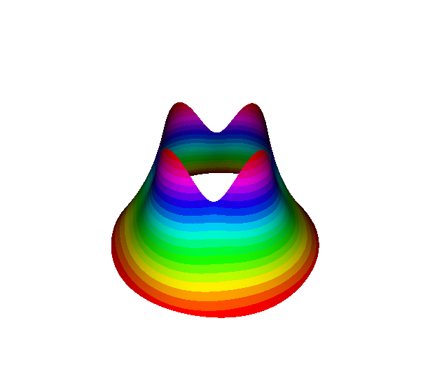
with 15407 elements. We can see that the solution oscillates on the edge of the
obstacle but it is smooth away from the obstacle. This feature is caught by the
algorithm. The mesh is adaptively refined around the obstacle and is coarse
away from the obstacle.
Table 2. Comparison of numerical results using adaptive mesh and uniform
mesh refinements for Example 1.
Adaptive mesh
Uniform mesh
1745
0.4632
3.9693
1745
0.4632
3.9693
2984
0.3256
2.6723
2667
0.3717
3.2365
5559
0.2253
1.9293
5857
0.2494
2.0625
9030
0.1778
1.5054
10630
0.1851
1.5856
15407
0.1384
1.1686
20224
0.1330
1.1257
Figure 2. Quasi-optimality of the a priori and a posteriori error
estimates for Example 1.
Figure 3. The numerical solution of Example 1. (left) the magnitude of the
numerical solution; (left) an adaptively refined mesh with 15407 elements.
Example 2. This example does not have an analytical solution. We consider
a compressional plane incident wave with
the incident direction . The obstacle is U-shaped
and is contained in the rectangular domain . Due to the problem geometry, the
solution contains singularity around the corners of the obstacle. We take . Figure 4 shows the curve of versus
at different frequencies .
It demonstrates that the decay of the a posteriori error estimates are
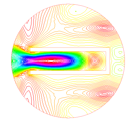
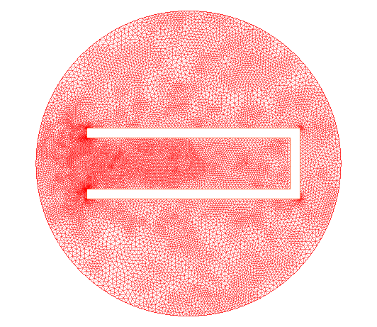
. Figure 5 plots the contour of the
magnitude of the numerical solution and its corresponding mesh by using the
parameters . Again, the algorithm does capture the
solution feature and adaptively refines the mesh around the corners of the
obstacle where the solution displays singularity.
Figure 4. Quasi-optimality of the a posteriori error estimates with
different frequencies for Example 2.
Figure 5. The numerical solution of Example 2. (left) The contour plot of the
magnitude of the solution; (right) an adaptively refined mesh with
12329 elements
6. Conclusion
In this paper, we present an adaptive finite element DtN method for the elastic
obstacle scattering problem. Based on the Helmholtz decomposition, a
new duality argument is developed to obtain the a posteriori error estimate. It
not only takes into account of the finite element discretization error but also
includes the truncation error of the DtN operator. We show that the truncation
error decays exponentially with respect to the truncation parameter. The
posteriori error estimate for the solution of the discrete problem serves as a
basis for the adaptive finite element approximation. Numerical results show that
the proposed method is accurate and effective. This work provides a viable
alternative to the adaptive finite element PML method to solve the elastic
obstacle scattering problem. The method can be applied to solve many other wave
propagation problems where the transparent boundary conditions are used for
open domain truncation. Future work includes extending our analysis to the
adaptive finite element DtN method for solving the three-dimensional elastic
obstacle scattering problem, where a more complicated transparent boundary
condition needs to be considered.
Appendix A Transparent boundary conditions
In this section, we show the transparent boundary conditions for the scalar
potential functions and the displacement of the scattered field
on .
In the exterior domain , the solutions of
the Helmholtz equations (2.5) have the Fourier series expansions in the
polar coordinates:
(A.1)
where is the Hankel function of the first kind with order .
Taking the normal derivative of (A.1), we obtain the transparent
boundary condition for the scalar potentials on :
(A.2)
The polar coordinates are related to the Cartesian coordinates
by with the local
orthonormal basis , where
.
Define a boundary operator for the displacement of the scattered wave
Based on the Helmholtz decomposition (2.5) and the transparent
boundary condition (A.2), it is shown in [33] that the
scattered field satisfies the transparent boundary condition
(A.3)
where
and is a matrix defined by
(A.4)
Here
(A.5)
and
The matrix entries can be further simplied. Recall that
the Hankel function satisfies the Bessel differential equation
Let . For sufficiently large , admits the following
asymptotic property
Proof.
Using the asymptotic expansions of the Hankel functions [43]
we have
A simple calcuation yields that
which completes the proof.
∎
References
[1]
I. Babuška and A. Aziz, Survey Lectures on Mathematical Foundations of the
Finite Element Method, in the Mathematical Foundation of the Finite Element
Method with Application to the Partial Differential Equations, ed. by
A.Aziz, Academic Press, New York, 1973, 5–359.
[2]
I. Babuška and C. Werner, Error estimates for adaptive finite element
computations, SIAM J. Numer. Anal., 15 (1978), 736–754.
[3]
G. Bao, G. Hu, J. Sun, and T. Yin, Direct and inverse elastic scattering from
anisotropic media, J. Math. Pures Appl., 117 (2018), 263–301.
[4]
G. Bao, P. Li, and H. Wu, An adaptive edge element method with perfectly matched
absorbing layers for wave scattering by periodic structures, Math. Comp., 79
(2010), 1–34.
[5]
G. Bao and H. Wu, Convergence analysis of the perfectly matched layer problems
for time harmonic Maxwell’s equations, SIAM J. Numer. Anal., 43 (2005),
2121–2143.
[6]
A. Bayliss and E. Turkel, Radiation boundary conditions for numerical simulation
of waves, Comm. Pure Appl. Math., 33 (1980), 707–725.
[7]
J. P. Berenger, A perfectly matched layer for the absorption of electromagnetic
waves, J. Comput. Phys., 114 (1994), 185–200.
[8]
J. H. Bramble, J. E. Pasciak, and D. Trenev, Analysis of a finite PML
approximation to the three dimensional elastic wave scattering problem, Math.
Comp., 79 (2010), 2079–2101.
[9]
J. Chen and Z. Chen, An adaptive perfectly matched layer technique for 3-D
time-harmonic electromagnetic scattering problems, Math. Comp., 77 (2008),
673–698.
[10]
Z. Chen and H. Wu, An adaptive finite element method with perfectly matched
absorbing layers for the wave scattering by periodic structures, SIAM J.
Numer. Anal., 41 (2003), 799–826.
[11]
Z. Chen and X. Liu, An adaptive perfectly matched layer technique for
time-harmonic scattering problems, SIAM J. Numer. Anal., 43 (2005), 645–671.
[12]
Z. Chen, X. Xiang, and X. Zhang, Convergence of the PML method for elastic wave
scattering problems, Math. Comp., 85 (2016), 2687–2714.
[13]
W. Chew and Q. Liu, Perfectly matched layers for elastodynamics: a new
absorbing boundary condition, J. Comput. Acoust., 4 (1996), 341–359.
[14]
W. Chew and W. Weedon, A 3D perfectly matched medium for modified Maxwell’s
equations with stretched coordinates, Microwave Opt. Techno. Lett., 13
(1994), 599–604.
[15]
P. G. Ciarlet, Mathematical Elasticity, vol. I : Three-Dimensional Elasticity,
Studies in Mathematics and its Applications, North-Holland, Amsterdam, 1988.
[16]
F. Collino and C. Tsogka, Application of the PML absorbing layer model to the
linear elastodynamics problem in anisotropic heterogeneous media, Geophysics,
66 (2001), 294–307.
[17]
D. Colton and R. Kress, Integral Equation Methods in Scattering Theory, Wiley,
New York, 1983.
[18]
B. Engquist and A. Majda, Absorbing boundary conditions for the numerical
simulation of waves, Math. Comp., 31 (1977), 629–651.
[19]
G. K. Gächter and M. J. Grote, Dirichlet-to-Neumann map for
three-dimensional elastic waves, Wave Motion, 37 (2003), 293–311.
[20]
D. Givoli and J. B. Keller, Non-reflecting boundary conditions for elastic
waves, Wave Motion, 12 (1990), 261–279.
[21]
F. D. Hastings, J. B. Schneider, and S. L. Broschat, Application of the
perfectly matched layer (PML) absorbing boundary condition to elastic wave
propagation, J. Acoust. Soc. Am., 100 (1996), 3061–3069.
[22]
F. Hecht, New development in FreeFem++, J. Numer. Math., 20 (2012), 251–265.
[23]
T. Hohage, F. Schmidt, and L. Zschiedrich, Solving time-harmonic scattering
problems based on the pole condition. II: Convergence of the PML method, SIAM J.
Math. Anal., 35 (2003), 547–560.
[24]
M. Grote and J. Keller, On nonreflecting boundary conditions, J. Comput.
Phys., 122 (1995), 231–243.
[25]
X. Jiang, P. Li, J. Lv, and W. Zheng, An adaptive finite element method for the
wave scattering with transparent boundary condition, J. Sci. Comput., 72
(2017), 936–956.
[26]
X. Jiang and P. Li, An adaptive finite element PML method for the
acoustic-elastic interaction in three dimensions, Commun. Comput. Phys.,
22 (2017), 1486–1507.
[27]
X. Jiang, P. Li, J. Lv, Z. Wang, H. Wu, and W. Zheng, An adaptive finite element
DtN method for Maxwell’s equations in biperiodic structures, arXiv:1811.12449.
[28]
X. Jiang, P. Li, and W. Zheng, Numerical solution of acoustic scattering by an
adaptive DtN finite element method, Commun. Comput. Phys., 13 (2013),
1277–1244.
[29]
X. Jiang, P. Li, J. Lv, and W. Zheng, An adaptive finite element PML method for
the elastic wave scattering problem in periodic structures, ESAIM: Math. Model.
Numer. Anal., 51 (2017), 2017–2047.
[30]
X. Jiang, P. Li, J. Lv, and W. Zheng, Convergence of the PML solution for
elastic wave scattering by biperiodic structures, Comm. Math. Sci., 16 (2018),
985–1014.
[31]
D. Komatitsch and J. Tromp, A pefectly matched layer absorbing boundary
condition for the second-order seismic wave equation, Geophys. J. Int., 154
(2003), 146–153.
[32]
L. D. Landau and E. M. Lifshitz, Theory of Elasticity, Theory of Elasticity,
Oxford: Pergamon Press, 1986.
[33]
P. Li, Y. Wang, Z. Wang, and Y. Zhao, Inverse obstacle scattering for elastic
waves, Inverse Problems, 32 (2016), 115018.
[34]
P. Li and X. Yuan, Inverse obstacle scattering for elastic waves in three
dimensions, Inverse Problems and Imaging, to appear.
[35]
M. Grote and C. Kirsch, Dirichlet-to-Neumann boundary conditions for multiple
scattering problems, J. Comput. Phys., 201 (2004), 630–650.
[36]
P. Monk, Finite Element Methods for Maxwell’s Equations, Oxford University
Press, 2003.
[37]
J.-C. Nédélec, Acoustic and Electromagnetic Equations Integral
Representations for Harmonic Problems, Springer-Verlag, New York, 2001.
[38]
L. Scott and S. Zhang, Finite element interpolation of nonsmooth functions
satisfying boundary conditions, Math. Comp., 54 (1990), 483–493.
[39]
A. H. Schatz, An observation concerning Ritz–Galerkin methods with indefinite
bilinear forms, Math. Comp., 28 (1974), 959–962.
[40]
H. Thomas, Radiation boundary conditions for the numerical simulation of
waves, Acta Numer., 8 (1999), 47–106.
[41]
E. Turkel and A. Yefet, Absorbing PML boundary layers for wave-like equations,
Appl. Numer. Math., 27 (1998), 533–557.
[42]
Z. Wang, G. Bao, J. Li, P. Li, and H. Wu, An adaptive finite element method for
the diffraction grating problem with transparent boundary condition, SIAM J.
Numer. Anal., 53 (2015), 1585–1607.
[43]
G.N. Watson, A Treatise on the Theory of Bessel Functions, Cambridge
University Press, 1995.