Protecting quantum correlations in presence of generalised amplitude damping channel: the two-qubit case
Abstract
Any kind of quantum resource useful in different information processing tasks is vulnerable to several types of environmental noise. Here we study the behaviour of quantum correlations such as entanglement and steering in two-qubit systems under the application of the generalised amplitude damping channel and propose two protocols towards preserving them under this type of noise. First, we employ the technique of weak measurement and reversal for the purpose of preservation of correlations. We then show how the evolution under the channel action can be seen as an unitary process. We use the technique of weak measurement and most general form of selective positive operator valued measure (POVM) to achieve preservation of correlations for a significantly large range of parameter values.
I Introduction
Non-local features of quantum correlations enable us to perform various information processing tasks, such as quantum teleportation Bennett et al. 1993, super dense coding Bennett and Wiesner 1992, quantum error correction Shor 1995, device-independent quantum key distribution Bennett and Brassard 1984; Ekert 1991; Branciard et al. 2012. While practically implementing such tasks, there is always an interaction of the concerned quantum system with some noisy environment. Such interactions diminish the quantum correlations present in the state under consideration, in general. So it is one of the most important jobs in any information processing task to preserve the quantum correlations in presence of noisy environment, at least by some amount. This necessitates formulation of protocols for controlling decoherence of a system.
There are various well-known forms of decoherence modelled by qubit channels such as the depolarising channel, dephasing channel, amplitude damping channel (ADC), generalised amplitude damping channel (GADC), and so on Bruß et al. 2000; Schumacher and Nielsen 1996; Srikanth and Banerjee 2008; Fujiwara 2004; Nielsen and Chuang 2002. It is not possible to enhance quantum correlation in two-qubit system by unital operations, whereas for some initial states it might be possible to enhance or generate quantum correlation such as discord when the system passes through some non-unital channel Streltsov et al. 2011. For example, interaction through amplitude damping channel can enhance the teleportation fidelity for a particular class of two-qubit entangled state Badziag et al. 2000; Bandyopadhyay 2002. On the other hand, using the technique of weak measurement, one can protect loss of entanglement Koashi and Ueda 1999; Korotkov and Jordan 2006; Kim et al. 2009; Kim et al. 2012; Heibati et al. 2020, and improve the fidelity of teleportation Pramanik and Majumdar 2013 as well as the secret key rate for certain quantum key distribution protocols Datta et al. 2017, while the interaction is taking place through the ADC.
There exist other ways to protect quantum correlations from environmental noise, such as by employing quantum Zeno effect Misra and Sudarshan 1977; Facchi et al. 2004, frequent unitary interruptions (bang-bang pulse) Viola and Lloyd 1998; Zanardi 1999; Byrd and Lidar 2002; Byrd and Lidar 2003, strong continuous coupling Peres 1980; Schulman 1998; Facchi et al. 2005, etc. In the present work, we focus on the problem of preservation of quantum correlations under the decoherence arising from the action of the generalised amplitude damping channel. Note that all of the aforesaid decoherence control process are dynamical in nature: one needs to follow the dynamics of the system in order to implement each such control process. On the other hand, the environment action, considered in the present work is of static nature and hence the aforesaid decoherence controlling mechanisms will not work, in general, in the case considered here.
In quantum information theory, there exists mainly three types of nonlocal correlations for multipartite systems, namely entanglemet Einstein et al. 1935, steering Schrodinger 1935; Reid 1989; Wiseman et al. 2007; Jones et al. 2007; Skrzypczyk et al. 2014; Gallego and Aolita 2015 and Bell-nonlocality Bell 1964; Clauser et al. 1969; Werner 1989. In 1935, the concept of entanglement was first introduced in context of the famous EPR paradox Einstein et al. 1935. In the same year, this paradox was revisited by Schrödinger and was interpreted with the introduction of another stricter form of quantum correlation for pure states, termed as steerability Schrodinger 1935. Much later, this concept was generalised for mixed states Wiseman et al. 2007; Jones et al. 2007. Meanwhile, John Bell introduced the idea of Bell-nonlocality Bell 1964 which is the strongest form of quantum correlation known so far.
Here, we confine our studies within the first two types of quantum correlations, namely, entanglement and steering. Each of these two correlations decreases under the action of generalised amplitude damping channel acting on one of the qubits, which is a non-unital channel. Now, for the purpose of preservation of non-local correlation, we start with pure (maximally and non-maximally) entangled states, and first employ the technique of weak measurement which has been used in case of the standard ADC Datta et al. 2017.
In the case of weak measurement, as first proposed in Aharonov et al. 1988, the interaction between the system and the apparatus is taken to be very weak, along with two processes termed as pre-selection and post-selection measurementDressel et al. 2014. To use weak measurement as a procedure for preservation of correlations in a quantum state, one has to do the weak measurement, and the reverse weak measurement to be followed at the end of the protocol. The procedure of weak measurement has been used in a huge number of protocols to study different interesting phenomena in quantum theory, such as spin Hall effect Hosten and Kwiat 2008, wave particle duality using cavity-QED experiments Wiseman 2002, superluminal propagation of light Solli et al. 2004; Brunner et al. 2004, direct measurement of the quantum wave function Lundeen et al. 2011, measurement of ultrasmall time delays of light Brunner and Simon 2010, observing Bohmian trajectories of photons Kocsis et al. 2011; Ghose et al. 2001 and also for detection of entanglement with minimal resources Goswami et al. 2019.
Next, to make the technique of preservation of non-local correlations more general for environmental noise, we find the unitary dilation corresponding to the completely positive trace-preserving evolution of the GADC, starting from its known Kraus representation Breuer et al. 2002. After finding the inverse of this unitary, we construct the most general form of operator-sum representation (Kraus representation) of an approximate inverse map, which is not unique. Employing these Kraus operators individually as the elements of a POVM, we show that it is possible to preserve the correlations of the initial state up to certain extents for a broad range of state parameter and damping coefficients.
It should be noted that in all cases here one has to employ selective POVM, as non-selective POVM corresponds to a unitary evolution, and under local unitary it is not possible to generate or enhance any kind of quantum correlation Vedral and Plenio 1998. Although our method (to be described in Sec. (IV) below) may appear to be quite specific towards tackling the noise of GADC, nevertheless, as a method, it has a general appeal in the sense that it can, in principle, be applicable to any noise model - provided we have the prior information about the noise model. (It may be note here that the aforesaid process of addressing decoherence via unitary dilation does not take into account, in general, any driving mechanism, to act on the system using apparatus having support outside of the ancilla Hilbert space. In this sence, our aforesaid approach is a restricted one.) Any physical quantum operation is guided by a completely positive trace preserving (CPTP) map which in turn can be expressed as an unitary dilation. The applicability of unitary dilation is a well discussed topic in literature Buscemi et al. 2003a; Caruso et al. 2011; Buscemi et al. 2003b. Also the implementation of selective POVM is nothing but doing some probabilistic measurements and can also be physically realized Ziman and Bužek 2005.
Our paper is arranged in the following way. After the introduction, we first discuss the preliminary definitions related to our protocol and the technical tools that we will use in the rest of the analysis, in Sec. (II). In Sec. (III), we discuss our first approach for the preservation of quantum correlations using the technique of weak measurement. In the following Sec. (IV), we propose another more general protocol for the preservation of quantum correlations considering GADC as a unitary evolution. In Sec. (V), we summarize our work, and present a brief discussion about some future directions.
II Background
Any quantum state that can be written as a convex mixture of product states of its own subsystems, is termed as a separable state. Now any state that can not be expressed in this form, is an entangled state, i.e. for a bipartite entangled state , one can write,
| (1) |
for any and , the states corresponding to the subsystems and respectively. There are various ways to quantify entanglement in a given biparite state Gühne and Tóth 2009. For the purpose of this problem, we consider concurrence as the measure of entanglement Coffman et al. 2000. Concurrence of a given two-qubit state is defined as
| (2) |
with, , , , being the eigenvalues of the matrix in the descending order, with (, being the Pauli Y-matrix).
Now, let us briefly discuss about another quantum correlation, termed as quantum steering which is a stronger form of quantum correlation than entanglement. In this scenario, one side (say, ) is untrusted i.e., the dimension of the subsystem is completely uncharacterised. If can convince by local operation and classical communication (LOCC), that they are sharing an entangled state, then the state shared between them is said to be a steerable state. Here we consider the steering scenario, in which performs two black-box dichotomic observables (i.e. they can be any two dichotomic observables in any dimension) and and performs two qubit-measurements in mutually unbiased bases, given by and . Then the necessary and sufficient condition for quantum steering Cavalcanti et al. 2015 can be written in terms of an inequality (also termed as ACHSH inequality for steering) as stated below.
| (3) |
with, . Here, and are the possible outcomes () of the dichotomic measurements by and respectively. We will be considering the inequality given in Eq.(3) for the certification of steerability in this paper. Note that the violation of this inequality is necessary and sufficient to certify steering in a two-qubit system.
In this paper, we study the behaviour of the aforesaid two quantum correlations (entanglement and steering) under the application of local environmental noise expressed in the form of generalised amplitude damping. GADC can be obtained by solving the optical master equation in presence of a squeezed thermal bath and this channel describes the effect of environmental dissipation in a finite temperature bath. The Kraus operators of the corresponding channel are given by,
| (4) |
where, is related to the temperature of the heat bath and is the parameter representing the rate of dissipation due to the heat bath action. Note that, for , the Kraus representation in Eq.(4) traces down to that of an ADC, for which the environment is assumed to be at zero temperature. The GADC map acts here on one of the qubits of a two-qubit state
| (5) |
In previous works it has been shown that it is possible to subdue the effect of environmental interaction through ADC by the application of the technique of weak measurement and its reversal Koashi and Ueda 1999; Korotkov and Jordan 2006; Kim et al. 2009; Kim et al. 2012; Pramanik and Majumdar 2013; Datta et al. 2017. In the similar way, in this paper, we first study the effect of weak measurement technique when the environmental interaction is taking place through GADC. Here, before the environmental interaction takes place with the particle in consideration (say, ) of the bipartite system , weak measurement (WM) with a strength is performed on the same. The detector detects the system with probability if and only if the state of is in and hence the measurement operator corresponding to this scenario is given as,
| (6) |
Note that, the matrix in Eq. (6) is singular. Hence this is not effective to implement for the reverse weak measurement. So, for the purpose of weak measurement, we consider the measurement operator corresponding to the scenario when the system is not detected by the measuring apparatus. The measurement operator corresponding to this situation can be evaluated by using the relation, . Hence,
| (7) |
As the matrix in Eq. (7) is a reversible one, application of the inverse of it leads back the system to its original state. According to the our protocol, after the weak measurement is done, the particle in consideration interacts with the environment through the GADC and lastly reverse weak measurement (RWM) is done on the same. The Kraus opearator corresponding to the reverse weak measurement is gievn below.
| (8) |
where, is the strength of the reverse weak measurement (we consider it different from the weak measurement strength to make sure that there is a freedom of choice for different efficiencies of weak and reverse weak measurement).
After the implementation of the technique of weak measurement, now we propose another, our more general approach for the purpose of preservation of steering and entanglement of the bipartite state while interacting with environment through GADC. Here we consider the unitary dilation corresponding to the completely positive trace preserving (CPTP) map described by the GADC. The unitary dilation corresponding to the Kraus operator representation given in Eq.(4), is not unique and can be obtained considering a two-qubit ancilla for the action of GADC on one side of the two-qubit system. The action of this unitary (say, ) on the initial state of system () plus ancilla () gives the state after the environmental interaction has taken place through GADC. In the next step, we find the inverse of this unitary () from which one can find the corresponding Kraus operator representation of the evolution. These individual Kraus operators can be considered as elements of the most general POVM not. Employing the selective POVM obtained corresponding to the inverse map, either before or after the action of the GADC, we study the concurrence and the steerability of the final state.
III Employing the technique of weak measurement
As described in the previous section, here we consider that only one side of the bipartite system is interacting with the environment. We study two cases described in the flowchart given below.
-
.
-
.
where ’s, and are given by Eq. (4), (7) and (8) respectively. Note that comparison of steerability and concurrence between the states and gives the idea about the fact whether the technique of weak measurement is useful for the preservation of quantum correlation. In the whole paper, we consider either pure anti-parallel entangled state () or pure parallel entangled state () in computational basis as the initial state () for all the protocols, where,
| (9) | |||
| (10) |
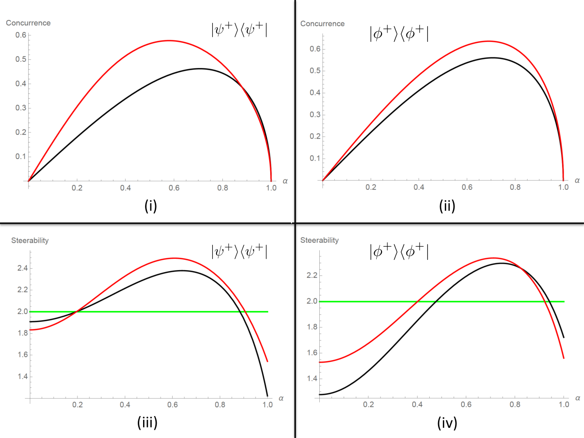
In the above cases one must have , to fulfil the demand of normalisation. We compute the concurrence as well as the magnitude of violation of the analog CHSH inequality as a quantifier for steering. It is evident from Fig.(1), the correlations (entanglement and steering) show a certain amount of improvement for a section of pure states (for some values of state parameter ) under the application of weak measurement technique. Note that the plots in Fig.(1) are corresponding to a particular set of values of the GADC parameters, and . It can be seen that for some other set of values for the channel parameter and , it is possible to preserve both the correlations under the application of weak measurement corresponding to different weak measurement strength and reverse weak measurement strength . But, the range of channel parameters for this technique showing any improvement is quite small.
It may be noted that for a large number of values (though not always for a continuous range) of and this technique is unable to preserve the correlations. In fact, this technique has the capability of functioning for different weak and reverse weak measurement strengths and giving improvement for a rather restrictive set of parameter values of channel and state parameter (one of which is shown in the Fig (1)). On the contrary, for other values of the channel parameter, the state remains un-steerable even after employing weak measurement technique. For example, for and this fact can be observed from Fig (2). So in the next section we propose a more general approach for the preservation of quantum correlation using the selective POVM. This approach is general in the sense that it deals with the unitary dilation of the GADC, which is not unique. This gives us the freedom to choose the suitable POVM that pre serves the correlation maximally.
IV Preserving the correlation considering a unitary dilation of GADC
It is a well-known fact that any quantum channel that corresponds to a physical process can be seen as a CPTP evolution. In this section we try to obtain the unitary dilation of the CPTP evolution corresponding to the GADC and use the same for the purpose of preservation of entanglement and steerability.
IV.1 Motivation behind the approach
Every CPTP map () can be realized via unitary dilation, followed by tracing out the ancillary part: with a fixed state of the ancilla and any state of the system . Such a unitary is not unique even if we allow the dimension of the ancilla to be square of the minimum number of Kraus operators needed to realize . Our aim is to choose such an (as well as ) such that:
i) becomes whenever becomes the identity channel.
ii) is close to a product state of the form where is fixed state of the ancilla.
Condition (ii) guarantees that is close to the initial state . And hence, the reduced state of , after the action of would become close to . Moreover is a CPTP map on . This is the motivation behind adopting the aforesaid approach.
The pertinent question that one needs to answer is whether it is at all possible to satisfy condition (ii) (condition (i) can always be satisfied). Though there exists no general proof of this as such, we consider here (in the next section) two types of such unitaries ’s, and validity of condition (ii) may be tested for these two choices.
IV.2 To find the unitary dilation and its inverse
Let us start by considering a general CPTP map given as , with being the dimensional Hilbert space associated with a given quantum system and represents the set of all bounded linear operators, . It is obvious that has an operator-sum representation (or, Kraus representation) expressed as, ( being a finite positive integer) with the Kraus operators satisfying the condition, . Now, let us consider an ancilla system whose associated Hilbert space has dimension . Let, be an orthonormal basis (ONB) for while be an ONB for . Our aim i s to find a unitary matrix which corresponds to the map such that,
| (11) |
Alternatively, for every (thus, can also be a density matrix of ), one can write,
| (12) |
Note that, for a given CPTP map, its unitary dilation given by the matrix is not unique. The -entry of the matrix can be obtained in the following way,
| (13) | |||||
For a given set of Kraus operators, , ,…, , with the help of Eq. (13), it is possible to obtain information about column vectors of the unitary matrix (with respect to the joint ONB ) and they are given below.
| (14) | |||||
Thus, we obtain an incomplete ONB of the dimensional Hilbert space . At this point, we use the method of basis extension to extend this incomplete ONB given in Eq. (14) to form the complete ONB for and eventually to construct the unitary matrix . The procedure of basis expansion is not unique, but it is restricted by two conditions: i) all the column vectors of should be orthogonal to each other and ii) the individual columns must be normalised. Taking these two constraints into consideration one can construct different f orms of starting from Eq. (14), all of which represents the same CPTP map that we have started with.
Now, let us consider the Kraus representation of GADC (expressed in the computational basis) given in Eq. (4) and the evolution of is given by, Eq. (5). Hence, in this particular scenario of environmental interaction through GADC, we have and . Thus, in this case, the unitary matrix must be of dimension . Following the technique mentioned above in Eq. (13), we find only two columns of the unitary, which are and ,:
| (15) | |||
| (16) |
Using the method of basis expansion, and by taking care of the constraints stated previously, we construct several unitary matrices representing the noisy channel (GADC) in consideration. Note that, from Eq. (4), for , the channel should represent an identity operation. Keeping all these facts in mind, in this work, we concentrate on two separate unitary evolutions corresponding to the GADC which are given in terms of the matrix below.
Note that, in these cases the aforesaid GADC appears as a dynamical process in time (as for example, by solving the optical master equation with the initial state of the heat bath taken to be squeezed vacuum). Our aim is to find out the Kraus operator representation of the quantum channel whose unitary dilation corresponds to the inverse of this unitary evolution. As is unitary, we must have . Now under the action of the inverse unitary evolution , the state of the system at the output end is given by, , where is the state of the system just before the action of the inverse unitary. Now if for be the Kraus operators corresponding to the channel described by the inverse unitary, one must have,
| (35) |
with, for . In fact, if , then , and so,
| (36) | |||||
Using the technique mentioned above, we find out the Kraus operators (, , , ) corresponding to the channel which is given by the inverse of the unitary .
IV.3 Fidelity of the quantum state
We can now consider the entire scenario in the following fashion,
-
.
-
.
Here, represents the action of the inverse map on the evolved state under environmental interaction. Basically, in this case, we consider a two qubit ancilla along with the initial quantum state, and let the whole 4-qubit state pass through the unitary dilation corresponding to the GADC in the following way,
| (37) | |||||
After obtaining the evolved state by tracing out the ancillary qubits, the process of initialization of ancilla is employed and let the whole system pass through the inverse unitary map which corresponds to the reverse effect of the channel action. In this case one may check the closeness of the state with and compare it with the closeness of states and. The fidelity as a quantifier for closeness, is given as,
| (38) |
For the approach of preservation of entanglement and steerability to be successful, implementation of the inverse map on the evolved system’s state and the initialized ancilla, should lead to a high fidelity for a large range of values of the damping channel parameter.
IV.4 To preserve quantum correlation using unitary dilation
Following the procedure, mentioned above, of finding the Kraus operator representation associated to the inverse of the unitary dilation of a quantum channel, here we obtain the set of Kraus operators and corresponding to the unitaries given in Eq. (IV.2) and (IV.2) respectively, which are illustrated below.
and,
Note that, and . Let us now consider that one side (, say) of the bipartite system is interacting with the environment through a GADC and hence we apply the selective POVM constructed from the individual element of the Kraus representaion. In this scenario, we consider two different cases depending upon the order of application of the POVM.
Case I:
-
.
-
.
Case II:
-
.
-
.
For Case I, we comparatively study the concurrence and steerability of the states and , whereas in Case II, the similar protocol has been followed for the states and . In the figures (3), (5) and (5), we provide plots of the concurrence and steerabilty illustrating examples of the above two cases taking initial Bell states. Comparisons with the weak measurement technique discuused earlier, is also provided for the corresponding values of channel parameters.

From the plots, improvement of quantum correlations on the application of POVM can be seen, over the sole interaction with the environment through GADC. This is a more general approach than the approach discussed in the Sec (III) and improvement can be seen over a larger range of values of the damping parameters and in this case, compared to the weak measurement technique. Also, finding the suitable unitary matrix just by the method of basis expansion, one can identify the helpful POVM in protecting the quantum correlation, for a particular damping channel. From Figure (6), the improvement in steerability can be seen for several different values of the channel parameters. It can be observed that the unitary applied after the environmental interaction works well for the chosen set of values of and and for initial state being the parallel Bell state, i.e. . On the other hand, can be chosen for an effective solution for the antiparallel Bell state when applied before the environmental interaction, as can be seen from Fig (5).
The motivation behind introducing the unitary dilation of a quantum channel (acting on ) and the quantum channel (acting on ) whose unitary dilation being , is to nullify the action of . Such a scheme will be completely successful provided it can be guaranteed that is close to for two fixed states and of B. Needless to say, such a condition can not be satisfied, in general. Hence, our method can only recover the quantum correlation of the state partially. There are decoherence controlling models in literature for the noisy channels obtained by solving the optical master equation for thermal bath Misra and Sudarshan 1977; Viola and Lloyd 1998. But for the particular case of GADC, which can be obtained from a squeezed thermal bath, our method of protecting quantum correlations is an effective pr ocedure.
A possible way to choose the unitary dilation – satisfying (i) of Sec(IV.1) and approximately satisfying (ii) of Sec (IV.1)– is the following. Choose in such a way that (a) it satisfies (i), (b) the reduced states of are closed to each other over all choices of the initial states of S, and (c) has minimal entangling power Zanardi et al. 2000. Note that conditions (b) and (c) together (which are not necessarily independent of each other) satisfy condition (ii) above. Also note that, the aforesaid ancilla state may now be chosen (given that satisfies conditions (a), (b), and (c)) to be the average of over all possible choices of the initial states of the system . Needless to say that finding out the unitary dilation , satisfying the conditions (a) - (c), is computationally a challenging task although, as a method, this has a universal character.
V Conclusions
In this paper, we have studied the problem of preserving quantum correlations that are useful in different information processing tasks, under the action of a noisy environment. Here, we choose GADC as the environmental noise and check its effect on entanglement and steerability of an initial pure bipartite state. First, we have employed the technique of weak measurement and reversal and found that a certain amount of improvement could be achieved. But, it can also be seen that this improvement is restricted to some particular values of the damping parameters of the corresponding channel.
We have next introduced another method for the preservation of correlations using a unitary dilation of the operator sum representation of the channel. Interestingly, as the choice of the unitary is not unique, it provides us the freedom to choose the inverse evolution of the unitary, and hence the Kraus operators according to our convenience. Choosing different unitaries and consequently their inverses gives us the scope to extend our scheme over a larger range of the damping parameters, thus improving the quality of preservation. Note that in the present paper we have dealt with two particular unitaries corresponding the Kraus representation of GADC for the illustration of our approach. However, it is possible to construct other unitaries taking the conditions of orthogonality and normalisation into account. Also, there can be other protocols using partial inversion of CPTP channels leading to improvement in terms of fidelity Karimipour et al. 2020.
As a future direction, this method can be applied to other noisy channels and the choice of the unitary can be made suitably in order to generate an optimal scheme for protecting quantum correlations under the action of different noisy environments. On the other hand, another interesting and useful approach towards the preservation of correlations would be to find the optimized solution for the problem. It may be noted that the considered prescription gives us a wide opportunity to choose between numerous unitary dilation corresponding to a given channel as it is not unique. Hence, it could be more helpful to choose the unitary corresponding to which the highest fidelity can be obtained for a particular scenario. Also, one has to keep in mind that the ancillary state that would be traced out after the unitary evolution, should be as near as possible to the initially taken ancillary state. In this way we would introduce the least amount of correlation to the ancillary system which gives us the opportunity to find the unitary that performs better in preserving the correlation in the main system under consideration.
Acknowledgements.
SG1 would like to acknowledge Sagnik Chakraborty and Samyadeb Bhattacharya for helpful discussions. SG2 would like to thankfully acknowledge the hospitality of S. N. Bose National Centre for Basic Sciences during his visits in the recent past during which part of the work was done. ASM acknowledges Project no. DST/ICPS/QuEST/2018/98 of Department of Science and Technology, Government of India.References
- Bennett et al. (1993) C. H. Bennett, G. Brassard, C. Crépeau, R. Jozsa, A. Peres, and W. K. Wootters, Physical review letters 70, 1895 (1993).
- Bennett and Wiesner (1992) C. H. Bennett and S. J. Wiesner, Physical review letters 69, 2881 (1992).
- Shor (1995) P. W. Shor, Phys. Rev. A 52, R2493 (1995).
- Bennett and Brassard (1984) C. H. Bennett and G. Brassard (1984) pp. 175–179.
- Ekert (1991) A. K. Ekert, Phys. Rev. Lett. 67, 661 (1991).
- Branciard et al. (2012) C. Branciard, E. G. Cavalcanti, S. P. Walborn, V. Scarani, and H. M. Wiseman, Phys. Rev. A 85, 010301 (R) (2012).
- Bruß et al. (2000) D. Bruß, L. Faoro, C. Macchiavello, and G. M. Palma, Journal of Modern Optics 47, 325 (2000).
- Schumacher and Nielsen (1996) B. Schumacher and M. A. Nielsen, Phys. Rev. A 54, 2629 (1996).
- Srikanth and Banerjee (2008) R. Srikanth and S. Banerjee, Phys. Rev. A 77, 012318 (2008).
- Fujiwara (2004) A. Fujiwara, Phys. Rev. A 70, 012317 (2004).
- Nielsen and Chuang (2002) M. A. Nielsen and I. Chuang, “Quantum computation and quantum information,” (2002).
- Streltsov et al. (2011) A. Streltsov, H. Kampermann, and D. Bruß, Phys. Rev. Lett. 107, 170502 (2011).
- Badziag et al. (2000) P. Badziag, M. Horodecki, P. Horodecki, and R. Horodecki, Phys. Rev. A 62, 012311 (2000).
- Bandyopadhyay (2002) S. Bandyopadhyay, Phys. Rev. A 65, 022302 (2002).
- Koashi and Ueda (1999) M. Koashi and M. Ueda, Phys. Rev. Lett. 82, 2598 (1999).
- Korotkov and Jordan (2006) A. N. Korotkov and A. N. Jordan, Phys. Rev. Lett. 97, 166805 (2006).
- Kim et al. (2009) Y.-S. Kim, Y.-W. Cho, Y.-S. Ra, and Y.-H. Kim, Optics express 17, 11978 (2009).
- Kim et al. (2012) Y.-S. Kim, J.-C. Lee, O. Kwon, and Y.-H. Kim, Nature Physics 8, 117 (2012).
- Heibati et al. (2020) O. Heibati, A. Mani, and V. Karimipour, arXiv preprint arXiv:2003.01341 (2020).
- Pramanik and Majumdar (2013) T. Pramanik and A. Majumdar, Phys. Lett. A 377, 3209 (2013).
- Misra and Sudarshan (1977) B. Misra and E. G. Sudarshan, Journal of Mathematical Physics 18, 756 (1977).
- Facchi et al. (2004) P. Facchi, D. Lidar, and S. Pascazio, Phys. Rev. A 69, 032314 (2004).
- Viola and Lloyd (1998) L. Viola and S. Lloyd, Phys. Rev. A 58, 2733 (1998).
- Zanardi (1999) P. Zanardi, Phys. Lett. A 258, 77 (1999).
- Byrd and Lidar (2002) M. S. Byrd and D. A. Lidar, Quantum Information Processing 1, 19 (2002).
- Byrd and Lidar (2003) M. S. Byrd and D. A. Lidar, Phys. Rev. A 67, 012324 (2003).
- Peres (1980) A. Peres, American Journal of Physics 48, 931 (1980).
- Schulman (1998) L. Schulman, Phys. Rev. A 57, 1509 (1998).
- Facchi et al. (2005) P. Facchi, S. Tasaki, S. Pascazio, H. Nakazato, A. Tokuse, and D. Lidar, Phys. Rev. A 71, 022302 (2005).
- Einstein et al. (1935) A. Einstein, B. Podolsky, and N. Rosen, Phys. Rev. 47, 777 (1935).
- Schrodinger (1935) E. Schrodinger, Mathematical Proceedings of the Cambridge Philosophical Society 31, 555 (1935).
- Reid (1989) M. D. Reid, Phys. Rev. A 40, 913 (1989).
- Wiseman et al. (2007) H. M. Wiseman, S. J. Jones, and A. C. Doherty, Phys. Rev. Lett. 98, 140402 (2007).
- Jones et al. (2007) S. J. Jones, H. M. Wiseman, and A. C. Doherty, Phys. Rev. A 76, 052116 (2007).
- Skrzypczyk et al. (2014) P. Skrzypczyk, M. Navascués, and D. Cavalcanti, Phys. Rev. Lett. 112, 180404 (2014).
- Gallego and Aolita (2015) R. Gallego and L. Aolita, Phys. Rev. X 5, 041008 (2015).
- Bell (1964) J. S. Bell, Physics Physique Fizika 1, 195 (1964).
- Clauser et al. (1969) J. F. Clauser, M. A. Horne, A. Shimony, and R. A. Holt, Phys. Rev. Lett. 23, 880 (1969).
- Werner (1989) R. F. Werner, Phys. Rev. A 40, 4277 (1989).
- Datta et al. (2017) S. Datta, S. Goswami, T. Pramanik, and A. Majumdar, Phys. Lett. A 381, 897 (2017).
- Aharonov et al. (1988) Y. Aharonov, D. Z. Albert, and L. Vaidman, Phys. Rev. Lett. 60, 1351 (1988).
- Dressel et al. (2014) J. Dressel, M. Malik, F. M. Miatto, A. N. Jordan, and R. W. Boyd, Rev. Mod. Phys. 86, 307 (2014).
- Hosten and Kwiat (2008) O. Hosten and P. Kwiat, Science 319, 787 (2008).
- Wiseman (2002) H. M. Wiseman, Phys. Rev. A 65, 032111 (2002).
- Solli et al. (2004) D. R. Solli, C. F. McCormick, R. Y. Chiao, S. Popescu, and J. M. Hickmann, Phys. Rev. Lett. 92, 043601 (2004).
- Brunner et al. (2004) N. Brunner, V. Scarani, M. Wegmüller, M. Legré, and N. Gisin, Physical review letters 93, 203902 (2004).
- Lundeen et al. (2011) J. S. Lundeen, B. Sutherland, A. Patel, C. Stewart, and C. Bamber, Nature 474, 188 (2011).
- Brunner and Simon (2010) N. Brunner and C. Simon, Phys. Rev. Lett. 105, 010405 (2010).
- Kocsis et al. (2011) S. Kocsis, B. Braverman, S. Ravets, M. J. Stevens, R. P. Mirin, L. K. Shalm, and A. M. Steinberg, Science 332, 1170 (2011).
- Ghose et al. (2001) P. Ghose, A. Majumdar, S. Guha, and J. Sau, Physics Letters A 290, 205 (2001).
- Goswami et al. (2019) S. Goswami, S. Chakraborty, S. Ghosh, and A. S. Majumdar, Phys. Rev. A 99, 012327 (2019).
- Breuer et al. (2002) H.-P. Breuer, F. Petruccione, et al., The theory of open quantum systems (Oxford University Press on Demand, 2002).
- Vedral and Plenio (1998) V. Vedral and M. B. Plenio, Physical Review A 57, 1619 (1998).
- Buscemi et al. (2003a) F. Buscemi, G. D’Ariano, P. Perinotti, and M. Sacchi, Physics Letters A 314, 374 (2003a).
- Caruso et al. (2011) F. Caruso, J. Eisert, V. Giovannetti, and A. S. Holevo, Phys. Rev. A 84, 022306 (2011).
- Buscemi et al. (2003b) F. Buscemi, G. M. D’Ariano, and M. F. Sacchi, Phys. Rev. A 68, 042113 (2003b).
- Ziman and Bužek (2005) M. Ziman and V. Bužek, Phys. Rev. A 72, 022343 (2005).
- Gühne and Tóth (2009) O. Gühne and G. Tóth, Physics Reports 474, 1 (2009).
- Coffman et al. (2000) V. Coffman, J. Kundu, and W. K. Wootters, Phys. Rev. A 61, 052306 (2000).
- Cavalcanti et al. (2015) E. G. Cavalcanti, C. J. Foster, M. Fuwa, and H. M. Wiseman, JOSA B 32, A74 (2015).
- (61) Note here that the reduced CPTP map (acting on ), formed out of , is not necessarily the inverse of the given GADC (even if such an inverse map exists). This would have been the case, if under a suitable choice of an initial state of the ancilla , the reduced state of becomes close to the initial state before applying the GADC .
- Zanardi et al. (2000) P. Zanardi, C. Zalka, and L. Faoro, Phys. Rev. A 62, 030301 (2000).
- Karimipour et al. (2020) V. Karimipour, F. Benatti, and R. Floreanini, Phys. Rev. A 101, 032109 (2020).