Unsupervised Learning
of Probabilistic Diffeomorphic Registration
for Images and Surfaces

Although the method presented in this paper applies to a multitude of deformable representations, we choose to work with diffeomorphisms, and in particular with a stationary velocity field representation [5]. Diffeomorphic deformations are differentiable and invertible, and thus preserve topology. Let $\boldsymbol{\phi}:\mathbb{R}^{3}\rightarrow\mathbb{R}^{3}$ represent the deformation that maps the coordinates from one image to coordinates in another image. In our implementation, the deformation field is defined through the following ordinary differential equation (ODE):

where $\boldsymbol{\phi}^{(0)}=Id$ is the identity transformation and $t$ is time. We integrate the stationary velocity field $\boldsymbol{v}$ over $t=[0,1]$ to obtain the final registration field $\boldsymbol{\phi}^{(1)}$ [53].

While we implement and evaluate several numerical integration techniques, we find scaling and squaring to be most efficient, and we briefly review the technique here [4]. The integration of a stationary ODE represents a one-parameter subgroup of diffeomorphisms. In group theory, $\boldsymbol{v}$ is a member of the Lie algebra and is exponentiated to produce $\boldsymbol{\phi}^{(1)}$, which is a member of the Lie group: $\boldsymbol{\phi}^{(1)}=\text{exp}(\boldsymbol{v})$. From the properties of one-parameter subgroups, for any scalars $t$ and $t^{\prime}$, $\exp((t+t^{\prime})\boldsymbol{v})=\exp(t\boldsymbol{v})\circ\exp(t^{\prime}\boldsymbol{v})$, where $\circ$ is a composition map associated with the Lie group. Starting from $\boldsymbol{\phi}^{(1/2^{T})}=\boldsymbol{p}+\boldsymbol{v}(\boldsymbol{p})/2^{T}$ where $\boldsymbol{p}$ is a map of spatial locations, we use the recurrence $\boldsymbol{\phi}^{(1/2^{t-1})}=\boldsymbol{\phi}^{(1/2^{t})}\circ\boldsymbol{\phi}^{(1/2^{t})}$ to obtain $\boldsymbol{\phi}^{(1)}=\boldsymbol{\phi}^{(1/2)}\circ\boldsymbol{\phi}^{(1/2)}$. $T$ is chosen so that $\boldsymbol{v}/2^{T}$ is very small.

We model the prior probability of the parametrization $\boldsymbol{z}$ as:

where $\mathcal{N}(\cdot;\boldsymbol{\mu},\boldsymbol{\Sigma})$ is the multivariate normal distribution with mean $\boldsymbol{\mu}$ and covariance $\boldsymbol{\Sigma}$. Our work applies to a wide range of representations $\boldsymbol{z}$. For example, $\boldsymbol{z}$ could be a dense displacement field, or a low-dimensional embedding of the displacement field. In this paper, we let $\boldsymbol{z}$ be a stationary velocity field that specifies a diffeomorphism through the ODE (1). We let $\boldsymbol{L}=\boldsymbol{D}-\boldsymbol{A}$ be the Laplacian of a neighborhood graph defined on the voxel grid, where $\boldsymbol{D}$ is the graph degree matrix, and $\boldsymbol{A}$ is a voxel neighbourhood adjacency matrix. We encourage spatial smoothness of the velocity field $\boldsymbol{z}$ by setting $\boldsymbol{\Sigma}_{z}^{-1}=\boldsymbol{\Lambda}_{z}=\lambda\boldsymbol{L}$, where $\boldsymbol{\Lambda}_{z}$ is a precision matrix and $\lambda$ denotes a parameter controlling the scale of the velocity field $\boldsymbol{z}$.

We let $\boldsymbol{f}$ be a noisy observation of warped image $\boldsymbol{m}$:

where $\sigma_{I}^{2}$ captures the variance of additive image noise.

We aim to estimate the posterior registration probability $p(\boldsymbol{z}|\boldsymbol{f};\boldsymbol{m})$. Using this, we can obtain the most likely registration field $\boldsymbol{\phi}_{\boldsymbol{z}}$ for a new image pair $(\boldsymbol{f},\boldsymbol{m})$ via MAP estimation, along with an estimate of velocity field variance at each voxel. Figure 1 provides a graphical representation of our model.

Given our assumptions, computing the posterior probability $p(\boldsymbol{z}|\boldsymbol{f};\boldsymbol{m})$ is intractable. We use a variational approach, and introduce an approximate posterior probability $q_{\boldsymbol{\psi}}(\boldsymbol{z}|\boldsymbol{f};\boldsymbol{m})$ parametrized by $\boldsymbol{\psi}$. We minimize the KL divergence

which yields the negative of the variational lower bound of the model evidence [39]. We model the approximate posterior $q_{\boldsymbol{\psi}}(\boldsymbol{z}|\boldsymbol{f};\boldsymbol{m})$ as a multivariate normal:

where we let $\boldsymbol{\Sigma}_{z|m,f}$ be diagonal. To understand the effects of this assumption, we explore a non-diagonal covariance in a later section. The statistics $\boldsymbol{\mu}_{z|m,f}$ and the diagonal of $\boldsymbol{\Sigma}_{z|m,f}$ can be interpreted as the voxel-wise mean and variance, respectively.

We estimate $\boldsymbol{\mu}_{z|m,f}$, and $\boldsymbol{\Sigma}_{z|m,f}$ using a convolutional neural network $\text{def}_{\boldsymbol{\psi}}(\boldsymbol{f},\boldsymbol{m})$ parameterized by $\boldsymbol{\psi}$, as described in the next section. We learn parameters $\boldsymbol{\psi}$ by optimizing the variational lower bound (4) using stochastic gradient methods. Specifically, for each image pair $(\boldsymbol{f},\boldsymbol{m})$ and sample $\boldsymbol{z}_{k}\sim q_{\psi}(\boldsymbol{z}|\boldsymbol{f};\boldsymbol{m})$, we compute $\boldsymbol{m}\circ\boldsymbol{\phi}_{z_{k}}$, with the resulting loss (detailed derivation in supplementary material):

where $K$ is the number of samples used to approximate the expectation. The first term encourages image $\boldsymbol{f}$ to be similar to the warped image $\boldsymbol{m}\circ\boldsymbol{\phi}_{z_{k}}$. The second term encourages the posterior to be close to the prior $p(\boldsymbol{z})$. Although the variational covariance $\boldsymbol{\Sigma}_{z|m,f}$ is diagonal, the last term spatially smoothes the mean, which can be seen by expanding  $\boldsymbol{\mu}_{z|m,f}^{T}\boldsymbol{\Lambda}_{z}\boldsymbol{\mu}_{z|m,f}=\frac{\lambda}{2}\sum\sum_{j\in N(I)}(\boldsymbol{\mu}[i]-\boldsymbol{\mu}[j])^{2}$, where $N(i)$ are the neighbors of voxel $i$. We treat $\sigma^{2}$ and $\lambda$ as fixed hyper-parameters that we investigate in our experiments, and use $K=1$.

We design the network  $\text{def}_{\boldsymbol{\psi}}(\boldsymbol{f},\boldsymbol{m})$ that takes as input $\boldsymbol{f}$ and $\boldsymbol{m}$ and outputs $\boldsymbol{\mu}_{z|m,f}$ and $\boldsymbol{\Sigma}_{z|m,f}$, based on a 3D UNet-style architecture [60]. The network includes a convolutional layer with 32 filters, four downsampling layers with 64 convolutional filters and a stride of two, and three upsampling convolutional layers with 64 filters. We only upsample three times to predict the velocity field (and following integration steps) at every two voxels, to enable these operations to fit in current GPU card memory.

To enable unsupervised learning of parameters $\boldsymbol{\psi}$ using (6), we must form $\boldsymbol{m}\circ\boldsymbol{\phi}_{z}$ and compute the data term. We first implement a layer that samples a new $\boldsymbol{z}_{k}\sim\mathcal{N}(\boldsymbol{\mu}_{z|m,f},\boldsymbol{\Sigma}_{z|m,f})$ using the “re-parameterization trick" [39]: $\boldsymbol{z}_{k}=\boldsymbol{\mu}_{z|m,f}+\sqrt{\boldsymbol{\Sigma}_{z|m,f}}\boldsymbol{r}$, where $\boldsymbol{r}$ is a sample from the standard normal: $\boldsymbol{r}\sim\mathcal{N}(0,\boldsymbol{I})$.

Given $\boldsymbol{z}_{k}$, we need to compute $\boldsymbol{\phi}_{z_{k}}=\exp(\boldsymbol{z}_{k})$ as described in the introduction. We propose vector integration layers using scaling and squaring operations. Specifically, scaling and squaring operations involve compositions within the neural network architecture using a differentiable spatial transformation operation. Given two 3D vector fields $\boldsymbol{a}$ and $\boldsymbol{b}$, for each voxel $p$ this operation computes $(\boldsymbol{a}\circ\boldsymbol{b})(p)=\boldsymbol{a}(\boldsymbol{b}(p))$, a non-integer voxel location $\boldsymbol{b}(\boldsymbol{p})$ in $\boldsymbol{a}$, using linear interpolation. Starting with $\boldsymbol{\phi}^{(1/2^{T})}=\boldsymbol{p}+\boldsymbol{z}_{k}/2^{T}$, we compute $\boldsymbol{\phi}^{(1/2^{t-1})}=\boldsymbol{\phi}^{(1/2^{t})}\circ\boldsymbol{\phi}^{(1/2^{t})}$ recursively using these operations T times, leading to $\boldsymbol{\phi}^{(1)}\triangleq\boldsymbol{\phi}_{z_{k}}=\exp(\boldsymbol{z}_{k})$. In our experiments, we extensively analyze the effect of the step size $T$ on the runtime of the network, the accuracy of the registration, and the regularity of the deformation. We also implement vector integration layers using quadrature and ODE solvers, and in the experiments show that these are significantly slower and can require significant memory.

Finally, we warp volume $\boldsymbol{m}$ according to the computed diffeomorphic field $\boldsymbol{\phi}_{z_{k}}$ using a spatial transform layer.

In summary, the network takes as input images $\boldsymbol{f}$ and $\boldsymbol{m}$, computes statistics $\boldsymbol{\mu}_{z|m,f}$ and $\boldsymbol{\Sigma}_{z|m,f}$, samples a new velocity field $\boldsymbol{z}_{k}\sim\mathcal{N}(\boldsymbol{\mu}_{k},\boldsymbol{\Sigma}_{k})$, computes a diffeomorphic $\boldsymbol{\phi}_{z_{k}}$ and warps $\boldsymbol{m}$. Since all the steps are designed to be differentiable, we learn the network parameters using stochastic gradient descent-based methods. This network results in three outputs, $\boldsymbol{\mu}_{z|m,f},\boldsymbol{\Sigma}_{z|m,f}$ and $\boldsymbol{m}\circ\boldsymbol{\phi}_{z_{k}}$, which are used in the model loss (6). The framework is summarized in Figure 2.

Given learned parameters, we approximate registration of a new scan pair $(\boldsymbol{f},\boldsymbol{m})$ using $\boldsymbol{\phi}_{\hat{z}_{k}}$. We first obtain the most likely velocity field $\hat{\boldsymbol{z}}_{k}$ using

by evaluating the neural network $\text{def}_{\psi}(\boldsymbol{f},\boldsymbol{m})$. We then compute $\boldsymbol{\phi}_{\hat{z}_{k}}$ using the scaling and squaring based integration, altogether requiring less than a second on a GPU. We highlight that at test time, the diagonal covariance $\boldsymbol{\Sigma}_{z|m,f}$ is not used, however it enables an estimation of the deformation uncertainty. Analysis of uncertainty is beyond the scope of this paper, and is an interesting avenue for future study.

Using a stationary velocity field representation, computing the inverse deformation field $\boldsymbol{\phi}^{-1}_{\boldsymbol{z}}$ can be achieved by integrating the negative of the velocity field: $\boldsymbol{\phi}^{-1}_{\boldsymbol{z}}=\boldsymbol{\phi}_{-\boldsymbol{z}}$, since $\boldsymbol{\phi}_{\boldsymbol{z}}\circ\boldsymbol{\phi}_{-\boldsymbol{z}}=\exp(\boldsymbol{z})\circ\exp(-\boldsymbol{z})=\exp(\boldsymbol{z}-\boldsymbol{z})=Id$ [5, 52]. This enables the computation of both fields inside one efficient network when desired.

We implement our method as part of the VoxelMorph package [9], available online at http://voxelmorph.csail.mit.edu, using neuron [20] and Keras [16] with a Tensorflow [1] backend. We use a learning rate of $1e-4$ for the Adam optimizer [38], a batch size of 1 due to memory constraints, and Glorot uniform initialization for the convolution weights. We use a single sample ($K=1$), which has been shown to lead to useful gradients for optimization while maintaining the memory footprint and implementation complexity low [39]. For large volumes, the number of samples is often constrained by the available GPU memory.

In various instances, anatomical segmentation maps for specific structures of interest may also be available with some of the training images. Recent papers have demonstrated that the use of segmentations can help in registration [10, 34]. Here, we show that our proposed model naturally extends to handle surfaces, enabling the use of segmentations during training within the same principled framework.

We focus on the case where one anatomical structure is segmented in the image. Given a segmentation map where each voxel is assigned the desired anatomical label or background, we extract the anatomical surface and let $\boldsymbol{s}_{\boldsymbol{f}}$ represent the $N$ surface coordinates of the anatomical structure for image $\boldsymbol{f}$, which can be stored as an $N\times 3$ matrix. Given the diffeomorphism $\boldsymbol{\phi}_{z}$ in the previous section, we model each surface location $\boldsymbol{s}_{f}[n]$, as formed by displacing a matching surface location $\boldsymbol{s}_{m}[n]$ according to $\boldsymbol{\phi}_{z}$, and adding (spatial) displacement noise:

where the composition $\boldsymbol{s}_{\boldsymbol{m}}\circ\boldsymbol{\phi}_{\boldsymbol{z}}$ warps surface coordinates.

Given both images and segmentation maps during training, we extract surfaces of the desired structure and aim to estimate the posterior probability $p(\boldsymbol{z}|\boldsymbol{f},\boldsymbol{s}_{\boldsymbol{f}};\boldsymbol{m},\boldsymbol{s}_{\boldsymbol{m}})$. As before, we use a variational approximation. Since segmentation maps, and hence surfaces, are usually derived from images, we assume that images are sufficient to approximate the posterior: $q(\boldsymbol{z}|\boldsymbol{f},\boldsymbol{s}_{\boldsymbol{f}};\boldsymbol{m},\boldsymbol{s}_{\boldsymbol{m}})=q_{\boldsymbol{\psi}}(\boldsymbol{z}|\boldsymbol{f};\boldsymbol{m})$. As before, we minimize the KL divergence between the true and approximate posterior (derived in supplementary material):

and arrive at the loss function:

Compared to the original model loss (6), the additional third term encourages the deformation $\boldsymbol{\phi}_{z_{k}}$ to warp the moving surface close to the fixed surface $\boldsymbol{s}_{f}$. As described in the generative model (8), this requires corresponding surface points in $\boldsymbol{s}_{\boldsymbol{f}}$ and $\boldsymbol{s}_{\boldsymbol{m}}$. However, these correspondences are not available in practice, as segmentations are provided independently for each image. Therefore, the third term cannot be computed directly.

We propose an approximation of the surface term using surface distance transforms. Let $\text{sd}(x,\boldsymbol{s})$ be a surface distance function, which for location $x$ returns the Euclidean distance to the closest surface point in $\boldsymbol{s}$ (Figure 3Left).¹¹ 1 Function $\text{sd}(x,\boldsymbol{s})$ is a generating function for a distance transform image for the surface $\boldsymbol{s}$, by evaluating it at every grid point $x$ Noting that for two surfaces $\boldsymbol{a}$ and $\boldsymbol{b}$, $\sum_{n}\text{sd}(\boldsymbol{a}[n],\boldsymbol{b})\neq\sum_{n}\text{sd}(\boldsymbol{b}[n],\boldsymbol{a})$ due to potential asymmetries in the surfaces (see Figure 3Right), we approximate the distance $\|\boldsymbol{s}_{\boldsymbol{f}}-\boldsymbol{s}_{\boldsymbol{m}}\circ\boldsymbol{\phi}_{z_{k}}\|^{2}$ by computing $\text{sd}(\cdot,\cdot)$ in both directions:

We implement this function efficiently using distance transforms. Specifically, to compute $\text{sd}(\boldsymbol{s}_{\boldsymbol{m}}[n]\circ\boldsymbol{\phi}_{z},\boldsymbol{s}_{\boldsymbol{f}})$, we first pre-compute distance transforms for the (fixed) given structure $\boldsymbol{s}_{f}$. We then sample $100,000$ points along $\boldsymbol{s}_{m}$, which we find to be sufficient to estimate accurate measures along the surface. We warp (move) them according to the deformation $\boldsymbol{\phi}_{z}$, and compute the distance transform of $\boldsymbol{s}_{f}$ at these locations. We take advantage of our diffeomorphic representation that enables computing the inverse $\boldsymbol{\phi}_{z}^{-1}$ efficiently within the network to similarly compute $\text{sd}(\boldsymbol{s}_{\boldsymbol{f}}[n]\circ\boldsymbol{\phi}_{z}^{-1},\boldsymbol{s}_{\boldsymbol{m}})$.

In summary, since to compute the posterior approximation $q_{\boldsymbol{\psi}}(\boldsymbol{z}|\boldsymbol{f};\boldsymbol{m})$ the neural network takes as input only the images $\boldsymbol{f}$ and $\boldsymbol{m}$, images alone are required at test time. Given a diffeomorphism $\boldsymbol{\phi}_{z_{k}}$, at training time the network uses both a warped image and a warped surface to evaluate the quality of the registration.

This model can also be used to register two surfaces when the images themselves are not available. The only modelling change required is removing the image likelihood terms and using the variational approximation $q_{\boldsymbol{\psi}}(\boldsymbol{z}|\boldsymbol{S}_{\boldsymbol{f}};\boldsymbol{S}_{\boldsymbol{m}})$, which uses the segmentation maps $\boldsymbol{S}_{m}$ and $\boldsymbol{S}_{f}$ as input. Surface-only registration is beyond the scope of this paper, and we leave it for future work. However, registration with images and surfaces is described here as an example of possible extensions of the model, and surface-only registration is beyond the scope of this paper.

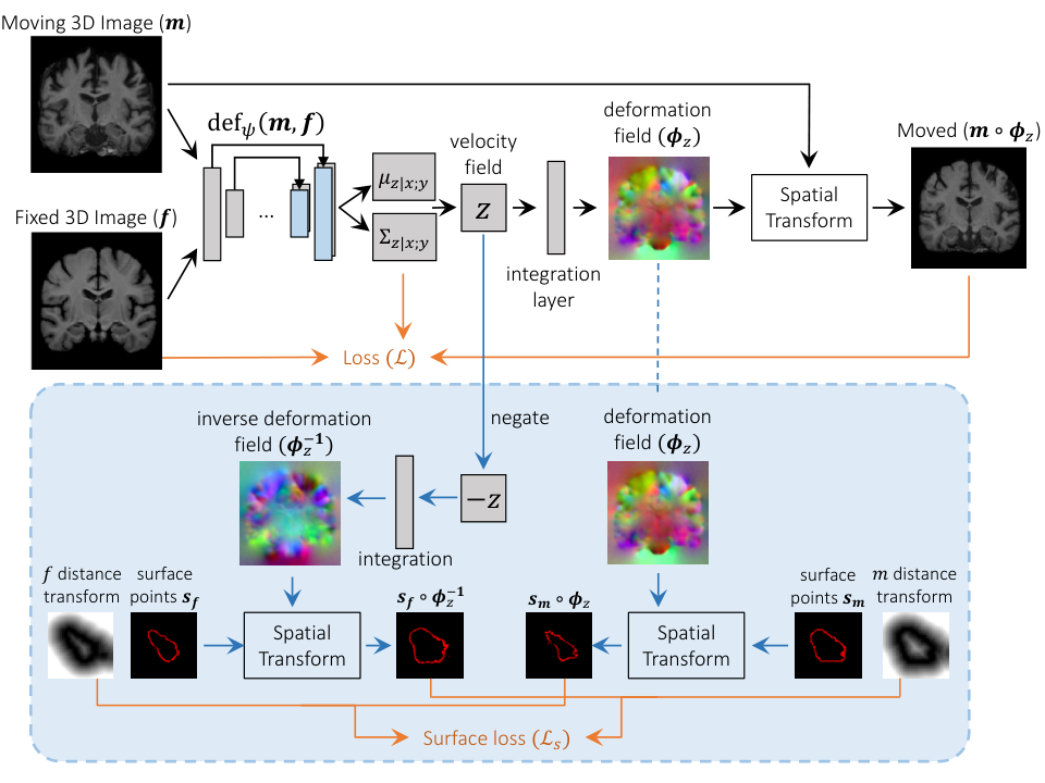
The complete neural network framework, including the surface loss, is illustrated in supplemental Figure 12.

Approximating the velocity field covariance $\boldsymbol{\Sigma}_{z|m,f}$ using a diagonal matrix is a strong assumption that ignores spatial smoothness. As seen in (6), the spatially-smooth prior $p(\boldsymbol{z})$ encourages a smooth mean velocity field $\boldsymbol{\mu}_{z|m,f}$, but samples $\boldsymbol{z}_{k}\sim\mathcal{N}(\boldsymbol{\mu}_{z|m,f},\boldsymbol{\Sigma}_{z|m,f})$ might still be noisy. In this section, we investigate the effects of this restriction, by providing a model expansion that computes a less restrictive covariance. In our experiments below, we analyze the effects of these different approximations.

To evaluate the effects of the diagonal covariance, we explore a second approximation $\boldsymbol{\Sigma}_{z|m,f}=\boldsymbol{C}_{\sigma_{c}}\boldsymbol{G}\boldsymbol{G}^{T}\boldsymbol{C}_{\sigma_{c}}^{T}$ where $\boldsymbol{G}$ is a diagonal matrix returned by the neural network and $\boldsymbol{C}_{\sigma_{c}}$ is a fixed smoothing convolution matrix. Specifically, for each row of $\boldsymbol{C}_{\sigma_{c}}$ we create a flattened Gaussian smoothing kernel centered at a particular voxel, such that $\boldsymbol{C}_{\sigma_{c}}\boldsymbol{w}$ is equivalent to 3D convolution of image $\boldsymbol{w}$ by a gaussian filter with variance $\sigma_{c}^{2}$. We choose $\sigma_{c}$ such that the smoothing operation matches the scale of the prior $p(\boldsymbol{z})$ determined by $\lambda$: $\frac{1}{\sqrt{2\pi\sigma_{c}^{3/2}}}=(\lambda*6)^{-1}$.

During training, sampling from the posterior is achieved using the reparametrization trick: $\boldsymbol{z}_{k}=\boldsymbol{\mu}_{z|m,f}+\boldsymbol{C}_{\sigma_{c}}\boldsymbol{D}\boldsymbol{r}$, where $\boldsymbol{r}$ is a sample from the standard normal. Intuitively, compared to the diagonal $\boldsymbol{\Sigma}_{z|m,f}$ approximation, this sampling procedure smoothes the term $\boldsymbol{D}\boldsymbol{r}$ before adding the mean $\boldsymbol{\mu}_{z|m,f}$.

In our experiments, we show that this approximation yields smoother velocity fields during training, and the effect diminishes with higher $\lambda$ values. However, the resulting deformation fields are diffeomorphic and accurate for both approximations, demonstrating that the diagonal covariance approximation is sufficient when working with diffeomorphisms.

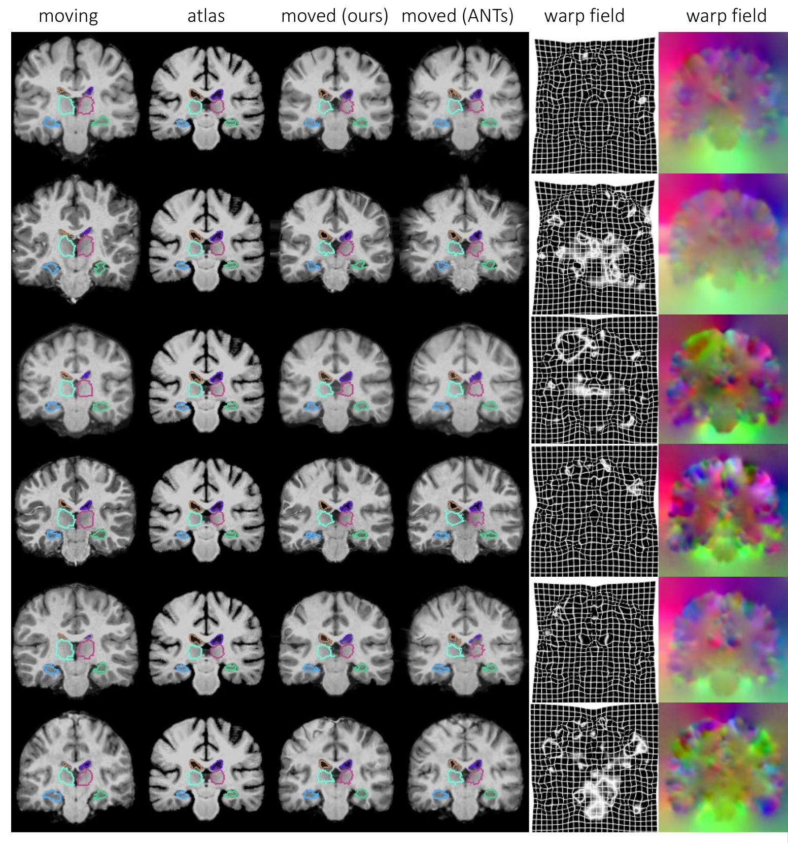
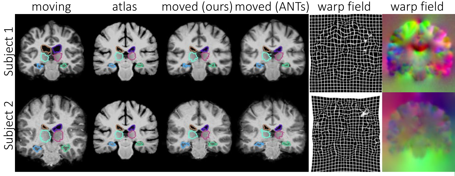
Table 1 provides a summary of the results on the held-out test set. Figure 5 and supplementary material Figure 13 show representative results. Figure 4 illustrates Dice results on several anatomical structures. For better visualization, we combine the same structures from the two hemispheres, such as the left and right hippocampus. Our algorithm, VoxelMorph-diff, achieve state-of-the-art Dice results and runtimes, but produces diffeomorphic registration fields (nearly no folding voxels per scan) in a probabilistic framework.

All methods achieve comparable Dice results on each structure and overall, except the supervised method. Despite training the latter on 650 subjects, we found that the supervised network leads to more diffeomorphic deformations than the training deformations, but results in a slight loss in Dice score. Learning-based methods require a fraction of the baseline runtimes to register two images: less than a second on a GPU, and less than a minute and a half on a CPU. Runtimes were computed for an NVIDIA TitanX GPU and a Intel Xeon (E5-2680) CPU, and exclude preprocessing common to all methods.

Our method outputs positive Jacobians at nearly all voxels, which we analyze in more detail in a later section. For VoxelMorph-diff, we find that for most scans, the deformation fields result in zero folding voxels. Very few volumes lead to a few or tens of grouped folding voxels, leading to a population average of less than a folding voxel per test scan. In contrast, the deformation fields resulting from the baseline methods contain a few thousand locations of non-positive Jacobians for each scan (Table 1), usually grouped in clusters. This may be alleviated with increased spatial regularization or more optimization iterations, but this in turn leads to a drop in performance on the Dice metric or even longer runtimes. The table also shows that, at the presented settings, all methods result in an average Jacobian determinant close to $1$, with VoxelMorph-diff yielding smoothness statistics nearly identical to those given by NiftyReg, indicate smooth deformations.

In this section, we evaluate the generative surface model. We demonstrate the use of anatomical segmentation alongside images during training, and refer to this model as VoxelMorph-Surf. We focus on the setting where one structure of interest is available during training, and learn separate networks for the left white matter, gray matter, ventricle, thalamus and hippocampus. Our goal is to analyze how the additional surface model terms affect the accuracy and regularity of resulting deformations.

Figure 7 illustrates the behaviour of the model with respect to the hyper-parameter $\sigma_{s}$ on the validation set. For a range of $\sigma_{s}$ values, we find a significant improvement in terms of Dice for the desired structure. For very small values of $\sigma_{s}$, the training becomes unstable leading to poor generalization. A very large $\sigma_{s}$ value leads to the model ignoring the surface term. Since the Dice scores are comparable in the range $\sigma_{c}\in[0.5,2]$, for the rest of this section we use $\sigma_{s}=2$, which exhibits slightly fewer folding voxels ($\leq 5$ compared to $\sim 20$ for $\sigma_{c}=1$).

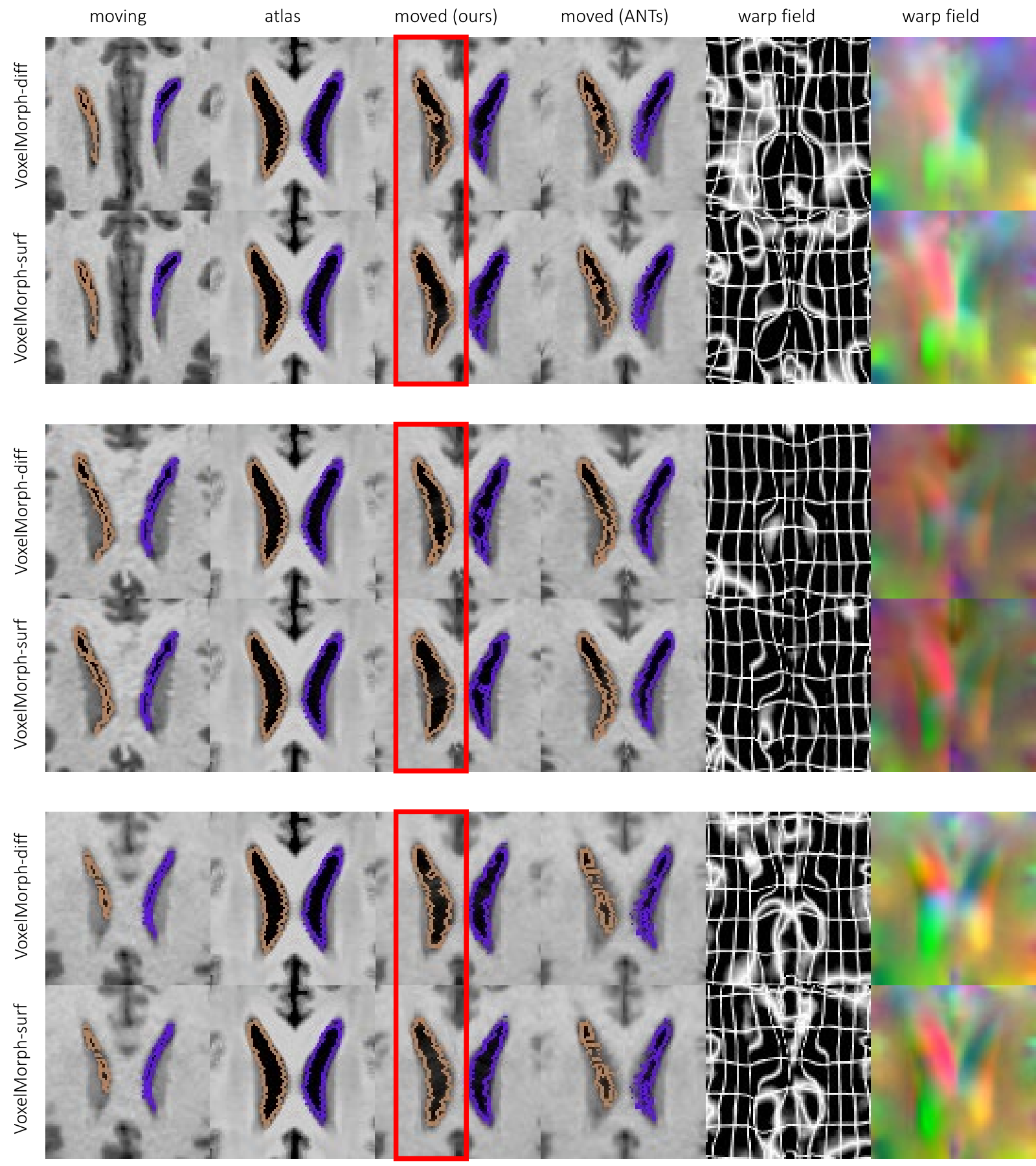
Figure 6 demonstrates the improvement on the test set in terms of Euclidean surface distance and Dice, compared to the image-only registration model VoxelMorph-diff. VoxelMorph-surf improves significantly in all measures for most desired structures. Additionally, Table 2 illustrates that with increased accuracy in both metrics, the number of folding voxels in the entire volume increases only very slightly (to an average 3.5 voxels per volume), which remains orders of magnitude fewer than the baseline methods (Table 1). Figure 14 in the supplementary material illustrates example results.

In summary, the principled joint diffeomorphic model enables the use of surfaces during training which dramatically improves registration near a given structure while preserving desired deformation properties. For example, given hippocampus surfaces at training, registration using VoxelMorph-Surf improves Dice by $\sim 9$ points over VoxelMorph-diff, improves maximum surface distance by more than three voxels, and preserving diffeomorphisms (less than three folding voxels per scan).

Using the facts that $\log|\boldsymbol{\Lambda}_{z}|$ is constant, $\log|\boldsymbol{\Sigma}_{z|m,f}|=\text{tr}\log\boldsymbol{\Sigma}_{z|m,f}$, and $\text{tr}(\boldsymbol{\Lambda}_{z}\boldsymbol{\Sigma}_{z|m,f})=\text{tr}((\lambda\boldsymbol{D}-\boldsymbol{A})\boldsymbol{\Sigma}_{z|m,f})=\text{tr}(\lambda\boldsymbol{D}\boldsymbol{\Sigma}_{z|m,f})$, and approximating the expectation with $K$ samples $z_{k}\sim q_{z}$, we obtain

We derive the variational lower bound and loss for the generative surface model. We start by minimizing the KL divergence between the true and approximate posteriors:

where in $\star$ we used the assumptions that the fixed image is independent of anatomical surfaces given the moving image and the deformation, and the fixed surface is independent of either image given the moving surface and the deformation. Following this variational lower bound, the loss follows the previous section closely (see (13)), with the additional term:

Combining this term with (12), and approximating expectations with $k$ samples leads to the final loss (10):

References

- [1] Martín Abadi, Ashish Agarwal, Paul Barham, Eugene Brevdo, Zhifeng Chen, Craig Citro, Greg S Corrado, Andy Davis, Jeffrey Dean, Matthieu Devin, et al. Tensorflow: Large-scale machine learning on heterogeneous distributed systems. arXiv preprint arXiv:1603.04467, 2016.
- [2] Dror Aiger, Niloy J Mitra, and Daniel Cohen-Or. 4-points congruent sets for robust pairwise surface registration. In ACM transactions on graphics (TOG), volume 27, page 85. Acm, 2008.
- [3] A Amir-Khalili, G Hamarneh, R Zakariaee, I Spadinger, and R Abugharbieh. Propagation of registration uncertainty during multi-fraction cervical cancer brachytherapy. Physics in Medicine & Biology, 62(20):8116, 2017.
- [4] Vincent Arsigny, Olivier Commowick, Xavier Pennec, and Nicholas Ayache. A log-euclidean framework for statistics on diffeomorphisms. In International Conference on Medical Image Computing and Computer-Assisted Intervention, pages 924–931. Springer, 2006.
- [5] J. Ashburner. A fast diffeomorphic image registration algorithm. Neuroimage, 38(1):95–113, 2007.
- [6] J. Ashburner and K. Friston. Voxel-based morphometry-the methods. Neuroimage, 11:805–821, 2000.
- [7] Brian B Avants, Charles L Epstein, Murray Grossman, and James C Gee. Symmetric diffeomorphic image registration with cross-correlation: evaluating automated labeling of elderly and neurodegenerative brain. Medical image analysis, 12(1):26–41, 2008.
- [8] R. Bajcsy and S. Kovacic. Multiresolution elastic matching. Computer Vision, Graphics, and Image Processing, 46:1–21, 1989.
- [9] Guha Balakrishnan, Amy Zhao, Mert R Sabuncu, John Guttag, and Adrian V Dalca. An unsupervised learning model for deformable medical image registration. In Proceedings of the IEEE Conference on Computer Vision and Pattern Recognition, pages 9252–9260, 2018.
- [10] Guha Balakrishnan, Amy Zhao, Mert R Sabuncu, John Guttag, and Adrian V Dalca. Voxelmorph: A learning framework for deformable medical image registration. arXiv preprint arXiv:1809.05231, 2019.
- [11] M Faisal Beg, Michael I Miller, Alain Trouvé, and Laurent Younes. Computing large deformation metric mappings via geodesic flows of diffeomorphisms. Int. J. Comput. Vision, 61:139–157, 2005.
- [12] Paul J Besl and Neil D McKay. Method for registration of 3-d shapes. In Sensor Fusion IV: Control Paradigms and Data Structures, volume 1611, pages 586–607. International Society for Optics and Photonics, 1992.
- [13] Xiaohuan Cao, Jianhua Yang, Jun Zhang, Dong Nie, Minjeong Kim, Qian Wang, and Dinggang Shen. Deformable image registration based on similarity-steered cnn regression. In International Conference on Medical Image Computing and Computer-Assisted Intervention, pages 300–308. Springer, 2017.
- [14] Yan Cao, Michael I Miller, Raimond L Winslow, and Laurent Younes. Large deformation diffeomorphic metric mapping of vector fields. IEEE transactions on medical imaging, 24(9):1216–1230, 2005.
- [15] Can Ceritoglu, Kenichi Oishi, Xin Li, Ming-Chung Chou, Laurent Younes, Marilyn Albert, Constantine Lyketsos, Peter CM van Zijl, Michael I Miller, and Susumu Mori. Multi-contrast large deformation diffeomorphic metric mapping for diffusion tensor imaging. Neuroimage, 47(2):618–627, 2009.
- [16] François Chollet. Keras. https://github.com/fchollet/keras, 2015.
- [17] Alexander Dagley, Molly LaPoint, Willem Huijbers, Trey Hedden, Donald G McLaren, Jasmeer P Chatwal, Kathryn V Papp, Rebecca E Amariglio, Deborah Blacker, Dorene M Rentz, et al. Harvard aging brain study: dataset and accessibility. NeuroImage, 2015.
- [18] Adrian V. Dalca, Guha Balakrishnan, John Guttag, and Mert R. Sabuncu. Unsupervised learning for fast probabilistic diffeomorphic registration. In Medical Image Computing and Computer Assisted Intervention (MICCAI), pages 729–738, Cham, 2018. Springer.
- [19] Adrian V Dalca, Andreea Bobu, Natalia S Rost, and Polina Golland. Patch-based discrete registration of clinical brain images. In MICCAI-PATCHMI Patch-based Techniques in Medical Imaging. Springer, 2016.
- [20] Adrian V Dalca, John Guttag, and Mert R Sabuncu. Anatomical priors in convolutional networks for unsupervised biomedical segmentation. In Proceedings of the IEEE Conference on Computer Vision and Pattern Recognition, pages 9290–9299, 2018.
- [21] Christos Davatzikos. Spatial transformation and registration of brain images using elastically deformable models. Computer Vision and Image Understanding, 66(2):207–222, 1997.
- [22] Bob D de Vos, Floris F Berendsen, Max A Viergever, Hessam Sokooti, Marius Staring, and Ivana Išgum. A deep learning framework for unsupervised affine and deformable image registration. Medical image analysis, 52:128–143, 2019.
- [23] Bob D de Vos, Floris F Berendsen, Max A Viergever, Marius Staring, and Ivana Išgum. End-to-end unsupervised deformable image registration with a convolutional neural network. In DLMIA, pages 204–212. Springer, 2017.
- [24] A. Di Martino et al. The autism brain imaging data exchange: towards a large-scale evaluation of the intrinsic brain architecture in autism. Molecular psychiatry, 19(6):659–667, 2014.
- [25] Lee R. Dice. Measures of the amount of ecologic association between species. Ecology, 26(3):297–302, 1945.
- [26] Stanley Durrleman. Statistical models of currents for measuring the variability of anatomical curves, surfaces and their evolution. PhD thesis, Université Nice Sophia Antipolis, 2010.
- [27] B. Fischl. Freesurfer. Neuroimage, 62(2):774–781, 2012.
- [28] B. Glocker, N. Komodakis, G. Tziritas, N. Navab, and N. Paragios. Dense image registration through mrfs and efficient linear programming. Medical image analysis, 12(6):731–741, 2008.
- [29] Randy L Gollub, Jody M Shoemaker, Margaret D King, Tonya White, Stefan Ehrlich, Scott R Sponheim, Vincent P Clark, Jessica A Turner, Bryon A Mueller, Vince Magnotta, et al. The MCIC collection: a shared repository of multi-modal, multi-site brain image data from a clinical investigation of schizophrenia. Neuroinformatics, 11(3):367–388, 2013.
- [30] Mattias P Heinrich, Mark Jenkinson, Michael Brady, and Julia A Schnabel. Mrf-based deformable registration and ventilation estimation of lung ct. IEEE transactions on medical imaging, 32(7):1239–1248, 2013.
- [31] Mattias P Heinrich, Ivor JA Simpson, BartŁomiej W Papież, Michael Brady, and Julia A Schnabel. Deformable image registration by combining uncertainty estimates from supervoxel belief propagation. Medical image analysis, 27:57–71, 2016.
- [32] Monica Hernandez, Matias N Bossa, and Salvador Olmos. Registration of anatomical images using paths of diffeomorphisms parameterized with stationary vector field flows. International Journal of Computer Vision, 85(3):291–306, 2009.
- [33] Avram J Holmes, Marisa O Hollinshead, Timothy M O’Keefe, Victor I Petrov, Gabriele R Fariello, Lawrence L Wald, Bruce Fischl, Bruce R Rosen, Ross W Mair, Joshua L Roffman, et al. Brain genomics superstruct project initial data release with structural, functional, and behavioral measures. Scientific data, 2, 2015.
- [34] Yipeng Hu, Marc Modat, Eli Gibson, Nooshin Ghavami, Ester Bonmati, Caroline M Moore, Mark Emberton, J Alison Noble, Dean C Barratt, and Tom Vercauteren. Label-driven weakly-supervised learning for multimodal deformable image registration. In Biomedical Imaging (ISBI 2018), 2018 IEEE 15th International Symposium on, pages 1070–1074. IEEE, 2018.
- [35] Yipeng Hu, Marc Modat, Eli Gibson, Wenqi Li, Nooshin Ghavami, Ester Bonmati, Guotai Wang, Steven Bandula, Caroline M Moore, Mark Emberton, et al. Weakly-supervised convolutional neural networks for multimodal image registration. Medical image analysis, 49:1–13, 2018.
- [36] Max Jaderberg, Karen Simonyan, and Andrew Zisserman. Spatial transformer networks. In Advances in neural information processing systems, pages 2017–2025, 2015.
- [37] Sarang C Joshi and Michael I Miller. Landmark matching via large deformation diffeomorphisms. IEEE transactions on image processing, 9(8):1357–1370, 2000.
- [38] Diederik P Kingma and Jimmy Ba. ADAM: A method for stochastic optimization. arXiv preprint arXiv:1412.6980, 2014.
- [39] D.P. Kingma and M. Welling. Auto-encoding variational bayes. arXiv:1312.6114, 2013.
- [40] Arno Klein, Jesper Andersson, Babak A Ardekani, John Ashburner, Brian Avants, Ming-Chang Chiang, Gary E Christensen, D Louis Collins, James Gee, Pierre Hellier, et al. Evaluation of 14 nonlinear deformation algorithms applied to human brain mri registration. Neuroimage, 46(3):786–802, 2009.
- [41] Julian Krebs, Hervé e Delingette, Boris Mailhé, Nicholas Ayache, and Tommaso Mansi. Learning a probabilistic model for diffeomorphic registration. IEEE transactions on medical imaging, 2019.
- [42] Julian Krebs et al. Robust non-rigid registration through agent-based action learning. In Medical Image Computing and Computer-Assisted Intervention (MICCAI), pages 344–352, Cham, 2017. Springer International Publishing.
- [43] Julian Krebs, Tommaso Mansi, Boris Mailhé, Nicholas Ayache, and Hervé Delingette. Unsupervised probabilistic deformation modeling for robust diffeomorphic registration. In Deep Learning in Medical Image Analysis and Multimodal Learning for Clinical Decision Support, pages 101–109. Springer, 2018.
- [44] H. Li and Y. Fan. Non-rigid image registration using fully convolutional networks with deep self-supervision. arXiv preprint arXiv:1709.00799, 2017.
- [45] Daniel S Marcus, Tracy H Wang, Jamie Parker, John G Csernansky, John C Morris, and Randy L Buckner. Open access series of imaging studies (oasis): cross-sectional mri data in young, middle aged, nondemented, and demented older adults. Journal of cognitive neuroscience, 19(9):1498–1507, 2007.
- [46] Kenneth Marek, Danna Jennings, Shirley Lasch, Andrew Siderowf, Caroline Tanner, Tanya Simuni, Chris Coffey, Karl Kieburtz, Emily Flagg, Sohini Chowdhury, et al. The parkinson progression marker initiative (ppmi). Progress in neurobiology, 95(4):629–635, 2011.
- [47] Michael I Miga, Tuhin K Sinha, David M Cash, Robert L Galloway, and Robert J Weil. Cortical surface registration for image-guided neurosurgery using laser-range scanning. IEEE Transactions on medical Imaging, 22(8):973–985, 2003.
- [48] Michael P Milham, Damien Fair, Maarten Mennes, Stewart HMD Mostofsky, et al. The ADHD-200 consortium: a model to advance the translational potential of neuroimaging in clinical neuroscience. Frontiers in systems neuroscience, 6:62, 2012.
- [49] Michael I Miller, M Faisal Beg, Can Ceritoglu, and Craig Stark. Increasing the power of functional maps of the medial temporal lobe by using large deformation diffeomorphic metric mapping. Proceedings of the National Academy of Sciences, 102(27):9685–9690, 2005.
- [50] Marc Modat, David M Cash, Pankaj Daga, Gavin P Winston, John S Duncan, and Sébastien Ourselin. Global image registration using a symmetric block-matching approach. Journal of Medical Imaging, 1(2):024003, 2014.
- [51] Marc Modat, Gerard R Ridgway, Zeike A Taylor, Manja Lehmann, Josephine Barnes, David J Hawkes, Nick C Fox, and Sébastien Ourselin. Fast free-form deformation using graphics processing units. Computer methods and programs in biomedicine, 98(3):278–284, 2010.
- [52] Marc Modat, Ivor JA Simpson, Manual Jorge Cardoso, David M Cash, Nicolas Toussaint, Nick C Fox, and Sébastien Ourselin. Simulating neurodegeneration through longitudinal population analysis of structural and diffusion weighted mri data. Medical Image Computing and Computer-Assisted Intervention, LNCS 8675:57–64, 2014.
- [53] Cleve Moler and Charles Van Loan. Nineteen dubious ways to compute the exponential of a matrix, twenty-five years later. SIAM review, 45(1):3–49, 2003.
- [54] Marc Niethammer, Roland Kwitt, and Francois-Xavier Vialard. Metric learning for image registration. arXiv preprint arXiv:1904.09524, 2019.
- [55] Kenichi Oishi, Andreia Faria, Hangyi Jiang, Xin Li, Kazi Akhter, Jiangyang Zhang, John T Hsu, Michael I Miller, Peter CM van Zijl, Marilyn Albert, et al. Atlas-based whole brain white matter analysis using large deformation diffeomorphic metric mapping: application to normal elderly and alzheimer’s disease participants. Neuroimage, 46(2):486–499, 2009.
- [56] Xavier Pennec, Pascal Cachier, and Nicholas Ayache. Understanding the "demon’s algorithm": 3d non-rigid registration by gradient descent. pages 597–605, 1999.
- [57] Gheorghe Postelnicu, Lilla Zollei, and Bruce Fischl. Combined volumetric and surface registration. IEEE transactions on medical imaging, 28(4):508–522, 2008.
- [58] Petter Risholm, Firdaus Janoos, Isaiah Norton, Alex J Golby, and William M Wells III. Bayesian characterization of uncertainty in intra-subject non-rigid registration. Medical image analysis, 17(5):538–555, 2013.
- [59] Marc-Michel Rohé, Manasi Datar, Tobias Heimann, Maxime Sermesant, and Xavier Pennec. SVF-Net: Learning deformable image registration using shape matching. In MICCAI, pages 266–274. Springer, 2017.
- [60] O. Ronneberger et al. U-net: Convolutional networks for biomedical image segmentation. In MICCAI, pages 234–241. Springer, 2015.
- [61] Daniel Rueckert, Luke I Sonoda, Carmel Hayes, Derek LG Hill, Martin O Leach, and David J Hawkes. Nonrigid registration using free-form deformation: Application to breast mr images. IEEE Transactions on Medical Imaging, 18(8):712–721, 1999.
- [62] D. Shen and C. Davatzikos. Hammer: Hierarchical attribute matching mechanism for elastic registration. IEEE Trans. Med. Imag., 21(11):1421–1439, 2002.
- [63] Ivor JA Simpson, Mark W Woolrich, Jesper LR Andersson, Adrian R Groves, and Julia A Schnabel. A probabilistic non-rigid registration framework using local noise estimates. In 2012 9th IEEE International Symposium on Biomedical Imaging (ISBI), pages 688–691. IEEE, 2012.
- [64] Hessam Sokooti, Bob de Vos, Floris Berendsen, Boudewijn PF Lelieveldt, Ivana Išgum, and Marius Staring. Nonrigid image registration using multi-scale 3d convolutional neural networks. In MICCAI, pages 232–239, Cham, 2017. Springer.
- [65] R. Sridharan, A.V. Dalca, K.M. Fitzpatrick, L. Cloonan, A. Kanakis, O. Wu, K.L. Furie, J. Rosand, N.S. Rost, and P. Golland. Quantification and analysis of large multimodal clinical image studies: Application to stroke. In International Workshop on Multimodal Brain Image Analysis, pages 18–30. Springer International Publishing, 2013.
- [66] J.P. Thirion. Image matching as a diffusion process: an analogy with maxwell’s demons. Medical Image Analysis, 2(3):243–260, 1998.
- [67] Tom Vercauteren et al. Diffeomorphic demons: Efficient non-parametric image registration. NeuroImage, 45(1):S61–S72, 2009.
- [68] Xiao Yang, Roland Kwitt, Martin Styner, and Marc Niethammer. Quicksilver: Fast predictive image registration–a deep learning approach. NeuroImage, 158:378–396, 2017.
- [69] BT Thomas Yeo, Mert R Sabuncu, Tom Vercauteren, Daphne J Holt, Katrin Amunts, Karl Zilles, Polina Golland, and Bruce Fischl. Learning task-optimal registration cost functions for localizing cytoarchitecture and function in the cerebral cortex. IEEE transactions on medical imaging, 29(7):1424–1441, 2010.
- [70] Miaomiao. Zhang, Ruizhi. Liao, Adrian V Dalca, Esra A Turk, Jie Luo, P Ellen Grant, and Polina Golland. Frequency diffeomorphisms for efficient image registration. In International Conference on Information Processing in Medical Imaging, pages 559–570. Springer, 2017.
Supplementary Material
Derivation of Main Loss
Using the facts that is constant, , and , and approximating the expectation with samples , we obtain