跳到论文正文
W Papers独立论文阅读器 arXiv:1903.03296 论文正文 计算阅读时间 · 0%
引用这篇论文根据当前论文元数据生成,正式投稿前建议核对。


License: arXiv.org perpetual non-exclusive license
arXiv:1903.03296v1 [math.NA] 08 Mar 2019

A third order exponential time differencing numerical scheme for no-slope-selection epitaxial thin film model with energy stability

Kelong Cheng Thanks: School of Science, Southwest University of Science and Technology, Mianyang, Sichuan 621010, P. R. China (zhengkelong@swust.edu.cn)    Zhonghua Qiao Thanks: Department of Applied Mathematics, The Hong Kong Polytechnic University, Hung Hom, Kowloon, Hong Kong (zqiao@polyu.edu.hk)    Cheng Wang Thanks: Department of Mathematics, The University of Massachusetts, North Dartmouth, MA 02747, USA (Corresponding Author: cwang1@umassd.edu)
Abstract

In this paper we propose and analyze a (temporally) third order accurate exponential time differencing (ETD) numerical scheme for the no-slope-selection (NSS) equation of the epitaxial thin film growth model, with Fourier pseudo-spectral discretization in space. A linear splitting is applied to the physical model, and an ETD-based multistep approximation is used for time integration of the corresponding equation. In addition, a third order accurate Douglas-Dupont regularization term, in the form of −A​Δ​t2​ϕ0​(LN)​ΔN2​(un+1−un)-A{\Delta t}^{2}\phi_{0}(L_{N})\Delta_{N}^{2}(u^{n+1}-u^{n}), is added in the numerical scheme. A careful Fourier eigenvalue analysis results in the energy stability in a modified version, and a theoretical justification of the coefficient AA becomes available. As a result of this energy stability analysis, a uniform in time bound of the numerical energy is obtained. And also, the optimal rate convergence analysis and error estimate are derived in details, in the ℓ∞​(0,T,Hh1)∩ℓ2​(0,T,Hh3)\ell^{\infty}(0,T;H_{h}^{1})\cap\ell^{2}(0,T;H_{h}^{3}) norm, with the help of a careful eigenvalue bound estimate, combined with the nonlinear analysis for the NSS model. This convergence estimate is the first such result for a third order accurate scheme for a gradient flow. Some numerical simulation results are presented to demonstrate the efficiency of the numerical scheme and the third order convergence. The long time simulation results for ε=0.02\varepsilon=0.02 (up to T=3×10⁵T=3\times 10^{5}) have indicated a logarithm law for the energy decay, as well as the power laws for growth of the surface roughness and the mound width. In particular, the power index for the surface roughness and the mound width growth, created by the third order numerical scheme, is more accurate than those produced by certain second order energy stable schemes in the existing literature.

Key words.   epitaxial thin film growth, slope selection, exponential time differencing, energy stability, optimal rate convergence analysis, aliasing error

AMS Subject Classification   35K30, 35K55, 65L06, 65M12, 65M70, 65T40

1 Introduction

In this article we consider an epitaxial thin film growth equation, which corresponds to the gradient flow associated with the following energy functional

E⁡(u):=∫Ω(−12​ln⁡(1+|∇u|2)+ε22​|Δ​u|2)​dx,E(u):=\int_{\Omega}\left(-\frac{1}{2}\ln(1+|\nabla u|^{2})+\frac{\varepsilon^{2}}{2}|\Delta u|^{2}\right)\mbox{d}\textbf{x}, (1.1)

where Ω=(0,Lx)×(0,Ly)\Omega=(0,L_{x})\times(0,L_{y}), u:Ω→ℝu:\Omega\rightarrow\mathbb{R} is a periodic height function, and ε\varepsilon is a constant. In more details, the first non-quadratic term represents the Ehrlich-Schwoebel (ES) effect, according to which migrating adatoms must overcome a higher energy barrier to stick to a step from an upper rather than from a lower terrace [12, 27, 28, 41]. This results in an uphill atom current in the dynamics and the steepening of mounds in the film. The second term, which is quadratic, but of higher-order, represents the isotropic surface diffusion effect [28, 36]. In turn, the chemical potential becomes the following variational derivative of the energy

μ:=δu​E=∇⋅(∇u1+|∇u|2)+ε2​Δ2​u,\mu:=\delta_{u}E=\nabla\cdot\left(\frac{\nabla u}{1+|\nabla u|^{2}}\right)+\varepsilon^{2}\Delta^{2}u, (1.2)

and the no-slope-selection (NSS) equation stands for the L2L^{2} gradient flow

∂tu=−μ=−∇⋅(∇u1+|∇u|2)−ε2Δ2u.\partial_{t}u=-\mu=-\nabla\cdot\left(\frac{\nabla u}{1+|\nabla u|^{2}}\right)-\varepsilon^{2}\Delta^{2}u. (1.3)

In the small-slope regime, where |∇u|2≪1|\nabla u|^{2}\ll 1, (1.3) may be approximated as

∂tu=∇⋅(|∇u|2∇u)−Δu−ε2Δ2u,\partial_{t}u=\nabla\cdot\left(|\nabla u|^{2}\nabla u\right)-\Delta u-\varepsilon^{2}\Delta^{2}u\ , (1.4)

with the energy functional given by

E⁡(u)=∫Ω(14​(|∇u|2−1)2+ε22​|Δ​u|2)​dx.E(u)=\int_{\Omega}\left(\frac{1}{4}(|\nabla u|^{2}-1)^{2}+\frac{\varepsilon^{2}}{2}|\Delta u|^{2}\right)\mbox{d}\textbf{x}. (1.5)

This model is referred to as the slope-selection (SS) equation [25, 26, 28, 36]. A solution to (1.4) exhibits pyramidal structures, where the faces of the pyramids have slopes |∇u|≈1|\nabla u|\approx 1; meanwhile, the no-slope-selection equation (1.3) exhibits mound-like structures, and the slopes of which (on an infinite domain) may grow unbounded [28, 44]. On the other hand, both solutions have up-down symmetry in the sense that there is no way to distinguish a hill from a valley. This can be altered by adding adsorption/desorption or other dynamics.

In [28], the global in time well-posedness for two nonlinear models of epitaxial thin film epitaxy, with or without slope selection, was established. And also, the gradient bound and the energy asymptotic law for the SS and NSS equations have been studied in [26, 29, 33], as ε→0\varepsilon\to 0. In addition, the large-system asymptotic form of the minimum energy and the magnitude of gradients of energy-minimizing surfaces for epitaxial growth models are analyzed in [27], with infinite or finite ES barrier. Specially, for the case of a finite ES effect (corresponding to the model in this article), the well-posedness of the initial-boundary-value problem is proved and the bounds for the scaling laws of interface width, surface slope and energy are obtained.

There have been many efforts to devise and analyze numerical schemes for both the SS and NSS equations; see the related references [8, 28, 37, 40, 46], etc. In particular, the numerical schemes with high order accuracy and energy stability have been of great interests, due to the long time nature of the gradient flow coarsening process. Among the energy stable numerical approaches, the idea of convex splitting has attracted many attentions. For the epitaxial thin film growth models, the first such work was reported in [44], in which the authors studied unconditionally energy stable schemes, based on the convex-concave decomposition of the energy, motivated by Eyre’s pioneering work [13]. Some other related developments on the energy stable schemes for the MBE models could be found in [5, 7, 14, 21, 32, 34, 35, 38, 39, 42, 47], etc. In particular, it is worthy of mentioning the works [5, 34], in which the authors proposed linear numerical schemes for the NSS equation, with first and second order temporal accuracy orders, respectively, so that the energy stability could be established at a theoretical level. In fact, the following subtle fact has played an essential role in the nonlinear energy stability analysis: in spite of its complicated form in the denominator, the nonlinear term in the NSS equation (1.3) has automatically bounded higher order derivatives in the L∞L^{\infty} norm. In addition, extensive convergence analysis works have been undertaken for these various energy stable numerical schemes, for both the SS and NSS equations.

On the other hand, it is observed that, a theoretical analysis of a (temporally) third order accurate numerical scheme for the gradient equations remains an open problem. In this article, we propose and analyze a (temporally) third order accurate numerical scheme for the NSS equation (1.3), based on the exponential time differencing (ETD) temporal algotirhm, combined with Fourier pseudo-spectral approximation in space. In general, an exact integration of the linear part of the NSS equation is involved in the ETD-based scheme, followed by multi-step explicit approximation of the temporal integral of the nonlinear term [1, 2, 9, 19, 20]. An application of such an idea to various gradient models has been reported in recent works [21, 22, 23, 24, 45, 48], with the high order accuracy and preservation of the exponential behavior observed in the numerical experiments. At the theoretical side, some related stability and convergence analyses have also been reported for a few first and second order accurate numerical algorithms, while a theoretical justification for the third order one has not been available. To overcome such a difficulty, we make use of an alternate splitting idea, as reported in [21]: to combine the surface diffusion term with an auxiliary linear diffusion term, and make the corresponding revision in the explicit extrapolation part. As a result of this splitting, the energy stability for the first order ETD scheme has been established in the reported work.

Meanwhile, it is observed that, a theoretical justification of the energy stability for the higher-order ETD-based schemes becomes very challenging, due to the explicit treatment of the nonlinear terms, as well as their multi-step nature. In the alternate energy inequality derived for the second order ETD-based scheme, as reported in [21], some positive increase of the numerical energy becomes possible, so that a uniform-in-time bound for the numerical energy is not theoretically available any more. To overcome this difficulty, we add a third order Douglas-Dupont regularization term in the ETD-based scheme, namely in the form of −A​Δ​t2​ϕ0​(LN)​ΔN2​(un+1−un)-A{\Delta t}^{2}\phi_{0}(L_{N})\Delta_{N}^{2}(u^{n+1}-u^{n}). Furthermore, a careful eigenvalue analysis in the Fourier space enables us to derive a rigorous stability estimate for a modified energy function, which contains the original energy functional and a few non-negative numerical correction terms. As a result of this modified energy stability, we are able to derive a uniform-in-time bound for the original energy functional bound.

Moreover, we provide a theoretical proof of an O⁡(Δ​t3+hm)O({\Delta t}^{3}+h^{m}) rate convergence estimate for the proposed third order ETD-based scheme, in the ℓ∞​(0,T,Hh1)∩ℓ2​(0,T,Hh3)\ell^{\infty}(0,T;H_{h}^{1})\cap\ell^{2}(0,T;H_{h}^{3}) norm. To obtain such a convergence analysis, we have to decompose the numerical scheme into two stages: the exponential integration for the linear part is considered in the first stage, with an intermediate variable introduced, and the explicit multi-step extrapolation for the nonlinear part is involved in the second stage. Error estimates are carried out in both stages, with extensive applications of linearized stability analysis in the second stage. One key difficulty in the analysis for higher order ETD-based numerical scheme is associated with various global operators involved in the algorithm, as well as their inverse operators. To derive a uniform bound for these operators, we perform careful eigenvalue estimates for these operators, as well as their composition. In addition, an aliasing error control technique has to be utilized in the ℓ∞​(0,T,Hh1)\ell^{\infty}(0,T,H_{h}^{1}) error estimate, combined with extensive scaling law arguments between Δ​t{\Delta t} and hh. As a result of these careful estimates, the derived convergence estimate becomes unconditional, i.e., no scaling law between Δ​t{\Delta t} and hh is needed to ensure the convergence result. To our knowledge, it is the first such result for a third order accurate scheme for a gradient flow.

The long time simulation results for the coarsening process have indicated a logarithm law for the energy decay, as well as the power laws for growth of the surface roughness and the mound width. In particular, the power index for the surface roughness and the mound width growth, created by the proposed third order ETD-based scheme, is more accurate than those created by certain second order schemes in the existing literature, with the same numerical resolution. This experiment has demonstrated the robustness of the proposed third order numerical scheme.

The rest of the article is organized as follows. In Section 2 we present the numerical scheme. First we review the Fourier pseudo-spectral approximation in space and certain technical lemma to control the aliasing error. Afterward, the third order ETD-based scheme is introduced, and a modified energy stability is established. Subsequently, the ℓ∞​(0,T,Hh1)∩ℓ2​(0,T,Hh3)\ell^{\infty}(0,T;H_{h}^{1})\cap\ell^{2}(0,T;H_{h}^{3}) convergence estimate is provided in Section 3. In Section 4 we present the numerical results, including the accuracy test and the long time simulation for the coarsening process. Finally, the concluding remarks are given in Section 5.

2 The numerical scheme

2.1 Review of the Fourier pseudo-spectral approximation

For simplicity of presentation, we assume that the domain is given by Ω=(0,L)2\Omega=(0,L)^{2}, Nx=Ny=NN_{x}=N_{y}=N and N⋅h=LN\cdot h=L. A more general domain could be treated in a similar manner. Furthermore, to facilitate the pseudo-spectral analysis in later sections, we set N=2​K+1N=2K+1. All the variables are evaluated at the regular numerical grid (xi,yj)(x_{i},y_{j}), with xi=i​hx_{i}=ih, yj=j​hy_{j}=jh, 0≤i,j≤2​K+10\leq i,j\leq 2K+1.

Without loss of generality, we assume that L=1L=1. For a periodic function ff over the given 2-D numerical grid, set its discrete Fourier expansion as

fi,j=∑k,ℓ=−KKf^k,ℓ​exp⁡(2​π​i​(k​xi+ℓ​yj)),f_{i,j}=\sum_{k,\ell=-K}^{K}\hat{f}_{k,\ell}\exp\left(2\pi{\rm i}(kx_{i}+\ell y_{j})\right), (2.1)

its collocation Fourier spectral approximations to first and second order partial derivatives in the xx-direction become

(𝒟N​x​f)i,j=∑k,ℓ=−KK(2​k​π​i)​f^k,ℓ​exp⁡(2​π​i​(k​xi+ℓ​yj)),\displaystyle\left({\cal D}_{Nx}f\right)_{i,j}=\sum_{k,\ell=-K}^{K}\left(2k\pi{\rm i}\right)\hat{f}_{k,\ell}\exp\left(2\pi{\rm i}(kx_{i}+\ell y_{j})\right), (2.2)
(𝒟N​x2​f)i,j=∑k,ℓ=−KK(−4​π2​k2)​f^k,ℓ​exp⁡(2​π​i​(k​xi+ℓ​yj)).\displaystyle\left({\cal D}_{Nx}^{2}f\right)_{i,j}=\sum_{k,\ell=-K}^{K}\left(-4\pi^{2}k^{2}\right)\hat{f}_{k,\ell}\exp\left(2\pi{\rm i}(kx_{i}+\ell y_{j})\right). (2.3)

The differentiation operators in the yy direction, namely, 𝒟N​y{\cal D}_{Ny} and 𝒟N​y2{\cal D}_{Ny}^{2}, could be defined in the same fashion. In turn, the discrete Laplacian, gradient and divergence become

ΔN​f=(𝒟N​x2+𝒟N​y2)​f,\displaystyle\Delta_{N}f=\left({\cal D}_{Nx}^{2}+{\cal D}_{Ny}^{2}\right)f,
∇Nf=(𝒟N​x​f𝒟N​y​f),∇N⋅(f1f2)=𝒟N​x​f1+𝒟N​y​f2,\displaystyle\nabla_{N}f=\left(\begin{array}[]{c}{\cal D}_{Nx}f\\ {\cal D}_{Ny}f\end{array}\right),\quad\nabla_{N}\cdot\left(\begin{array}[]{c}f_{1}\\ f_{2}\end{array}\right)={\cal D}_{Nx}f_{1}+{\cal D}_{Ny}f_{2},

at the point-wise level. See the derivations in the related references [3, 4, 16], etc.

In addition, with an introduced operator LN=ε2​ΔN2−κ​ΔNL_{N}=\varepsilon^{2}\Delta_{N}^{2}-\kappa\Delta_{N}, which will be repeatedly used in this work, the operators (Δ​t​LN)−1({\Delta t}L_{N})^{-1} and e−Δ​t​LN{\rm e}^{-{\Delta t}L_{N}} are defined as

((Δ​t​LN)−1​f)i,j=∑k,ℓ=−KK1Δ​t​Λk,ℓ​f^k,ℓ​exp⁡(2​π​i​(k​xi+ℓ​yj)),\displaystyle\left(({\Delta t}L_{N})^{-1}f\right)_{i,j}=\sum_{k,\ell=-K}^{K}\frac{1}{{\Delta t}\Lambda_{k,\ell}}\hat{f}_{k,\ell}\exp\left(2\pi{\rm i}(kx_{i}+\ell y_{j})\right), (2.9)
(e−Δ​t​LN​f)i,j=∑k,ℓ=−KKe−Δ​t​Λk,ℓ​f^k,ℓ​exp⁡(2​π​i​(k​xi+ℓ​yj)),\displaystyle\left({\rm e}^{-{\Delta t}L_{N}}f\right)_{i,j}=\sum_{k,\ell=-K}^{K}{\rm e}^{-{\Delta t}\Lambda_{k,\ell}}\hat{f}_{k,\ell}\exp\left(2\pi{\rm i}(kx_{i}+\ell y_{j})\right), (2.10)
withΛk,ℓ=ε2​λk,ℓ2+κ​λk,ℓ,λk,ℓ=(2​k​π)2+(2​ℓ​π)2,\displaystyle\mbox{with}\quad\Lambda_{k,\ell}=\varepsilon^{2}\lambda_{k,\ell}^{2}+\kappa\lambda_{k,\ell},\quad\lambda_{k,\ell}=(2k\pi)^{2}+(2\ell\pi)^{2}, (2.11)

for a grid function ff with the discrete Fourier expansion as (2.1), with a zero-mean: f¯:=h2​∑i,j=0N−1fi,j=0\overline{f}:=h^{2}\sum_{i,j=0}^{N-1}f_{i,j}=0 (so that f^0,0=0\hat{f}_{0,0}=0). Similarly, for a zero-mean grid function ff, the operator (I−e−Δ​t​LN)−1(I-{\rm e}^{-{\Delta t}L_{N}})^{-1} is defined as

((I−e−Δ​t​LN)−1​f)i,j=∑k,ℓ≠𝟎11−e−Δ​t​Λk,ℓ​f^k,ℓ​exp⁡(2​π​i​(k​xi+ℓ​yj)).\displaystyle\left((I-{\rm e}^{-{\Delta t}L_{N}})^{-1}f\right)_{i,j}=\sum_{k,\ell\neq\mbox{\boldmath$0$}}\frac{1}{1-{\rm e}^{-{\Delta t}\Lambda_{k,\ell}}}\hat{f}_{k,\ell}\exp\left(2\pi{\rm i}(kx_{i}+\ell y_{j})\right). (2.12)

Given any periodic grid functions ff and gg (over the 2-D numerical grid), the spectral approximations to the L2L^{2} inner product and L2L^{2} norm are introduced as

‖f‖2=⟨f,f⟩,with⟨f,g⟩=h2​∑i,j=0N−1fi,j​gi,j.\displaystyle\left\|f\right\|_{2}=\sqrt{\left\langle f,f\right\rangle},\quad\mbox{with}\quad\left\langle f,g\right\rangle=h^{2}\sum_{i,j=0}^{N-1}f_{i,j}g_{i,j}. (2.13)

A careful calculation yields the following formulas of summation by parts at the discrete level (see the related discussions [5, 7, 17, 18]):

⟨f,ΔN​g⟩=−⟨∇Nf,∇Ng⟩,⟨f,ΔN2​g⟩=⟨ΔN​f,ΔN​g⟩.\displaystyle\left\langle f,\Delta_{N}g\right\rangle=-\left\langle\nabla_{N}f,\nabla_{N}g\right\rangle,\quad\left\langle f,\Delta_{N}^{2}g\right\rangle=\left\langle\Delta_{N}f,\Delta_{N}g\right\rangle. (2.14)

In addition to the standard ℓ2\ell^{2} norm, we also introduce the ℓp\ell^{p} and discrete maximum norms for a grid function ff, to facilitate the analysis in later sections:

‖f‖∞:=maxi,j⁡|fi,j|,‖f‖p:=(∑i,j=0N−1|fi,j|p)1p,1≤p<∞.\left\|f\right\|_{\infty}:=\max_{i,j}|f_{i,j}|,\qquad\left\|f\right\|_{p}:=\Bigl(\sum_{i,j=0}^{N-1}|f_{i,j}|^{p}\Bigr)^{\frac{1}{p}},\quad 1\leq p<\infty. (2.15)

Moreover, for any numerical solution ϕ\phi, the discrete energy is defined as

EN​(ϕ)=Ec,1,N​(ϕ)+ε22​‖ΔN​ϕ‖22,Ec,1,N​(ϕ)=h2​∑i,j=0N−1(−12​ln⁡(1+|∇Nϕ|2)i,j).E_{N}(\phi)=E_{c,1,N}(\phi)+\frac{\varepsilon^{2}}{2}\left\|\Delta_{N}\phi\right\|_{2}^{2}\ ,\quad E_{c,1,N}(\phi)=h^{2}\sum_{i,j=0}^{N-1}\left(-\frac{1}{2}\ln\left(1+\left|\nabla_{N}\phi\right|^{2}\right)_{i,j}\right). (2.16)

Meanwhile, an appearance of aliasing error in the nonlinear term poses a serious challenge in the numerical analysis of Fourier pseudo-spectral scheme. To overcome such a well-known difficulty, we introduce a periodic extension of a grid function and a Fourier collocation interpolation operator.

Definition 1.

For any periodic grid function ff defined over a uniform 2-D numerical grid, we denote fNf_{N} as its periodic extension. In more detail, assume that the grid function ff has a discrete Fourier expansion as (2.1), its continuous extension (projection) into 𝒫K{\cal P}_{K} (the space of trigonometric polynomials of degree at most KK) is given by

fN​(𝒙)=∑k,ℓ=−KKf^k,ℓ​exp⁡(2​π​i​(k​x+ℓ​y)).f_{N}(\mbox{\boldmath$x$})=\sum_{k,\ell=-K}^{K}\hat{f}_{k,\ell}\exp\left(2\pi{\rm i}(kx+\ell y)\right). (2.17)

And also, for any periodic continuous function 𝐟f, which may contain larger wave length, its collocation interpolation operator is defined as

𝒇i,j=∑k,ℓ=−KK(f^c)k,ℓ​exp⁡(2​π​i​(k​xi+ℓ​yj)),\displaystyle\mbox{\boldmath$f$}_{i,j}=\sum_{k,\ell=-K}^{K}(\hat{f}_{c})_{k,\ell}\exp\left(2\pi{\rm i}(kx_{i}+\ell y_{j})\right),
PcN​𝒇N​(𝒙)=∑k,ℓ=−KK(f^c)k,ℓ​exp⁡(2​π​i​(k​x+ℓ​y)),\displaystyle P_{c}^{N}\mbox{\boldmath$f$}_{N}(\mbox{\boldmath$x$})=\sum_{k,\ell=-K}^{K}(\hat{f}_{c})_{k,\ell}\exp\left(2\pi{\rm i}(kx+\ell y)\right), (2.18)

in which the Fourier collocation coefficients (f^c)k,ℓ(\hat{f}_{c})_{k,\ell} could be obtained by discrete Fourier transformation. Notice that f^c\hat{f}_{c} may not be the Fourier coefficients of 𝐟f, due to the truncation and aliasing errors.

To overcome a key difficulty associated with the HmH^{m} bound of the nonlinear term obtained by collocation interpolation, the following lemma is introduced. In fact, the case of k0=0k_{0}=0 was proven in earlier works [10, 11]. The case of k0≥1k_{0}\geq 1 was analyzed in a recent article [18].

Lemma 2.1.

For any φ∈𝒫m​K\varphi\in{\cal P}_{mK} in dimension dd, we have

‖PcN​φ‖Hk0≤(m)d​‖φ‖Hk0,∀k0∈ℤ,k0≥0.\left\|P_{c}^{N}\varphi\right\|_{H^{k_{0}}}\leq\left(\sqrt{m}\right)^{d}\left\|\varphi\right\|_{H^{k_{0}}},\quad\forall k_{0}\in\mathbb{Z},\,k_{0}\geq 0. (2.19)

On the other hand, for f∉𝒫m​Kf\notin{\cal P}_{mK}, which may come from the nonlinearity in the denominator (such as the NSS model), the following aliasing error control estimate has to be applied. This inequality has been derived in an earlier work [4]; we cite the result here.

Lemma 2.2.

As long as ff and all its derivatives (up to mm-th order) are continuous and periodic on Ω\Omega, the convergence of the derivatives of the interpolation is given by

‖f−PcN​f‖Hk≤C​‖f‖Hm​hm−k,for​   0≤k≤m,m>d2.\displaystyle\|f-P_{c}^{N}f\|_{H^{k}}\leq C\|f\|_{H^{m}}h^{m-k},\quad\mbox{for}\,\,\,0\leq k\leq m,\,m>\frac{d}{2}. (2.20)

2.2 The proposed third order ETD-based numerical scheme

In the derivation of ETD-based numerical schemes, we rewrite the NSS equation in the operator form as

∂tu=−L​u−f⁡(u),with​L​u=ε2​Δ2​u−κ​Δ​u,f⁡(u)=∇⋅(∇u1+|∇u|2)+κ​Δ​u.\partial_{t}u=-Lu-f(u),\quad\mbox{with}\,\,\,Lu=\varepsilon^{2}\Delta^{2}u-\kappa\Delta u,\,\,f(u)=\nabla\cdot\left(\frac{\nabla u}{1+|\nabla u|^{2}}\right)+\kappa\Delta u. (2.21)

Moreover, with the Fourier pseudo-spectral spatial approximation, the corresponding system could be expressed as

dt​u=−LN​u−fN​(u),with​LN​u=ε2​ΔN2​u−κ​ΔN​u,fN​(u)=∇N⋅(∇Nu1+|∇Nu|2)+κ​ΔN​u.d_{t}u=-L_{N}u-f_{N}(u),\quad\mbox{with}\,\,\,L_{N}u=\varepsilon^{2}\Delta_{N}^{2}u-\kappa\Delta_{N}u,\,\,f_{N}(u)=\nabla_{N}\cdot\left(\frac{\nabla_{N}u}{1+|\nabla_{N}u|^{2}}\right)+\kappa\Delta_{N}u. (2.22)

In fact, by using the integrating factor, an update of the exact solution from time instant tnt^{n} to the next time step could be represented as

u⁡(tn+1)=e−Δ​t​LN​u​(tn)−∫0Δ​te−(Δ​t−τ)​LN​fN​(u⁡(tn+τ))​𝑑τ.u(t_{n+1})={\rm e}^{-{\Delta t}L_{N}}u(t_{n})-\int_{0}^{\Delta t}{\rm e}^{-({\Delta t}-\tau)L_{N}}f_{N}(u(t_{n}+\tau))\,d\tau. (2.23)

We denote unu^{n} as the numerical approximation to the PDE solution at time step tn:=n​Δ​tt^{n}:=n{\Delta t}, with any integer nn. With an application of multi-step Lagrange extrapolation formulas, required by the given accuracy order, we propose a third order ETD-based scheme for the NSS equation (1.3):

un+1\displaystyle u^{n+1} =\displaystyle= e−LN​Δ​t​un−A​Δ​t3​ϕ0​(LN)​ΔN2​(un+1−un)−Δ​t​ϕ0​(LN)​fN​(un)\displaystyle{\rm e}^{-L_{N}{\Delta t}}u^{n}-A{\Delta t}^{3}\phi_{0}(L_{N})\Delta_{N}^{2}(u^{n+1}-u^{n})-{\Delta t}\phi_{0}(L_{N})f_{N}(u^{n}) (2.24)
−Δ​t​ϕ1​(LN)​(32​fN​(un)−2​fN​(un−1)+12​fN​(un−2))\displaystyle-{\Delta t}\phi_{1}(L_{N})(\frac{3}{2}f_{N}(u^{n})-2f_{N}(u^{n-1})+\frac{1}{2}f_{N}(u^{n-2}))
−Δ​t​ϕ2​(LN)​(12​fN​(un)−fN​(un−1)+12​fN​(un−2)),\displaystyle-{\Delta t}\phi_{2}(L_{N})(\frac{1}{2}f_{N}(u^{n})-f_{N}(u^{n-1})+\frac{1}{2}f_{N}(u^{n-2})),

with

ϕ0​(LN)=(Δ​t​LN)−1​(I−e−Δ​t​LN),\displaystyle\phi_{0}(L_{N})=({\Delta t}L_{N})^{-1}(I-{\rm e}^{-{\Delta t}L_{N}}),
ϕ1​(LN)=(Δ​t​LN)−1​(I−(Δ​t​LN)−1​(I−e−Δ​t​LN)),\displaystyle\phi_{1}(L_{N})=({\Delta t}L_{N})^{-1}(I-({\Delta t}L_{N})^{-1}(I-{\rm e}^{-{\Delta t}L_{N}})),
ϕ2​(LN)=(Δ​t​LN)−1​(I−2​(Δ​t​LN)−1​(I−(Δ​t​LN)−1​(I−e−Δ​t​LN))).\displaystyle\phi_{2}(L_{N})=({\Delta t}L_{N})^{-1}\left(I-2({\Delta t}L_{N})^{-1}(I-({\Delta t}L_{N})^{-1}(I-{\rm e}^{-{\Delta t}L_{N}}))\right). (2.25)
Remark 2.3.

Without an artificial regularization term, the first, second and third order multi-step ETD-based schemes have been analyzed in [21]:

𝐭𝐡𝐞​𝐟𝐢𝐫𝐬𝐭​𝐨𝐫𝐝𝐞𝐫​𝐬𝐜𝐡𝐞𝐦𝐞​(𝐄𝐓𝐃𝟏):un+1=e−Δ​t​LN​un−Δ​t​ϕ0​(LN)​fN​(un),\displaystyle{\bf the\,\,first\,\,order\,\,scheme\,\,(ETD1):}\,\,\,u^{n+1}={\rm e}^{-{\Delta t}L_{N}}u^{n}-{\Delta t}\phi_{0}(L_{N})f_{N}(u^{n}), (2.26)
𝐭𝐡𝐞​𝐬𝐞𝐜𝐨𝐧𝐝​𝐨𝐫𝐝𝐞𝐫​𝐬𝐜𝐡𝐞𝐦𝐞​(𝐄𝐓𝐃𝐌𝐬𝟐):\displaystyle{\bf the\,\,second\,\,order\,\,scheme\,\,(ETDMs2):}
un+1=e−Δ​t​LN​un−Δ​t​ϕ0​(LN)​fN​(un)−Δ​t​ϕ1​(LN)​(fN​(un)−fN​(un−1)),\displaystyle\quad u^{n+1}={\rm e}^{-{\Delta t}L_{N}}u^{n}-{\Delta t}\phi_{0}(L_{N})f_{N}(u^{n})-{\Delta t}\phi_{1}(L_{N})(f_{N}(u^{n})-f_{N}(u^{n-1})), (2.27)
𝐭𝐡𝐞​𝐭𝐡𝐢𝐫𝐝​𝐨𝐫𝐝𝐞𝐫​𝐬𝐜𝐡𝐞𝐦𝐞​(𝐄𝐓𝐃𝐌𝐬𝟑):\displaystyle{\bf the\,\,third\,\,order\,\,scheme\,\,(ETDMs3):}
un+1=e−Δ​t​LN​un−Δ​t​ϕ0​(LN)​fN​(un)−Δ​t​ϕ1​(LN)​(32​fN​(un)−2​fN​(un−1)+12​fN​(un−2))\displaystyle\quad u^{n+1}={\rm e}^{-{\Delta t}L_{N}}u^{n}-{\Delta t}\phi_{0}(L_{N})f_{N}(u^{n})-{\Delta t}\phi_{1}(L_{N})(\frac{3}{2}f_{N}(u^{n})-2f_{N}(u^{n-1})+\frac{1}{2}f_{N}(u^{n-2}))
−Δ​t​ϕ2​(LN)​(12​fN​(un)−fN​(un−1)+12​fN​(un−2)).\displaystyle\qquad\qquad\,\,-{\Delta t}\phi_{2}(L_{N})(\frac{1}{2}f_{N}(u^{n})-f_{N}(u^{n-1})+\frac{1}{2}f_{N}(u^{n-2})). (2.28)

In comparison with (2.28) reported in [21], we have added a third order Douglas-Dupont regularization term, namely, −A​Δ​t2​ΔN2​(un+1−un)-A{\Delta t}^{2}\Delta_{N}^{2}(u^{n+1}-u^{n}), in the proposed third order numerical scheme. Such a regularization term enables one to theoretically justify the energy stability, as will be demonstrated in later sections.

For the proposed scheme (2.24), the mass-conservative property is always valid: un+1¯=un¯=u0¯:=β0\overline{u^{n+1}}=\overline{u^{n}}=\overline{u^{0}}:=\beta_{0}, which comes from the following identities:

e−Δ​t​LN​un¯=un¯,since​e−Δ​t​Λ0,0≡1,\displaystyle\overline{{\rm e}^{-{\Delta t}L_{N}}u^{n}}=\overline{u^{n}},\quad\mbox{since}\,\,\,{\rm e}^{-{\Delta t}\Lambda_{0,0}}\equiv 1, (2.29)
fN​(uk)¯=∇N⋅(∇Nuk1+|∇Nuk|2)¯=0,∀k,\displaystyle\overline{f_{N}(u^{k})}=\overline{\nabla_{N}\cdot\left(\frac{\nabla_{N}u^{k}}{1+|\nabla_{N}u^{k}|^{2}}\right)}=0,\quad\forall k, (2.30)
ϕj​(LN)​(g)¯=0,for any g with g¯=0,j=0,1,2.\displaystyle\overline{\phi_{j}(L_{N})(g)}=0,\quad\mbox{for any $g$ with $\overline{g}=0$},\quad j=0,1,2. (2.31)

2.3 Some preliminary estimates

To facilitate the stability and convergence analysis for the numerical error function, we introduce the following linear operators:

𝒢N\displaystyle{\cal G}_{N} =\displaystyle= (ϕ0​(LN))−1=Δ​t​LN​(I−e−Δ​t​LN)−1,\displaystyle\left(\phi_{0}(L_{N})\right)^{-1}={\Delta t}L_{N}(I-{\rm e}^{-{\Delta t}L_{N}})^{-1}, (2.32)
GN(1)\displaystyle G^{(1)}_{N} =\displaystyle= (ϕ0​(LN))−1​ϕ1​(LN)=(I−e−Δ​t​LN)−1​(I−(Δ​t​LN)−1​(I−e−Δ​t​LN)),\displaystyle\left(\phi_{0}(L_{N})\right)^{-1}\phi_{1}(L_{N})=(I-{\rm e}^{-{\Delta t}L_{N}})^{-1}(I-({\Delta t}L_{N})^{-1}(I-{\rm e}^{-{\Delta t}L_{N}})), (2.33)
GN(2)\displaystyle G^{(2)}_{N} =\displaystyle= (ϕ0​(LN))−1​ϕ2​(LN)\displaystyle\left(\phi_{0}(L_{N})\right)^{-1}\phi_{2}(L_{N}) (2.34)
=\displaystyle= (I−e−Δ​t​LN)−1​(I−2​(Δ​t​LN)−1​(I−(Δ​t​LN)−1​(I−e−Δ​t​LN))).\displaystyle(I-{\rm e}^{-{\Delta t}L_{N}})^{-1}\left(I-2({\Delta t}L_{N})^{-1}(I-({\Delta t}L_{N})^{-1}(I-{\rm e}^{-{\Delta t}L_{N}}))\right).

In more details, for any grid function ff with the following discrete Fourier expansion:

fi,j=∑k,ℓ=−KKf^k,ℓ​e2​π​i​(k​xi+ℓ​yj)/L,f_{i,j}=\sum_{k,\ell=-K}^{K}\hat{f}_{k,\ell}{\rm e}^{2\pi i(kx_{i}+\ell y_{j})/L}, (2.35)

an application of the above operators become

(𝒢N​f)i,j=∑k,ℓ=−KKΔ​t​Λk,ℓ1−e−Δ​t​Λk,ℓ​f^k,ℓ​e2​π​i​(k​xi+ℓ​yj)/L,\displaystyle({\cal G}_{N}f)_{i,j}=\sum_{k,\ell=-K}^{K}\frac{{\Delta t}\Lambda_{k,\ell}}{1-{\rm e}^{-{\Delta t}\Lambda_{k,\ell}}}\hat{f}_{k,\ell}{\rm e}^{2\pi i(kx_{i}+\ell y_{j})/L}, (2.36)
(GN(1)​f)i,j=∑k,ℓ=−KK1−1−e−Δ​t​Λk,ℓΔ​t​Λk,ℓ1−e−Δ​t​Λk,ℓ​f^k,ℓ​e2​π​i​(k​xi+ℓ​yj)/L,\displaystyle(G^{(1)}_{N}f)_{i,j}=\sum_{k,\ell=-K}^{K}\frac{1-\frac{1-{\rm e}^{-{\Delta t}\Lambda_{k,\ell}}}{{\Delta t}\Lambda_{k,\ell}}}{1-{\rm e}^{-{\Delta t}\Lambda_{k,\ell}}}\hat{f}_{k,\ell}{\rm e}^{2\pi i(kx_{i}+\ell y_{j})/L}, (2.37)
(GN(2)​f)i,j=∑k,ℓ=−KK1−2​1−1−e−Δ​t​Λk,ℓΔ​t​Λk,ℓΔ​t​Λk,ℓ1−e−Δ​t​Λk,ℓ​f^k,ℓ​e2​π​i​(k​xi+ℓ​yj)/L,\displaystyle(G^{(2)}_{N}f)_{i,j}=\sum_{k,\ell=-K}^{K}\frac{1-2\frac{1-\frac{1-{\rm e}^{-{\Delta t}\Lambda_{k,\ell}}}{{\Delta t}\Lambda_{k,\ell}}}{{\Delta t}\Lambda_{k,\ell}}}{1-{\rm e}^{-{\Delta t}\Lambda_{k,\ell}}}\hat{f}_{k,\ell}{\rm e}^{2\pi i(kx_{i}+\ell y_{j})/L}, (2.38)

with λk,ℓ\lambda_{k,\ell}, Λk,ℓ\Lambda_{k,\ell} given by (2.11). Meanwhile, since all the eigenvalues in (2.36), Δ​t​Λk,ℓ1−e−Δ​t​Λk,l\frac{{\Delta t}\Lambda_{k,\ell}}{1-{\rm e}^{-{\Delta t}\Lambda_{k,l}}}, are non-negative, we define 𝒢N(0)=(𝒢N)1/2{\cal G}^{(0)}_{N}=({\cal G}_{N})^{1/2} as

(𝒢N(0)​f)i,j=(𝒢N)1/2​fi,j=∑k,ℓ=−KK(Δ​t​Λk,ℓ1−e−Δ​t​Λk,ℓ)12​f^k,ℓ​e2​π​(k​xi+ℓ​yj)/L.\displaystyle({\cal G}^{(0)}_{N}f)_{i,j}=({\cal G}_{N})^{1/2}f_{i,j}=\sum_{k,\ell=-K}^{K}\left(\frac{{\Delta t}\Lambda_{k,\ell}}{1-{\rm e}^{-{\Delta t}\Lambda_{k,\ell}}}\right)^{\frac{1}{2}}\hat{f}_{k,\ell}{\rm e}^{2\pi(kx_{i}+\ell y_{j})/L}. (2.39)

Obviously, the operator 𝒢N(0){\cal G}^{(0)}_{N} is commutative with any differential operator in the Fourier collocation spectral space, and the following summation by parts formula is available:

⟨f,𝒢N​g⟩=⟨𝒢N(0)​f,𝒢N(0)​g⟩.\displaystyle\left\langle f,{\cal G}_{N}g\right\rangle=\left\langle{\cal G}^{(0)}_{N}f,{\cal G}^{(0)}_{N}g\right\rangle. (2.40)

In fact, if we denote

g0​(x)=1−e−xx,g1​(x)=1−1−e−xxx,g2​(x)=1−2​1−1−e−xxxx,\displaystyle g_{0}(x)=\frac{1-{\rm e}^{-x}}{x},\quad g_{1}(x)=\frac{1-\frac{1-{\rm e}^{-x}}{x}}{x},\quad g_{2}(x)=\frac{1-2\frac{1-\frac{1-{\rm e}^{-x}}{x}}{x}}{x}, (2.41)

for x>0x>0, the following result will be used in later analysis.

Lemma 2.4.

(1) gi​(x)g_{i}(x) is decreasing, for i=0,1,2i=0,1,2.

(2) g1​(x)g0​(x)≤11−e−2\frac{g_{1}(x)}{g_{0}(x)}\leq\frac{1}{1-{\rm e}^{-2}} and g2​(x)g0​(x)≤11−e−2\frac{g_{2}(x)}{g_{0}(x)}\leq\frac{1}{1-{\rm e}^{-2}}, ∀x>0\forall x>0.

As a result, the following estimates could be derived, using a careful Fourier analysis.

Proposition 2.5.

For any periodic grid function ff with f¯=0\overline{f}=0, we have

‖f‖2≤‖𝒢N(0)​f‖2≤C1​(‖f‖2+Δ​t1/2​(ε​‖ΔN​f‖2+κ1/2​‖∇Nf‖2)),\displaystyle\|f\|_{2}\leq\left\|{\cal G}^{(0)}_{N}f\right\|_{2}\leq C_{1}(\|f\|_{2}+{\Delta t}^{1/2}(\varepsilon\|\Delta_{N}f\|_{2}+\kappa^{1/2}\|\nabla_{N}f\|_{2})), (2.42)
Δ​t​⟨LN​f,f⟩≤⟨𝒢N​f,f⟩,⟨LN​f,−ΔN​e−LN​Δ​t​f⟩≥0,\displaystyle{\Delta t}\langle L_{N}f,f\rangle\leq\langle{\cal G}_{N}f,f\rangle,\quad\left\langle L_{N}f,-\Delta_{N}{\rm e}^{-L_{N}{\Delta t}}f\right\rangle\geq 0, (2.43)
‖f‖−1≤‖𝒢N(0)​f‖−1≤C2​(‖f‖−1+Δ​t1/2​(ε​‖∇Nf‖2+κ1/2​‖f‖2)),\displaystyle\|f\|_{-1}\leq\left\|{\cal G}^{(0)}_{N}f\right\|_{-1}\leq C_{2}(\|f\|_{-1}+{\Delta t}^{1/2}(\varepsilon\|\nabla_{N}f\|_{2}+\kappa^{1/2}\|f\|_{2})), (2.44)
‖∇Nf‖2≤‖∇N𝒢N(0)​f‖2≤C3​(‖∇Nf‖2+Δ​t1/2​ε​‖∇NΔN​f‖2),\displaystyle\|\nabla_{N}f\|_{2}\leq\left\|\nabla_{N}{\cal G}^{(0)}_{N}f\right\|_{2}\leq C_{3}(\|\nabla_{N}f\|_{2}+{\Delta t}^{1/2}\varepsilon\|\nabla_{N}\Delta_{N}f\|_{2}), (2.45)
‖GN(1)​f‖2≤C4​‖f‖2,‖GN(2)​f‖2≤C5​‖f‖2,C4=C5=11−e−2,\displaystyle\|G^{(1)}_{N}f\|_{2}\leq C_{4}\|f\|_{2},\quad\|G^{(2)}_{N}f\|_{2}\leq C_{5}\|f\|_{2},\quad C_{4}=C_{5}=\frac{1}{1-{\rm e}^{-2}}, (2.46)

in which the constants CiC_{i}, 1≤i≤51\leq i\leq 5, are only dependent on Ω\Omega, independent on ff and NN.

The detailed proof for both Lemma 2.4 and Proposition 2.5 will be provided in Appendices A and B, respectively. In addition, we denote

gN​(u)=∇Nu1+|∇Nu|2+κ​∇Nu,g_{N}(u)=\frac{\nabla_{N}u}{1+|\nabla_{N}u|^{2}}+\kappa\nabla_{N}u, (2.47)

so that fN​(u)=∇N⋅gN​(u)f_{N}(u)=\nabla_{N}\cdot g_{N}(u).

2.4 The energy stability analysis

We choose κ0=18\kappa_{0}=\frac{1}{8} and κ≥14\kappa\geq\frac{1}{4} so that

κ∗=κ−κ0≥12​κ.\kappa^{*}=\kappa-\kappa_{0}\geq\frac{1}{2}\kappa. (2.48)

And also, we denote the following constants:

γ1(0)=32​C4​(1+κ),γ2(0)=C4​(1+κ),γ3(0)=12​C4​(1+κ),\displaystyle\gamma_{1}^{(0)}=\frac{3}{2}C_{4}(1+\kappa),\,\,\,\gamma_{2}^{(0)}=C_{4}(1+\kappa),\,\,\,\gamma_{3}^{(0)}=\frac{1}{2}C_{4}(1+\kappa), (2.49)
γ(0)=γ1(0)+γ2(0)+γ3(0)=3​C4​(1+κ),with C4=11−e−2.\displaystyle\gamma^{(0)}=\gamma_{1}^{(0)}+\gamma_{2}^{(0)}+\gamma_{3}^{(0)}=3C_{4}(1+\kappa),\quad\mbox{with $C_{4}=\frac{1}{1-{\rm e}^{-2}}$}. (2.50)

In addition, the constant α0>0\alpha_{0}>0 is introduced to be the unique solution of the following equation:

e−α01−e−α0+12=γ(0)κ,i.e.​α0=ln⁡(γ(0)+12​κγ(0)−12​κ).\displaystyle\frac{{\rm e}^{-\alpha_{0}}}{1-{\rm e}^{-\alpha_{0}}}+\frac{1}{2}=\frac{\gamma^{(0)}}{\kappa},\quad\mbox{i.e.}\,\,\,\alpha_{0}=\ln\Bigl(\frac{\gamma^{(0)}+\frac{1}{2}\kappa}{\gamma^{(0)}-\frac{1}{2}\kappa}\Bigr). (2.51)

The following two preliminary estimates in [21] will be useful in the energy stability analysis.

Lemma 2.6.

[21] Denote a mapping β:R2→R2{\bf\beta}:R^{2}\to R^{2}: β⁡(𝐯)=𝐯1+|𝐯|2{\bf\beta}(\mbox{\boldmath$v$})=\frac{\mbox{\boldmath$v$}}{1+|\mbox{\boldmath$v$}|^{2}}. Then we have

|β⁡(𝒗)−β⁡(𝒘)|≤|𝒗−𝒘|,∀𝒗,𝒘∈R2.\displaystyle|{\bf\beta}(\mbox{\boldmath$v$})-{\bf\beta}(\mbox{\boldmath$w$})|\leq|\mbox{\boldmath$v$}-\mbox{\boldmath$w$}|,\quad\forall\mbox{\boldmath$v$},\,\mbox{\boldmath$w$}\,\in R^{2}. (2.52)
Lemma 2.7.

[21] Define H⁡(a,b)=12​ln⁡(1+a2+b2)+κ02​(a2+b2)H(a,b)=\frac{1}{2}\ln(1+a^{2}+b^{2})+\frac{\kappa_{0}}{2}(a^{2}+b^{2}). Then H⁡(a,b)H(a,b) is convex in R2R^{2} if and only if κ0≥18\kappa_{0}\geq\frac{1}{8}.

As a result of these convexity result, we are able to obtain the following energy estimate.

Lemma 2.8.

For the numerical solutions un+1u^{n+1} and unu^{n} with un+1¯=un¯\overline{u^{n+1}}=\overline{u^{n}}, we have

EN​(un+1)−EN​(un)\displaystyle E_{N}(u^{n+1})-E_{N}(u^{n}) ≤\displaystyle\leq ⟨LN​un+1+fN​(un),un+1−un⟩\displaystyle\langle L_{N}u^{n+1}+f_{N}(u^{n}),u^{n+1}-u^{n}\rangle (2.53)
−ε22​‖ΔN​(un+1−un)‖22−κ∗​‖∇N(un+1−un)‖22.\displaystyle-\frac{\varepsilon^{2}}{2}\|\Delta_{N}(u^{n+1}-u^{n})\|_{2}^{2}-\kappa^{*}\|\nabla_{N}(u^{n+1}-u^{n})\|_{2}^{2}.
Proof.

For simplicity of presentation, we denote

fN(0)​(u)=∇N⋅(∇Nu1+|∇Nu|2)+κ0​ΔN​u,so that​fN​(u)=fN(0)​(u)+κ∗​ΔN​u.\displaystyle f_{N}^{(0)}(u)=\nabla_{N}\cdot\left(\frac{\nabla_{N}u}{1+|\nabla_{N}u|^{2}}\right)+\kappa_{0}\Delta_{N}u,\quad\mbox{so that}\,\,\,f_{N}(u)=f_{N}^{(0)}(u)+\kappa^{*}\Delta_{N}u. (2.54)

By Lemma 2.7, fN(0)​(u)f_{N}^{(0)}(u) corresponds to a concave energy functional, so that the following convexity inequality is valid:

⟨fN(0)​(un),un+1−un⟩≥HN​(un+1)−HN​(un),with​HN​(ϕ)=Ec,1,N​(ϕ)−κ02​‖∇Nϕ‖22,\displaystyle\langle f_{N}^{(0)}(u^{n}),u^{n+1}-u^{n}\rangle\geq H_{N}(u^{n+1})-H_{N}(u^{n}),\quad\mbox{with}\,\,\,H_{N}(\phi)=E_{c,1,N}(\phi)-\frac{\kappa_{0}}{2}\|\nabla_{N}\phi\|_{2}^{2}, (2.55)

with the nonlinear energy functional Ec,1,N​(ϕ)E_{c,1,N}(\phi) defined in (2.16). As a consequence, we get

⟨fN​(un),un+1−un⟩=⟨fN(0)​(un),un+1−un⟩+κ∗​⟨ΔN​un,un+1−un⟩\displaystyle\langle f_{N}(u^{n}),u^{n+1}-u^{n}\rangle=\langle f_{N}^{(0)}(u^{n}),u^{n+1}-u^{n}\rangle+\kappa^{*}\langle\Delta_{N}u^{n},u^{n+1}-u^{n}\rangle (2.56)
≥\displaystyle\geq Ec,1,N​(un+1)−Ec,1,N​(un)−κ02​(‖∇Nun+1‖22−‖∇Nun‖22)\displaystyle E_{c,1,N}(u^{n+1})-E_{c,1,N}(u^{n})-\frac{\kappa_{0}}{2}(\|\nabla_{N}u^{n+1}\|_{2}^{2}-\|\nabla_{N}u^{n}\|_{2}^{2})
−κ∗2​(‖∇Nun+1‖22−‖∇Nun‖22)+κ∗2​‖∇N(un+1−un)‖22.\displaystyle-\frac{\kappa^{*}}{2}(\|\nabla_{N}u^{n+1}\|_{2}^{2}-\|\nabla_{N}u^{n}\|_{2}^{2})+\frac{\kappa^{*}}{2}\|\nabla_{N}(u^{n+1}-u^{n})\|_{2}^{2}.

Meanwhile, for the linear diffusion term LNL_{N}, the following equalities are available

ε2​⟨ΔN2​un+1,un+1−un⟩=ε22​(‖ΔN​un+1‖22−‖ΔN​un‖22)+ε22​‖ΔN​(un+1−un)‖22,\displaystyle\varepsilon^{2}\langle\Delta_{N}^{2}u^{n+1},u^{n+1}-u^{n}\rangle=\frac{\varepsilon^{2}}{2}(\|\Delta_{N}u^{n+1}\|_{2}^{2}-\|\Delta_{N}u^{n}\|_{2}^{2})+\frac{\varepsilon^{2}}{2}\|\Delta_{N}(u^{n+1}-u^{n})\|_{2}^{2}, (2.57)
−κ⁡⟨ΔN​un+1,un+1−un⟩=κ2​(‖∇Nun+1‖22−‖∇Nun‖22)+κ2​‖∇N(un+1−un)‖22,\displaystyle-\kappa\langle\Delta_{N}u^{n+1},u^{n+1}-u^{n}\rangle=\frac{\kappa}{2}(\|\nabla_{N}u^{n+1}\|_{2}^{2}-\|\nabla_{N}u^{n}\|_{2}^{2})+\frac{\kappa}{2}\|\nabla_{N}(u^{n+1}-u^{n})\|_{2}^{2}, (2.58)

so that

⟨LN​un+1,un+1−un⟩\displaystyle\langle L_{N}u^{n+1},u^{n+1}-u^{n}\rangle =\displaystyle= ε22​(‖ΔN​un+1‖22−‖ΔN​un‖22)+κ2​(‖∇Nun+1‖22−‖∇Nun‖22)\displaystyle\frac{\varepsilon^{2}}{2}(\|\Delta_{N}u^{n+1}\|_{2}^{2}-\|\Delta_{N}u^{n}\|_{2}^{2})+\frac{\kappa}{2}(\|\nabla_{N}u^{n+1}\|_{2}^{2}-\|\nabla_{N}u^{n}\|_{2}^{2}) (2.59)
+ε22​‖ΔN​(un+1−un)‖22+κ2​‖∇N(un+1−un)‖22.\displaystyle+\frac{\varepsilon^{2}}{2}\|\Delta_{N}(u^{n+1}-u^{n})\|_{2}^{2}+\frac{\kappa}{2}\|\nabla_{N}(u^{n+1}-u^{n})\|_{2}^{2}.

Finally, a combination of (2.56) and (2.59) leads to (2.53), due to the fact that κ=κ0+κ∗\kappa=\kappa_{0}+\kappa^{*}. This completes the proof of Lemma 2.8. ∎

Moreover, a careful Fourier eigenvalue analysis enables one to derive the following estimate, which will be used in the energy stability analysis.

Proposition 2.9.

For any grid function ff with f¯=0\overline{f}=0, the following inequality is valid:

(ε22+A​Δ​t2)​‖ΔN​f‖22+κ∗​‖∇Nf‖22+⟨(1Δ​t​𝒢N−LN)​f,f⟩≥γ(0)​‖∇Nf‖22,\displaystyle(\frac{\varepsilon^{2}}{2}+A{\Delta t}^{2})\|\Delta_{N}f\|_{2}^{2}+\kappa^{*}\|\nabla_{N}f\|_{2}^{2}+\langle(\frac{1}{{\Delta t}}{\cal G}_{N}-L_{N})f,f\rangle\geq\gamma^{(0)}\|\nabla_{N}f\|_{2}^{2}, (2.60)

with γ(0)\gamma^{(0)} defined in (2.50), provided that the coefficient AA satisfies

A≥(γ(0)−κ4)4​α0−2​ε−2,with γ(0), α0 given by (2.50), (2.51) .\displaystyle A\geq(\gamma^{(0)}-\frac{\kappa}{4})^{4}\alpha_{0}^{-2}\varepsilon^{-2},\quad\mbox{with $\gamma^{(0)}$, $\alpha_{0}$ given by~\eqref{constants-2}, \eqref{constants-3} }. (2.61)
Proof.

For the grid function ff with discrete Fourier expansion (2.35) and the definition of the operator 𝒢{\cal G} in (2.36), we see that

(1Δ​t​𝒢N−LN)​fi,j\displaystyle(\frac{1}{{\Delta t}}{\cal G}_{N}-L_{N})f_{i,j} =\displaystyle= ∑k,ℓ=−KK(Λk,ℓ1−e−Δ​t​Λk,ℓ−Λk,ℓ)​f^k,ℓ​e2​π​i​(k​xi+ℓ​yj)/L\displaystyle\sum_{k,\ell=-K}^{K}\Bigl(\frac{\Lambda_{k,\ell}}{1-{\rm e}^{-{\Delta t}\Lambda_{k,\ell}}}-\Lambda_{k,\ell}\Bigr)\hat{f}_{k,\ell}{\rm e}^{2\pi i(kx_{i}+\ell y_{j})/L} (2.62)
=\displaystyle= ∑k,ℓ=−KKΛk,ℓ​e−Δ​t​Λk,ℓ1−e−Δ​t​Λk,ℓ​f^k,ℓ​e2​π​i​(k​xi+ℓ​yj)/L,\displaystyle\sum_{k,\ell=-K}^{K}\frac{\Lambda_{k,\ell}{\rm e}^{-{\Delta t}\Lambda_{k,\ell}}}{1-{\rm e}^{-{\Delta t}\Lambda_{k,\ell}}}\hat{f}_{k,\ell}{\rm e}^{2\pi i(kx_{i}+\ell y_{j})/L},

with Λk,ℓ\Lambda_{k,\ell} and λk,ℓ\lambda_{k,\ell} defined in (2.11). In turn, an application of Parseval equality to (2.62) implies that

⟨(1Δ​t​𝒢N−LN)​f,f⟩=L2​∑k,ℓ=−KKΛk,ℓ​e−Δ​t​Λk,ℓ1−e−Δ​t​Λk,ℓ​|f^k,ℓ|2.\displaystyle\langle(\frac{1}{{\Delta t}}{\cal G}_{N}-L_{N})f,f\rangle=L^{2}\sum_{k,\ell=-K}^{K}\frac{\Lambda_{k,\ell}{\rm e}^{-{\Delta t}\Lambda_{k,\ell}}}{1-{\rm e}^{-{\Delta t}\Lambda_{k,\ell}}}|\hat{f}_{k,\ell}|^{2}. (2.63)

Similarly, an application of Parseval equality to ∇Nf\nabla_{N}f and ΔN​f\Delta_{N}f gives

‖∇Nf‖22=L2​∑k,ℓ=−KKλk,ℓ​|f^k,ℓ|2,‖ΔN​f‖22=L2​∑k,ℓ=−KKλk,ℓ2​|f^k,ℓ|2.\displaystyle\|\nabla_{N}f\|_{2}^{2}=L^{2}\sum_{k,\ell=-K}^{K}\lambda_{k,\ell}|\hat{f}_{k,\ell}|^{2},\quad\|\Delta_{N}f\|_{2}^{2}=L^{2}\sum_{k,\ell=-K}^{K}\lambda_{k,\ell}^{2}|\hat{f}_{k,\ell}|^{2}. (2.64)

Therefore, the two sides of (2.60) become the following expansions, in terms of Fourier coefficients:

(ε22+A​Δ​t2)​‖ΔN​f‖22+κ∗​‖∇Nf‖22+⟨(1Δ​t​𝒢N−LN)​f,f⟩=L2​∑k,ℓ=−KKℛk,ℓ(1)​|f^k,ℓ|2,\displaystyle(\frac{\varepsilon^{2}}{2}+A{\Delta t}^{2})\|\Delta_{N}f\|_{2}^{2}+\kappa^{*}\|\nabla_{N}f\|_{2}^{2}+\langle(\frac{1}{{\Delta t}}{\cal G}_{N}-L_{N})f,f\rangle=L^{2}\sum_{k,\ell=-K}^{K}{\cal R}^{(1)}_{k,\ell}|\hat{f}_{k,\ell}|^{2}, (2.65)
withℛk,ℓ(1)=Λk,ℓ​e−Δ​t​Λk,ℓ1−e−Δ​t​Λk,ℓ+(ε22+A​Δ​t2)​λk,ℓ2+κ∗​λk,ℓ,\displaystyle\mbox{with}\quad{\cal R}^{(1)}_{k,\ell}=\frac{\Lambda_{k,\ell}{\rm e}^{-{\Delta t}\Lambda_{k,\ell}}}{1-{\rm e}^{-{\Delta t}\Lambda_{k,\ell}}}+(\frac{\varepsilon^{2}}{2}+A{\Delta t}^{2})\lambda_{k,\ell}^{2}+\kappa^{*}\lambda_{k,\ell}, (2.66)
γ(0)​‖∇Nf‖22=L2​∑k,ℓ=−KKℛk,ℓ(2)​|f^k,ℓ|2,with​ℛk,ℓ(2)=γ(0)​λk,ℓ.\displaystyle\gamma^{(0)}\|\nabla_{N}f\|_{2}^{2}=L^{2}\sum_{k,\ell=-K}^{K}{\cal R}^{(2)}_{k,\ell}|\hat{f}_{k,\ell}|^{2},\quad\mbox{with}\,\,\,{\cal R}^{(2)}_{k,\ell}=\gamma^{(0)}\lambda_{k,\ell}. (2.67)

The rest work is focused on the comparison between ℛk,ℓ(1){\cal R}^{(1)}_{k,\ell} and ℛk,ℓ(2){\cal R}^{(2)}_{k,\ell}, for any kk, ℓ\ell. First, we observe that

ε22​λk,ℓ2+κ∗​λk,ℓ≥12​Λk,ℓ,since κ∗≥12​κ.\displaystyle\frac{\varepsilon^{2}}{2}\lambda_{k,\ell}^{2}+\kappa^{*}\lambda_{k,\ell}\geq\frac{1}{2}\Lambda_{k,\ell},\quad\mbox{since $\kappa^{*}\geq\frac{1}{2}\kappa$}. (2.68)

Consequently, if Δ​t​Λk,ℓ≤α0{\Delta t}\Lambda_{k,\ell}\leq\alpha_{0}, (with α0\alpha_{0} defined in (2.51)), the following inequality is valid:

ℛk,ℓ(1)\displaystyle{\cal R}^{(1)}_{k,\ell} ≥\displaystyle\geq Λk,ℓ​e−Δ​t​Λk,ℓ1−e−Δ​t​Λk,ℓ+ε22​λk,ℓ2+κ∗​λk,ℓ≥Λk,ℓ​e−Δ​t​Λk,ℓ1−e−Δ​t​Λk,ℓ+12​Λk,ℓ\displaystyle\frac{\Lambda_{k,\ell}{\rm e}^{-{\Delta t}\Lambda_{k,\ell}}}{1-{\rm e}^{-{\Delta t}\Lambda_{k,\ell}}}+\frac{\varepsilon^{2}}{2}\lambda_{k,\ell}^{2}+\kappa^{*}\lambda_{k,\ell}\geq\frac{\Lambda_{k,\ell}{\rm e}^{-{\Delta t}\Lambda_{k,\ell}}}{1-{\rm e}^{-{\Delta t}\Lambda_{k,\ell}}}+\frac{1}{2}\Lambda_{k,\ell} (2.69)
≥\displaystyle\geq Λk,ℓ​(e−Δ​t​Λk,ℓ1−e−Δ​t​Λk,ℓ+12)≥γ(0)κ​Λk,ℓ\displaystyle\Lambda_{k,\ell}\Bigl(\frac{{\rm e}^{-{\Delta t}\Lambda_{k,\ell}}}{1-{\rm e}^{-{\Delta t}\Lambda_{k,\ell}}}+\frac{1}{2}\Bigr)\geq\frac{\gamma^{(0)}}{\kappa}\Lambda_{k,\ell}
≥\displaystyle\geq γ(0)​λk,ℓ=ℛk,ℓ(2),if Δ​t​Λk,ℓ≤α0.\displaystyle\gamma^{(0)}\lambda_{k,\ell}={\cal R}^{(2)}_{k,\ell},\quad\mbox{if ${\Delta t}\Lambda_{k,\ell}\leq\alpha_{0}$}.

On the other hand, if Δ​t​Λk,ℓ>α0{\Delta t}\Lambda_{k,\ell}>\alpha_{0}, we have Λk,ℓ>α0Δ​t\Lambda_{k,\ell}>\frac{\alpha_{0}}{{\Delta t}}, so that

ℛk,ℓ(1)\displaystyle{\cal R}^{(1)}_{k,\ell} ≥\displaystyle\geq ε22​λk,ℓ2+κ∗​λk,ℓ+A​Δ​t2​λk,ℓ2≥12​Λk,ℓ+A​Δ​t2​λk,ℓ2=14​Λk,ℓ+14​Λk,ℓ+A​Δ​t2​λk,ℓ2\displaystyle\frac{\varepsilon^{2}}{2}\lambda_{k,\ell}^{2}+\kappa^{*}\lambda_{k,\ell}+A{\Delta t}^{2}\lambda_{k,\ell}^{2}\geq\frac{1}{2}\Lambda_{k,\ell}+A{\Delta t}^{2}\lambda_{k,\ell}^{2}=\frac{1}{4}\Lambda_{k,\ell}+\frac{1}{4}\Lambda_{k,\ell}+A{\Delta t}^{2}\lambda_{k,\ell}^{2} (2.70)
≥\displaystyle\geq 14​Λk,ℓ+α04​Δ​t+A​Δ​t2​λk,ℓ2=α04​Δ​t+(ε24+A​Δ​t2)​λk,ℓ2+κ4​λk,ℓ.\displaystyle\frac{1}{4}\Lambda_{k,\ell}+\frac{\alpha_{0}}{4{\Delta t}}+A{\Delta t}^{2}\lambda_{k,\ell}^{2}=\frac{\alpha_{0}}{4{\Delta t}}+(\frac{\varepsilon^{2}}{4}+A{\Delta t}^{2})\lambda_{k,\ell}^{2}+\frac{\kappa}{4}\lambda_{k,\ell}.

Under the constraint (2.61), the following quadratic inequality is valid

ε24+A​Δ​t2≥A1/2​ε​Δ​t≥(γ(0)−κ4)2​α0−1​Δ​t,\displaystyle\frac{\varepsilon^{2}}{4}+A{\Delta t}^{2}\geq A^{1/2}\varepsilon{\Delta t}\geq(\gamma^{(0)}-\frac{\kappa}{4})^{2}\alpha_{0}^{-1}{\Delta t}, (2.71)

which in turn results in

ℛk,ℓ(1)\displaystyle{\cal R}^{(1)}_{k,\ell} ≥\displaystyle\geq α04​Δ​t+(γ(0)−κ4)2​α0−1​Δ​t​λk,ℓ2+κ4​λk,ℓ\displaystyle\frac{\alpha_{0}}{4{\Delta t}}+(\gamma^{(0)}-\frac{\kappa}{4})^{2}\alpha_{0}^{-1}{\Delta t}\lambda_{k,\ell}^{2}+\frac{\kappa}{4}\lambda_{k,\ell} (2.72)
≥\displaystyle\geq (γ(0)−κ4)​λk,ℓ+κ4​λk,ℓ=γ(0)​λk,ℓ=ℛk,ℓ(2),if Δ​t​Λk,ℓ>α0.\displaystyle(\gamma^{(0)}-\frac{\kappa}{4})\lambda_{k,\ell}+\frac{\kappa}{4}\lambda_{k,\ell}=\gamma^{(0)}\lambda_{k,\ell}={\cal R}^{(2)}_{k,\ell},\quad\mbox{if ${\Delta t}\Lambda_{k,\ell}>\alpha_{0}$}.

Finally, a combination of (2.65), (2.67), (2.69) and (2.72) yields the desired estimate (2.60). This completes the proof of Proposition 2.9. ∎

The energy stability of the proposed third order ETD-based scheme (2.24)-(2.25) is stated in the following theorem, in a modified version.

Theorem 2.10.

The numerical solution produced by the proposed scheme (2.24)-(2.25) satisfies

E~N​(un+1,un,un−1)≤E~​(un,un−1,un−2),with\displaystyle\tilde{E}_{N}(u^{n+1},u^{n},u^{n-1})\leq\tilde{E}(u^{n},u^{n-1},u^{n-2}),\quad\mbox{with}
E~N​(un+1,un,un−1)=EN​(un+1)+γ1(0)​‖∇N(un+1−un)‖22+γ3(0)​‖∇N(un−un−1)‖22,\displaystyle\tilde{E}_{N}(u^{n+1},u^{n},u^{n-1})=E_{N}(u^{n+1})+\gamma_{1}^{(0)}\|\nabla_{N}(u^{n+1}-u^{n})\|_{2}^{2}+\gamma^{(0)}_{3}\|\nabla_{N}(u^{n}-u^{n-1})\|_{2}^{2}, (2.73)

for any Δ​t>0{\Delta t}>0, with γj(0)\gamma_{j}^{(0)} (j=1,2,3j=1,2,3) defined in (2.49), provided that (2.61) is satisfied.

Proof.

Applying an operator (Δ​t​ϕ0​(LN))−1({\Delta t}\phi_{0}(L_{N}))^{-1} to (2.24), and making use of the operators defined in (2.25), (2.33), (2.34), we get a rewritten form of the nonlinear term fN​(un)f_{N}(u^{n}):

fN​(un)\displaystyle f_{N}(u^{n}) =\displaystyle= −LN​(I−e−Δ​t​LN)−1​(un+1−un)−LN​un−A​Δ​t2​ΔN2​(un+1−un)\displaystyle-L_{N}(I-{\rm e}^{-{\Delta t}L_{N}})^{-1}(u^{n+1}-u^{n})-L_{N}u^{n}-A{\Delta t}^{2}\Delta_{N}^{2}(u^{n+1}-u^{n}) (2.74)
−GN(1)​(32​fN​(un)−2​fN​(un−1)+12​fN​(un−2))\displaystyle-G^{(1)}_{N}(\frac{3}{2}f_{N}(u^{n})-2f_{N}(u^{n-1})+\frac{1}{2}f_{N}(u^{n-2}))
−GN(2)​(12​fN​(un)−fN​(un−1)+12​fN​(un−2)).\displaystyle-G^{(2)}_{N}\left(\frac{1}{2}f_{N}(u^{n})-f_{N}(u^{n-1})+\frac{1}{2}f_{N}(u^{n-2})\right).

With an application of the preliminary energy inequality (2.53) in Lemma 2.8, we have

EN​(un+1)−EN​(un)+ε22​‖ΔN​(un+1−un)‖22+κ∗​‖∇N(un+1−un)‖22\displaystyle E_{N}(u^{n+1})-E_{N}(u^{n})+\frac{\varepsilon^{2}}{2}\|\Delta_{N}(u^{n+1}-u^{n})\|_{2}^{2}+\kappa^{*}\|\nabla_{N}(u^{n+1}-u^{n})\|_{2}^{2} (2.75)
≤\displaystyle\leq ⟨LN​un+1+fN​(un),un+1−un⟩\displaystyle\langle L_{N}u^{n+1}+f_{N}(u^{n}),u^{n+1}-u^{n}\rangle
=\displaystyle= ⟨−LN​(I−e−Δ​t​LN)−1​(un+1−un)+LN​(un+1−un),un+1−un⟩\displaystyle\langle-L_{N}(I-{\rm e}^{-{\Delta t}L_{N}})^{-1}(u^{n+1}-u^{n})+L_{N}(u^{n+1}-u^{n}),u^{n+1}-u^{n}\rangle
−A​Δ​t2​⟨ΔN2​(un+1−un),un+1−un⟩\displaystyle-A{\Delta t}^{2}\langle\Delta_{N}^{2}(u^{n+1}-u^{n}),u^{n+1}-u^{n}\rangle
−⟨GN(1)​(32​fN​(un)−2​fN​(un−1)+12​fN​(un−2)),un+1−un⟩\displaystyle-\langle G^{(1)}_{N}(\frac{3}{2}f_{N}(u^{n})-2f_{N}(u^{n-1})+\frac{1}{2}f_{N}(u^{n-2})),u^{n+1}-u^{n}\rangle
−⟨GN(2)​(12​fN​(un)−fN​(un−1)+12​fN​(un−2)),un+1−un⟩.\displaystyle-\langle G^{(2)}_{N}(\frac{1}{2}f_{N}(u^{n})-f_{N}(u^{n-1})+\frac{1}{2}f_{N}(u^{n-2})),u^{n+1}-u^{n}\rangle.

The first term on the right hand side turns out to be

⟨−LN​(I−e−Δ​t​LN)−1​(un+1−un)+LN​(un+1−un),un+1−un⟩\displaystyle\langle-L_{N}(I-{\rm e}^{-{\Delta t}L_{N}})^{-1}(u^{n+1}-u^{n})+L_{N}(u^{n+1}-u^{n}),u^{n+1}-u^{n}\rangle (2.76)
=\displaystyle= −1Δ​t​⟨𝒢N​(un+1−un),un+1−un⟩+⟨LN​(un+1−un),un+1−un⟩.\displaystyle-\frac{1}{{\Delta t}}\langle{\cal G}_{N}(u^{n+1}-u^{n}),u^{n+1}-u^{n}\rangle+\langle L_{N}(u^{n+1}-u^{n}),u^{n+1}-u^{n}\rangle.

The second term on the right hand side becomes

−A​Δ​t2​⟨ΔN2​(un+1−un),un+1−un⟩=−A​Δ​t2​‖ΔN2​(un+1−un)‖22.\displaystyle-A{\Delta t}^{2}\langle\Delta_{N}^{2}(u^{n+1}-u^{n}),u^{n+1}-u^{n}\rangle=-A{\Delta t}^{2}\|\Delta_{N}^{2}(u^{n+1}-u^{n})\|_{2}^{2}. (2.77)

For the third term on the right hand side of (2.75), we begin with the following rewritten form:

32​fN​(un)−2​fN​(un−1)+12​fN​(un−2)\displaystyle\frac{3}{2}f_{N}(u^{n})-2f_{N}(u^{n-1})+\frac{1}{2}f_{N}(u^{n-2}) (2.78)
=\displaystyle= 32​∇N⋅(gN​(un)−gN​(un−1))−12​∇N⋅(gN​(un−1)−gN​(un−2)).\displaystyle\frac{3}{2}\nabla_{N}\cdot(g_{N}(u^{n})-g_{N}(u^{n-1}))-\frac{1}{2}\nabla_{N}\cdot(g_{N}(u^{n-1})-g_{N}(u^{n-2})).

Meanwhile, a careful calculation

gN​(un)−gN​(un−1)=∇Nun1+|∇Nun|2−∇Nun−11+|∇Nun−1|2+κ​∇N(un−un−1)\displaystyle g_{N}(u^{n})-g_{N}(u^{n-1})=\frac{\nabla_{N}u^{n}}{1+|\nabla_{N}u^{n}|^{2}}-\frac{\nabla_{N}u^{n-1}}{1+|\nabla_{N}u^{n-1}|^{2}}+\kappa\nabla_{N}(u^{n}-u^{n-1}) (2.79)

implies that

‖gN​(un)−gN​(un−1)‖2≤(1+κ)​‖∇N(un−un−1)‖2,\displaystyle\|g_{N}(u^{n})-g_{N}(u^{n-1})\|_{2}\leq(1+\kappa)\|\nabla_{N}(u^{n}-u^{n-1})\|_{2}, (2.80)

with an application of Lemma 2.6. Then we apply summation by part formula and obtain

−32​⟨GN(1)​∇N⋅(gN​(un)−gN​(un−1)),un+1−un⟩\displaystyle-\frac{3}{2}\langle G^{(1)}_{N}\nabla_{N}\cdot(g_{N}(u^{n})-g_{N}(u^{n-1})),u^{n+1}-u^{n}\rangle (2.81)
=\displaystyle= 32​⟨GN(1)​(gN​(un)−gN​(un−1)),∇N(un+1−un)⟩\displaystyle\frac{3}{2}\langle G^{(1)}_{N}(g_{N}(u^{n})-g_{N}(u^{n-1})),\nabla_{N}(u^{n+1}-u^{n})\rangle
≤\displaystyle\leq 32​‖GN(1)​(gN​(un)−gN​(un−1))‖2⋅‖∇N(un+1−un)‖2\displaystyle\frac{3}{2}\|G^{(1)}_{N}(g_{N}(u^{n})-g_{N}(u^{n-1}))\|_{2}\cdot\|\nabla_{N}(u^{n+1}-u^{n})\|_{2}
≤\displaystyle\leq 32​C4​‖gN​(un)−gN​(un−1)‖2⋅‖∇N(un+1−un)‖2\displaystyle\frac{3}{2}C_{4}\|g_{N}(u^{n})-g_{N}(u^{n-1})\|_{2}\cdot\|\nabla_{N}(u^{n+1}-u^{n})\|_{2}
≤\displaystyle\leq 32​C4​(1+κ)​‖∇N(un−un−1)‖2⋅‖∇N(un+1−un)‖2\displaystyle\frac{3}{2}C_{4}(1+\kappa)\|\nabla_{N}(u^{n}-u^{n-1})\|_{2}\cdot\|\nabla_{N}(u^{n+1}-u^{n})\|_{2}
≤\displaystyle\leq 34​C4​(1+κ)​(‖∇N(un−un−1)‖22+‖∇N(un+1−un)‖22),\displaystyle\frac{3}{4}C_{4}(1+\kappa)(\|\nabla_{N}(u^{n}-u^{n-1})\|_{2}^{2}+\|\nabla_{N}(u^{n+1}-u^{n})\|_{2}^{2}),

in which inequality (2.46) has been applied in the third step. Similar estimate could be derived in the same fashion:

12​⟨GN(1)​∇N⋅(gN​(un−1)−gN​(un−2)),un+1−un⟩\displaystyle\frac{1}{2}\langle G^{(1)}_{N}\nabla_{N}\cdot(g_{N}(u^{n-1})-g_{N}(u^{n-2})),u^{n+1}-u^{n}\rangle (2.82)
≤\displaystyle\leq 14​C4​(1+κ)​(‖∇N(un−1−un−2)‖22+‖∇N(un+1−un)‖22).\displaystyle\frac{1}{4}C_{4}(1+\kappa)(\|\nabla_{N}(u^{n-1}-u^{n-2})\|_{2}^{2}+\|\nabla_{N}(u^{n+1}-u^{n})\|_{2}^{2}).

In turn, a combination of (2.78), (2.81) and (2.82) yields

−⟨GN(1)​(32​fN​(un)−2​fN​(un−1)+12​fN​(un−2)),un+1−un⟩\displaystyle-\langle G^{(1)}_{N}(\frac{3}{2}f_{N}(u^{n})-2f_{N}(u^{n-1})+\frac{1}{2}f_{N}(u^{n-2})),u^{n+1}-u^{n}\rangle (2.83)
≤\displaystyle\leq C4​(1+κ)​(‖∇N(un+1−un)‖22+34​‖∇N(un−un−1)‖22+14​‖∇N(un−1−un−2)‖22).\displaystyle C_{4}(1+\kappa)\Bigl(\|\nabla_{N}(u^{n+1}-u^{n})\|_{2}^{2}+\frac{3}{4}\|\nabla_{N}(u^{n}-u^{n-1})\|_{2}^{2}+\frac{1}{4}\|\nabla_{N}(u^{n-1}-u^{n-2})\|_{2}^{2}\Bigr).

The last term on the right hand side of (2.75) could be analyzed in a similar form; the details are left to interested readers:

−⟨GN(2)​(12​fN​(un)−fN​(un−1)+12​fN​(un−2)),un+1−un⟩\displaystyle-\langle G^{(2)}_{N}(\frac{1}{2}f_{N}(u^{n})-f_{N}(u^{n-1})+\frac{1}{2}f_{N}(u^{n-2})),u^{n+1}-u^{n}\rangle (2.84)
≤\displaystyle\leq C5​(1+κ)​(12​‖∇N(un+1−un)‖22+14​‖∇N(un−un−1)‖22+14​‖∇N(un−1−un−2)‖22).\displaystyle C_{5}(1+\kappa)\Bigl(\frac{1}{2}\|\nabla_{N}(u^{n+1}-u^{n})\|_{2}^{2}+\frac{1}{4}\|\nabla_{N}(u^{n}-u^{n-1})\|_{2}^{2}+\frac{1}{4}\|\nabla_{N}(u^{n-1}-u^{n-2})\|_{2}^{2}\Bigr).

Its combination with (2.83) leads to

−⟨GN(1)​(32​fN​(un)−2​fN​(un−1)+12​fN​(un−2)),un+1−un⟩\displaystyle-\langle G^{(1)}_{N}(\frac{3}{2}f_{N}(u^{n})-2f_{N}(u^{n-1})+\frac{1}{2}f_{N}(u^{n-2})),u^{n+1}-u^{n}\rangle (2.85)
−⟨GN(2)​(12​fN​(un)−fN​(un−1)+12​fN​(un−2)),un+1−un⟩\displaystyle-\langle G^{(2)}_{N}(\frac{1}{2}f_{N}(u^{n})-f_{N}(u^{n-1})+\frac{1}{2}f_{N}(u^{n-2})),u^{n+1}-u^{n}\rangle
≤\displaystyle\leq γ1(0CLOSE​‖∇N(un+1−un)‖22+γ2(0CLOSE​‖∇N(un−un−1)‖22+γ3(0)​‖∇N(un−1−un−2)‖22,\displaystyle\gamma^{(0}_{1}\|\nabla_{N}(u^{n+1}-u^{n})\|_{2}^{2}+\gamma^{(0}_{2}\|\nabla_{N}(u^{n}-u^{n-1})\|_{2}^{2}+\gamma^{(0)}_{3}\|\nabla_{N}(u^{n-1}-u^{n-2})\|_{2}^{2},

in which γj(0)\gamma^{(0)}_{j} (j=1,2,3j=1,2,3) has been given by (2.49), and we have used the fact that C4=C5=11−e2C_{4}=C_{5}=\frac{1}{1-{\rm e}^{2}}.

Finally, a substitution of (2.76), (2.77), and (2.85) into (2.75) results in (2.73). Notice that we have made use of the following inequality

(ε22+A​Δ​t2)​‖ΔN​(un+1−un)‖22+κ∗​‖∇N(un+1−un)‖22\displaystyle(\frac{\varepsilon^{2}}{2}+A{\Delta t}^{2})\|\Delta_{N}(u^{n+1}-u^{n})\|_{2}^{2}+\kappa^{*}\|\nabla_{N}(u^{n+1}-u^{n})\|_{2}^{2} (2.86)
+\displaystyle+ ⟨(1Δ​t​𝒢N−LN)​(un+1−un),un+1−un⟩≥γ(0)​‖∇N(un+1−un)‖22,\displaystyle\langle(\frac{1}{{\Delta t}}{\cal G}_{N}-L_{N})(u^{n+1}-u^{n}),u^{n+1}-u^{n}\rangle\geq\gamma^{(0)}\|\nabla_{N}(u^{n+1}-u^{n})\|_{2}^{2},

which comes from an application of Proposition 2.9, provided that (2.61) is satisfied. This completes the proof of Theorem 2.10. ∎

Corollary 2.11.

The numerical solution (2.24)-(2.25), we have

EN​(uk)≤EN​(u0)+γ1(0)​‖∇N(u0−u−1)‖22+γ3(0)​‖∇N(u−1−u−2)‖22:=C~0,∀k≥0,\displaystyle E_{N}(u^{k})\leq E_{N}(u^{0})+\gamma_{1}^{(0)}\|\nabla_{N}(u^{0}-u^{-1})\|_{2}^{2}+\gamma^{(0)}_{3}\|\nabla_{N}(u^{-1}-u^{-2})\|_{2}^{2}:=\tilde{C}_{0},\quad\forall k\geq 0, (2.87)

provided that (2.61) is satisfied.

Proof.

By the modified energy inequality (2.73), the following induction analysis could be performed:

EN​(uk)≤E~N​(uk,uk−1,uk−2)≤…≤E~N​(u0,u−1,u−2):=C~0,∀k≥0.\displaystyle E_{N}(u^{k})\leq\tilde{E}_{N}(u^{k},u^{k-1},u^{k-2})\leq...\leq\tilde{E}_{N}(u^{0},u^{-1},u^{-2}):=\tilde{C}_{0},\quad\forall k\geq 0. (2.88)

∎

Remark 2.12.

For the first order ETD scheme (2.26), the energy stability has been proved in [21], namely, EN​(un+1)≤EN​(un)E_{N}(u^{n+1})\leq E_{N}(u^{n}), for any Δ​t>0{\Delta t}>0, provided that κ≥18\kappa\geq\frac{1}{8}. A similar analysis could also be found in an earlier work [5].

For the original version of the second order accurate ETD-based scheme (2.27), such an energy estimate could hardly be theoretically justified, due to its multi-step nature. Instead, an alternate energy inequality has been derived in [21] for (2.27):

EN​(un+1)≤EN​(un)+1+κ2​(‖∇N(un+1−un)‖22+‖∇N(un−un−1)‖22).\displaystyle E_{N}(u^{n+1})\leq E_{N}(u^{n})+\frac{1+\kappa}{2}(\|\nabla_{N}(u^{n+1}-u^{n})\|_{2}^{2}+\|\nabla_{N}(u^{n}-u^{n-1})\|_{2}^{2}). (2.89)

However, because of the two positive terms on the right hand side, a uniform in time bound of the original energy functional is not theoretically available from such an energy inequality.

For the third order ETD-based scheme (2.28) reported in [21], a bound estimate for the original energy functional has not been available, either. Our energy analysis has revealed that, an artificial regularization term is needed to theoretically justify the energy stability for a higher-order ETD-based schemes, as demonstrated in the proof of Theorem 2.10.

Remark 2.13.

The requirement (2.61) for the parameter AA indicates an order of A=O⁡(ε−2)A=O(\varepsilon^{-2}), since γ(0)=O⁡(1)\gamma^{(0)}=O(1), α0=O⁡(1)\alpha_{0}=O(1). Such a requirement is based on a subtle fact that, an extra stability estimate from the surface diffusion term has to be used to balance the stability loss coming from the multi-step explicit treatment of the nonlinear terms, and the surface diffusion coefficient is given by ε2\varepsilon^{2} in the physical parameter.

On the other hand, such a parameter order A=O⁡(ε−2)A=O(\varepsilon^{-2}) is only used for the theoretical justification of the energy stability. In the practical computations, an extensive choice of A=O⁡(1)A=O(1) has never led to any energy stability loss for the proposed third order scheme.

Remark 2.14.

There have been other approaches to obtain the desired stability property for the no-slope-selection thin film model. In another recent work [6], an artificial stabilizing term A​Δ​t2​∂Δ2​u∂tA{\Delta t}^{2}\frac{\partial\Delta^{2}u}{\partial t} is added to the second order accurate ETD-based scheme, which was exactly integrated over the time interval (tn,tn+1)(t^{n},t^{n+1}). Furthermore, a careful analysis justifies the numerical stability, with the parameter AA of an order A=O⁡(1)A=O(1). A similar result has also been reported in [34], in which a second order modified BDF approximation is used, and an artificial regularization with a parameter A≥2516A\geq\frac{25}{16} is sufficient to ensure the energy stability.

The primary reason for the difference in the order of the artificial parameter AA between the second and third order numerical schemes is based on the following fact: for the second order scheme, the artificial regularization, with magnitude O⁡(Δ​t2)O({\Delta t}^{2}), and the temporal discretization terms are sufficient to theoretically justify the energy stability; while for the third order scheme, these two terms are not sufficient to ensure the numerical stability, since the artificial regularization term has to be in the order of O⁡(Δ​t3)O({\Delta t}^{3}) to keep the third order temporal accuracy. As a result, the stability estimate for surface diffusion term has to be involved, so that an coefficient A=O⁡(ε−2)A=O(\varepsilon^{-2}) is needed to pass through the stability analysis.

Remark 2.15.

For the epitaxial thin film growth model with slope selection (1.5), there have been some energy stability analysis works for the linear stabilization schemes. In more details, the artificial regularization parameter is required to be of order O⁡(ε−2​|ln⁡ε|)O(\varepsilon^{-2}|\ln\varepsilon|) for the first order scheme [32], while such a parameter becomes of order O⁡(ε−m0)O(\varepsilon^{-m_{0}}) (with m0≥10m_{0}\geq 10) for the second order scheme [30, 31, 43], in which the authors used the Cahn-Hilliard model to illustrate the analysis techniques. For the third and higher order numerical schemes, there has been no theoretical justification of the energy stability analysis for the slope-selection model.

The reason why we are able to obtain such a sharp theoretical result is associated with the subtle fact that: the nonlinear term in the NSS equation (1.3) has automatically bounded higher order derivatives in the L∞L^{\infty} norm, which enables one to derive an energy estimate with a much reduced artificial regularization for higher order numerical schemes.

3 The convergence analysis for the third order ETD-based scheme

The global existence of weak solution, strong solution and smooth solution for the NSS equation (1.3) has been established in [28]. In more details, a global in time estimate of L∞​(0,T,Hm)∩L2​(0,T,Hm+2)L^{\infty}(0,T;H^{m})\cap L^{2}(0,T;H^{m+2}) for the phase variable was proved, assuming initial data in HmH^{m}, for any m≥2m\geq 2. Therefore, with an initial data with sufficient regularity, we could assume that the exact solution has regularity of class ℛ\mathcal{R}:

ue∈ℛ:=H4​(0,T,C0)∩H1​(0,T,H4)∩H3​(0,T,Hm+2)∩L∞​(0,T,Hm+4).u_{e}\in\mathcal{R}:=H^{4}(0,T;C^{0})\cap H^{1}(0,T;H^{4})\cap H^{3}(0,T;H^{m+2})\cap L^{\infty}(0,T;H^{m+4}). (3.1)

Define UN​(⋅,t):=𝒫N​ue​(⋅,t)U_{N}(\,\cdot\,,t):={\cal P}_{N}u_{e}(\,\cdot\,,t), the (spatial) Fourier projection of the exact solution into ℬK{\cal B}^{K}, the space of trigonometric polynomials of degree to and including KK. The following projection approximation is standard: if ϕe∈L∞​(0,T,Hperℓ​(Ω))\phi_{e}\in L^{\infty}(0,T;H^{\ell}_{\rm per}(\Omega)), for some ℓ∈ℕ\ell\in\mathbb{N},

‖UN−ue‖L∞​(0,T,Hm)≤C​hℓ−k​‖ue‖L∞​(0,T,Hℓ),∀ 0≤k≤ℓ.\|U_{N}-u_{e}\|_{L^{\infty}(0,T;H^{m})}\leq Ch^{\ell-k}\|u_{e}\|_{L^{\infty}(0,T;H^{\ell})},\quad\forall\ 0\leq k\leq\ell. (3.2)

By UNmU_{N}^{m}, UmU^{m} we denote UN​(⋅,tm)U_{N}(\,\cdot\,,t^{m}) and ue​(⋅,tm)u_{e}(\,\cdot\,,t^{m}), respectively, with tm=m⋅Δ​tt^{m}=m\cdot{\Delta t}. Since UN∈𝒫KU_{N}\in{\cal P}_{K}, the mass conservative property is available at the discrete level:

UNm¯=1|Ω|​∫ΩUN​(⋅,tm)​𝑑𝐱=1|Ω|​∫ΩUN​(⋅,tm−1)​𝑑𝐱=UNm−1¯,∀m∈ℕ.\overline{U_{N}^{m}}=\frac{1}{|\Omega|}\int_{\Omega}\,U_{N}(\cdot,t_{m})\,d{\bf x}=\frac{1}{|\Omega|}\int_{\Omega}\,U_{N}(\cdot,t_{m-1})\,d{\bf x}=\overline{U_{N}^{m-1}},\quad\forall\ m\in\mathbb{N}. (3.3)

On the other hand, the solution of the proposed scheme (2.24) is also mass conservative at the discrete level:

um¯=um−1¯,∀m∈ℕ.\overline{u^{m}}=\overline{u^{m-1}},\quad\forall\ m\in\mathbb{N}. (3.4)

Meanwhile, we denote UmU^{m} as the interpolation values of UNU_{N} at discrete grid points at time instant tmt^{m}: Ui,jm:=UN​(xi,yj,tm)U_{i,j}^{m}:=U_{N}(x_{i},y_{j},t^{m}). As indicated before, we use the mass conservative projection for the initial data:

ui,j0=Ui,j0:=UN​(xi,yj,t=0).u^{0}_{i,j}=U^{0}_{i,j}:=U_{N}(x_{i},y_{j},t=0). (3.5)

The error grid function is defined as

em:=Um−um,∀m∈{0,1,2,3,⋯}.e^{m}:=U^{m}-u^{m},\quad\forall\ m\in\left\{0,1,2,3,\cdots\right\}. (3.6)

Therefore, it follows that em¯=0\overline{e^{m}}=0, for any m∈{0,1,2,3,⋯}m\in\left\{0,1,2,3,\cdots\right\}.

For the proposed third order accurate scheme (2.24)-(2.25), the convergence result is stated below.

Theorem 3.1.

Given initial data UN0U_{N}^{0}, UN−1U_{N}^{-1}, UN−2∈Cperm+4​(Ω¯)U_{N}^{-2}\in C_{\rm per}^{m+4}(\overline{\Omega}), with periodic boundary conditions, suppose the unique solution for the the NSS equation (1.3) is of regularity class ℛ\mathcal{R}. Then, provided Δ​t{\Delta t} and hh are sufficiently small, for all positive integers ℓ\ell, such that Δ​t⋅ℓ≤T{\Delta t}\cdot\ell\leq T, we have

‖∇Neℓ‖2+(ε2​Δ​t​∑m=1ℓ‖∇NΔN​em‖22)1/2≤C⁡(Δ​t3+hm),\displaystyle\|\nabla_{N}e^{\ell}\|_{2}+\Bigl(\varepsilon^{2}{\Delta t}\sum_{m=1}^{\ell}\|\nabla_{N}\Delta_{N}e^{m}\|_{2}^{2}\Bigr)^{1/2}\leq C({\Delta t}^{3}+h^{m}), (3.7)

where C>0C>0 is independent of Δ​t{\Delta t} and hh.

3.1 The error evolutionary equation

For the Fourier projection solution UNU_{N} and its interpolation UU, a careful consistency analysis implies that

Un+1=e−Δ​t​LN​Un−A​Δ​t3​ϕ0​(LN)​ΔN2​(Un+1−Un)−Δ​t​ϕ0​(LN)​fN​(Un)\displaystyle U^{n+1}={\rm e}^{-{\Delta t}L_{N}}U^{n}-A{\Delta t}^{3}\phi_{0}(L_{N})\Delta_{N}^{2}(U^{n+1}-U^{n})-{\Delta t}\phi_{0}(L_{N})f_{N}(U^{n})
−Δ​t​ϕ1​(LN)​(32​fN​(Un)−2​fN​(Un−1)+12​fN​(Un−2))\displaystyle-{\Delta t}\phi_{1}(L_{N})\left(\frac{3}{2}f_{N}(U^{n})-2f_{N}(U^{n-1})+\frac{1}{2}f_{N}(U^{n-2})\right)
−Δ​t​ϕ2​(LN)​(12​fN​(Un)−fN​(Un−1)+12​fN​(Un−2))+Δ​t​τn,\displaystyle\qquad-{\Delta t}\phi_{2}(L_{N})\left(\frac{1}{2}f_{N}(U^{n})-f_{N}(U^{n-1})+\frac{1}{2}f_{N}(U^{n-2})\right)+{\Delta t}\tau^{n}, (3.8)

with ‖τn‖Hh3≤C⁡(Δ​t3+hm)\|\tau^{n}\|_{H_{h}^{3}}\leq C({\Delta t}^{3}+h^{m}). In turn, subtracting the numerical scheme (2.24) from the consistency estimate (3.8) yields

en+1=\displaystyle e^{n+1}= e−Δ​t​LN​en−A​Δ​t3​ϕ0​(LN)​ΔN2​(en+1−en)−Δ​t​ϕ0​(LN)​f~N​(Un,un)\displaystyle{\rm e}^{-{\Delta t}L_{N}}e^{n}-A{\Delta t}^{3}\phi_{0}(L_{N})\Delta_{N}^{2}(e^{n+1}-e^{n})-{\Delta t}\phi_{0}(L_{N})\tilde{f}_{N}(U^{n},u^{n}) (3.9)
−Δ​t​ϕ1​(LN)​(32​f~N​(Un,un)−2​f~N​(Un−1,un−1)+12​f~N​(Un−2,un−2))\displaystyle-{\Delta t}\phi_{1}(L_{N})\Bigl(\frac{3}{2}\tilde{f}_{N}(U^{n},u^{n})-2\tilde{f}_{N}(U^{n-1},u^{n-1})+\frac{1}{2}\tilde{f}_{N}(U^{n-2},u^{n-2})\Bigr)
−Δ​t​ϕ2​(LN)​(12​f~N​(Un,un)−f~N​(Un−1,un−1)+12​f~N​(Un−2,un−2))+Δ​t​τn,\displaystyle-{\Delta t}\phi_{2}(L_{N})\Bigl(\frac{1}{2}\tilde{f}_{N}(U^{n},u^{n})-\tilde{f}_{N}(U^{n-1},u^{n-1})+\frac{1}{2}\tilde{f}_{N}(U^{n-2},u^{n-2})\Bigr)+{\Delta t}\tau^{n},

with f~N​(Uk,uk)=fN​(Uk)−fN​(uk)\tilde{f}_{N}(U^{k},u^{k})=f_{N}(U^{k})-f_{N}(u^{k}), k≥0k\geq 0.

On the other hand, the current form (3.9) for the numerical error evolution has not revealed a clear interaction between the linear and nonlinear terms. Instead, if we denote en+1,∗=e−Δ​t​LN​ene^{n+1,*}={\rm e}^{-{\Delta t}L_{N}}e^{n}, the error equation (3.9) could be rewritten as the following two-stage system, so that the corresponding error analysis could be carried out in a more convenient way:

en+1,∗−enΔ​t\displaystyle\frac{e^{n+1,*}-e^{n}}{{\Delta t}} =\displaystyle= −LN​ϕ0​(LN)​en,\displaystyle-L_{N}\phi_{0}(L_{N})e^{n}, (3.10)
en+1−en+1,∗Δ​t\displaystyle\frac{e^{n+1}-e^{n+1,*}}{{\Delta t}} =\displaystyle= −A​Δ​t2​ϕ0​(LN)​ΔN2​(en+1−en)+τn−ϕ0​(LN)​f~N​(Un,un)\displaystyle-A{\Delta t}^{2}\phi_{0}(L_{N})\Delta_{N}^{2}(e^{n+1}-e^{n})+\tau^{n}-\phi_{0}(L_{N})\tilde{f}_{N}(U^{n},u^{n}) (3.11)
−\displaystyle- ϕ1​(LN)​(32​f~N​(Un,un)−2​f~N​(Un−1,un−1)+12​f~N​(Un−2,un−2))\displaystyle\phi_{1}(L_{N})\Bigl(\frac{3}{2}\tilde{f}_{N}(U^{n},u^{n})-2\tilde{f}_{N}(U^{n-1},u^{n-1})+\frac{1}{2}\tilde{f}_{N}(U^{n-2},u^{n-2})\Bigr)
−\displaystyle- ϕ2​(LN)​(12​f~N​(Un,un)−f~N​(Un−1,un−1)+12​f~N​(Un−2,un−2)).\displaystyle\phi_{2}(L_{N})\Bigl(\frac{1}{2}\tilde{f}_{N}(U^{n},u^{n})-\tilde{f}_{N}(U^{n-1},u^{n-1})+\frac{1}{2}\tilde{f}_{N}(U^{n-2},u^{n-2})\Bigr).

3.2 Some preliminary nonlinear error inequalities

The following estimate for the nonlinear error term will be needed in later analysis; the detailed proof could be found in Appendix C.

Proposition 3.2.

Under the assumption that

‖∇NΔN​ek‖2≤1,\|\nabla_{N}\Delta_{N}e^{k}\|_{2}\leq 1, (3.12)

the following inequality is available:

‖∇N(fN​(Uk)−fN​(uk))‖2≤C0(2)​‖∇NΔN​ek‖2.\displaystyle\left\|\nabla_{N}\left(f_{N}(U^{k})-f_{N}(u^{k})\right)\right\|_{2}\leq C_{0}^{(2)}\|\nabla_{N}\Delta_{N}e^{k}\|_{2}. (3.13)

3.3 The ℓ∞​(0,T,Hh1)∩ℓ2​(0,T,Hh3)\ell^{\infty}(0,T;H_{h}^{1})\cap\ell^{2}(0,T;H_{h}^{3}) error estimate

Now we get back to the error evolutionary system (3.10)-(3.11). By applying the linear operator 𝒢N=(ϕ0​(LN))−1{\cal G}_{N}=(\phi_{0}(L_{N}))^{-1} to both equations, we get

𝒢N​(en+1,∗−en)Δ​t=−LN​en,\displaystyle\frac{{\cal G}_{N}(e^{n+1,*}-e^{n})}{{\Delta t}}=-L_{N}e^{n}, (3.14)
𝒢N​(en+1−en+1,∗)Δ​t=−A​Δ​t2​ΔN2​(en+1−en)+𝒢N​τn−f~N​(Un,un)\displaystyle\frac{{\cal G}_{N}(e^{n+1}-e^{n+1,*})}{{\Delta t}}=-A{\Delta t}^{2}\Delta_{N}^{2}(e^{n+1}-e^{n})+{\cal G}_{N}\tau^{n}-\tilde{f}_{N}(U^{n},u^{n})
−GN(1)​(32​f~N​(Un,un)−2​f~N​(Un−1,un−1)+12​f~N​(Un−2,un−2))\displaystyle\qquad-G^{(1)}_{N}\Bigl(\frac{3}{2}\tilde{f}_{N}(U^{n},u^{n})-2\tilde{f}_{N}(U^{n-1},u^{n-1})+\frac{1}{2}\tilde{f}_{N}(U^{n-2},u^{n-2})\Bigr)
−GN(2)​(12​f~N​(Un,un)−f~N​(Un−1,un−1)+12​f~N​(Un−2,un−2)).\displaystyle\qquad-G^{(2)}_{N}\Bigl(\frac{1}{2}\tilde{f}_{N}(U^{n},u^{n})-\tilde{f}_{N}(U^{n-1},u^{n-1})+\frac{1}{2}\tilde{f}_{N}(U^{n-2},u^{n-2})\Bigr). (3.15)

Since the nonlinear error inequality (3.13) is based on the a-priori assumption (3.12), we have to make such an assumption for any k≤nk\leq n. This assumption will be recovered by the convergence estimate at the next time step.

Taking a discrete L2L^{2} inner product with (3.14) by −ΔN​(en+1,∗+en)-\Delta_{N}(e^{n+1,*}+e^{n}) leads to

⟨𝒢N​(en+1,∗−en),−ΔN​(en+1,∗+en)⟩+Δ​t​⟨LN​en,−ΔN​(en+1,∗+en)⟩=0.\displaystyle\left\langle{\cal G}_{N}(e^{n+1,*}-e^{n}),-\Delta_{N}(e^{n+1,*}+e^{n})\right\rangle+{\Delta t}\left\langle L_{N}e^{n},-\Delta_{N}(e^{n+1,*}+e^{n})\right\rangle=0. (3.16)

The first term could be analyzed with the help of the summation by parts identity (2.40):

⟨𝒢N​(en+1,∗−en),−ΔN​(en+1,∗+en)⟩=⟨∇N𝒢N​(en+1,∗−en),∇N(en+1,∗+en)⟩\displaystyle\left\langle{\cal G}_{N}(e^{n+1,*}-e^{n}),-\Delta_{N}(e^{n+1,*}+e^{n})\right\rangle=\left\langle\nabla_{N}{\cal G}_{N}(e^{n+1,*}-e^{n}),\nabla_{N}(e^{n+1,*}+e^{n})\right\rangle (3.17)
=\displaystyle= ⟨∇N𝒢N(0)​(en+1,∗−en),∇N𝒢N(0)​(en+1,∗+en)⟩=‖∇N𝒢N(0)​en+1,∗‖22−‖∇N𝒢N(0)​en‖22.\displaystyle\left\langle\nabla_{N}{\cal G}^{(0)}_{N}(e^{n+1,*}-e^{n}),\nabla_{N}{\cal G}^{(0)}_{N}(e^{n+1,*}+e^{n})\right\rangle=\|\nabla_{N}{\cal G}^{(0)}_{N}e^{n+1,*}\|_{2}^{2}-\|\nabla_{N}{\cal G}^{(0)}_{N}e^{n}\|_{2}^{2}.

For the second term appearing in (3.16), we begin with the following observation:

⟨LN​en,−ΔN​en+1,∗⟩=⟨LN​en,−ΔN​e−LN​Δ​t​en⟩≥0,\displaystyle\left\langle L_{N}e^{n},-\Delta_{N}e^{n+1,*}\right\rangle=\left\langle L_{N}e^{n},-\Delta_{N}{\rm e}^{-L_{N}{\Delta t}}e^{n}\right\rangle\geq 0, (3.18)

in which the last step is based the second inequality of (2.43). The other part could be analyzed in a more straightforward way:

⟨LN​en,−ΔN​en⟩=⟨(ε2​ΔN2−κ​ΔN)​en,−ΔN​en⟩=ε2​‖∇NΔN​en‖22+κ​‖ΔN​en‖22.\displaystyle\left\langle L_{N}e^{n},-\Delta_{N}e^{n}\right\rangle=\left\langle(\varepsilon^{2}\Delta_{N}^{2}-\kappa\Delta_{N})e^{n},-\Delta_{N}e^{n}\right\rangle=\varepsilon^{2}\|\nabla_{N}\Delta_{N}e^{n}\|_{2}^{2}+\kappa\|\Delta_{N}e^{n}\|_{2}^{2}. (3.19)

In turn, a combination of (3.16)-(3.19) results in

‖∇N𝒢N(0)​en+1,∗‖22−‖∇N𝒢N(0)​en‖22+ε2​Δ​t​‖∇NΔN​en‖22+κ​Δ​t​‖ΔN​en‖22≤0.\displaystyle\|\nabla_{N}{\cal G}^{(0)}_{N}e^{n+1,*}\|_{2}^{2}-\|\nabla_{N}{\cal G}^{(0)}_{N}e^{n}\|_{2}^{2}+\varepsilon^{2}{\Delta t}\|\nabla_{N}\Delta_{N}e^{n}\|_{2}^{2}+\kappa{\Delta t}\|\Delta_{N}e^{n}\|_{2}^{2}\leq 0. (3.20)

Taking a discrete L2L^{2} inner product with (3.15) by −2​ΔN​en+1-2\Delta_{N}e^{n+1} yields

⟨𝒢N​(en+1−en+1,∗),−2​ΔN​en+1⟩\displaystyle\left\langle{\cal G}_{N}(e^{n+1}-e^{n+1,*}),-2\Delta_{N}e^{n+1}\right\rangle (3.21)
=\displaystyle= 2​A​Δ​t3​⟨ΔN2​(en+1−en),ΔN​en+1⟩+2​Δ​t​⟨𝒢N​τn,−ΔN​en+1⟩+2​Δ​t​⟨f~N​(Un,un),ΔN​en+1⟩\displaystyle 2A{\Delta t}^{3}\left\langle\Delta_{N}^{2}(e^{n+1}-e^{n}),\Delta_{N}e^{n+1}\right\rangle+2{\Delta t}\left\langle{\cal G}_{N}\tau^{n},-\Delta_{N}e^{n+1}\right\rangle+2{\Delta t}\left\langle\tilde{f}_{N}(U^{n},u^{n}),\Delta_{N}e^{n+1}\right\rangle
+Δ​t​⟨GN(1)​(3​f~N​(Un,un)−4​f~N​(Un−1,un−1)+f~N​(Un−2,un−2)),ΔN​en+1⟩\displaystyle+{\Delta t}\left\langle G_{N}^{(1)}(3\tilde{f}_{N}(U^{n},u^{n})-4\tilde{f}_{N}(U^{n-1},u^{n-1})+\tilde{f}_{N}(U^{n-2},u^{n-2})),\Delta_{N}e^{n+1}\right\rangle
+Δ​t​⟨GN(2)​(f~N​(Un,un)−2​f~N​(Un−1,un−1)+f~N​(Un−2,un−2)),ΔN​en+1⟩.\displaystyle+{\Delta t}\left\langle G_{N}^{(2)}(\tilde{f}_{N}(U^{n},u^{n})-2\tilde{f}_{N}(U^{n-1},u^{n-1})+\tilde{f}_{N}(U^{n-2},u^{n-2})),\Delta_{N}e^{n+1}\right\rangle.

The term on the left hand side could be analyzed in a similar way as (3.17):

⟨𝒢N​(en+1−en+1,∗),−2​ΔN​en+1⟩\displaystyle\left\langle{\cal G}_{N}(e^{n+1}-e^{n+1,*}),-2\Delta_{N}e^{n+1}\right\rangle =\displaystyle= 2​⟨∇N𝒢N(0)​(en+1−en+1,∗),∇N𝒢N(0)​en+1⟩\displaystyle 2\left\langle\nabla_{N}{\cal G}^{(0)}_{N}(e^{n+1}-e^{n+1,*}),\nabla_{N}{\cal G}^{(0)}_{N}e^{n+1}\right\rangle (3.22)
≥\displaystyle\geq ‖∇N𝒢N(0)​en+1‖22−‖∇N𝒢N(0)​en+1,∗‖22.\displaystyle\|\nabla_{N}{\cal G}^{(0)}_{N}e^{n+1}\|_{2}^{2}-\|\nabla_{N}{\cal G}^{(0)}_{N}e^{n+1,*}\|_{2}^{2}.

The first term on the right hand side turns out to be

2​⟨ΔN2​(en+1−en),ΔN​en+1⟩\displaystyle 2\left\langle\Delta_{N}^{2}(e^{n+1}-e^{n}),\Delta_{N}e^{n+1}\right\rangle =\displaystyle= −2​⟨∇NΔN​(en+1−en),∇NΔN​en+1⟩\displaystyle-2\left\langle\nabla_{N}\Delta_{N}(e^{n+1}-e^{n}),\nabla_{N}\Delta_{N}e^{n+1}\right\rangle (3.23)
≤\displaystyle\leq −(‖∇NΔN​en+1‖22−‖∇NΔN​en‖22).\displaystyle-(\|\nabla_{N}\Delta_{N}e^{n+1}\|_{2}^{2}-\|\nabla_{N}\Delta_{N}e^{n}\|_{2}^{2}).

The bound for the truncation error term could be obtained as follows:

−⟨𝒢N​τn,ΔN​en+1⟩\displaystyle-\left\langle{\cal G}_{N}\tau^{n},\Delta_{N}e^{n+1}\right\rangle =\displaystyle= ⟨∇N𝒢N(0)​τn,∇N𝒢N(0)​en+1⟩\displaystyle\left\langle\nabla_{N}{\cal G}^{(0)}_{N}\tau^{n},\nabla_{N}{\cal G}^{(0)}_{N}e^{n+1}\right\rangle (3.24)
≤\displaystyle\leq 12​(‖∇N𝒢N(0)​τn‖22+‖∇N𝒢N(0)​en+1‖22).\displaystyle\frac{1}{2}(\|\nabla_{N}{\cal G}^{(0)}_{N}\tau^{n}\|_{2}^{2}+\|\nabla_{N}{\cal G}^{(0)}_{N}e^{n+1}\|_{2}^{2}).

For the first nonlinear inner product term, the following estimate could be derived:

⟨f~N​(Un,un),ΔN​en+1⟩=−⟨∇N(fN​(Un)−fN​(un)),∇Nen+1⟩\displaystyle\langle\tilde{f}_{N}(U^{n},u^{n}),\Delta_{N}e^{n+1}\rangle=-\langle\nabla_{N}\left(f_{N}(U^{n})-f_{N}(u^{n})\right),\nabla_{N}e^{n+1}\rangle (3.25)
≤\displaystyle\leq ‖∇N(fN​(Un)−fN​(un))‖2⋅‖∇Nen+1‖2≤C0(2)​‖∇NΔN​en‖2⋅‖∇N𝒢N(0)​en+1‖2\displaystyle\left\|\nabla_{N}\left(f_{N}(U^{n})-f_{N}(u^{n})\right)\right\|_{2}\cdot\|\nabla_{N}e^{n+1}\|_{2}\leq C_{0}^{(2)}\left\|\nabla_{N}\Delta_{N}e^{n}\right\|_{2}\cdot\|\nabla_{N}{\cal G}^{(0)}_{N}e^{n+1}\|_{2}
≤\displaystyle\leq 116​ε2​‖∇NΔN​en‖22+4​(C0(2))2​ε−2​‖∇N𝒢N(0)​en+1‖22,\displaystyle\frac{1}{16}\varepsilon^{2}\left\|\nabla_{N}\Delta_{N}e^{n}\right\|_{2}^{2}+4(C_{0}^{(2)})^{2}\varepsilon^{-2}\|\nabla_{N}{\cal G}^{(0)}_{N}e^{n+1}\|_{2}^{2},

in which Propositions 2.5, 3.2 have been applied in the third step. The nonlinear inner product involving GN(1)G_{N}^{(1)} could be handled as follows:

3​⟨GN(1)​f~N​(Un,un),ΔN​en+1⟩=−3​⟨GN(1)​∇N(fN​(Un)−fN​(un)),∇Nen+1⟩\displaystyle 3\langle G_{N}^{(1)}\tilde{f}_{N}(U^{n},u^{n}),\Delta_{N}e^{n+1}\rangle=-3\langle G_{N}^{(1)}\nabla_{N}\left(f_{N}(U^{n})-f_{N}(u^{n})\right),\nabla_{N}e^{n+1}\rangle (3.26)
≤\displaystyle\leq 3​‖GN(1)​∇N(fN​(Un)−fN​(un))‖2⋅‖∇Nen+1‖2\displaystyle 3\left\|G_{N}^{(1)}\nabla_{N}\left(f_{N}(U^{n})-f_{N}(u^{n})\right)\right\|_{2}\cdot\|\nabla_{N}e^{n+1}\|_{2}
≤\displaystyle\leq 3​C4​‖∇N(fN​(Un)−fN​(un))‖2⋅‖∇Nen+1‖2≤3​C0(2)​C4​‖∇NΔN​en‖2⋅‖∇N𝒢N(0)​en+1‖2\displaystyle 3C_{4}\left\|\nabla_{N}\left(f_{N}(U^{n})-f_{N}(u^{n})\right)\right\|_{2}\cdot\left\|\nabla_{N}e^{n+1}\right\|_{2}\leq 3C_{0}^{(2)}C_{4}\left\|\nabla_{N}\Delta_{N}e^{n}\right\|_{2}\cdot\|\nabla_{N}{\cal G}^{(0)}_{N}e^{n+1}\|_{2}
≤\displaystyle\leq 18​ε2​‖∇NΔN​en‖22+18​(C0(2))2​C42​ε−2​‖∇N𝒢N(0)​en+1‖22,\displaystyle\frac{1}{8}\varepsilon^{2}\left\|\nabla_{N}\Delta_{N}e^{n}\right\|_{2}^{2}+18(C_{0}^{(2)})^{2}C_{4}^{2}\varepsilon^{-2}\|\nabla_{N}{\cal G}^{(0)}_{N}e^{n+1}\|_{2}^{2},

with the inequality (2.46) applied in the third step. The other nonlinear inner product terms could be analyzed in a similar way, and the following results are available:

−4​⟨GN(1)​f~N​(Un−1,un−1),ΔN​en+1⟩\displaystyle-4\langle G_{N}^{(1)}\tilde{f}_{N}(U^{n-1},u^{n-1}),\Delta_{N}e^{n+1}\rangle (3.27)
≤\displaystyle\leq 18​ε2​‖∇NΔN​en−1‖22+32​(C0(2))2​C42​ε−2​‖∇N𝒢N(0)​en+1‖22,\displaystyle\frac{1}{8}\varepsilon^{2}\left\|\nabla_{N}\Delta_{N}e^{n-1}\right\|_{2}^{2}+32(C_{0}^{(2)})^{2}C_{4}^{2}\varepsilon^{-2}\|\nabla_{N}{\cal G}^{(0)}_{N}e^{n+1}\|_{2}^{2},
⟨GN(1)​f~N​(Un−2,un−2),−ΔN​en+1⟩\displaystyle\langle G_{N}^{(1)}\tilde{f}_{N}(U^{n-2},u^{n-2}),-\Delta_{N}e^{n+1}\rangle
≤\displaystyle\leq 18​ε2​‖∇NΔN​en−2‖22+2​(C0(2))2​C42​ε−2​‖∇N𝒢N(0)​en+1‖22,\displaystyle\frac{1}{8}\varepsilon^{2}\left\|\nabla_{N}\Delta_{N}e^{n-2}\right\|_{2}^{2}+2(C_{0}^{(2)})^{2}C_{4}^{2}\varepsilon^{-2}\|\nabla_{N}{\cal G}^{(0)}_{N}e^{n+1}\|_{2}^{2}, (3.28)
⟨GN(2)​f~N​(Un,un),ΔN​en+1⟩≤18​ε2​‖∇NΔN​en‖22+2​(C0(2))2​C52​ε−2​‖∇N𝒢N(0)​en+1‖22,\displaystyle\langle G_{N}^{(2)}\tilde{f}_{N}(U^{n},u^{n}),\Delta_{N}e^{n+1}\rangle\leq\frac{1}{8}\varepsilon^{2}\left\|\nabla_{N}\Delta_{N}e^{n}\right\|_{2}^{2}+2(C_{0}^{(2)})^{2}C_{5}^{2}\varepsilon^{-2}\|\nabla_{N}{\cal G}^{(0)}_{N}e^{n+1}\|_{2}^{2}, (3.29)
−2​⟨GN(2)​f~N​(Un−1,un−1),ΔN​en+1⟩\displaystyle-2\langle G_{N}^{(2)}\tilde{f}_{N}(U^{n-1},u^{n-1}),\Delta_{N}e^{n+1}\rangle
≤\displaystyle\leq 18​ε2​‖∇NΔN​en−1‖22+8​(C0(2))2​C52​ε−2​‖∇N𝒢N(0)​en+1‖22.\displaystyle\frac{1}{8}\varepsilon^{2}\left\|\nabla_{N}\Delta_{N}e^{n-1}\right\|_{2}^{2}+8(C_{0}^{(2)})^{2}C_{5}^{2}\varepsilon^{-2}\|\nabla_{N}{\cal G}^{(0)}_{N}e^{n+1}\|_{2}^{2}. (3.30)
⟨GN(2)​f~N​(Un−1,un−1),ΔN​en+1⟩\displaystyle\langle G_{N}^{(2)}\tilde{f}_{N}(U^{n-1},u^{n-1}),\Delta_{N}e^{n+1}\rangle
≤\displaystyle\leq 18​ε2​‖∇NΔN​en−2‖22+2​(C0(2))2​C52​ε−2​‖∇N𝒢N(0)​en+1‖22.\displaystyle\frac{1}{8}\varepsilon^{2}\left\|\nabla_{N}\Delta_{N}e^{n-2}\right\|_{2}^{2}+2(C_{0}^{(2)})^{2}C_{5}^{2}\varepsilon^{-2}\|\nabla_{N}{\cal G}^{(0)}_{N}e^{n+1}\|_{2}^{2}. (3.31)

We notice that all these estimates have to be based on the a-priori assumption (3.12), combined with the nonlinear error inequality (3.13) in Proposition 3.2. In turn, a substitution of (3.22)-(3.31) into (3.21) results in

‖∇N𝒢N(0)​en+1‖22−‖∇N𝒢N(0)​en+1,∗‖22+A​Δ​t3​(‖∇NΔN​en+1‖22−‖∇NΔN​en‖22)\displaystyle\|\nabla_{N}{\cal G}^{(0)}_{N}e^{n+1}\|_{2}^{2}-\|\nabla_{N}{\cal G}^{(0)}_{N}e^{n+1,*}\|_{2}^{2}+A{\Delta t}^{3}(\|\nabla_{N}\Delta_{N}e^{n+1}\|_{2}^{2}-\|\nabla_{N}\Delta_{N}e^{n}\|_{2}^{2}) (3.32)
≤\displaystyle\leq 14​ε2​Δ​t​(‖∇NΔN​en−1‖22+‖∇NΔN​en−2‖22)−38​ε2​Δ​t​‖∇NΔN​en‖22+Δ​t​‖∇N𝒢N(0)​τn‖22\displaystyle\frac{1}{4}\varepsilon^{2}{\Delta t}(\left\|\nabla_{N}\Delta_{N}e^{n-1}\right\|_{2}^{2}+\left\|\nabla_{N}\Delta_{N}e^{n-2}\right\|_{2}^{2})-\frac{3}{8}\varepsilon^{2}{\Delta t}\left\|\nabla_{N}\Delta_{N}e^{n}\right\|_{2}^{2}+{\Delta t}\|\nabla_{N}{\cal G}^{(0)}_{N}\tau^{n}\|_{2}^{2}
+(72​(C0(2))2​(C42+C52)​ε−2+1)​Δ​t​‖∇N𝒢N(0)​en+1‖22.\displaystyle+\left(72(C_{0}^{(2)})^{2}(C_{4}^{2}+C_{5}^{2})\varepsilon^{-2}+1\right){\Delta t}\|\nabla_{N}{\cal G}^{(0)}_{N}e^{n+1}\|_{2}^{2}.

Its combination with (3.20) yields

‖∇N𝒢N(0)​en+1‖22−‖∇N𝒢N(0)​en‖22+A​Δ​t2​(‖∇NΔN​en+1‖22−‖∇NΔN​en‖22)\displaystyle\|\nabla_{N}{\cal G}^{(0)}_{N}e^{n+1}\|_{2}^{2}-\|\nabla_{N}{\cal G}^{(0)}_{N}e^{n}\|_{2}^{2}+A{\Delta t}^{2}(\|\nabla_{N}\Delta_{N}e^{n+1}\|_{2}^{2}-\|\nabla_{N}\Delta_{N}e^{n}\|_{2}^{2}) (3.33)
+58​ε2​Δ​t​‖∇NΔN​en‖22\displaystyle+\frac{5}{8}\varepsilon^{2}{\Delta t}\left\|\nabla_{N}\Delta_{N}e^{n}\right\|_{2}^{2}
≤\displaystyle\leq 14​ε2​Δ​t​(‖∇NΔN​en−1‖22+‖∇NΔN​en−2‖22)+Δ​t​‖∇N𝒢N(0)​τn‖22\displaystyle\frac{1}{4}\varepsilon^{2}{\Delta t}(\|\nabla_{N}\Delta_{N}e^{n-1}\|_{2}^{2}+\|\nabla_{N}\Delta_{N}e^{n-2}\|_{2}^{2})+{\Delta t}\|\nabla_{N}{\cal G}^{(0)}_{N}\tau^{n}\|_{2}^{2}
+(72​(C0(2))2​(C42+C52)​ε−2+1)​Δ​t​‖∇N𝒢N(0)​en+1‖22.\displaystyle+\left(72(C_{0}^{(2)})^{2}(C_{4}^{2}+C_{5}^{2})\varepsilon^{-2}+1\right){\Delta t}\|\nabla_{N}{\cal G}^{(0)}_{N}e^{n+1}\|_{2}^{2}.

In turn, an application of discrete Gronwall inequality results in the desired convergence estimate:

‖∇N𝒢N(0)​en+1‖2+(18​ε2​Δ​t​∑m=1n+1‖∇NΔN​em‖22)1/2≤C∗⁣∗​(Δ​t3+hm).\displaystyle\|\nabla_{N}{\cal G}^{(0)}_{N}e^{n+1}\|_{2}+\Bigl(\frac{1}{8}\varepsilon^{2}{\Delta t}\sum_{m=1}^{n+1}\|\nabla_{N}\Delta_{N}e^{m}\|_{2}^{2}\Bigr)^{1/2}\leq C^{**}({\Delta t}^{3}+h^{m}). (3.34)

In addition, by the preliminary estimate (2.45) (in Proposition 2.5), we obtain the ℓ∞​(0,T,H1)∩ℓ2​(0,T,H3)\ell^{\infty}(0,T;H^{1})\cap\ell^{2}(0,T;H^{3}) error estimate:

‖∇Nen+1‖2+(ε2​Δ​t​∑m=1n+1‖∇NΔN​em‖22)1/2≤C^​(Δ​t3+hm),with C^=2​2​C∗⁣∗.\displaystyle\left\|\nabla_{N}e^{n+1}\right\|_{2}+\Bigl(\varepsilon^{2}{\Delta t}\sum_{m=1}^{n+1}\|\nabla_{N}\Delta_{N}e^{m}\|_{2}^{2}\Bigr)^{1/2}\leq\hat{C}({\Delta t}^{3}+h^{m}),\quad\mbox{with $\hat{C}=2\sqrt{2}C^{**}$}. (3.35)

Finally, we have to recover the a-priori assumption (3.12) at time instant tn+1t^{n+1}, so that the analysis could be carried out in the induction style. The convergence estimate (3.35) indicates that

∥∇NΔNen+1∥2≤C^​ε−1​(Δ​t3+hm)Δ​t1/2≤C^ε−1(Δt5/2+Δt−1/2hm).\displaystyle\|\nabla_{N}\Delta_{N}e^{n+1}\|_{2}\leq\frac{\hat{C}\varepsilon^{-1}({\Delta t}^{3}+h^{m})}{{\Delta t}^{1/2}}\leq\hat{C}\varepsilon^{-1}({\Delta t}^{5/2}+{\Delta t}^{-1/2}h^{m}). (3.36)

Since a singular Δ​t−1{\Delta t}^{-1} term appears on the right hand size, a scaling relation between Δ​t{\Delta t} and hh is needed in further analysis. If Δ​t≥hm{\Delta t}\geq h^{m} (which is a very relaxed condition), the following inequality is valid:

‖∇NΔN​en+1‖2≤C^​ε−1​(Δ​t5/2+hm/2),if Δ​t≥hm.\displaystyle\|\nabla_{N}\Delta_{N}e^{n+1}\|_{2}\leq\hat{C}\varepsilon^{-1}({\Delta t}^{5/2}+h^{m/2}),\quad\mbox{if ${\Delta t}\geq h^{m}$}. (3.37)

Otherwise, if Δ​t≤hm{\Delta t}\leq h^{m}, we apply an inverse inequality and obtain

‖∇NΔN​en+1‖2\displaystyle\|\nabla_{N}\Delta_{N}e^{n+1}\|_{2} ≤\displaystyle\leq C​‖∇Nen+1‖2h2≤C​C^​(Δ​t3+hm)h2≤C​C^​(h3​m+hm)h2\displaystyle\frac{C\|\nabla_{N}e^{n+1}\|_{2}}{h^{2}}\leq\frac{C\hat{C}({\Delta t}^{3}+h^{m})}{h^{2}}\leq\frac{C\hat{C}(h^{3m}+h^{m})}{h^{2}} (3.38)
≤\displaystyle\leq C​C^​hm−2,if Δ​t≤hm.\displaystyle C\hat{C}h^{m-2},\quad\mbox{if ${\Delta t}\leq h^{m}$}.

Therefore, a combination of (3.37) and (3.38) reveals that

‖∇NΔN​en+1‖2≤max⁡(C^​ε−1​(Δ​t5/2+hm/2),C​C^​hm−2),for any Δ​t and h.\displaystyle\|\nabla_{N}\Delta_{N}e^{n+1}\|_{2}\leq\max\Bigl(\hat{C}\varepsilon^{-1}({\Delta t}^{5/2}+h^{m/2}),C\hat{C}h^{m-2}\Bigr),\quad\mbox{for any ${\Delta t}$ and $h$}. (3.39)

Consequently, the a-priori assumption (3.12) could be recovered at time instant tn+1t^{n+1} under the following constraint:

Δt≤(2C^)−2/5ε2/5,h≤(2C^)−2/mε2/m.\displaystyle{\Delta t}\leq(2\hat{C})^{-2/5}\varepsilon^{2/5},\quad h\leq(2\hat{C})^{-2/m}\varepsilon^{2/m}. (3.40)

We notice that the constraints for Δ​t{\Delta t} and hh are independent, and no scaling law between Δ​t{\Delta t} and hh is needed to pass through the analysis. In turn, this convergence estimate is unconditional. This validates the convergence estimate (3.7), and the proof for Theorem 3.1 has been finished.

4 Numerical results

4.1 Convergence test for the numerical scheme

In this subsection we perform a numerical accuracy check for the third order accurate ETD-based scheme (2.24)-(2.25). The computational domain is set to be Ω=(0,1)2\Omega=(0,1)^{2}, and the exact profile for the phase variable is set to be

U⁡(x,y,t)=sin⁡(2​π​x)​cos⁡(2​π​y)​cos⁡(t).U(x,y,t)=\sin(2\pi x)\cos(2\pi y)\cos(t). (4.1)

To make UU satisfy the original PDE (1.3), we have to add an artificial, time-dependent forcing term. Then the proposed third order numerical scheme (2.24)-(2.25) can be implemented to solve for (1.3). We compute solutions with grid sizes N=64N=64 to N=192N=192 in increments of 16, and we solve up to time T=1T=1. The errors are reported at this final time. The surface diffusion parameter is taken as ε=0.5\varepsilon=0.5, the stabilization parameter is taken as κ=18\kappa=\frac{1}{8}, and we set the artificial regularization parameter as A=1A=1. The time step Δ​t{\Delta t} is determined by the linear refinement path Δ​t=0.5​h{\Delta t}=0.5h, where hh is the spatial grid size. Figure 1 shows the discrete L1L^{1}, L2L^{2} and L∞L^{\infty} norms of the errors between the numerical and exact solutions. A clear third order accuracy is observed in all the norms.

Refer to caption
Figure 1: L1L^{1}, L2L^{2} and L∞L^{\infty} numerical errors at T=1.0T=1.0 plotted versus NN for the fully discrete second order scheme (2.24)-(2.25). The surface diffusion parameter is taken to be ε=0.5\varepsilon=0.5 and the time step size is Δ​t=0.5​h{\Delta t}=0.5h. The data lie roughly on curves C​N−3CN^{-3}, for appropriate choices of CC, confirming the full third-order accuracy of the scheme.

4.2 Coarsening, energy dissipation and other physical quantities

With the assumption that ε≪min⁡{Lx,Ly}\varepsilon\ll\min\left\{L_{x},L_{y}\right\}, how the solution to (1.3) scales with time has always been of great interests. The physically interesting quantities that may be obtained from the solutions are (i) the energy E⁡(t)E(t); (ii) the characteristic (average) height (the surface roughness) h⁡(t)h(t); and (iii) the characteristic (average) slope m⁡(t)m(t), the latter two defined precisely as

h⁡(t)\displaystyle h(t) =\displaystyle= 1|Ω|​∫Ω|u⁡(𝐱,t)−u¯​(t)|2​𝑑𝐱,withu¯​(t):=1|Ω|​∫Ωu⁡(𝐱,t)​𝑑𝐱,\displaystyle\sqrt{\frac{1}{|\Omega|}\int_{\Omega}\Bigl|u({\bf x},t)-\bar{u}(t)\Bigr|^{2}\mathrm{d}{\bf x}}\ ,\quad\mbox{with}\quad\,\bar{u}(t):=\frac{1}{|\Omega|}\int_{\Omega}u({\bf x},t)\mathrm{d}{\bf x}, (4.2)
m⁡(t)\displaystyle m(t) =\displaystyle= 1|Ω|​∫Ω|∇u​(𝐱,t)|2​𝑑𝐱.\displaystyle\sqrt{\frac{1}{|\Omega|}\int_{\Omega}\left|\nabla u({\bf x},t)\right|^{2}\mathrm{d}{\bf x}}. (4.3)

For the no-slope-selection equation (1.3), one obtains h∼O⁡(t1/2)h\sim O\left(t^{1/2}\right), m⁡(t)∼O⁡(t1/4)m(t)\sim O\left(t^{1/4}\right), and E∼O⁡(−ln⁡(t))E\sim O\left(-\ln(t)\right) as t→∞t\to\infty. (See [15, 28, 29] and other related references.) This implies that the characteristic (average) length ℓ⁡(t):=h⁡(t)/m⁡(t)∼O⁡(t1/4)\ell(t):=h(t)/m(t)\sim O\left(t^{1/4}\right) as t→∞t\to\infty. In other words, the average length and average slope scale the same with increasing time. We also observe that the average mound height h⁡(t)h(t) grows faster than the average length ℓ⁡(t)\ell(t), which is expected because there is no preferred slope of the height function uu.

At a theoretical level, as described in [25, 26, 29], one can at best obtain lower bounds for the energy dissipation and, conversely, upper bounds for the average height. However, the rates quoted as the upper or lower bounds are typically observed for the averaged values of the quantities of interest. It is quite challenging to numerically predict these scaling laws, since very long time scale simulations are needed. To capture the full range of coarsening behaviors, numerical simulations for the coarsening process require short-time and long-time accuracy and stability, in addition to high spatial accuracy for small values of ε\varepsilon.

In this article we display the numerical simulation results obtained from the proposed third order scheme (2.24)-(2.25) for the no-slope-selection equation (1.3), and compare the computed solutions against the predicted coarsening rates. Similar results have also been reported for many first and second order accurate numerical schemes in the existing literature, such as the ones given by [5, 21, 44], etc. The surface diffusion coefficient parameter is taken to be ε=0.02\varepsilon=0.02 in this article, and the domain is set as L=Lx=Ly=12.8L=L_{x}=L_{y}=12.8. The uniform spatial resolution is given by h=L/Nh=L/N, N=512N=512, which is adequate to resolve the small structures in the solution with such a value of ε\varepsilon.

For the temporal step size Δ​t{\Delta t}, we use increasing values of Δ​t{\Delta t}, namely, Δ​t=0.004{\Delta t}=0.004 on the time interval [0,400][0,400], Δ​t=0.04{\Delta t}=0.04 on the time interval [400,6000][400,6000], Δ​t=0.16{\Delta t}=0.16 on the time interval [6000,3×105][6000,3\times 10^{5}]. Whenever a new time step size is applied, we initiate the two-step numerical scheme by taking u−1=u−2=u0u^{-1}=u^{-2}=u^{0}, with the initial data u0u^{0} given by the final time output of the last time period. Figure 2 displays time snapshots of the film height uu with ε=0.02\varepsilon=0.02, with significant coarsening observed in the system. At early times many small hills (red) and valleys (blue) are present. At the final time, t=300000t=300000, a one-hill-one-valley structure emerges, and further coarsening is not possible.
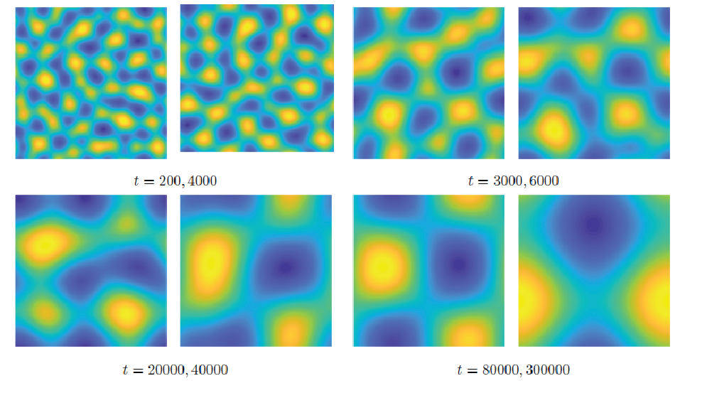
Refer to caption
Figure 2: (Color online.) Snapshots of the computed height function uu at the indicated times for the parameters L=12.8L=12.8, ε=0.02\varepsilon=0.02. The hills at early times are not as high as time at later times, and similarly with the valley. The average height/depth evolution with time could be seen in Figure 3.

The long time characteristics of the solution, especially the energy decay rate, average height growth rate, and the mound width growth rate, are of interest to surface physics community. The last two quantities can be easily measured experimentally. On the other hand, the discrete energy ENE_{N} is defined via (2.16); the space-continuous average height and average slope have been defined in (4.2), (4.3), and the analogous discrete versions are also available. Theoretically speaking, the lower bound for the energy decay rate is of the order of −ln⁡(t)-\ln(t), and the upper bounds for the average height and average slope/average length are of the order of t1/2t^{1/2}, t1/4t^{1/4}, respectively, as established for the no-slope-selection equation (1.3) in [29]. Figure 3 presents the semi-log plots for the energy versus time and log-log plots for the average height versus time, and average slope versus time, respectively, with the given physical parameter ε=0.02\varepsilon=0.02. The detailed scaling “exponents” are obtained using least squares fits of the computed data up to time t=400t=400. A clear observation of the −ln⁡(t)-\ln(t), t1/2t^{1/2} and t1/4t^{1/4} scaling laws can be made, with different coefficients dependent upon ε\varepsilon, or, equivalently, the domain size, LL.

Refer to caption  Refer to caption  Refer to caption

Figure 3: Left: Semi-log plot of the temporal evolution the energy ENE_{N} for ε=0.02\varepsilon=0.02. The energy decreases like −ln⁡(t)-\ln(t) until saturation. Middle: The log-log plot of the average height (or roughness) of uu, denoted as h⁡(t)h(t), which grows like t1/2t^{1/2}. Right: The log-log plot of the average width of uu, denoted m⁡(t)m(t), which grows like t1/4t^{1/4}. The dotted lines correspond to the minimum energy reached by the numerical simulation. The red lines represent the energy plot obtained by the simulations, while the straight lines are obtained by least squares approximations to the energy data. The least squares fit is only taken for the linear part of the calculated data, only up to about time t=400t=400. The fitted line for the energy has the form ae​ln⁡(t)+bea_{e}\ln(t)+b_{e}, with ae=−41.0983a_{e}=-41.0983, be=−148.6410b_{e}=-148.6410; the (blue) fitting line for the average height has the form ah​tbha_{h}t^{b_{h}}, with ah=0.4071a_{h}=0.4071, bh=0.5001b_{h}=0.5001, and the fitting line for the average width has the form am​tbma_{m}t^{b_{m}}, with am=4.1747a_{m}=4.1747, bm=0.2545b_{m}=0.2545.

Now we recall that a lower bound for the energy (1.1), assuming Ω=(0,L)2\Omega=(0,L)^{2}, which has been derived and polished in our earlier works [5, 7, 44]:

E⁡(ϕ)≥L22​(ln⁡(4​ε2​π2L2)−4​ε2​π2L2+1)=:γ.E(\phi)\geq\frac{L^{2}}{2}\left(\ln\left(\frac{4\varepsilon^{2}\pi^{2}}{L^{2}}\right)-\frac{4\varepsilon^{2}\pi^{2}}{L^{2}}+1\right)=:\gamma\ . (4.4)

Obviously, since the energy is bounded below it cannot keep decreasing at the rate −ln⁡(t)-\ln(t). This fact manifests itself in the calculated data as the rate of decrease of the energy, for example, begins to wildly deviate from the predicted −ln⁡(t)-\ln(t) curve. Sometimes the rate of decrease increases, and sometimes it slows as the systems “feels” the periodic boundary conditions. Interestedly, regardless of this later-time deviation from the accepted rates, the time at which the system saturates (i.e., the time when the energy abruptly and essentially stops decreasing) is roughly that predicted by extending the blue lines in Figure 3 to the predicted minimum energy (4.4).

Remark 4.1.

In this presented numerical simulation, the spatial resolution and time step sizes are taken as the same as the ones presented for the second order energy stable scheme [7]. Meanwhile, since a linear iteration algorithm has to be applied for the highly nonlinear numerical scheme in [7], the computational cost at each time step is about 3 to 5 times as the proposed 3rd order ETD-based one. For the long time simulation, both numerical schemes have produced similar evolutionary curves in terms of energy, standard deviation, and the mound width. A more detailed calculation shows that long time asymptotic growth rate of the standard deviation given by the third order numerical simulation is closer to t1/2t^{1/2} than that by the second order energy stable scheme: mr=0.5001m_{r}=0.5001, as recorded in Figure 3, while in [7] this exponent was found to be mr=0.5132m_{r}=0.5132. Similarly, the long time asymptotic growth rate of the mound width given by (2.24)-(2.25) is closer to t1/4t^{1/4} than that by the second order energy stable scheme in: bm=0.2545b_{m}=0.2545, as recorded in Figure 3, in comparison with mr=0.2607m_{r}=0.2607 reported in [7]. This gives more evidence that the third order scheme is able to produce more accurate long time numerical simulation results than the second order schemes, even if the computational cost is even less than the one given by [7], due to the linear iteration algorithm to implement the nonlinear numerical scheme.

Similar comparison has also been made between the second order ETD-related scheme and the proposed third order ETD-based scheme, given by (2.27) (outlined in [21]) and  (2.24)-(2.25), respectively: mr=0.5001m_{r}=0.5001, bm=0.2545b_{m}=0.2545 for the proposed third order scheme, in comparison with mr=0.510m_{r}=0.510, bm=0.258b_{m}=0.258, for E​T​D​M​s​2ETDMs2, as reported in [21]. This gives another evidence of robustness of the third order accurate numerical scheme for the NSS equation (1.3).

5 Concluding remarks

In this article, we propose and analyze a third order accurate ETD-based numerical scheme for the NSS equation (1.3) of the epitaxial thin film growth model, combined with Fourier pseudo-spectral spatial discretization. An exact integration of the linear part of the NSS equation is involved in the ETD-based scheme, followed by multi-step explicit approximation of the temporal integral of the nonlinear term. More importantly, a third order accurate Douglas-Dupont regularization term is added in the numerical scheme. In turn, a careful Fourier eigenvalue analysis leads to the energy stability in a modified version, and a uniform in time bound of the numerical energy becomes available. Furthermore, the optimal rate convergence analysis and error estimate are derived in details, with a decomposition of the numerical scheme into two stages. Error estimates are carried out in both stages, with extensive applications of linearized stability analysis in the second stage. To overcome the difficulties associated with many global operators involved in the algorithm, as well as their inverse operators, we have to perform careful eigenvalue estimates for these operators, as well as their composition. In addition, an aliasing error control technique has to be utilized in the ℓ∞​(0,T,Hh1)∩ℓ2​(0,T,Hh3)\ell^{\infty}(0,T,H_{h}^{1})\cap\ell^{2}(0,T;H_{h}^{3}) error estimate, combined with extensive scaling law arguments between Δ​t{\Delta t} and hh. This convergence estimate is the first such result for a third order accurate scheme for a gradient flow. Some numerical simulation results are presented to demonstrate the robustness of the numerical scheme and the third order convergence. In particular, the long time simulation results have revealed that, the power index for the surface roughness and the mound width growth for ε=0.02\varepsilon=0.02 (up to T=3×10⁵T=3\times 10^{5}), created by the proposed third order ETD-based numerical scheme, is more accurate than these created by certain second order accurate, energy stable schemes in the existing literature.

Acknowledgements

This work is supported in part by the Longshan Talent Project of SWUST 18LZX529 (K. Cheng), Hong Kong Research Council GRF grants 15300417 and 15325816, (Z. Qiao) and NSF DMS-1418689 (C. Wang).

Appendix A Proof of Lemma 2.4

First, we review the following estimate in Calculus.

Lemma A.1.

Suppose that f⁡(x)f(x) and g⁡(x)g(x) are continuous functions, f⁡(x)>0f(x)>0, g⁡(x)>0g(x)>0, and f⁡(x)g⁡(x)\frac{f(x)}{g(x)} is decreasing over (0,+∞)(0,+\infty). Define H⁡(x)=∫0xf⁡(t)​𝑑t∫0xg⁡(t)​𝑑tH(x)=\frac{\int_{0}^{x}f(t)dt}{\int_{0}^{x}g(t)dt}. Then H⁡(x)H(x) is decreasing over (0,+∞)(0,+\infty).

Proof.

Denote F⁡(x)=∫0xf⁡(t)​𝑑tF(x)=\int_{0}^{x}f(t)dt, G⁡(x)=∫0xg⁡(t)​𝑑tG(x)=\int_{0}^{x}g(t)dt, so that H⁡(x)=F⁡(x)G⁡(x)H(x)=\frac{F(x)}{G(x)}. For any 0<x1<x20<x_{1}<x_{2}, we make a comparison between H⁡(x1)H(x_{1}) and H⁡(x2)H(x_{2}).

We denote C1=f⁡(x1)g⁡(x1)C_{1}=\frac{f(x_{1})}{g(x_{1})}. By the decreasing property of f⁡(x)g⁡(x)\frac{f(x)}{g(x)}, we see that f⁡(x)g⁡(x)≥C1\frac{f(x)}{g(x)}\geq C_{1} for 0≤x≤x10\leq x\leq x_{1}, and f⁡(x)g⁡(x)≤C1\frac{f(x)}{g(x)}\leq C_{1} for x1≤x≤x2x_{1}\leq x\leq x_{2}. This in turn implies that

f⁡(x)≥C1​g​(x),for 0≤x≤x1,f⁡(x)≤C1​g​(x),for x1≤x≤x2.f(x)\geq C_{1}g(x),\,\,\,\mbox{for $0\leq x\leq x_{1}$},\quad f(x)\leq C_{1}g(x),\,\,\,\mbox{for $x_{1}\leq x\leq x_{2}$}. (A.1)

As a result, we get

∫0x1f⁡(t)​𝑑t≥C1​∫0x1g⁡(t)​𝑑t,∫x1x2f⁡(t)​𝑑t≤C1​∫x1x2g⁡(t)​𝑑t.\int_{0}^{x_{1}}f(t)dt\geq C_{1}\int_{0}^{x_{1}}g(t)dt,\quad\int_{x_{1}}^{x_{2}}f(t)dt\leq C_{1}\int_{x_{1}}^{x_{2}}g(t)dt. (A.2)

In turn, if we denote A1=∫0x1f⁡(t)​𝑑tA_{1}=\int_{0}^{x_{1}}f(t)dt, B1=∫0x1g⁡(t)​𝑑tB_{1}=\int_{0}^{x_{1}}g(t)dt, A2=∫x1x2f⁡(t)​𝑑tA_{2}=\int_{x_{1}}^{x_{2}}f(t)dt, B2=∫x1x2g⁡(t)​𝑑tB_{2}=\int_{x_{1}}^{x_{2}}g(t)dt, we have

A1B1≥C1≥A2B2.\frac{A_{1}}{B_{1}}\geq C_{1}\geq\frac{A_{2}}{B_{2}}. (A.3)

Then we arrive at

H⁡(x2)=∫0x2f⁡(t)​𝑑t∫0x2g⁡(t)​𝑑t=A1+A2B1+B2≤A1B1=H⁡(x1).H(x_{2})=\frac{\int_{0}^{x_{2}}f(t)dt}{\int_{0}^{x_{2}}g(t)dt}=\frac{A_{1}+A_{2}}{B_{1}+B_{2}}\leq\frac{A_{1}}{B_{1}}=H(x_{1}). (A.4)

This completes the proof for the decreasing property of H⁡(x)H(x). ∎

Next, we proceed into the proof of Lemma 2.4.

Proof.

The function g0​(x)g_{0}(x) could be represented as

g0​(x)=1−e−xx=∫0xe−t​𝑑t∫0x1​𝑑t.\displaystyle g_{0}(x)=\frac{1-{\rm e}^{-x}}{x}=\frac{\int_{0}^{x}{\rm e}^{-t}\,dt}{\int_{0}^{x}1\,dt}. (A.5)

On the other hand, e−x1=e−x\frac{{\rm e}^{-x}}{1}={\rm e}^{-x} is a decreasing function over (0,+∞)(0,+\infty). By Lemma A.1, we conclude that g0​(x)g_{0}(x) is decreasing.

Similarly, g1​(x)g_{1}(x) could be rewritten as

g1​(x)=x−(1−e−x)x2=∫0x(1−e−t)​𝑑t∫0x2​t​𝑑t.\displaystyle g_{1}(x)=\frac{x-(1-{\rm e}^{-x})}{x^{2}}=\frac{\int_{0}^{x}(1-{\rm e}^{-t})\,dt}{\int_{0}^{x}2t\,dt}. (A.6)

Since 1−e−x2​x=12​g0​(x)\frac{1-{\rm e}^{-x}}{2x}=\frac{1}{2}g_{0}(x) is a decreasing function over (0,+∞)(0,+\infty), an application of Lemma A.1 reveals that g1​(x)g_{1}(x) is also decreasing.

For g2​(x)g_{2}(x), we look at its rewritten form

g2​(x)=x2−2​(x−(1−e−x))x3=∫0x2​(t−(1−e−t))​𝑑t∫0x3​t2​𝑑t.\displaystyle g_{2}(x)=\frac{x^{2}-2(x-(1-{\rm e}^{-x}))}{x^{3}}=\frac{\int_{0}^{x}2(t-(1-{\rm e}^{-t}))\,dt}{\int_{0}^{x}3t^{2}\,dt}. (A.7)

Since 2​(x−(1−e−x))3​x2=23​g1​(x)\frac{2(x-(1-{\rm e}^{-x}))}{3x^{2}}=\frac{2}{3}g_{1}(x) is a decreasing function over (0,+∞)(0,+\infty), an application of Lemma A.1 reveals that g2​(x)g_{2}(x) is also decreasing. This finishes the proof of the first part of Lemma 2.4.

As a direct consequence of their decreasing property, we see that g0​(x)≤g0​(0)=1g_{0}(x)\leq g_{0}(0)=1, g1​(x)≤g1​(0)=12g_{1}(x)\leq g_{1}(0)=\frac{1}{2} and g2​(x)≤g2​(0)=13g_{2}(x)\leq g_{2}(0)=\frac{1}{3},     ∀x>0\forall x>0.

In turn, we observe that

g1​(x)g0​(x)≤g1​(0)g0​(2)=121−e−22=11−e−2,for x≤2,\displaystyle\frac{g_{1}(x)}{g_{0}(x)}\leq\frac{g_{1}(0)}{g_{0}(2)}=\frac{\frac{1}{2}}{\frac{1-{\rm e}^{-2}}{2}}=\frac{1}{1-{\rm e}^{-2}},\quad\mbox{for $x\leq 2$}, (A.8)
g1​(x)g0​(x)=1−1−e−xx1−e−x≤11−e−2,for x≥2.\displaystyle\frac{g_{1}(x)}{g_{0}(x)}=\frac{1-\frac{1-{\rm e}^{-x}}{x}}{1-{\rm e}^{-x}}\leq\frac{1}{1-{\rm e}^{-2}},\quad\mbox{for $x\geq 2$}. (A.9)

For the function g2​(x)g0​(x)\frac{g_{2}(x)}{g_{0}(x)}, we have

g2​(x)g0​(x)≤g2​(0)g0​(2)=131−e−22=23​(1−e−2),for x≤2,\displaystyle\frac{g_{2}(x)}{g_{0}(x)}\leq\frac{g_{2}(0)}{g_{0}(2)}=\frac{\frac{1}{3}}{\frac{1-{\rm e}^{-2}}{2}}=\frac{2}{3(1-{\rm e}^{-2})},\quad\mbox{for $x\leq 2$}, (A.10)
g2​(x)g0​(x)=1−2​1−1−e−xxx1−e−x≤11−e−2,for x≥2.\displaystyle\frac{g_{2}(x)}{g_{0}(x)}=\frac{1-2\frac{1-\frac{1-{\rm e}^{-x}}{x}}{x}}{1-{\rm e}^{-x}}\leq\frac{1}{1-{\rm e}^{-2}},\quad\mbox{for $x\geq 2$}. (A.11)

Therefore, the inequalities g1​(x)g0​(x)≤11−e−2\frac{g_{1}(x)}{g_{0}(x)}\leq\frac{1}{1-{\rm e}^{-2}}, g2​(x)g0​(x)≤11−e−2\frac{g_{2}(x)}{g_{0}(x)}\leq\frac{1}{1-{\rm e}^{-2}} are valid. This finishes the proof of Lemma 2.4. ∎

Appendix B Proof of Proposition 2.5

An application of Parseval equality to the discrete Fourier expansions for ff and 𝒢N(0)​f{\cal G}^{(0)}_{N}f, given by (2.35) and (2.39), respectively, leads to

‖f‖22=L2​∑k,ℓ=−KK|f^k,ℓ|2,‖𝒢N(0)​f‖22=L2​∑k,ℓ=−KKΔ​t​Λk,ℓ1−e−Δ​t​Λk,ℓ​|f^k,ℓ|2.\displaystyle\|f\|_{2}^{2}=L^{2}\sum_{k,\ell=-K}^{K}|\hat{f}_{k,\ell}|^{2},\quad\left\|{\cal G}^{(0)}_{N}f\right\|_{2}^{2}=L^{2}\sum_{k,\ell=-K}^{K}\frac{{\Delta t}\Lambda_{k,\ell}}{1-{\rm e}^{-{\Delta t}\Lambda_{k,\ell}}}|\hat{f}_{k,\ell}|^{2}. (B.1)

Meanwhile, the following observation is made:

Δ​t​Λk,ℓ1−e−Δ​t​Λk,ℓ=1g0​(Δ​t​Λk,ℓ).\displaystyle\frac{{\Delta t}\Lambda_{k,\ell}}{1-{\rm e}^{-{\Delta t}\Lambda_{k,\ell}}}=\frac{1}{g_{0}({\Delta t}\Lambda_{k,\ell})}. (B.2)

With an application of Lemma 2.4, we obtain

1=1g0​(0)≤1g0​(x)=x1−e−x≤1+x,∀x>0.\displaystyle 1=\frac{1}{g_{0}(0)}\leq\frac{1}{g_{0}(x)}=\frac{x}{1-{\rm e}^{-x}}\leq 1+x,\quad\forall x>0. (B.3)

This in turn implies that

1≤Δ​t​Λk,ℓ1−e−Δ​t​Λk,ℓ≤1+Δ​t​Λk,ℓ,for any k, ℓ.\displaystyle 1\leq\frac{{\Delta t}\Lambda_{k,\ell}}{1-{\rm e}^{-{\Delta t}\Lambda_{k,\ell}}}\leq 1+{\Delta t}\Lambda_{k,\ell},\quad\mbox{for any $k$, $\ell$}. (B.4)

Its combination with (B.1) reveals that

‖f‖22≤‖𝒢N(0)​f‖22≤L2​∑k,ℓ=−NN(1+Δ​t​Λk,ℓ)​|f^k,ℓ|2=‖f‖22+Δ​t​(ε2​‖ΔN​f‖22+κ​‖∇Nf‖22),\displaystyle\|f\|_{2}^{2}\leq\left\|{\cal G}^{(0)}_{N}f\right\|_{2}^{2}\leq L^{2}\sum_{k,\ell=-N}^{N}(1+{\Delta t}\Lambda_{k,\ell})|\hat{f}_{k,\ell}|^{2}=\|f\|_{2}^{2}+{\Delta t}(\varepsilon^{2}\|\Delta_{N}f\|_{2}^{2}+\kappa\|\nabla_{N}f\|_{2}^{2}), (B.5)

which in turn results in (2.42), by taking C1=1C_{1}=1.

The proof of the first inequality of (2.43) follows a similar form of Fourier analysis, combined with the following identity:

Δ​t​Λk,ℓ1−e−Δ​t​Λk,ℓ≥Δ​t​Λk,ℓ,∀k,ℓ.\displaystyle\frac{{\Delta t}\Lambda_{k,\ell}}{1-{\rm e}^{-{\Delta t}\Lambda_{k,\ell}}}\geq{\Delta t}\Lambda_{k,\ell},\quad\forall k,\ell. (B.6)

For the second inequality of (2.43), we begin with the following identities

(LN​f)i,j=∑k,ℓ=−KKΛk,ℓ​f^k,ℓ​e2​π​i​(k​xi+ℓ​yj)/L,\displaystyle(L_{N}f)_{i,j}=\sum_{k,\ell=-K}^{K}\Lambda_{k,\ell}\hat{f}_{k,\ell}{\rm e}^{2\pi i(kx_{i}+\ell y_{j})/L},
(−ΔN​e−LN​Δ​t​f)i,j=∑k,ℓ=−KK(−λk,ℓ)​e−Δ​t​Λk,ℓ​f^k,ℓ​e2​π​i​(k​xi+ℓ​yj)/L,\displaystyle(-\Delta_{N}{\rm e}^{-L_{N}{\Delta t}}f)_{i,j}=\sum_{k,\ell=-K}^{K}(-\lambda_{k,\ell}){\rm e}^{-{\Delta t}\Lambda_{k,\ell}}\hat{f}_{k,\ell}{\rm e}^{2\pi i(kx_{i}+\ell y_{j})/L},

so that

⟨LN​f,−ΔN​e−LN​Δ​t​f⟩=L2​∑k,ℓ=−KK(−λk,ℓ)​Λk,ℓ​e−Δ​t​Λk,ℓ​|f^k,ℓ|2≥0,\displaystyle\left\langle L_{N}f,-\Delta_{N}{\rm e}^{-L_{N}{\Delta t}}f\right\rangle=L^{2}\sum_{k,\ell=-K}^{K}(-\lambda_{k,\ell})\Lambda_{k,\ell}{\rm e}^{-{\Delta t}\Lambda_{k,\ell}}|\hat{f}_{k,\ell}|^{2}\geq 0, (B.7)

since −λk,ℓ≥0-\lambda_{k,\ell}\geq 0, Λk,ℓ≥0\Lambda_{k,\ell}\geq 0, and e−Δ​t​Λk,ℓ≥0{\rm e}^{-{\Delta t}\Lambda_{k,\ell}}\geq 0, for any k,ℓk,\ell.

The proof of (2.44) and (2.45) could be carried out in the same manner; the details are left to interested readers.

For the analysis of GN(1)​fG^{(1)}_{N}f, with its discrete Fourier expansion given by (2.37), an application of Parseval equality gives

‖f‖22=L2​∑k,ℓ=−KK|f^k,ℓ|2,‖GN(1)​f‖22=L2​∑k,ℓ=−KK(1−1−e−Δ​t​Λk,ℓΔ​t​Λk,ℓ1−e−Δ​t​Λk,ℓ)2​|f^k,ℓ|2.\displaystyle\|f\|_{2}^{2}=L^{2}\sum_{k,\ell=-K}^{K}|\hat{f}_{k,\ell}|^{2},\quad\left\|G^{(1)}_{N}f\right\|_{2}^{2}=L^{2}\sum_{k,\ell=-K}^{K}\Bigl(\frac{1-\frac{1-{\rm e}^{-{\Delta t}\Lambda_{k,\ell}}}{{\Delta t}\Lambda_{k,\ell}}}{1-{\rm e}^{-{\Delta t}\Lambda_{k,\ell}}}\Bigr)^{2}|\hat{f}_{k,\ell}|^{2}. (B.8)

On the other hand, the following observation is available:

1−1−e−Δ​t​Λk,ℓΔ​t​Λk,ℓ1−e−Δ​t​Λk,l=g1​(Δ​t​Λk,ℓ)g0​(Δ​t​Λk,ℓ)≤11−e−2,\displaystyle\frac{1-\frac{1-{\rm e}^{-{\Delta t}\Lambda_{k,\ell}}}{{\Delta t}\Lambda_{k,\ell}}}{1-{\rm e}^{-{\Delta t}\Lambda_{k,l}}}=\frac{g_{1}({\Delta t}\Lambda_{k,\ell})}{g_{0}({\Delta t}\Lambda_{k,\ell})}\leq\frac{1}{1-{\rm e}^{-2}}, (B.9)

with an application of Lemma 2.4 in the second step. Its substitution into (B.8) results in

‖f‖22=L2​∑k,ℓ=−KK|f^k,ℓ|2,‖GN(1)​f‖22≤(11−e−2)2​‖f‖22.\displaystyle\|f\|_{2}^{2}=L^{2}\sum_{k,\ell=-K}^{K}|\hat{f}_{k,\ell}|^{2},\quad\left\|G^{(1)}_{N}f\right\|_{2}^{2}\leq(\frac{1}{1-{\rm e}^{-2}})^{2}\|f\|_{2}^{2}. (B.10)

Then we have proved the first inequality of (2.46), with C4=11−e−2C_{4}=\frac{1}{1-{\rm e}^{-2}}.

The analysis of GN(2)​fG^{(2)}_{N}f could be carried out in the same manner, and the second inequality of (2.46) is with C5=11−e−2C_{5}=\frac{1}{1-{\rm e}^{-2}}. This finishes the proof of Proposition 2.5.

Appendix C Proof of Proposition 3.2

We begin with the following expansion:

∇N(fN​(Uk)−fN​(uk))=∇N∇N⋅(gN​(Uk)−gN​(uk)).\displaystyle\nabla_{N}\left(f_{N}(U^{k})-f_{N}(u^{k})\right)=\nabla_{N}\nabla_{N}\cdot\left(g_{N}(U^{k})-g_{N}(u^{k})\right). (C.1)

Meanwhile, we denote UNkU_{N}^{k}, uNku_{N}^{k} and eNke_{N}^{k} as the continuous extension of UkU^{k}, uku^{k} and eke^{k}, as the formula given by (2.17). We notice that gNg_{N} is defined in the sense of collocation way, at a point-wise level. Since gN​(Uk)−gN​(uk)g_{N}(U^{k})-g_{N}(u^{k}) is the grid point interpolation of g⁡(UNk)−g⁡(uNk)g(U_{N}^{k})-g(u_{N}^{k}), we apply (2.20) (in Lemma 2.2) to control the aliasing error. Subsequently, we arrive at

∥∇N∇N⋅(gN(Uk)−gN(uk))∥2=∥∇∇⋅PcN(g(UNk)−g(uNk))∥\displaystyle\|\nabla_{N}\nabla_{N}\cdot\left(g_{N}(U^{k})-g_{N}(u^{k})\right)\|_{2}=\|\nabla\nabla\cdot P_{c}^{N}\left(g(U_{N}^{k})-g(u_{N}^{k})\right)\| (C.2)
≤\displaystyle\leq C​‖PcN​(g⁡(UNk)−g⁡(uNk))‖H2≤C​‖g⁡(UNk)−g⁡(uNk)‖H2,\displaystyle C\|P_{c}^{N}\left(g(U_{N}^{k})-g(u_{N}^{k})\right)\|_{H^{2}}\leq C\|g(U_{N}^{k})-g(u_{N}^{k})\|_{H^{2}},

in which the fact that 2>d2=12>\frac{d}{2}=1 has been used. On the other hand, we have the following expansion for g⁡(UNk)−g⁡(uNk)g(U_{N}^{k})-g(u_{N}^{k}), in a similar form as (2.79):

g(UNk)−g(uNk)=∇eNk1+|∇uNk|2+∇(UNk+uNk)⋅∇eNk(1+|∇UNk|2)​(1+|∇uNk|2)∇UNk+κ∇eNk.\displaystyle g(U_{N}^{k})-g(u_{N}^{k})=\frac{\nabla e_{N}^{k}}{1+|\nabla u_{N}^{k}|^{2}}+\frac{\nabla(U_{N}^{k}+u_{N}^{k})\cdot\nabla e_{N}^{k}}{(1+|\nabla U_{N}^{k}|^{2})(1+|\nabla u_{N}^{k}|^{2})}\nabla U_{N}^{k}+\kappa\nabla e_{N}^{k}. (C.3)

A repeated application of Hölder inequality and Sobobev inequality leads to the following estimates:

∥∇eNk1+|∇uNk|2+κ∇eNk∥H2≤C(∥UNk∥H32+∥uNk∥H32)(∥∇eNk∥+∥ΔeNk∥+∥∇ΔeNk∥),\displaystyle\|\frac{\nabla e_{N}^{k}}{1+|\nabla u_{N}^{k}|^{2}}+\kappa\nabla e_{N}^{k}\|_{H^{2}}\leq C(\|U_{N}^{k}\|_{H^{3}}^{2}+\|u_{N}^{k}\|_{H^{3}}^{2})(\|\nabla e_{N}^{k}\|+\|\Delta e_{N}^{k}\|+\|\nabla\Delta e_{N}^{k}\|), (C.4)
∥∇(UNk+uNk)⋅∇eNk(1+|∇UNk|2)​(1+|∇uNk|2)∇UNk∥H2\displaystyle\|\frac{\nabla(U_{N}^{k}+u_{N}^{k})\cdot\nabla e_{N}^{k}}{(1+|\nabla U_{N}^{k}|^{2})(1+|\nabla u_{N}^{k}|^{2})}\nabla U_{N}^{k}\|_{H^{2}}
≤C(∥UNk∥H32+∥uNk∥H32)(∥∇eNk∥+∥ΔeNk∥+∥∇ΔeNk∥).\displaystyle\qquad\leq C(\|U_{N}^{k}\|_{H^{3}}^{2}+\|u_{N}^{k}\|_{H^{3}}^{2})(\|\nabla e_{N}^{k}\|+\|\Delta e_{N}^{k}\|+\|\nabla\Delta e_{N}^{k}\|). (C.5)

Meanwhile, with the a-priori assumption (3.12), we have

∥UNk∥H3≤C∗,∥uNk∥H3≤∥UNk∥H3+∥eNk∥H3≤∥UNk∥H3+C6∥∇ΔeNk∥≤C∗+C6:=C~1,\displaystyle\|U_{N}^{k}\|_{H^{3}}\leq C*,\quad\|u_{N}^{k}\|_{H^{3}}\leq\|U_{N}^{k}\|_{H^{3}}+\|e_{N}^{k}\|_{H^{3}}\leq\|U_{N}^{k}\|_{H^{3}}+C_{6}\|\nabla\Delta e_{N}^{k}\|\leq C^{*}+C_{6}:=\tilde{C}_{1}, (C.6)

in which C6C_{6} is a constant associated with elliptic regularity: ∥eNk∥H3≤C6∥∇ΔeNk∥\|e_{N}^{k}\|_{H^{3}}\leq C_{6}\|\nabla\Delta e_{N}^{k}\|, since ∫ΩeNk​𝑑𝐱=0\int_{\Omega}e_{N}^{k}\,d{\bf x}=0. Then we arrive at

‖∇N(fN​(Uk)−fN​(uk))‖2=‖∇N∇N⋅(gN​(Uk)−gN​(uk))‖2≤C​‖g⁡(UNk)−g⁡(uNk)‖H2\displaystyle\|\nabla_{N}\left(f_{N}(U^{k})-f_{N}(u^{k})\right)\|_{2}=\|\nabla_{N}\nabla_{N}\cdot\left(g_{N}(U^{k})-g_{N}(u^{k})\right)\|_{2}\leq C\|g(U_{N}^{k})-g(u_{N}^{k})\|_{H^{2}} (C.7)
≤\displaystyle\leq C(∥UNk∥H32+∥uNk∥H32)(∥∇eNk∥+∥ΔeNk∥+∥∇ΔeNk∥)\displaystyle C(\|U_{N}^{k}\|_{H^{3}}^{2}+\|u_{N}^{k}\|_{H^{3}}^{2})(\|\nabla e_{N}^{k}\|+\|\Delta e_{N}^{k}\|+\|\nabla\Delta e_{N}^{k}\|)
≤\displaystyle\leq C((C∗)2+C~12)C6∥∇ΔeNk∥≤C((C∗)2+C~12)C6∥∇NΔNek∥.\displaystyle C((C^{*})^{2}+\tilde{C}_{1}^{2})C_{6}\|\nabla\Delta e_{N}^{k}\|\leq C((C^{*})^{2}+\tilde{C}_{1}^{2})C_{6}\|\nabla_{N}\Delta_{N}e^{k}\|.

As a result, (3.13) has been established, by taking C0(2)=C⁡((C∗)2+C~12)​C6C_{0}^{(2)}=C((C^{*})^{2}+\tilde{C}_{1}^{2})C_{6}. This finishes the proof of Proposition 3.2.

References

  • [1] B. Benesova, C. Melcher, and E. Suli. An implicit midpoint spectral approximation of nonlocal Cahn-Hilliard equations. Numer. Math., 52:1466–1496, 2014.
  • [2] G. Beylkin, J.M. Keiser, and L. Vozovoi. A new class of time discretization schemes for the solution of nonlinear PDEs. J. Comput. Phys., 147:362–387, 1998.
  • [3] J. Boyd. Chebyshev and Fourier Spectral Methods. Dover, New York, NY, 2001.
  • [4] C. Canuto and A. Quarteroni. Approximation results for orthogonal polynomials in Sobolev spaces. Math. Comp., 38:67–86, 1982.
  • [5] W. Chen, S. Conde, C. Wang, X. Wang, and S.M. Wise. A linear energy stable scheme for a thin film model without slope selection. J. Sci. Comput., 52:546–562, 2012.
  • [6] W. Chen, W. Li, Z. Luo, C. Wang, and X. Wang. A stabilized second order ETD multistep method for thin film growth model without slope selection. SIAM J. Numer. Anal., 2018. Submitted and in review.
  • [7] W. Chen, C. Wang, X. Wang, and S.M. Wise. A linear iteration algorithm for energy stable second order scheme for a thin film model without slope selection. J. Sci. Comput., 59:574–601, 2014.
  • [8] W. Chen and Y. Wang. A mixed finite element method for thin film epitaxy. Numer. Math., 122:771–793, 2012.
  • [9] S.M. Cox and P.C. Matthews. Exponential time differencing for stiff systems. J. Comput. Phys., 176:430–455, 2002.
  • [10] W. E. Convergence of spectral methods for the Burgers’ equation. SIAM J. Numer. Anal., 29:1520–1541, 1992.
  • [11] W. E. Convergence of Fourier methods for Navier-Stokes equations. SIAM J. Numer. Anal., 30:650–674, 1993.
  • [12] G. Ehrlich and F. G. Hudda. Atomic view of surface diffusion: Tungsten on tungsten. J. Chem. Phys., 44:1036–1099, 1966.
  • [13] D.J. Eyre. Unconditionally gradient stable time marching the Cahn-Hilliard equation. MRS. Symp. Proc., 529:39, 1998.
  • [14] W. Feng, C. Wang, S.M. Wise, and Z. Zhang. A second-order energy stable Backward Differentiation Formula method for the epitaxial thin film equation with slope selection. Numer. Methods Partial Differ. Equ., 34(6):1975–2007, 2018.
  • [15] L. Golubović. Interfacial coarsening in epitaxial growth models without slope selection. Phys. Rev. Lett, 78:90–93, 1997.
  • [16] D. Gottlieb and S.A. Orszag. Numerical Analysis of Spectral Methods, Theory and Applications. SIAM, Philadelphia, PA, 1977.
  • [17] S. Gottlieb, F. Tone, C. Wang, X. Wang, and D. Wirosoetisno. Long time stability of a classical efficient scheme for two dimensional Navier-Stokes equations. SIAM J. Numer. Anal., 50:126–150, 2012.
  • [18] S. Gottlieb and C. Wang. Stability and convergence analysis of fully discrete Fourier collocation spectral method for 3-D viscous Burgers’ equation. J. Sci. Comput., 53:102–128, 2012.
  • [19] M. Hochbruck and A. Ostermann. Exponential integrators. Acta Numer., 19:209–286, 2010.
  • [20] M. Hochbruck and A. Ostermann. Exponential multistep methods of Adams-type. BIT Numer. Math., 51:889–908, 2011.
  • [21] L. Ju, X. Li, Z. Qiao, and H. Zhang. Energy stability and convergence of exponential time differencing schemes for the epitaxial growth model without slope selection. Math. Comp., 87:1859–1885, 2018.
  • [22] L. Ju, X. Liu, and W. Leng. Compact implicit integration factor methods for a family of semilinear fourth-order parabolic equations. Discrete Contin. Dyn. Syst. Ser. B, 19:1667–1687, 2014.
  • [23] L. Ju, J. Zhang, and Q. Du. Fast and accurate algorithms for simulating coarsening dynamics of Cahn-Hilliard equations. Comput. Mat. Sci., 108:272–282, 2015.
  • [24] L. Ju, J. Zhang, L. Zhu, and Q. Du. Fast explicit integration factor methods for semilinear parabolic equations. J. Sci. Comput., 62:431–455, 2015.
  • [25] R.V. Kohn. Energy-driven pattern formation. Proceedings of the International Congress of Mathematicians, M. Sanz-Sole, J. Soria, J.L. Varona, and J. Verdera, eds., European Mathematical Society Publishing House, Madrid, 1:359–384, 2007.
  • [26] R.V. Kohn and X. Yan. Upper bound on the coarsening rate for an epitaxial growth model. Comm. Pure Appl. Math., 56:1549–1564, 2003.
  • [27] B. Li. High-order surface relaxation versus the Ehrlich-Schwoebel effect. Nonlinearity, 19:2581–2603, 2006.
  • [28] B. Li and J. Liu. Thin film epitaxy with or without slope selection. Eur. J. Appl. Math., 14:713–743, 2003.
  • [29] B. Li and J. Liu. Epitaxial growth without slope selection: energetics, coarsening, and dynamic scaling. J. Nonlinear Sci., 14:429–451, 2004.
  • [30] D. Li and Z. Qiao. On second order semi-implicit fourier spectral methods for 2D Cahn-Hilliard equations. J. Sci. Comput., 70:301–341, 2017.
  • [31] D. Li and Z. Qiao. On the stabilization size of semi-implicit fourier-spectral methods for 3D Cahn-Hilliard equations. Commun. Math. Sci., 15:1489–1506, 2017.
  • [32] D. Li, Z. Qiao, and T. Tang. Characterizing the stabilization size for semi-implicit Fourier-spectral method to phase field equations. SIAM J. Numer. Anal., 54:1653–1681, 2016.
  • [33] D. Li, Z. Qiao, and T. Tang. Gradient bounds for a thin film epitaxy equation. J. Differential Equations, 262:1720–1746, 2017.
  • [34] W. Li, W. Chen, C. Wang, Y. Yan, and R. He. A second order energy stable linear scheme for a thin film model without slope selection. J. Sci. Comput., 76(3):1905–1937, 2018.
  • [35] X. Li, Z. Qiao, and H. Zhang. Convergence of a fast explicit operator splitting method for the epitaxial growth model with slope selection. SIAM J. Numer. Anal., 55:265–285, 2017.
  • [36] D. Moldovan and L. Golubovic. Interfacial coarsening dynamics in epitaxial growth with slope selection. Phys. Rev. E, 61(6):6190, 2000.
  • [37] Z. Qiao, Z. Sun, and Z. Zhang. The stability and convergence of two linearized finite difference schemes for the nonlinear epitaxial growth model. Numer. Methods Partial Differ. Equ., 28:1893–1915, 2012.
  • [38] Z. Qiao, Z. Sun, and Z. Zhang. Stability and convergence of second-order schemes for the nonlinear epitaxial growth model without slope selection. Math. Comp., 84:653–674, 2015.
  • [39] Z. Qiao, C. Wang, S.M. Wise, and Z. Zhang. Error analysis of a finite difference scheme for the epitaxial thin film growth model with slope selection with an improved convergence constant. Int. J. Numer. Anal. Model., 14:283–305, 2017.
  • [40] Z. Qiao, Z. Zhang, and T. Tang. An adaptive time-stepping strategy for the molecular beam epitaxy models. SIAM J. Sci. Comput., 33:1395–1414, 2012.
  • [41] R. L. Schwoebel. Step motion on crystal surfaces: II. J. Appl. Phys., 40:614–618, 1969.
  • [42] J. Shen, C. Wang, X. Wang, and S.M. Wise. Second-order convex splitting schemes for gradient flows with Ehrlich-Schwoebel type energy: Application to thin film epitaxy. SIAM J. Numer. Anal., 50:105–125, 2012.
  • [43] H. Song and C.-W. Shu. Unconditional energy stability analysis of a second order implicit-explicit local discontinuous Galerkin method for the Cahn-Hilliard equation. J. Sci. Comput., 73:1178–1203, 2017.
  • [44] C. Wang, X. Wang, and S.M. Wise. Unconditionally stable schemes for equations of thin film epitaxy. Discrete Contin. Dyn. Syst., 28:405–423, 2010.
  • [45] X. Wang, L. Ju, and Q. Du. Efficient and stable exponential time differencing Runge-Kutta methods for phase field elastic bending energy models. J. Comput. Phys., 316:21–38, 2016.
  • [46] C. Xu and T. Tang. Stability analysis of large time-stepping methods for epitaxial growth models. SIAM J. Numer. Anal., 44(4):1759–1779, 2006.
  • [47] X. Yang, J. Zhao, and Q. Wang. Numerical approximations for the molecular beam epitaxial growth model based on the invariant energy quadratization method. J. Comput. Phys., 333:104–127, 2017.
  • [48] L. Zhu, L. Ju, and W. Zhao. Fast high-order compact exponential time differencing Runge-Kutta methods for second-order semilinear parabolic equations. J. Sci. Comput., 67:1043–1065, 2016.