Smoothing -gradients in iterative regularization
Abstract.
Connected with the rise of interest in inverse problems is the development and analysis of regularization methods, which are a necessity due to the ill-posedness of inverse problems. Tikhonov-type regularization methods are very popular in this regard. However, its direct implementation for large-scale linear or non-linear problems is a non-trivial task. In such scenarios, iterative regularization methods usually serve as a better alternative. In this paper we propose a new iterative regularization method which uses descent directions, different from the usual gradient direction, that enable a more smoother and effective recovery than the later. This is achieved by transforming the original noisy gradient, via a smoothing operator, to a smoother gradient, which is more robust to the noise present in the data. It is also shown that this technique is very beneficial when dealing with data having large noise level. To illustrate the computational efficiency of this method we apply it to numerically solve some classical integral inverse problems, including image deblurring and tomography problems, and compare the results with certain standard regularization methods, such as Tikhonov, TV, CGLS, etc.
Key words and phrases:
Inverse problems, Iterative regularization, Variational minimization, Ill-posed problems, Integral equations, Tikhonov regularization.1991 Mathematics Subject Classification
Primary 65R30, 65R32; Secondary 65R20, 65K101. Introduction
1.1. Inverse Problems and Regularization:
An inverse problem in general is a problem where the output (effext) is known but the input (source) is not, in contrast to a direct problem where we deduce the effect from the source. Mathematically, an inverse problem is often expressed as the problem of finding/estimating a , given , which satisfies the following operator equation:
| (1.1) |
where is also a known operator describing the underlying physical process, the domain and range of varies depending on the problem. Typically, the solution of (1.1) is approximated by the solution of a least-square problem, i.e.
| (1.2) |
However, inverse problems are usually ill-posed, in the sense of violating Hadamard’s third condition: “Continuous dependence of the data”, i.e., even for a slightly perturbed data , such that (usually small), the inverse recovery becomes unstable, (very large), due to the unboundedness of the (pseudo-) inverse operator and the noise present in the data. To counter such instabilities or the ill-posedness of inverse problems, regularization methods have to be employed. In the last few decades, several regularization methods have been established for linear as well as nonlinear inverse problems. Broadly, there exist two kinds of regularization approaches:
1.2. Tikhonov-type regularization:
Tikhonov-type regularization methods are probably the most well known regularization techniques for solving linear as well as nonlinear inverse problems (see [1, 2, 3, 4, 5]), where (instead of minimizing the simple least-square problem (1.2)) one recovers a regularized solution by minimizing a (constrained or) penalized functional
| (1.3) |
(for some and ) where is a called the regularization parameter, is the error norm, is an initial guess and is a regularization operator, with the null spaces of and intersecting trivially. The choice of an appropriate parameter value () is crucial here, as it balances between the data fitting term and the regularization term . If is too small then minimizing (1.3) over-fits the noisy data (thus, leading to a noisy recovery or, statistically speaking, a high-variance recovery), where as, if is too big then it under-fits the data (thus, leading to an over-smooth recovery, or statistically, a high-bias recovery). Choosing an appropriate is not a trivial task, especially when dealing with large-scale problems, and typically one has to compute the solutions for many different values before choosing an appropriate .
1.3. (Semi-) Iterative regularization:
Contrary to the above approach, in a (semi-) iterative regularization method one recovers a regularized solution of (1.1) by simply stopping the minimization process of the least-square problem (1.2) at an appropriate (early) instance. That is, starting from an initial guess , one updates the recovered solution () in a direction () such that the recovered solution () is better than the previous, meaning , and stops the iteration after certain number of steps (i.e., , for some appropriate , usually depending on the noise level ). Mathematically,
| (1.4) |
where is the m-th step-length and the descent direction is usually the negative gradient of the least-square functional , i.e., . When the step-size is fixed () for all , it’s known as Landweber iterations (also known as Richardson iterations) and has been intensively investigated in the literature (see, [6, 7, 1, 2, 8, 9]). The main drawback of Landweber iterations is its slow performance, i.e., it takes a large number of iterations to obtain the optimal convergence rates. To circumvent this drawback many extensions (known as polynomial or accelerated Landweber methods) have been proposed and studied in the framework of regularization (for an overview, see [8, 9, 10, 11]). Such iterative methods are typically known as semi-iterative methods, since when dealing with a noisy data () one encounters a semi-convergent nature of the recovery process. The advantage of these extended semi-iterative methods over the simple Landweber iteration is that, while Landweber iteration (1.4) uses only the last iterate to construct the new approximate , in a semi-iterative method one make use of the last few iterates (if not all),
| (1.5) | |||
where is the descent direction (usually ). Note that, belongs to the Krylov-subspace , which is defined as
| (1.6) |
Hence, these methods are also called as Krylov-subspace methods. Even further acceleration is possible by adapting a conjugate-gradient type method (see [12]), where in (1.5) depend on data (making it a non-linear method).
1.4. A new iterative regularization method:
First note that, starting from the simple Landweber iterations (1.4), all the generalizations and extensions (1.5) developed in the iterative regularization literature is focused only on improving the speed of the convergence of the descent process. In this paper, we discuss a new iterative regularization method that not only improves the descent rate but also improves the smoothness of the recovery, especially when dealing with data having large noise level, and hence, leads to a much effective and efficient recovery. Note that, in all of the aforementioned iterative methods there is a direct influence of the noisy data in the descent direction, i.e., . Therefore, when the noise level is large then the recovered solution (though regularized) sometimes still possesses some of the noisy characteristics arising from , especially when is large and does not compensate its noisy influence, see Example 6.1. Here, we present a technique to pre-condition the gradient, using a smoothing operator, so that it significantly reduces the noisy influence of , and thus, enhance the smoothness and accuracy of the recovery. First we observe that, a typical real-life data is usually contaminated by additive noise of zero mean, i.e., , where is a random variable such that and . Also, notice that integrating the noisy data smooths out the noise present in the data, for example, see Figure 1(a) ( vs. , with a relative error ) vs. Figure 1(b) ( vs. , with ). This provides a heuristic motivation to incorporate the integrated data (in a regularized manner) during the minimization process to improve the smoothness of the recovery, the theoretical justifications and implementations are demonstrated in the later sections.


We briefly outline our new method here. Let’s assume the operator as a linear bounded injective11 1 for simplicity, we work in an unique solution scenario. For a non-injective one can look for the minimal norm solution or the generalized solution (pseudo-inverse solution). operator, where and is a known function defined on , a bounded set. Here and are Hilbert spaces, that we consider to be subsets of . Then an approximate solution of problem (1.1) is attained in an iterative fashion using the following descent direction
| (1.7) |
where the integral operator is defined as follows: for any , is the solution of the following boundary value problem
| (1.8) | |||
Similar to (1.2), we show that the Variational formulation, related to the gradient defined in (1.7), corresponds to the minimization of the following functional
| (1.9) |
where and , and the operator is as defined above in (1.8). Equivalently,
| (1.10) |
For the exact , the first term in equation (1.9) is minimized by the solution () of the inverse problem and in §3 we prove that the second term also has the same minimizer, i.e., the solution of (1.1) is the minimizer of the functional .
Remark 1.1.
One may suspect that using an additional integral operator (in the second term of (1.9)) might increase the ill-posedness of the problem. But, as we are not using the noisy data directly for that term, rather a smoothed version of it (i.e., ) such that , the ill-posedness of the problem is not deteriorated. In addition, the first part (involving the original operator and data ) together with a stopping criterion depending on also influence the recovery of a regularized solution (). In fact, we will show that with proper integration techniques and using both the terms one can attain even lower relative errors during the descent process than using only the first term and can also significantly reduce the semi-convergent nature of the relative errors, see Figures 3(b), 4(g) and 4(h).
Remark 1.2.
Note that, since (in practice) we only deal with discrete data sets, to solve an inverse problem in higher dimension () one can convert the n-dimensional array to an one dimensional vector and apply the techniques developed for one dimensional problems. Hence, in this paper we develop the theories only for 1-dimensional problems and apply it solve n-dimensional problems (), like image deblurring and tomography, see Examples 6.2 and 6.3.
Here, we follow an improved descent algorithm for the inverse recovery of , where we first start with the normal -gradient of and then upgrade it to various other gradients, including the -gradient, to enhance the descent rate and efficiency of the recovery. Using an appropriate gradient is very crucial in the optimization process as it helps to retrieve the features of more accurately, for example, the -gradient not only smooths the noisy -gradient but also helps in pre-conditioning certain desired boundary effects, depending on some prior information of the boundary data, (see Example 6.1), details discussed in §4.
In §3 we prove the convexity (and some other properties) of the functional . In §4 we provide a descent algorithm to minimize the functional by using different gradients (or descent directions) depending on the scenarios, which is crucial for the minimization process. The convergence of the sequence of functions constructed during the descent process to a regularized solution and its stability are discussed in §5. To validate the numerical viability of the developed theory we perform numerous computational experiments, provided in §6, on some classical inverse problems, like Fredholm type and Volterra type integral equations, and compare our results with the results obtained using certain standard regularization methods, like Tikhonov-type methods, CGLS, LSQR, TV and more, see Tables 1 and 2.
2. Notations and Preliminaries
We adopt the following notations that are used throughout the paper. All functions are real-valued defined on a bounded closed domain . For , := denotes the usual Banach space of integrable functions on and the space contains the essentially bounded measurable functions. Likewise the Sobolev space contains all the functions for which and the space . The spaces and are Hilbert spaces with inner-products denoted as and , respectively.
Remark 2.1.
Note that, integrating the data () twice results in . This is particularly very significant in the sense that we are able to upgrade the smoothness of the working data or information space from to and hence improve the smoothness of the recovery.
Remark 2.2.
Also, note that the negative Laplacian operator is a positive operator in on . And using the positiveness of the operator on we can have a bound for as
| (2.1) |
where is the first (smallest) eigenvalue of the positive operator . Inequality (2.1) also implies, for a sequence of functions , if and only if , details in §5.
3. Convexity of the functional G
Now let us define functionals and corresponding to the first and the second terms of the functional as follows
| (3.1) | ||||
| (3.2) |
We first analyze the functional and then extend it to the functional .
Theorem 3.1.
- (1)
An equivalent form of , for any , is
(3.3) - (2)
For any two , we have
(3.4) - (3)
The first Gâteaux differential, at , for is given by
(3.5) where . The -gradient of , at , is given by
(3.6) where the is the adjoint of the operator .
- (4)
The second Gâteaux differential, at any , of is given by
(3.7) where and on . Hence for any , is a positive definite quadratic form.
Thus is a strictly convex22 2 the strict convexity follows if the operator is injective, otherwise, is a convex functional. functional and has a unique global minimum which is attained at .
First we state an ancillary result related to .
Lemma 3.2.
For fixed , we have
| (3.8) |
in .
Proof.
Subtracting the following equations
we have
| (3.9) |
and using we get, via integration by parts,
Now using the positiveness of the negative laplacian, we have , where is the smallest eigenvalue of , and thus
where the last line is obtained using the Cauchy-Schwarz inequality. Hence,
in , since the operator is bounded and are fixed, which implies the right hand side is of .
∎
Proof of Theorem 3.1
The proof of first two properties (i) and (ii) are straight forward via integration by parts and using the fact that . In order to prove (3) and (4), we use Lemma 3.2.
- (3)
The Gâteaux derivative of the functional at in the direction of , where , is given by
(3.10) Now for a fixed , we have using 3.9,
Using Lemma 3.2, one obtains the Gâteaux derivative of at in the direction of as
Note that for all , where is the adjoint of the operator , as . Hence, by Riesz representation theorem, the -gradient of the functional at is given by
- (4)
Finally, the second Gâteaux derivative for the functional at is given by
(3.11) Again for a fixed , we have using (3.9)
Hence from (3.11) and letting we get
Here we can see the strict convexity of the functional , as for any , we have
where and (from (3.9)). As is a positive operator on , is the trivial solution iff iff (T being strictly convex). Thus is a positive definite form for any . ∎
Now one can similarly prove the above properties for functional and extend it for functional as well, which is as follows:
Theorem 3.3.
- (1)
For any two , we have
(3.12) - (2)
The first Gâteaux differential, at , for G is given by
(3.13) where . The -gradient of , at , is given by
(3.14) where is the adjoint of the operator .
- (3)
The second Gâteaux differential, at any , of G is given by
(3.15) where . Hence for any , is a positive definite quadratic form.
4. The Descent Algorithm for G
In this section we discuss the problem of minimizing the functional , via a descent method. One can guess a descent direction by looking at the truncated Taylor expansion of the functional , which is
| (4.1) |
for any , , and sufficiently small . Thus is minimized at if the direction is chosen such that for an appropriate .
The followings are some descent directions that can make .
4.1. The -Gradient.
First, notice from Theorem 3.3 that at a given point
| (4.2) |
so if we choose the direction at , then . Though this gradient works well in most situations, there are certain issues associated with it during the descent process. From a theoretical point of view, if for some at every step of the descent process then will be invariant during the descent process and if then it will lead to severe decay or fluctuation near the point , for details see [13]. For example, if is a Volterra operator then the -gradient at any is always zero at the end point , since , which implies that at the end point the recovery will be invariant during the descent process, see Example 6.1.
4.2. The -Gradient.
One can circumvent the above problem by opting for the Sobolev or Neuberger gradient, , instead. It is the solution of the following boundary value problem
| (4.3) |
This provides us a gradient , at any , with considerably more flexibility at the boundary points . In particular one has
- (1)
Dirichlet Neuberger gradient : and .
- (2)
Neumann Neuberger gradient : and .
- (3)
Robin or Mixed Neuberger gradient : and or and .
In addition to the flexibility at the end points, it also enables the new gradient to be a preconditioned (smoothed) version of , as , and hence gives a superior convergence in the steepest descent algorithms when recovering a smooth function, see Example 6.1. One can also exploit the flexibility of the gradient at the end points according to some prior information of at the end points. For example, if prior knowledge of and are known, then one can define as the straight line joining them and use the Dirichlet Neubeger gradient for the descent. Thus the boundary data is preserved in each of the evolving ’s during the descent process which leads to a more efficient and faster descent than compared to the normal -gradient. Even when is unknown, one can use the Neumann Neuberger gradient that allows free movements at the boundary points rather than gluing to some fixed values, see Example 6.1.
4.3. The Conjugate Gradient.
Now, one can make use of both the gradients by taking computing the standard Polak-Ribiére conjugate gradient scheme (see [14]) to further boost the descent rate, approximately by a factor of 2. Specifically, the initial search direction at is . At one can use an exact or inexact line search routine to minimize in the direction of resulting in . Then and where
| (4.4) |
4.4. The line search method for the functional G
At any given the functional is minimzed in the gradient direction via the single variable function and using a line search minimization, where . To bracket the minimum the initial step size is chosen by solving the quadratic approximation of the function (see [13]), which is given by
| (4.5) |
and since the expressions for and are known, one can easily compute .
Hence during the descent process, starting from an initial guess , we obtain a sequence of -functions for which the sequence is strictly decreasing. In the next section, we discuss the convergence of to and the stability of the recovery.
5. Convergence and Regularization
Exact data: We first prove that the sequence of functions constructed during the descent process converges to the exact solution in the absence of any noise and then proves the stability of the process in the presence of noise.
5.1. Convergence
Note that, for the sequence produced by the steepest descent algorithm (described in Section 4) we have , as the functional is non-negative and strictly convex (with the global minimizer , such that G() = 0) and . The following theorems describe the convergence of the sequence {} to in .
We first prove the convergence result for and then extend it for .
Theorem 5.1.
Suppose that is any sequence of -functions such that the sequence tends to zero. Then , and the corresponding sequence , converge in to and , respectively, and the sequence converges to in .
Proof.
First note that, using the positivity of in on , we have
| (5.1) |
where is the smallest eigenvalue of . This immediately gives in . Now one can easily see the weak convergence for the sequences and in to and , respectively. Since in , this implies in . Thus, for any in the range of we have
| (5.2) | ||||
implying in , and since the range of is dense in for the linear, bounded and injective , we have in .
To see the strong convergence, we first express the functional in terms of an associated operator, i.e. , for some operator such that . One can show that, from (1.10), the function can be expressed as, for any and ,
| (5.3) |
and hence, the operator can be expressed as
| (5.4) |
From (5.4) one can see that the operator is also linear and bounded in , and thus, from the convergence theories developed for Landweber iterations or steepest descent methods, see [1, 15], the sequences and also converge to and , respectively, in . ∎
Similarly, one can extend the convergence results for functional as
Theorem 5.2.
Suppose that is any sequence of -functions such that the sequence tends to zero. Then , and the corresponding sequence , converge in to and , respectively, and converges to in .
5.2. Regularization (through appropriate early stopping)
As explained earlier, when solving an ill-posed problem with noisy data, one can not recover a regularized solution by simply minimizing the associated functional ( in (1.2) or in (3.1)) completely. Here, the recovery error follows a semi-convergent nature, i.e., in the initial iterations the sequence converges towards the true solution () but upon further iterations diverges away from , due to the noise and ill-posedness of the problem. Equivalently, during the initial stage for (for some appropriate ), but upon further iterations (or ), as . Hence such methods are also called as semi-iterative methods and terminating the minimization process at an appropriate early iteration leads to a regularized solution, i.e., the iteration index () serves as a regularization parameter, for details see [1, 15].
Here we show that the semi-convergent nature is also shown by the functional when recovering the true (or original) solution but using a noisy data . First we see that for an exact (or equivalently, an exact ) and the functional () constructed based on it, we have the true solution satisfying . However, for a given noisy , with , and the functional () based on it we will have , see Theorem 5.3. So if we construct a sequence of functions , using the descent algorithm and based on the noisy data , such that then (from Theorem 5.1 or 5.2) we will have , where is the recovered noisy solution satisfying . This implies initially and then upon further iterations diverges away from and approaches , such that . This typical behavior of any ill-posed problem is managed, as stated above, by stopping the descent process at an appropriate iteration such that but close to zero, this gives us a regularized solution such that .
Following a similar argument as in (2.1) we have a lower bound for as
Theorem 5.3.
Let and be the functionals defined corresponding to the given data and (or ) and, denote their respective minimizers (i.e., and ), then we have the following lower bound for
| (5.5) |
where is the smallest eigenvalue of the positive operator on , and vice-versa for .
5.3. Stopping criterion I
When the error norm is known then Morozov’s discrepancy principle, [5], can serve as a stopping criterion for the descent process, i.e., terminate the iteration when
| (5.8) |
for an appropriate 33 3 In our experiments, we used the termination condition: .. For the convergence and stability of the process see [7].
6. Numerical Results
We follow the following (pseudo-) Algorithm 1 and perform inverse recoveries on some standard integral type equations. A MATLAB code was written to test the numerical viability of the method and the results obtained are then compared with certain standard regularization methods, see Table 1 and Table 2.
while do
• • , with Neumann B.C., if • Conjugate gradients (), as defined in §(4.3), for faster descent rate Define: := - and :=
Find the optimal , as defined in (4.5)
if then
;
while do
;
6.1. Fredholm Integral Equation of the First Kind
A Fredholm integral equation of the first kind is an integral operator equation that depends on a kernel function and is given by
| (6.1) |
Such integral operator equations are classical inverse problems and can be quite ill-posed. The operator equation (6.1) is discretized using either Galerkin or Nystrm methods to yield the following linear discrete ill-posed problem
| (6.2) |
where the matrix is the discretized representation of the operator and the vectors , the are the discretized source and effect functions. MATLAB functions in [16, 17, 18] determine the discretizations , the scaled discrete approximations of and . To test the stability of the method, a Gaussian (zero-mean) error vector is added to to get a perturbed vector , such that (the relative error norm) is around , unless otherwise stated. In particular, when using discrepancy principle to terminate the descent process we assume to be known.
6.2. Numerical Differentiation
In the first example we study the problem of numerical differentiation (of noisy data), which is also governed by an integral equation (also known as a Volterra equation) of the following form
| (6.3) |
for , and comparing (6.3) to (6.1), the kernel function can be considered as , where is the standard characteristic function, for details see [13]. Now, for some given discrete noisy data values , we construct a discrete set of values for the function , as defined in (1.10). Note that, when using the formula (1.10) to construct or , the values of and depend on the choice of the value of the integration mesh-size , because of the discretization of the integral, where for any integrable function ,
| (6.4) |
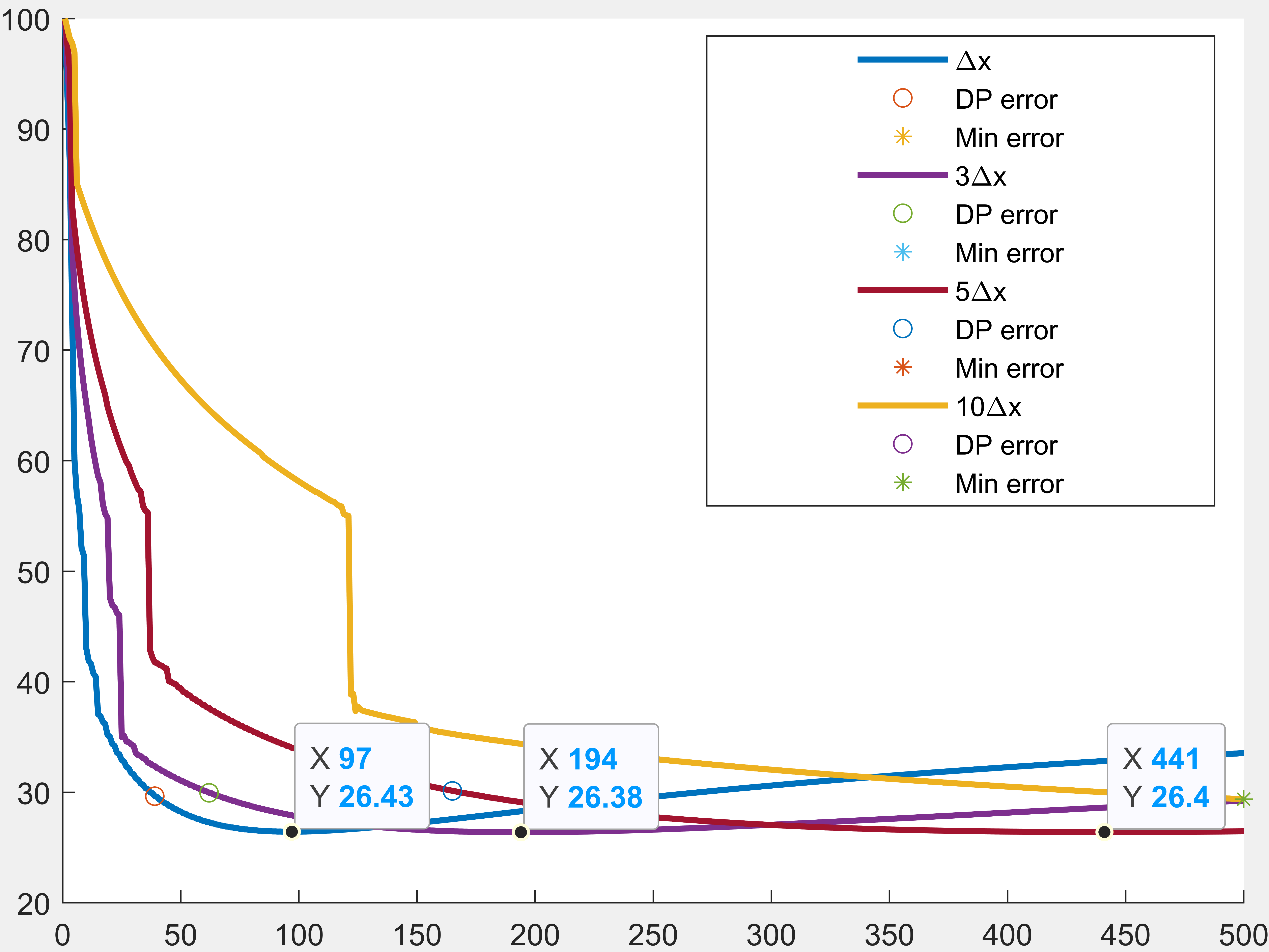
Hence, in the following examples we show that increasing the values leads to smoother solutions as well as saturating the relative errors in the recovery. Since the kernel function is a simple step-function, which is not smooth, one can notice (see Figure 2) that the recovered solution obtained using the discrepancy principle, though regularized, is also not smooth. However, with increasing values the smoothness of the recovery increases, see Figure 3(a). Also, note that here (as explained in §4.1) using or - conjugate gradient wouldn’t be a good choice if , as (since ), which leads to a sharp decay at the end point ‘b’, see Figure 2(b) and Table 1. In such scenarios, either Neumann or - conjugate gradient will be very effective.
Example 6.1.
We contaminate two functions and on with Uniform noise, to produce noisy and with a relative noise level of 10%. We collected evenly spread 200 of those noisy data points, which corresponds to a grid-size of 0.01. Note that, since on , we have . Now we compute the numerical regularized-derivatives from these noisy ’s data points and compare it with the true derivatives ’s. Figure 2 shows the comparison of the recoveries obtained using Tikhonov regularization and our method with the - conjugate gradient and the - conjugate gradient, with the relative errors in Table 1. Note that, when computing (where ) the use of Neumann - conjugate gradient leads to a much better and smoother recovery, because of the flexibility at the boundary point and (leading to a smoother gradient).
In the above computations we used the integration mesh-size for constructing and . Then we repeat the experiment with the same number of noisy data points but with different values for the integration. Note that, here represents the mesh-size for the integral to get or values and is not connected to the original grid-size of the problem (which determines the number of data points). Figure 3(a) shows the increase in the smoothness level with the increase in the values and Figure 3(b) shows the saturating effect shown by increasing values. In fact, increasing values not only saturates the recovery errors during the descent process but also lowers the minimum error of the recovery (though we cannot obtain that solution directly from the discrepancy principle).


| Stopping strategy: Morozov’s discrepancy principle, see (5.8) | ||||||
| Methods | ||||||
| Tik () | 0.1179 | 0.2748 | ||||
| Tik () | 0.1822 | 0.2205 | ||||
| TSVD | 0.0695 | 0.2734 | ||||
| TTLS | 0.4544 | 0.3521 | ||||
| CGLS | 0.0814 | 0.2543 | ||||
| LSQRB | 0.0814 | 0.2543 | ||||
| -method | 0.1734 | 0.2651 | ||||
| G () | 0.0803 | 0.0720 | 0.0661 | 0.2574 | 0.2691 | 0.2921 |
| G () | 0.1608 | 0.1907 | 0.1861 | 0.1474 | 0.2237 | 0.2218 |
6.3. Imaging Problems
In this subsection we deal with higher dimensional inverse problems. Considering an image as a matrix leads to a 2-dimensional problem. However, we can transform a two dimensional -matrix to an one dimensional vector of length by simply stacking either the columns or rows over each other and hence, converting the 2-dimensional problem to a 1-dimensional problem. Now, since the integral limits can be arbitrary we assign the limits based on grid or mesh size, i.e., assuming and some value for we have . Here, since the transformed 1D vector corresponding to an image is highly discontinuous and non-smooth, having a large value leads to over-smooth the solution. Hence, we start with the initial choice and show that with conservative increments one can attain a similar saturation of the relative errors as shown in Figure 3(b). We used as the descent direction during the recovery process and the dependence of the relative errors on the integration mesh-size () is projected in Figure 4.
Example 6.2.
Image deblurring
In this example we apply our regularization technique to deblurr a noisy blurred image. The mechanism behind blurring an image also results in a Fredholm integral equation of first kind (6.1), with kernel being a Gaussian spread function, i.e., , where determines the spread and the ill-posedness of the problem (ill-posedness increases with the increase in the value, here we considered ). A true test image (), see Figure 4(a), is first blurred and then contaminated with Gaussian noise ( 10% relative error) to get a blurred noisy image (), see Figure 4(c). Again, the discretized matrix and the vectors , in (where ) are generated using the routine, , from [16, 18]. In this problem we performed a constraint minimization44
4
i.e., we project the negative values to zero., , during the recovery process, since the pixel values are non-negative, and used the gradient as the descent direction. Figure 4(e) shows the recovered image (using functional ) and Table 2 shows an error comparison between our recovery and the recoveries obtained by using some of the standard iterative regularization methods such as Least Squares minimization with (i) -norm (IRell1), (ii) (heuristic) total variation penalization (IRhtv), (iii) Conjugate Gradient (CGLS), (iv) FISTA for constrained LS (IRfista), (v) modified residual norm steepest descent (IRmrnsd), (vi) enriched CGLS (IRenrich), (vii) -norm penalization term (IRirn), (viii) hybrid FGMRES for enforcing -norm penalization (IRhybrid_fgmres), (ix) hybrid GMRES for square systems (IRhybrid_gmres), (x) hybrid LSQR (IRhybrid_lsqr), (xi) restarted Krylov subspace method (IRrestart), where the routines for the above mentioned methods are taken from [17], with the non-negative constraint (i.e., ‘nonnegativity’,‘on’) and the stopping rule as the discrepancy principle (‘stoprule’,‘DP’).


Example 6.3.
[Tomography test problem]
In this example we considered the tomography test problem from [18], where the matrix and the vectors , (where ) are generated using the routine, , defined in [17]. The true image is shown in Figure 4(b) and the noisy image ( 10% relative noise) for vector is shown in Figure 4(d). Here, we again performed a constrained minimization () during the descent process, as in Example 6.2. The recovered image is shown in Figure 4(f) and Table 2 shows an error comparison between our method and some of the standard iterative regularization methods mentioned in Example 6.2.
| Relative errors in the recoveries using different regularization methods. | ||||
| Deblurring | Tomography | |||
| Methods | Relative error | Sparsity (# 0s) | Relative error | Sparsity (# 0s) |
| IRell1 | 0.3126 | 0 | ||
| IRhtv | 0.3361 | 5732 | 0.5404 | 225 |
| IRcgls | 0.2353 | 0 | 0.3436 | 0 |
| IRfista | 0.2349 | 4058 | 0.3012 | 7505 |
| IRmrnsd | 0.2257 | 1 | 0.2462 | 1 |
| IRenrich | 0.2352 | 0 | 0.3424 | 0 |
| IRirn | 0.3199 | 2035 | ||
| IRhy._fgmres | 0.3126 | 0 | ||
| IRhy._gmres | 0.2444 | 0 | ||
| IRhy._lsqr | 0.2793 | 0 | 1.025 | 0 |
| Our () | 0.2357 | 3797 | 0.2964 | 7563 |
Remark 6.4.
Again, one can notice (from Figure 4(g)) that increasing the values saturate the relative errors of the recoveries during the descent process. However, if value is increased significantly then it will also decrease the rate of the descent process, as can be seen in Figure 4(h), especially when dealing with highly discontinuous functions (such as images).
7. Conclusion and future research
In this paper we present a new approach for iterative regularization where instead of using the original noisy gradient we opted a smoother gradient, which is more robust to the noise present in the original data (). The numerical results show that the method attains lower minimal relative errors during the recovery process, as well as, saturates the semi-convergent nature of the recovery relative errors. One can also notice that when dealing with high noise level data, where the operator fails to smooth the noisy effect of , having smoother gradients is much more effective than the usual gradient direction.
In follow up papers we are trying to generalize this regularization method to solve non-linear inverse problems and also incorporate sparsity in the regularization process.
Acknowledgment
I am very grateful to Prof. Ian Knowles for his support, encouragement and stimulating discussions throughout the preparation of this paper.
References
- [1] H. W. Engl, M. Hanke, and A. Neubauer, Regularization of inverse problems, vol. 375 of Mathematics and its Applications. Kluwer Academic Publishers Group, Dordrecht, 1996.
- [2] A. Bakushinsky and A. Goncharsky, Ill-posed problems: theory and applications, vol. 301 of Mathematics and its Applications. Kluwer Academic Publishers Group, Dordrecht, 1994. Translated from the Russian by I. V. Kochikov.
- [3] C. W. Groetsch, The theory of Tikhonov regularization for Fredholm equations of the first kind, vol. 105 of Research Notes in Mathematics. Pitman (Advanced Publishing Program), Boston, MA, 1984.
- [4] J. Baumeister, Stable solution of inverse problems. Advanced Lectures in Mathematics, Friedr. Vieweg & Sohn, Braunschweig, 1987.
- [5] V. A. Morozov, Methods for solving incorrectly posed problems. Springer-Verlag, New York, 1984. Translated from the Russian by A. B. Aries, Translation edited by Z. Nashed.
- [6] L. Landweber, “An iteration formula for fredholm integral equations of the first kind,” American Journal of Mathematics, vol. 73, no. 3, pp. 615–624, 1951.
- [7] M. Hanke, A. Neubauer, and O. Scherzer, “A convergence analysis of the landweber iteration for nonlinear ill-posed problems,” Numerische Mathematik, vol. 72, pp. 21–37, Nov 1995.
- [8] M. Hanke, “Accelerated landweber iterations for the solution of ill-posed equations,” Numerische Mathematik, vol. 60, pp. 341–373, Dec 1991.
- [9] E. Schock, “Semi-iterative methods for the approximate solution of ill-posed problems,” Numerische Mathematik, vol. 50, pp. 263–271, May 1986.
- [10] A. B. Bakušinskiĭ, “On the principle of iterative regularization,” Zh. Vychisl. Mat. i Mat. Fiz., vol. 19, no. 4, pp. 1040–1043, 1084, 1979.
- [11] A. B. Bakushinsky and M. Y. Kokurin, Iterative methods for approximate solution of inverse problems, vol. 577 of Mathematics and Its Applications (New York). Springer, Dordrecht, 2004.
- [12] M. Hanke, Conjugate gradient type methods for ill-posed problems. 01 2017.
- [13] A. Nayak, “A new regularization approach for numerical differentiation,” Inverse Problems in Science and Engineering, vol. 0, no. 0, pp. 1–26, 2020.
- [14] I. Knowles, “Variational methods for ill-posed problems,” in Variational methods: open problems, recent progress, and numerical algorithms, vol. 357 of Contemp. Math., pp. 187–199, Amer. Math. Soc., Providence, RI, 2004.
- [15] B. Kaltenbacher, A. Neubauer, and O. Scherzer, Iterative regularization methods for nonlinear ill-posed problems, vol. 6 of Radon Series on Computational and Applied Mathematics. Walter de Gruyter GmbH & Co. KG, Berlin, 2008.
- [16] P. C. Hansen, “Regularization tools: A matlab package for analysis and solution of discrete ill-posed problems. version 4.1.,” 2020.
- [17] S. Gazzola, P. Hansen, and J. Nagy, “Ir tools - a matlab package of iterative regularization methods and large-scale test problems,” Numerical Algorithms, 2018.
- [18] P. C. Hansen, “Regularization Tools version 4.0 for Matlab 7.3,” Numer. Algorithms, vol. 46, no. 2, pp. 189–194, 2007.