Modified cosmology from extended entropy with varying exponent
Abstract
We present a modified cosmological scenario that arises from the application of non-extensive thermodynamics with varying exponent. We extract the modified Friedmann equations, which contain new terms quantified by the non-extensive exponent, possessing standard CDM cosmology as a subcase. Concerning the universe evolution at late times we obtain an effective dark energy sector, and we show that we can acquire the usual thermal history, with the successive sequence of matter and dark-energy epochs, with the effective dark-energy equation-of-state parameter being in the quintessence or in the phantom regime. The interesting feature of the scenario is that the above behaviors can be obtained even if the explicit cosmological constant is set to zero, namely they arise purely from the extra terms. Additionally, we confront the model with Supernovae type Ia and Hubble parameter observational data, and we show that the agreement is very good. Concerning the early-time universe we obtain inflationary de Sitter solutions, which are driven by an effective cosmological constant that includes the new terms of non-extensive thermodynamics. This effective screening can provide a description of both inflation and late-time acceleration with the same parameter choices, which is a significant advantage.
pacs
98.80.-k, 95.36.+x, 04.50.KdI Introduction
According to the Standard Model of Cosmology, the universe experienced two phase of accelerating expansion, one at early (inflation) and one at late times. In principle there are two ways to explain these behaviors. The first is to maintain general relativity as the gravitational theory and introduce new energy contents, such as the dark energy sector Peebles:2002gy; Cai:2009zp and the inflaton field Bartolo:2004if. The second is to assume that the extra degrees of freedom that drive the universe acceleration arise from a modified theory of gravity (for reviews see Nojiri:2003ft; Nojiri:2006ri; Capozziello:2011et; Cai:2015emx). Concerning modified gravities, the simplest models are gravity Capozziello:2002rd; Nojiri:2006gh; Nojiri:2010wj, gravity Nojiri:2005jg, Weyl gravity Mannheim:1988dj; Flanagan:2006ra, Galileon theory Nicolis:2008in; Deffayet:2009wt; Leon:2012mt etc. However, one could follow more radical ways of modification, i.e. start from the torsion instead of the curvature gravitational formulation and construct gravity Ben09; Chen:2010va, gravity Kofinas:2014owa; Kofinas:2014daa, etc.
However, a different approach to modified gravity arises from the connection between gravity and thermodynamics Jacobson:1995ab; Padmanabhan:2003gd; Padmanabhan:2009vy. In particular, it is known that in a cosmological framework one can express the Friedmann equations as the first law of thermodynamics applied in the universe apparent horizon Cai:2005ra; Akbar:2006kj; Cai:2006rs, and equivalently he can apply the first law of thermodynamics in the universe horizon and result to the Friedmann equations. The above conjecture about the “thermodynamics of space-time” Jacobson:1995ab has been applied in various classes of modified gravity Cai:2006rs; Akbar:2006er; Paranjape:2006ca; Sheykhi:2007zp; Jamil:2009eb; Cai:2009ph; Wang:2009zv; Jamil:2010di; Gim:2014nba; Fan:2014ala.
Recently, there have appeared some works in the literature in which the above thermodynamical consideration is applied using extended entropy relations instead of the usual one Tsallis:2012js; Komatsu:2013qia; Nunes:2014jra; Lymperis:2018iuz; Saridakis:2018unr; Sheykhi:2018dpn; Artymowski:2018pyg; Abreu:2017hiy; Jawad:2018frc; Zadeh:2018wub; daSilva:2018ehn. In particular, it is known that in the case of non-additive systems, such as gravitational ones, the standard Boltzmann-Gibbs additive entropy should be generalized to the non-extensive Tsallis entropy Tsallis:1987eu; Lyra:1998wz; Wilk:1999dr, which can be applied in all cases, possessing the former as a limit. The non-extensivity is parametrized by a new exponent , with the value 1 corresponding to the standard entropy. Hence, the cosmological application of this non-extensive thermodynamics results to new modified Friedmann equations that possess the usual ones as a particular limit, namely when the Tsallis generalized entropy becomes the usual one, but which in the general case contain extra terms that appear for the first time.
In the present work we are interested in investigating the extended case in which the exponent of the non-extensive thermodynamics has a running behavior, namely that it varies according to the energy scale. Such a running behavior is known to be the typical case for quantum field theory and quantum gravity when renormalization group is applied. In this case, the coupling constants (even cosmological and gravitational coupling constants) are running with the energy scale. When such theories are applied in a cosmological framework it turns out that the running is with time. Hence, our proposal to consider a running behavior of non-extensive thermodynamics arises from quantum field theoretical considerations, which although not envisioned by Tsallis when he constructed his approach, are in principle necessary when ones tries to embed Tsallis entropy into a general framework that would be consistent with quantum gravity setup.
In particular, entropy corresponds to the physical degrees of freedom of a system, however the renormalization of a quantum theory implies that the degrees of freedom depend on the scale. In standard field theory, in low energy regime, massive modes decouple and therefore the degrees of freedom decrease. In gravity case the situation becomes more complicated, and if the space-time fluctuations become large in the ultraviolet regime then the degrees of freedom may increase. On the other hand, if gravity becomes topological, the degrees of freedom will decrease, which could be consistent with holography.
From the above discussion we may conclude that in both high and low scales the exponent may acquire values away from the standard value 1, while at intermediate scales it should be close to unity. Therefore, the cosmological application of such a running non-extensive thermodynamics will bring qualitatively new extra terms in the modified Friedmann equations, that are expected to play a role both at high-energy scales (inflation) as well as at low ones (late-time universe). In the following we will study in detail such a cosmological scenario.
The plan of the work is the following. In Section II we review the relation of cosmology with thermodynamics. In Section III we apply non-extensive thermodynamics with varying exponent in a cosmological framework and we extract the modified Friedmann equations. Additionally, we investigate the scenario at late and early times, describing both dark energy and inflationary solutions. In Section IV we examine the possible correspondence of the scenario at hand with gravity. Finally, in Section V we summarize our results.
II Cosmology from thermodynamics
In this section we present the cosmological application of thermodynamical considerations. Throughout the manuscript we work with a homogeneous and isotropic flat Friedmann-Robertson-Walker (FRW) geometry with metric
| (1) |
where is the scale factor. In the following subsections we analyze the case of standard and non-extensive thermodynamics separately.
II.1 Standard thermodynamics
We start by considering the expanding universe filled with a perfect fluid, with energy density and pressure . Although it is not straightforward to determine the “volume” of the above system, namely to find the “radius” that forms its boundary, in the literature there is a consensus that this should be the apparent horizon Cai:2005ra; Cai:2008gw, which in the case of a flat universe becomes
| (2) |
with the Hubble parameter and with dots denoting derivatives with respect to (hence in a flat three-dimensional geometry the apparent horizon coincides with the Hubble one). The apparent horizon is a marginally trapped surface with vanishing expansion Bak:1999hd, and in the case of dynamical space-times it corresponds to a causal horizon associated with the gravitational entropy and the surface gravity Bak:1999hd; Hayward:1997jp; Hayward:1998ee.
Let us now investigate the thermodynamics of the system bounded by . The energy going outwards through the horizon, in time interval , is given by Cai:2005ra
| (3) |
with the system’s volume. By using the standard conservation law, namely
| (4) |
then Eq. (3) can be rewritten as
| (5) |
At this stage we should attribute to the universe horizon a temperature and an entropy. Taking into account the black hole temperature and entropy relations, one deduces that the corresponding temperature is the Hawking temperature Cai:2005ra; Cai:2008gw
| (6) |
while the entropy relation is the usual Bekenstein-Hawking relation Padmanabhan:2009vy
| (7) |
in units where , with the horizon area and the gravitational constant. Hence, inserting (5),(6) and (7), into the first law of thermodynamics
| (8) |
we obtain
| (9) |
which is nothing else than the second Friedmann equation. Finally, integrating Eq. (9) and using the conservation law (3), we obtain the first FRW equation, namely
| (10) |
where is an integration constant that plays the role of the cosmological constant.
II.2 Non-extensive thermodynamics
Let us now apply the above procedure, but instead of the standard entropy relation we use the generalized, non-extensive, Tsallis entropy. As we mentioned in the Introduction, in systems with diverging partition function, such as large-scale gravitational systems, the standard Boltzmann-Gibbs theory cannot be applied. In these cases one needs to use non-extensive, Tsallis thermodynamics, which still possesses standard Boltzmann-Gibbs theory as a limit. Thus, the standard Boltzmann-Gibbs additive entropy needs to be generalized to the non-extensive, non-additive entropy, namely Tsallis entropy Tsallis:1987eu; Lyra:1998wz; Wilk:1999dr; Nunes:2014jra, which in units where can be written in compact form as Tsallis:2012js:
| (11) |
In the above expression is the the area of the system, is a constant introduced for dimensional reasons, and is the new parameter that quantifies the non-extensivity. In the case where one re-obtains the standard Bekenstein-Hawking entropy.
We repeat the steps of the previous subsection, namely we apply the first law of thermodynamics (8) in the universe apparent horizon (2), with (5) and (6), however concerning the entropy we use the non-extensive relation (11). In this case we obtain
| (12) |
where for convenience we have introduced the constant through . Finally, integrating (12) we result to Lymperis:2018iuz
| (13) |
with an integration constant. Equation (13) is the generalized Friedmann equation arising from non-extensive horizon thermodynamics, and its novel extra terms can be used to describe either an effective dark energy sector or the inflation realization Lymperis:2018iuz.
Before proceeding to the next Section, where we will extend the above framework, let us make an interesting comment on the equivalence between the modified cosmology through non-extensive thermodynamics and the model of holographic dark energy Li:2004rb. The latter consideration is based on the holographic principle Fischler:1998st, which when it is applied in a cosmological setup it leads to a dark energy density of the form
| (14) |
where is the infrared cutoff of the theory and the model parameter. Concerning the choice of , this could be the particle horizon , the future event horizon , or the Ricci scalar , however one could use a more general cutoff which is a function of , , , as well as of the cosmological constant Nojiri:2005pu, namely
| (15) |
If we consider the choice
| (16) |
with and constants, insert that in the holographic energy density (14) and then in the usual Friedmann equation
| (17) |
we obtain
| (18) |
In the case where the scale factor has a power-law evolution , we find and , and therefore the left hand side of (18) behaves as . Thus, if identify , this specific model of generalized holographic dark energy reproduces the modified cosmology (13) arising from non-extensive horizon thermodynamics.
III Modified cosmology from non-extensive entropy with varying exponent
In this section we investigate the modified cosmology that arises from thermodynamical considerations, applying the non-extensive entropy relation but allowing it to have a running behavior, namely that it can vary with the energy scale. As we mentioned in the Introduction, the entropy corresponds to physical degrees of freedom, but the renormalization of a quantum theory implies that the degrees of freedom depend on the scale. In the gravitational case, if the space-time fluctuations become large in the ultraviolet regime then the degrees of freedom may increase, while if gravity becomes topological the degrees of freedom may decrease. Hence, we conclude that in general the exponent of Tsallis entropy (11) can have a running behavior.
In the cosmological framework the energy scale can be quantified by the value of the Hubble parameter . Hence, in the following we assume that has the scale-dependence , with , and where is a parameter with units of that sets the reference scale. Repeating the procedure of the previous section, that is applying the first law of thermodynamics (8) in the universe apparent horizon (2), with (5), (6), and (11), and with a varying we result to
| (19) |
where (from now on a prime denotes the derivative of a function with respect to its argument). Thus, integrating (19) and using (4) we find
| (20) |
Equation (20) is the modified Friedmann equation that arises from non-extensive thermodynamics with varying exponent, and one of the main results of the present work. In the following we will study its cosmological implications in detail.
In order to proceed we need to consider a specific ansatz for . In principle one can make various choices and elaborate Eq. (20) numerically. However, since we desire to obtain analytical solutions we will choose forms that allow it. Additionally, from the class of choices that allow for analytical solutions we will focus on the -forms that present the physical behavior mentioned in the Introduction. In particular, as we described, in both high and low scales we expect to acquire values away from the standard value 1, while at intermediate scales it should be close to unity. Hence, a general class of that exhibits this behavior and simultaneously allows for analytical solutions of the integral in (20) is
| (21) |
where
| (22) |
with , , the model parameters and . In this case, Eq. (20) becomes
| (23) |
with
| (24) |
Note that when and we obtain , i.e., standard thermodynamics, and in this case Eq. (23) gives the standard Friedmann equation, namely Eq. (10).
III.1 Late-time universe
Let us now investigate the modified Friedmann equations from non-extensive thermodynamics with varying exponent at late cosmological times. In this case, we can define an effective dark energy sector that includes all the extra terms that non-extensive thermodynamics with varying exponent brings. In particular, we can re-write Eqs. (23),(19) as
| (25) | ||||
| (26) |
where
| (27) | ||||
| (28) |
are the energy density and pressure of the effective dark-energy density respectively. As one can verify using (27), (III.1) the effective dark energy is conserved, since it satisfies
| (29) |
Furthermore, we can define the dark-energy equation-of-state parameter as
| (30) |
Additionally, it proves convenient to introduce the dark energy and matter density parameters through
| (31) | ||||
| (32) |
Finally, we introduce the deceleration parameter through
| (33) |
where is the matter equation-of-state parameter. In summary, in the constructed modified cosmological scenario we can describe the late-time universe with the equations (25) and (26), as long as the matter equation-of-state parameter is known.
We proceed by numerically elaborating Eqs. (25), (26), focusing on the evolution of the observable quantities such as the density parameters and the dark-energy equation-of-state parameter. Additionally, in order to examine the capabilities of the model at hand in driving universe acceleration, we set the explicit cosmological constant to 0. For convenience, in the following as the independent variable we use the redshift , defined through , and we set the current value of the scale factor to . Moreover, we impose as required by observations Ade:2015xua.
In the upper graph of Fig. 1 we depict and as a function of redshift, for the case of dust matter (), and with the parameter choices , , , and , in units where . In the middle graph we draw the corresponding behavior of , and in the lower graph we present the deceleration parameter.

From the upper graph of Fig. 1 we can see that we obtain the usual thermal history of the universe, namely the successive sequence of matter and dark-energy epochs. Moreover, from the third graph of Fig. 1 we observe that the transition from deceleration to acceleration happens at , in agreement with observations. Finally, from the middle graph of Fig. 1 we see that the value of at present is around , as required by observations, while in the past it may lie either in the quintessence or in the phantom regime. We stress here that the above behaviors are obtained without the use of an explicit cosmological constant, that is they arise purely from the extra terms that modified cosmology through non-extensive thermodynamics with varying exponent brings. This is an advantage of the scenario showing the enhanced capabilities.
We close this subsection by providing simplifying analytical expressions for the energy density and pressure of the effective dark energy sector, namely (27) and (III.1). Since we are considering the late-time universe we may focus on the regime , i.e. . Hence, in this case (27), (III.1) approximately give
| (34) | ||||
| (35) |
and thus the first Friedmann equation (25) becomes
| (36) |
We close the analysis of the late-time universe by confronting the scenario with data from Supernovae type Ia (SNIa) observations and direct Hubble data, extracting the constraints on the model parameters using the maximum likelihood analysis. This can be obtained by minimizing the function in terms of the free parameters of the model , assuming Gaussian errors, and applying the Markov Chain Monte Carlo (MCMC) algorithm within the Python package emcee ForemanMackey:2012ig. The statistical vector of the free parameters is (we restrict to for simplicity and we set the current value of the Hubble parameter to its Planck best-fit value (in units of ) Ade:2015xua). Hence, the total of our datasets will be , where the separate are calculated as follows.
Concerning SNIa data one measures the apparent luminosity in terms of redshift, or equivalently the apparent magnitude. Therefore, we have
| (37) |
where and . In the above expression denotes the observed distance modulus, which is defined as the difference between the Supernova’s absolute and apparent magnitude. We use the binned SNIa data, as well as the corresponding inverse covariance matrix from Scolnic:2017caz. On the other hand, the theoretically calculated distance modulus depends on the model parameters through
| (38) |
where is the dimensionless luminosity distance, reading as
| (39) |
The quantity in the scenario at hand is obtained numerically from (25),(27), since it cannot be calculated analytically.
Concerning the direct measurements of the Hubble constant we use the recent data from Yu:2017iju, which include measurements of in the range . The corresponding is calculated as
| (40) |
with , the observed Hubble values at redshifts (), and where is the involved covariance matrix Nunes:2016qyp; Nunes:2016drj; Anagnostopoulos:2017iao; Basilakos:2018arq. Finally, the theoretical quantity is obtained numerically from (25),(27).
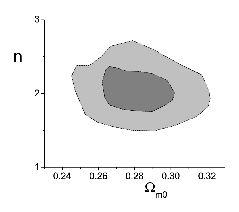
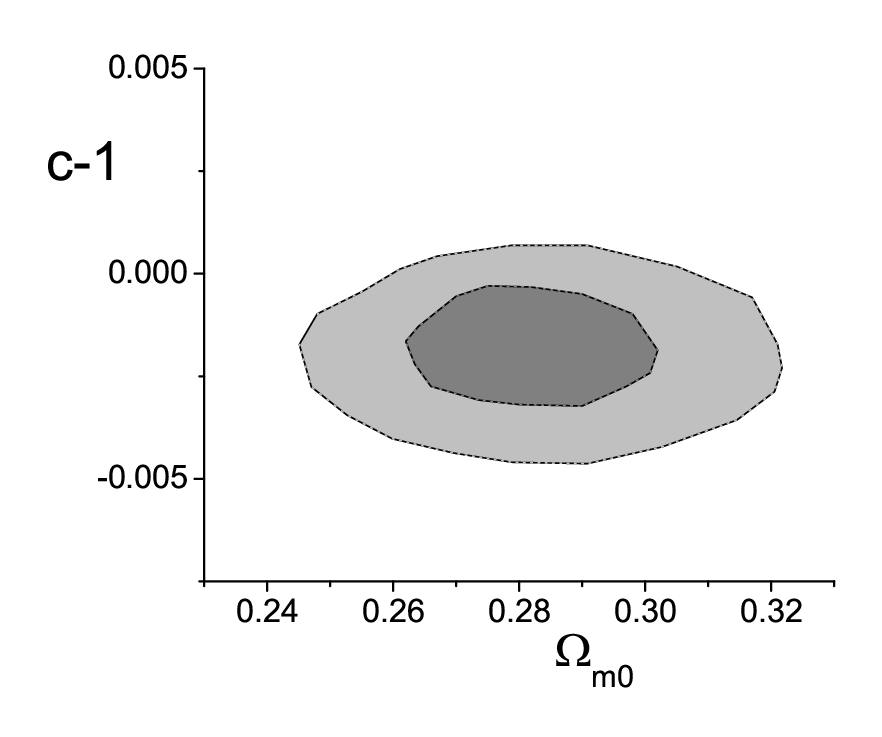
In Fig. 2 we provide the contour plots for the parameters and in terms of the current value of the matter density parameter , for the scenario of modified cosmology through non-extensive thermodynamics with varying exponent, using SNIa and data. As we can see the agreement with the data is very good, and the matter energy density coincides with that of Planck within 1 Ade:2015xua. For the new parameters of the scenario at hand we observe that they acquire values near their CDM ones, namely and (i.e. ). Nevertheless, is away from its CDM value at 1 confidence level, which shows that a slight deviation might be favored, however CDM paradigm is included within 2. Additionally, we mention that if we restrict our fittings to the case of , then we acquire at 1 , however with a large . Finally, we would like to mention that the incorporation of Cosmic Microwave Background (CMB) data, although necessary, requires a highly non-trivial treatment of the form, which in the model at hand in general cannot be obtained analytically. Such a detailed elaboration lies beyond the scope of the present analysis.
III.2 Early-time universe
In this subsection we study the modified Friedmann equation from non-extensive thermodynamics with varying exponent, namely Eq. (23), at early times, namely we desire to examine the inflationary realization. In this regime we may use the approximation , i.e. . Thus, in the case Eq. (23) becomes
| (41) |
while in the case and , we find
| (42) |
Hence, neglecting the matter sector, Eqs. (41),(42) give rise to inflationary de Sitter solutions. In particular, for we obtain
| (43) |
while for and we find
| (44) |
As we see, the scenario at hand accept inflationary de Sitter solutions at early times. In particular, from (43),(44) we may define an effective cosmological constant, namely
| (45) |
for , and
| (46) |
for , . Hence, the interesting feature of these solutions is that the cosmological constant is effectively screened, and the effective cosmological constant that drives inflation includes additionally the information of the new terms of non-extensive thermodynamics. This feature can be a great advantage in providing a description of both inflation and late-time acceleration with the same parameter choices, since the above effective screening gives the necessary enhanced acceleration in inflation comparing to dark-energy epoch.
As an illustrative example we consider the case . Then, in the early universe relation (44) gives , while at late times relation (36) results to . Hence, knowing that in the late-time universe while in the early universe , we find that e.g. for and and with , both regimes can be obtained simultaneously.
IV gravity correspondence
In this section we investigate the correspondence of modified cosmology through non-extensive thermodynamics with othe classes of modified gravity, and in particular with gravity. As we showed in subsection II.1, starting from the first law of thermodynamics and using the standard Bekenstein-Hawking entropy, one can result to the standard Friedmann equations. On the other hand, the use of non-extensive Tsallis entropy leads to modified Friedmann equations. Hence, the question is whether there is a correspondence of these modified Friedmann equations with the modified Friedmann equations arising from modified gravity theories such as gravity.
The action of gravity, alongside the matter sector, reads as
| (47) |
where is a function of the scalar curvature and is the matter action. Extracting the field equations and applying them in FRW geometry we obtain the corresponding Friedmann equations, namely Nojiri:2006gh
| (48) | ||||
| (49) |
Now, combining the general equations (5), (6), and (8), we obtain
| (50) |
Thus, substituting from (IV) into (50) we acquire the entropy as
| (51) |
Using that and , the above entropy expression can be written as
| (52) |
Note that, as expected, in case of Einstein gravity , the above result reproduces the standard result for the entropy, namely
| (53) |
where the second equality arises using that and that .
We focus on the de Sitter universe, in which is a constant. In this case expression (IV) reduces to
| (54) |
Interestingly enough, this is the standard result for the entropy in gravity, obtained in Brevik:2004sd; Cognola:2005de using the classical Euclidean action or the Noether charge method Iyer:1994ys in the de Sitter space-time. Hence, recalling that in a de Sitter universe and that , we find that . Therefore, if we consider the model where is given by the power of , namely , we deduce that (54) gives
| (55) |
Thus, making the identification
| (56) |
then the non-extensive Tsallis entropy is reproduced, and we obtain a correspondence between gravity and cosmology from non-extensive thermodynamics. As expected, when gravity becomes general relativity, i.e. for , (56) gives and standard thermodynamics with standard Friedmann equations are reproduced. Lastly, we mention here that the above simple correspondence has been shown in the case of a de Sitter universe. For more complicated geometries the correspondence is lost and modified cosmology from non-extensive thermodynamics does not have an equivalent gravity description, and hence it corresponds to a novel modification.
V Conclusions
In this work we investigated a modified cosmological scenario that arises from the application of non-extensive thermodynamics with varying exponent in a cosmological framework. In particular, it is known that one can apply the first law of thermodynamics in the universe apparent horizon and obtain the Friedmann equations. Nevertheless, in non-additive systems such as gravitational ones, the usual Bekenstein-Hawking entropy should be replaced by the generalized, non-extensive Tsallis entropy. Doing so we obtained modified Friedmann equations, which contain new terms quantified by the non-extensive exponent . Finally, following quantum considerations, we allowed to have a dependence on the scale, with the value 1 corresponding to standard thermodynamics and standard CDM cosmology.
Concerning the universe evolution at late times, the new terms that appear due to the non-extensive varying exponent constitute an effective dark energy sector. As we showed, the universe exhibits the usual thermal history, with the successive sequence of matter and dark-energy epochs, and with the transition to acceleration happening around in agreement with the observed behavior. Concerning the effective dark-energy equation-of-state parameter, we saw that it acquires values close to at present, while in the past it may lie either in the quintessence or in the phantom regime. The interesting feature is that the above behaviors can be obtained even if the explicit cosmological constant is set to zero, namely they arise purely from the extra terms in the Friedmann equations.
Confronting the model with SNIa and observational data, we provided the corresponding contour plots, and we showed that the agreement is very good. For the new parameters of the scenario at hand we saw that although there is a tendency for a slight deviation from the CDM values, CDM paradigm is included within 2.
In the early-time universe we saw that the scenario at hand can lead to inflationary de Sitter solutions, which are driven by an effective cosmological constant that includes additionally the information of the new terms of non-extensive thermodynamics. This feature can provide a description of both inflation and late-time acceleration with the same parameter choices, since the above effective screening gives the necessary enhanced acceleration in inflation comparing to dark-energy epoch. This is an advantage comparing to other models of the literature, which in general cannot describe inflation and late-time acceleration simultaneously since they cannot provide a natural change of the involved parameter scales.
Finally, we investigated the correspondence of the scenario at hand with modifications of gravity such as the gravity. As we showed, in the case of a de Sitter universe there is a correspondence between cosmology from non-extensive thermodynamics and power-law gravity, where the non-extensive exponent is related to the exponent. However, for more complicated geometries the correspondence is lost and the scenario at hand does not have an equivalent gravity description, forming a novel modification.
In summary, modified cosmology through non-extensive thermodynamics with varying exponent is very efficient in describing the universe evolution, from inflation to late-time acceleration. It would be interesting to perform further investigations on the scenario, such as a joint observational analysis using data from Type Ia Supernovae (SNIa), Baryon Acoustic Oscillations (BAO), Cosmic Microwave Background (CMB), and Hubble parameter observations, or a detailed phase-space analysis in order to extract the global features of the scenario. These necessary studies lie beyond the scope of this work and are left for future works.
Acknowledgements.
The authors would like to thank S. Pan and A. Mukherjee for useful comments. This article is based upon work from CANTATA COST (European Cooperation in Science and Technology) action CA15117, EU Framework Programme Horizon 2020. This work is also supported (in part) by MEXT KAKENHI Grant-in-Aid for Scientific Research on Innovative Areas gCosmic Accelerationh No. 15H05890 (S.N.) and the JSPS Grant-in-Aid for Scientific Research (C) No. 18K03615 (S.N.), and by MINECO (Spain), FIS2016-76363-P, and by project 2017 SGR247 (AGAUR, Catalonia) (S.D.O).References
- (1) P. J. E. Peebles and B. Ratra, Rev. Mod. Phys. 75, 559 (2003) [astro-ph/0207347].
- (2) Y. -F. Cai, E. N. Saridakis, M. R. Setare and J. -Q. Xia, Phys. Rept. 493, 1 (2010) [arXiv:0909.2776 [hep-th]].
- (3) N. Bartolo, E. Komatsu, S. Matarrese and A. Riotto, Phys. Rept. 402, 103 (2004) [astro-ph/0406398].
- (4) S. Nojiri and S. D. Odintsov, Phys. Rev. D 68, 123512 (2003) [hep-th/0307288].
- (5) S. Nojiri and S. D. Odintsov, eConf C 0602061, 06 (2006) [Int. J. Geom. Meth. Mod. Phys. 4, 115 (2007)] [hep-th/0601213].
- (6) S. Capozziello and M. De Laurentis, Phys. Rept. 509, 167 (2011) [arXiv:1108.6266 [gr-qc]].
- (7) Y. F. Cai, S. Capozziello, M. De Laurentis and E. N. Saridakis, Rept. Prog. Phys. 79, 106901 (2016) [arXiv:1511.07586 [gr-qc]].
- (8) S. Capozziello, Int. J. Mod. Phys. D 11, 483 (2002) [gr-qc/0201033].
- (9) S. Nojiri and S. D. Odintsov, Phys. Rev. D 74, 086005 (2006) [hep-th/0608008].
- (10) S. Nojiri and S. D. Odintsov, Phys. Rept. 505, 59 (2011) [arXiv:1011.0544 [gr-qc]].
- (11) S. Nojiri and S. D. Odintsov, Phys. Lett. B 631, 1 (2005) [hep-th/0508049].
- (12) P. D. Mannheim and D. Kazanas, Astrophys. J. 342, 635 (1989).
- (13) E. E. Flanagan, Phys. Rev. D 74, 023002 (2006) [astro-ph/0605504].
- (14) A. Nicolis, R. Rattazzi and E. Trincherini, Phys. Rev. D 79, 064036 (2009) [arXiv:0811.2197 [hep-th]].
- (15) C. Deffayet, G. Esposito-Farese and A. Vikman, Phys. Rev. D 79, 084003 (2009) [arXiv:0901.1314 [hep-th]].
- (16) G. Leon and E. N. Saridakis, JCAP 1303, 025 (2013) [arXiv:1211.3088 [astro-ph.CO]].
- (17) G. R. Bengochea and R. Ferraro, Phys. Rev. D 79, 124019 (2009) [arXiv:0812.1205 [astro-ph]].
- (18) S. H. Chen, J. B. Dent, S. Dutta and E. N. Saridakis, Phys. Rev. D 83, 023508 (2011) [arXiv:1008.1250 [astro-ph.CO]].
- (19) G. Kofinas and E. N. Saridakis, Phys. Rev. D 90, 084044 (2014) [arXiv:1404.2249 [gr-qc]].
- (20) G. Kofinas and E. N. Saridakis, Phys. Rev. D 90, 084045 (2014) [arXiv:1408.0107 [gr-qc]].
- (21) T. Jacobson, Phys. Rev. Lett. 75, 1260 (1995) [gr-qc/9504004].
- (22) T. Padmanabhan, Phys. Rept. 406, 49 (2005) [gr-qc/0311036].
- (23) T. Padmanabhan, Rept. Prog. Phys. 73, 046901 (2010) [arXiv:0911.5004 [gr-qc]].
- (24) R. G. Cai and S. P. Kim, JHEP 0502, 050 (2005) [arXiv:hep-th/0501055].
- (25) M. Akbar and R. G. Cai, Phys. Rev. D 75, 084003 (2007) [hep-th/0609128].
- (26) R. G. Cai and L. M. Cao, Phys. Rev. D 75, 064008 (2007) [gr-qc/0611071].
- (27) A. Paranjape, S. Sarkar and T. Padmanabhan, Phys. Rev. D 74, 104015 (2006) [hep-th/0607240].
- (28) A. Sheykhi, B. Wang and R. G. Cai, Nucl. Phys. B 779, 1 (2007) [arXiv:hep-th/0701198].
- (29) M. Akbar and R. G. Cai, Phys. Lett. B 635, 7 (2006) [hep-th/0602156].
- (30) M. Jamil, E. N. Saridakis and M. R. Setare, Phys. Rev. D 81, 023007 (2010) [arXiv:0910.0822 [hep-th]].
- (31) R. G. Cai and N. Ohta, Phys. Rev. D 81, 084061 (2010) [arXiv:0910.2307 [hep-th]].
- (32) M. Wang, J. Jing, C. Ding and S. Chen, Phys. Rev. D 81, 083006 (2010) [arXiv:0912.4832 [gr-qc]].
- (33) M. Jamil, E. N. Saridakis and M. R. Setare, JCAP 1011, 032 (2010) [arXiv:1003.0876 [hep-th]].
- (34) Y. Gim, W. Kim and S. H. Yi, JHEP 1407, 002 (2014) [arXiv:1403.4704 [hep-th]].
- (35) Z. Y. Fan and H. Lu, Phys. Rev. D 91, no. 6, 064009 (2015) [arXiv:1501.00006 [hep-th]].
- (36) C. Tsallis and L. J. L. Cirto, Eur. Phys. J. C 73, 2487 (2013) [arXiv:1202.2154 [cond-mat.stat-mech]].
- (37) N. Komatsu and S. Kimura, Phys. Rev. D 88, 083534 (2013) [arXiv:1307.5949 [astro-ph.CO]].
- (38) E. M. Barboza, Jr., R. d. C. Nunes, E. M. C. Abreu and J. Ananias Neto, Physica A 436, 301 (2015) [arXiv:1403.5706 [gr-qc]].
- (39) A. Lymperis and E. N. Saridakis, Eur. Phys. J. C 78, no. 12, 993 (2018) [arXiv:1806.04614 [gr-qc]].
- (40) E. N. Saridakis, K. Bamba, R. Myrzakulov and F. K. Anagnostopoulos, JCAP 1812, no. 12, 012 (2018) [arXiv:1806.01301 [gr-qc]].
- (41) A. Sheykhi, Phys. Lett. B 785, 118 (2018) [arXiv:1806.03996 [gr-qc]].
- (42) M. Artymowski and J. Mielczarek, arXiv:1806.03924 [gr-qc].
- (43) E. M. C. Abreu, J. A. Neto, A. C. R. Mendes and A. Bonilla, EPL 121, no. 4, 45002 (2018) [arXiv:1711.06513 [gr-qc]].
- (44) A. Jawad and A. Iqbal, doi:10.1142/S021988781850130X
- (45) M. Abdollahi Zadeh, A. Sheykhi and H. Moradpour, arXiv:1810.12104 [physics.gen-ph].
- (46) W. J. C. da Silva and R. Silva, arXiv:1810.03759 [astro-ph.CO].
- (47) C. Tsallis, J. Statist. Phys. 52 (1988) 479.
- (48) M. L. Lyra and C. Tsallis, Phys. Rev. Lett. 80, 53 (1998).
- (49) G. Wilk and Z. Wlodarczyk, Phys. Rev. Lett. 84, 2770 (2000) [hep-ph/9908459].
- (50) R. G. Cai, L. M. Cao and Y. P. Hu, Class. Quant. Grav. 26, 155018 (2009) [arXiv:0809.1554 [hep-th]].
- (51) D. Bak and S. J. Rey, Class. Quant. Grav. 17, L83 (2000) [hep-th/9902173].
- (52) S. A. Hayward, Class. Quant. Grav. 15, 3147 (1998) [gr-qc/9710089].
- (53) S. A. Hayward, S. Mukohyama and M. C. Ashworth, Phys. Lett. A 256, 347 (1999) [gr-qc/9810006].
- (54) M. Li, Phys. Lett. B 603, 1 (2004) [hep-th/0403127].
- (55) W. Fischler and L. Susskind, hep-th/9806039.
- (56) S. Nojiri and S. D. Odintsov, Gen. Rel. Grav. 38 (2006) 1285 [hep-th/0506212].
- (57) P. A. R. Ade et al. [Planck Collaboration], Astron. Astrophys. 594, A13 (2016) [arXiv:1502.01589 [astro-ph.CO]].
- (58) D. Foreman-Mackey, D. W. Hogg, D. Lang and J. Goodman, Publ. Astron. Soc. Pac. 125, 306 (2013) [arXiv:1202.3665 [astro-ph.IM]].
- (59) D. M. Scolnic et al., Astrophys. J. 859, no. 2, 101 (2018) [arXiv:1710.00845 [astro-ph.CO]].
- (60) H. Yu, B. Ratra and F. Y. Wang, Astrophys. J. 856, no. 1, 3 (2018) [arXiv:1711.03437 [astro-ph.CO]].
- (61) R. C. Nunes, S. Pan and E. N. Saridakis, JCAP 1608, no. 08, 011 (2016) [arXiv:1606.04359 [gr-qc]].
- (62) R. C. Nunes, S. Pan, E. N. Saridakis and E. M. C. Abreu, JCAP 1701, no. 01, 005 (2017) [arXiv:1610.07518 [astro-ph.CO]].
- (63) F. K. Anagnostopoulos and S. Basilakos, Phys. Rev. D 97, no. 6, 063503 (2018) [arXiv:1709.02356 [astro-ph.CO]].
- (64) S. Basilakos, S. Nesseris, F. K. Anagnostopoulos and E. N. Saridakis, JCAP 1808, no. 08, 008 (2018) [arXiv:1803.09278 [astro-ph.CO]].
- (65) I. H. Brevik, S. Nojiri, S. D. Odintsov and L. Vanzo, Phys. Rev. D 70 (2004) 043520 [hep-th/0401073].
- (66) G. Cognola, E. Elizalde, S. Nojiri, S. D. Odintsov and S. Zerbini, JCAP 0502 (2005) 010 [hep-th/0501096].
- (67) V. Iyer and R. M. Wald, Phys. Rev. D 50 (1994) 846 [gr-qc/9403028].