Label Embedded Dictionary Learning for Image ClassificationJournal: Neurocomputing

SRC was proposed by Wright et al. 2009. Assume that we have $C$ classes of training samples, denoted by ${{\mathbf{X}}_{c}},c=1,2,\cdots,C$, where ${{\mathbf{X}}_{c}}$ is the training sample matrix of class $c$. Each column of the matrix ${{\mathbf{X}}_{c}}$ is a training sample feature from the $c_{th}$ class. The whole training sample matrix can be denoted as $\mathbf{X}=\left[{{\mathbf{X}}_{1}},{{\mathbf{X}}_{2}},\cdots{{\mathbf{X}}_{C}}\right]\in{{\mathbb{R}}^{D\times N}}$, where $D$ represents the dimensions of the sample features and $N$ is the number of training samples. Supposing that $\mathbf{y}\in{{\mathbb{R}}^{D\times 1}}$ is a testing sample vector, the sparse representation algorithm aims to solve the following objective function:

where, $\alpha$ is the regularization parameter to control the tradeoff between fitting goodness and sparseness. The sparse representation based classification is to find the minimum value of the residual error for each class.

where $id\left(\bf{y}\right)$ represents the predictive label of $\bf{y}$, ${{{\bf{\hat{s}}}}_{c}}$ is the sparse code of $c_{th}$ class. The procedure of SRC is shown in Algorithm 1. Obviously, the residual $e_{c}$ is associated with only a few images in class $c$.

Jiang et al. 2013 proposed LC-KSVD to encourage the similarity among representations of samples belonging to the same class in D-KSVD. The authors proposed to combine the discriminative sparse codes error with the reconstruction error and the classification error to form a unified objective function, which gave discriminative sparse codes matrix ${\bf{Q}}=\left[{{{\bf{q}}_{1}},{{\bf{q}}_{2}},\cdots,{{\bf{q}}_{N}}}\right]\in{{\mathbb{R}}^{K\times N}}$, label matrix ${\bf{H}}=\left[{{{\bf{h}}_{1}},{{\bf{h}}_{2}},\cdots,{{\bf{h}}_{N}}}\right]\in{{\mathbb{R}}^{C\times N}}$ and training sample matrix ${\bf{X}}$. The objective function is defined as follows:

where $T$ is the sparsity constraint factor, making sure that ${{{\bf{s}}_{i}}}$ has no more than $T$ nonzero entries. The dictionary ${\bf{B}}=\left[{{{\bf{b}}_{1}},{{\bf{b}}_{2}},\cdots,{{\bf{b}}_{K}}}\right]\in{{\mathbb{R}}^{D\times K}}$, where $K>D$ is the number of atoms in the dictionary, and ${\bf{S}}=\left[{{{\bf{s}}_{1}},{{\bf{s}}_{2}},\cdots,{{\bf{s}}_{N}}}\right]\in{{\mathbb{R}}^{K\times D}}$ is the sparse codes of training sample matrix ${\bf{X}}$. ${\bf{W}}=\left[{{{\bf{w}}_{1}},{{\bf{w}}_{2}},\cdots,{{\bf{w}}_{K}}}\right]\\ \in{{\mathbb{R}}^{C\times K}}$ is a classifier learned from the given label matrix ${\bf{H}}$. We hope the ${\bf{W}}$ can return the most probable class this sample belongs to. ${\bf{A}}=\left[{{{\bf{a}}_{1}},{{\bf{a}}_{2}},\cdots,{{\bf{a}}_{K}}}\right]\in{{\mathbb{R}}^{K\times K}}$ is a linear transformation relys on ${\bf{Q}}$. $\lambda$ and $\omega$ are the regularization parameters balancing the discriminative sparse codes error and the classification contribution to the overall objective, respectively. The algorithm is shown in Algorithm 2. Here, we denote $m\left({m=0,1,2,\cdots}\right)$ as the iteration number and ${\left(\bullet\right)_{m}}$ means the value of matrix $\left(\bullet\right)$ after ${m_{th}}$ iteration.

While the LC-KSVD algorithm exploits the $\ell_{0}$-norm regularization term to control the sparseness, it is difficult to find the optimal sparse solution to a general image recognition. The reason is that LC-KSVD use OMP method to optimise the objective function which usually obtain the suboptimal sparse solution unless finding the perfect initialized values.

Motivated by that the optimal sparse solution can not be found easily with $\ell_{0}$-norm regularization term, we propose a novel dictionary learning method named label embedded dictionary learning (LEDL) for image classification. This method introduces the $\ell_{1}$-norm regularization term to replace the $\ell_{0}$-norm regularization of LC-KSVD. Thus, we can freely select the basis vectors for linear fitting to get optimal sparse solution. The objection function is as follows:

where, ${\left(\bullet\right)_{\bullet k}}$ denotes the $k_{th}$ column vector of matrix $\left(\bullet\right)$. The $\ell_{1}$-norm regularization term is utilized to enforce sparsity and $\varepsilon$ is the regularization parameter which has the same function as $\alpha$ in Equation (1).

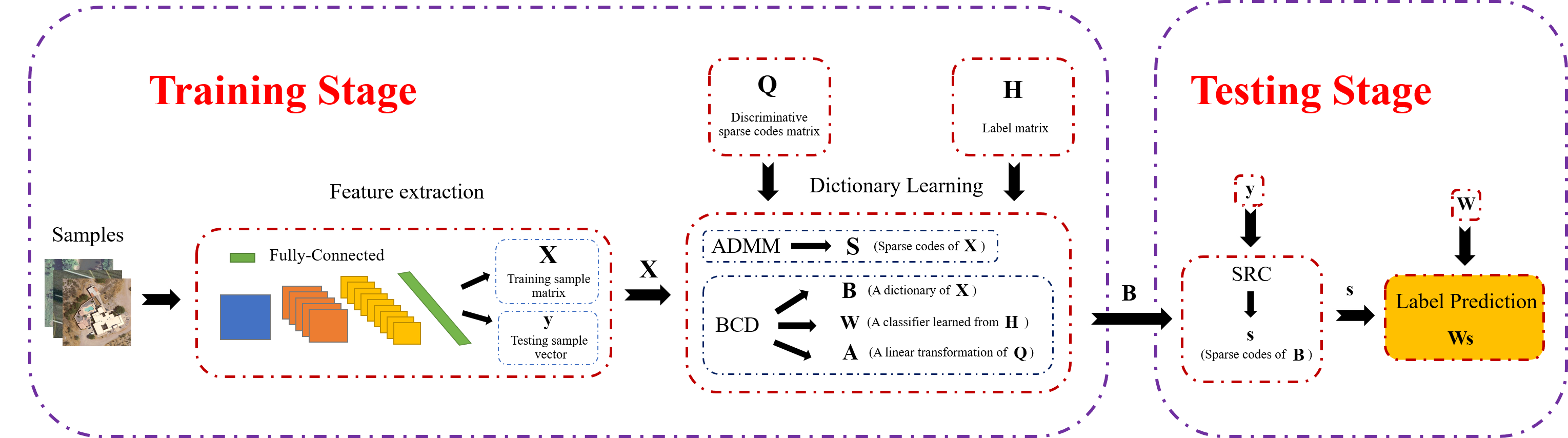
Consider the optimization problem (4) is not jointly convex in both ${\bf{S}}$, ${\bf{B}}$, ${\bf{W}}$ and ${\bf{A}}$, it is separately convex in either ${\bf{S}}$ (with ${\bf{B}}$, ${\bf{W}}$, ${\bf{A}}$ fixed), ${\bf{B}}$ (with ${\bf{S}}$, ${\bf{W}}$, ${\bf{A}}$ fixed), ${\bf{W}}$ (with ${\bf{S}}$, ${\bf{B}}$, ${\bf{A}}$ fixed) or ${\bf{A}}$ (with ${\bf{S}}$, ${\bf{B}}$, ${\bf{W}}$ fixed). To this end, the optimization problem can be recognised as four optimization subproblems which are finding sparse codes ($\bf{S}$) and learning bases ($\bf{B}$, $\bf{W}$, $\bf{A}$), respectively. Here, we employ the alternating direction method of multipliers (ADMM) Boyd et al. 2011 framework to solve the first subproblem and the blockwise coordinate descent (BCD) Liu et al. 2014b algorithm for the rest subproblem. The complete process of LEDL is shown in Figure 2.

For all the datasets, in order to eliminate the randomness, we carry out every experiment 8 times and the mean of the classification rates is reported. And we randomly select 5 samples per class for training in all the experiments. For Extended YaleB dataset and CMU PIE dataset, each image is cropped to $32\times 32$, pulled into column vector, and $\ell_{2}$ normalized to form the raw $\ell_{2}$ normalized features. For UC Merced Land Use dataset, AID dataset, we use resnet model He et al. 2016 to extract the features. Specifically, the layer $pool5$ is utilized to extract 2048-dimensional vectors for them. For Caltech101 dataset, we use the layer $pool5$ of resnet model and spatial pyramid matching (SPM) with two layers (the second layer include five part, such as left upper, right upper, left lower, right lower, center) to extract 12288-dimensional vectors. And finally, each of the images in USPS dataset is resized into $16\times 16$ vectors.

For convenience, the dictionary size ($K$) is fixed to the twice the number of training samples. In addition, we set $\rho=1$ and initial $\theta=0.5$, then decrease the $\theta$ in each iteration. Moreover, there are other three parameters ($\lambda$, $\omega$ and $\varepsilon$) need to be adjust to achieve the highst classification rates. The details are showed in the following subsections.

The Extended YaleB dataset contains $2{,}432$ face images from 38 individuals, each having 64 frontal images under varying illumination conditions. Figure 4 shows some images of the dataset.

In addition, we set $\lambda={2^{-3}}$, $\omega={2^{-11}}$, $\varepsilon={2^{-8}}$ in our experiment. The experimental results are summarized in Table (1). We can see that our proposed LEDL algorithm achieves superior performance to other classical classification methods by an improvement of at least $1.1$$\%$. Compared with $\ell_{0}$-norm sparsity constraint based dictionary learning algorithm LC-KSVD, our proposed $\ell_{1}$-norm sparsity constraint based dictionary learning algorithm LEDL algorithm exceeds it $7.8$$\%$. The reason of the high improvement between LC-KSVD and LEDL is that $\ell_{0}$-norm sparsity constraint leads to NP-hard problem which is not conductive to finding the optimal sparse solution for the dictionary. In order to further illustrate the performance of our method, we choose the first 20 classes samples as a subdataset and show the confusion matrices in Figure 5. As can be seen that, our method achieves higher classification rates in all the chosen $20$ classes than LC-KSVD. Especially in class1, class2, class3, class10, class16, LEDL can achieve at least $10.0$$\%$ performance gain than LC-KSVD.

The CMU PIE dataset consists of $41{,}368$ images of 68 individuals with 43 different illumination conditions. Each human is under 13 different poses and with 4 different expressions. In Figure 6, we list several samples from this dataset.

The comparasion results are showed in Table 1, we can see that our proposed LEDL algorithm outperforms over other well-known methods by an improvement of at least $0.5$$\%$. To be attention, LEDL is capable of exceeding LC-KSVD $10.6$$\%$ in this dataset. The optimal parameters are $\lambda={2^{-3}}$, $\omega={2^{-11}}$, $\varepsilon={2^{-8}}$.

The UC Merced Land Use dataset is widely used for aerial image classification. It consists of totally $2{,}100$ land-use images of $21$ classes. Some samples are showed in Figure 7.

In Table 1, we can see that our proposed LEDL algorithm is only similar with CRC and still outperforms the other methods. Compared with LC-KSVD, LEDL achieves the higher accuracy by an improvement of $1.3$$\%$. Here, we set $\lambda={2^{0}}$, $\omega={2^{-9}}$, $\varepsilon={2^{-6}}$ to get the optimal result. The confusion matrices of the UC Merced Land Use dataset for all classes are shown in Figure 8. We can see that, in all classes except the tennis, LEDL almost achieve better results compared with LC-KSVD. In several classes such as building, freeway, river, and sparse, our method achieves superior performance to LC-KSVD by an improvement of at least $0.5$$\%$.

The AID dataset is a new large-scale aerial image dataset which can be downloaded from Google Earth imagery. It contains $10{,}000$ images from 30 aerial scene types. In Figure 9, we show several images of this dataset.

Table 1 illustrates the effectiveness of LEDL for classifying images. We adjust $\lambda={2^{-6}}$, $\omega={2^{-14}}$, $\varepsilon={2^{-12}}$ to achieve the highest accuracy by an improvement of at least $0.3$$\%$ in the five algorithms. While compared with LC-KSVD, LEDL achieves an improvement of $2.7$$\%$.

The caltech101 dataset includes $9{,}144$ images of $102$ classes in total, which are consisted of cars, faces, flowers and so on. Each category have about 40 to 800 images and most of them have about 50 images. In figure 10, we show several images of this dataset.

As can be seen in Table 1, our proposed LEDL algorithm outperforms all the competing approaches by setting $\lambda={2^{-4}}$, $\omega={2^{-13}}$, $\varepsilon={2^{-14}}$ and achieves improvements of $1.8$$\%$ and $0.7$$\%$ over LC-KSVD and other methods, respectively. Here, we also choose the first 20 classes to build the confusion matrices. They are shown in Figure 11.

The USPS dataset contains $9{,}298$ handwritten digit images from 0 to 9 which come from the U.S. Postal System. We list several samples from this dataset in Figure 12.

Table 1 shows the comparasion results of five algorithms and it is easy to find out that our proposed LEDL algorithm outperforms over other well-known methods by an improvement of at least $2.3$$\%$. And our proposed method achieves an improvement of $10.0$$\%$ over LC-KSVD method. The optimal parameters are $\lambda={2^{-4}}$, $\omega={2^{-8}}$, $\varepsilon={2^{-5}}$.

From the experimental results on six datasets, we can obtain the following conclusions.

(1) All the above experimental results illustrate that, our proposed LEDL algorithm is an effective and general classifier which can achieve superior performacne to state-of-the-art methods on various datasets, especially on Extended YaleB dataset, CMU PIE dataset and USPS dataset.

(2) Our proposed LEDL method introduces the $\ell_{1}$-norm regularization term to replace the $\ell_{0}$-norm regularization of LC-KSVD. However, compared with LC-KSVD algorithm, LEDL method is always better than it on the six datasets. Moreover, on the two face datasets and USPS dataset, our method can exceed LC-KSVD nearly $10.0$$\%$.

(3) Confusion matrices of LEDL and LC-KSVD on three datasets are shown in Figure 5 8 and 11. They clearly illustrate the superiority of our method. Specificially, for Extended YaleB dataset, our method achieve outstanding performance in five classes (class1, class2, class3, class10, class16). For UC Merced dataset, LEDL almost achieve better classification rates than LC-KSVD in all classes except the tennis class. For Caltech101 dataset, our proposed LEDL method perform much better than LC-KSVD method in some classes such as beaver, binocular, brontosaurus, cannon and ceiling fan.

References

- Aharon et al. (2006) Aharon, M., Elad, M., Bruckstein, A., et al., 2006. K-svd: An algorithm for designing overcomplete dictionaries for sparse representation. IEEE Transactions on signal processing 54 (11), 4311–4322.
- Boyd et al. (2011) Boyd, S., Parikh, N., Chu, E., Peleato, B., Eckstein, J., 2011. Distributed optimization and statistical learning via the alternating direction method of multipliers. Foundations and Trends® in Machine learning 3 (1), 1–122.
- Chan et al. (2015) Chan, T.-H., Jia, K., Gao, S., Lu, J., Zeng, Z., Ma, Y., 2015. Pcanet: A simple deep learning baseline for image classification? IEEE Transactions on image processing 24 (12), 5017–5032.
- Chang et al. (2016) Chang, H., Yang, M., Yang, J., 2016. Learning a structure adaptive dictionary for sparse representation based classification. Neurocomputing 190 (19), 124–131.
- Chang et al. (2000) Chang, S. G., Yu, B., Vetterli, M., 2000. Adaptive wavelet thresholding for image denoising and compression. IEEE Transactions on image processing 9 (9), 1532–1546.
- Fei-Fei et al. (2007) Fei-Fei, L., Fergus, R., Perona, P., 2007. Learning generative visual models from few training examples: An incremental bayesian approach tested on 101 object categories. Computer vision and Image understanding 106 (1), 59–70.
- Gao et al. (2018) Gao, D., Hu, Z., Ye, R., 2018. Self-dictionary regression for hyperspectral image super-resolution. Remote Sensing 10 (10), 1574–1596.
- Georghiades et al. (2001) Georghiades, A. S., Belhumeur, P. N., Kriegman, D. J., 2001. From few to many: Illumination cone models for face recognition under variable lighting and pose. IEEE Transactions on pattern analysis and machine intelligence 23 (6), 643–660.
- Hao et al. (2017) Hao, S., Wang, W., Yan, Y., Bruzzone, L., 2017. Class-wise dictionary learning for hyperspectral image classification. Neurocomputing 220 (12), 121–129.
- He et al. (2016) He, K., Zhang, X., Ren, S., Sun, J., 2016. Deep residual learning for image recognition. In: Computer Vision and Pattern Recognition (CVPR), 2016 IEEE conference on. IEEE, pp. 770–778.
- Hull (1994) Hull, J. J., 1994. A database for handwritten text recognition research. IEEE Transactions on pattern analysis and machine intelligence 16 (5), 550–554.
- Ji et al. (2014) Ji, R., Gao, Y., Hong, R., Liu, Q., Tao, D., Li, X., 2014. Spectral-spatial constraint hyperspectral image classification. IEEE Transactions on geoscience and remote sensing 52 (3), 1811–1824.
- Jiang et al. (2013) Jiang, Z., Lin, Z., Davis, L. S., 2013. Label consistent k-svd: Learning a discriminative dictionary for recognition. IEEE Transactions on pattern analysis and machine intelligence 35 (11), 2651–2664.
- Li et al. (2018) Li, H., He, X., Tao, D., Tang, Y., Wang, R., 2018. Joint medical image fusion, denoising and enhancement via discriminative low-rank sparse dictionaries learning. Pattern Recognition 79, 130–146.
- Li et al. (2012) Li, S., Fang, L., Yin, H., 2012. An efficient dictionary learning algorithm and its application to 3-d medical image denoising. IEEE Transactions on biomedical engineering 59 (2), 417–427.
- Liu et al. (2017) Liu, B.-D., Gui, L., Wang, Y., Wang, Y.-X., Shen, B., Li, X., Wang, Y.-J., 2017. Class specific centralized dictionary learning for face recognition. Multimedia Tools and Applications 76 (3), 4159–4177.
- Liu et al. (2016) Liu, B.-D., Shen, B., Gui, L., Wang, Y.-X., Li, X., Yan, F., Wang, Y.-J., 2016. Face recognition using class specific dictionary learning for sparse representation and collaborative representation. Neurocomputing 204 (5), 198–210.
- Liu et al. (2014a) Liu, B.-D., Shen, B., Wang, Y.-X., 2014a. Class specific dictionary learning for face recognition. In: Security, Pattern Analysis, and Cybernetics (SPAC), 2014 IEEE International conference on. IEEE, pp. 229–234.
- Liu et al. (2014b) Liu, B.-D., Wang, Y.-X., Shen, B., Zhang, Y.-J., Wang, Y.-J., 2014b. Blockwise coordinate descent schemes for sparse representation. In: Acoustics, Speech and Signal Processing (ICASSP), 2014 IEEE International conference on. IEEE, pp. 5267–5271.
- Mallat and Zhang (1993) Mallat, S. G., Zhang, Z., 1993. Matching pursuit with time-frequency dictionaries. IEEE Transactions on signal processing 41 (12), 3397–3415.
- Nakazawa and Kulkarni (2018) Nakazawa, T., Kulkarni, D. V., 2018. Wafer map defect pattern classification and image retrieval using convolutional neural network. IEEE Transactions on semiconductor manufacturing 31 (2), 309–314.
- Natarajan (1995) Natarajan, B. K., 1995. Sparse approximate solutions to linear systems. SIAM journal on computing 24 (2), 227–234.
- Olshausen and Field (1996) Olshausen, B. A., Field, D. J., 1996. Emergence of simple-cell receptive field properties by learning a sparse code for natural images. Nature 381 (6583), 607–609.
- Olshausen and Field (1997) Olshausen, B. A., Field, D. J., 1997. Sparse coding with an overcomplete basis set: a strategy employed by v1? Vision Research 37 (23), 3311–3325.
- Shi et al. (2018) Shi, H., Zhang, Y., Zhang, Z., Ma, N., Zhao, X., Gao, Y., Sun, J., 2018. Hypergraph-induced convolutional networks for visual classification. IEEE Transactions on neural networks and learning systems.
- Sim et al. (2002) Sim, T., Baker, S., Bsat, M., 2002. The cmu pose, illumination, and expression (pie) database. In: Automatic Face and Gesture Recognition (FG), 2002 IEEE International conference on. IEEE, pp. 53–58.
- Song et al. (2018) Song, Y., Liu, Y., Gao, Q., Gao, X., Nie, F., Cui, R., 2018. Euler label consistent k-svd for image classification and action recognition. Neurocomputing 310 (8), 277–286.
- Tropp and Gilbert (2007) Tropp, J. A., Gilbert, A. C., 2007. Signal recovery from random measurements via orthogonal matching pursuit. IEEE Transactions on information theory 53 (12), 4655–4666.
- Wang et al. (2012a) Wang, H., Yuan, C., Hu, W., Sun, C., 2012a. Supervised class-specific dictionary learning for sparse modeling in action recognition. Pattern Recognition 45 (11), 3902–3911.
- Wang et al. (2018) Wang, N., Zhao, X., Jiang, Y., Gao, Y., BNRist, K., 2018. Iterative metric learning for imbalance data classification. In: International Joint Conference on Artificial Intelligence (IJCAI), 2018 Morgan Kaufmann conference on. Morgan Kaufmann, pp. 2805–2811.
- Wang et al. (2012b) Wang, S., Zhang, L., Liang, Y., Pan, Q., 2012b. Semi-coupled dictionary learning with applications to image super-resolution and photo-sketch synthesis. In: Computer Vision and Pattern Recognition (CVPR), 2012 IEEE conference on. IEEE, pp. 2216–2223.
- Wright et al. (2009) Wright, J., Yang, A. Y., Ganesh, A., Sastry, S. S., Ma, Y., 2009. Robust face recognition via sparse representation. IEEE Transactions on pattern analysis and machine intelligence 31 (2), 210–227.
- Xia et al. (2017) Xia, G.-S., Hu, J., Hu, F., Shi, B., Bai, X., Zhong, Y., Zhang, L., Lu, X., 2017. Aid: A benchmark data set for performance evaluation of aerial scene classification. IEEE Transactions on geoscience and remote sensing 55 (7), 3965–3981.
- Xu et al. (2019) Xu, J., An, W., Zhang, L., Zhang, D., 2019. Sparse, collaborative, or nonnegative representation: Which helps pattern classification? Pattern Recognition 88, 679–688.
- Yang et al. (2010) Yang, J., Wright, J., Huang, T. S., Ma, Y., 2010. Image super-resolution via sparse representation. IEEE Transactions on image processing 19 (11), 2861–2873.
- Yang et al. (2009) Yang, J., Yu, K., Gong, Y., Huang, T., 2009. Linear spatial pyramid matching using sparse coding for image classification. In: Computer Vision and Pattern Recognition (CVPR), 2009 IEEE conference on. IEEE, pp. 1794–1801.
- Yang et al. (2017) Yang, M., Chang, H., Luo, W., 2017. Discriminative analysis-synthesis dictionary learning for image classification. Neurocomputing 219 (5), 404–411.
- Yang et al. (2014) Yang, M., Zhang, L., Feng, X., Zhang, D., 2014. Sparse representation based fisher discrimination dictionary learning for image classification. International Journal of Computer Vision 109 (3), 209–232.
- Yang and Newsam (2010) Yang, Y., Newsam, S., 2010. Bag-of-visual-words and spatial extensions for land-use classification. In: Advances in Geographic Information Systems (GIS), 2010 ACM International conference on. ACM, pp. 270–279.
- Yu et al. (2012a) Yu, J., Feng, L., Seah, H. S., Li, C., Lin, Z., 2012a. Image classification by multimodal subspace learning. Pattern Recognition Letters 33 (9), 1196–1204.
- Yu et al. (2014) Yu, J., Rui, Y., Tang, Y. Y., Tao, D., 2014. High-order distance-based multiview stochastic learning in image classification. IEEE Transactions on cybernetics 44 (12), 2431–2442.
- Yu et al. (2013) Yu, J., Tao, D., Rui, Y., Cheng, J., 2013. Pairwise constraints based multiview features fusion for scene classification. Pattern Recognition 46 (2), 483–496.
- Yu et al. (2012b) Yu, J., Tao, D., Wang, M., 2012b. Adaptive hypergraph learning and its application in image classification. IEEE Transactions on image processing 21 (7), 3262–3272.
- Yuan et al. (2016) Yuan, L., Liu, W., Li, Y., 2016. Non-negative dictionary based sparse representation classification for ear recognition with occlusion. Neurocomputing 171 (1), 540–550.
- Zhang et al. (2011) Zhang, L., Yang, M., Feng, X., 2011. Sparse representation or collaborative representation: Which helps face recognition? In: Computer Vision (ICCV), 2011 IEEE International conference on. IEEE, pp. 471–478.
- Zhang and Li (2010) Zhang, Q., Li, B., 2010. Discriminative k-svd for dictionary learning in face recognition. In: Computer Vision and Pattern Recognition (CVPR), 2010 IEEE conference on. IEEE, pp. 2691–2698.