跳到论文正文
W Papers独立论文阅读器 arXiv:1903.02833 论文正文 计算阅读时间 · 0%
引用这篇论文根据当前论文元数据生成,正式投稿前建议核对。


License: arXiv.org perpetual non-exclusive license
arXiv:1903.02833v3 [q-fin.MF] 30 Oct 2020

Asymptotics for volatility derivatives in multi-factor rough volatility modelsThanks: The authors are grateful to Antoine Jacquier, Mikko Pakkanen and Ryan McCrickerd for stimulating discussions. AM and HS thank the EPSRC CDT in Financial Computing and Analytics for financial support

Chloe Lacombe Address: Department of Mathematics, Imperial College London Email address: chloe.lacombe14@imperial.ac.uk , Aitor Muguruza Address: Department of Mathematics, Imperial College London and Synergis Email address: aitor.muguruza-gonzalez15@imperial.ac.uk and Henry Stone Address: Department of Mathematics, Imperial College London Email address: henry.stone15@imperial.ac.uk
Date: August 11, 2026
Abstract.

We study the small-time implied volatility smile for Realised Variance options, and investigate the effect of correlation in multi-factor models on the linearity of the smile. We also develop an approximation scheme for the Realised Variance density, allowing fast and accurate pricing of Volatility Swaps. Additionally, we establish small-noise asymptotic behaviour of a general class of VIX options in the large strike regime.

Key words and phrases: 
Rough volatility, VIX, large deviations, realised variance, small-time asymptotics, Gaussian measure, reproducing kernel Hilbert space.
2010 Mathematics Subject Classification
Primary 60F10, 60G22; Secondary 91G20, 60G15, 91G60

1. Introduction

Following the works by Alòs, León and Vives [ALV07], Gatheral, Jaisson, and Rosenbaum [GJR18] and Bayer, Friz and Gatheral [BFG16], rough volatility is becoming a new breed in financial modelling by generalising Bergomi’s ‘second generation’ stochastic volatility models to a non-Markovian setting. The most basic form of (lognormal) rough volatility model is the so-called rough Bergomi model introduced in [BFG16]. Gassiat [Gas18] recently proved that such a model (under certain correlation regimes) generates true martingales for the spot process. The lack of Markovianity imposes numerous fundamental theoretical questions and practical challenges in order to make rough volatility usable in an industrial environment. On the theoretical side, Jacquier, Pakkanen, and Stone [JPS18] prove a large deviations principle for a rescaled version of the log stock price process. In this same direction, Bayer, Friz, Gulisashvili, Horvath and Stemper [BFGHS17], Forde and Zhang [FZ17], Horvath, Jacquier and Lacombe [HJL18] and most recently Friz, Gassiat and Pigato [FGP18] (to name a few) prove large deviations principles for a wide range of rough volatility models. On the practical side, competitive simulation methods are developed in Bennedsen, Lunde and Pakkanen [BLP15], Horvath, Jacquier and Muguruza [HJM17] and McCrickerd and Pakkanen [MP18]. Moreover, recent developments by Stone [Sto19] and Horvath, Muguruza and Tomas [HMT19] allow the use of neural networks for calibration; their calibration schemes are considerably faster and more accurate than existing methods for rough volatility models.

Crucially, the lack of a pricing PDE imposes a fundamental constraint on the comprehension and interpretation of rough volatility models driven, by Volterra-like Gaussian processes. The only current exception in the rough volatility literature is the rough Heston model, developed by El Euch and Rosenbaum [ER18, ER19], which allows a better understanding through the fractional PDE derived in [ER19]. Nevertheless, in this work our attention is turned to the class of models for which such a pricing PDE is unknown, and hence further theoretical results are required.

Perhaps, options on volatility itself are the most natural object to first analyse within the class of rough volatility models. In this direction, Jacquier, Martini, and Muguruza [JMM18] provide algorithms for pricing VIX options and futures. Horvath, Jacquier and Tankov [HJT18] further study VIX smiles in the presence of stochastic volatility of volatility combined with rough volatility. Nevertheless, the precise effect of model parameters (with particular interest in the Hurst parameter effect) on implied volatility smiles for VIX (or volatility derivatives in general) has not been studied until very recently in Alòs, García-Lorite and Muguruza [AGM18].

The main focus of the paper is to derive the small-time behaviour of the realised variance process of the rough Bergomi model, as well as related but more complicated multi-factor rough volatility models, together with the small-time behaviour of options on realised variance. These results, which are interesting from a theoretical perspective, have practical applicability to the quantitative finance industry as they allow practitioners to better understand the Realised Variance smile, as well as the effect of correlation on the smile’s linearity (or possibly convexity). To the best of our knowledge, this is the first paper to study the small-time behaviour of options on realised variance. An additional major contribution of the paper is the numerical scheme used to compute the implied volatility smiles, using an accurate approximation of the rate function from a large deviations principle. In general rate functions are highly non-trivial to compute; our method is simple, intuitive, and accurate. The numerical methods are publicly available on GitHub: LDP-VolOptions.

Volatility options are becoming increasingly popular in the financial industry. For instance, VIX options’ liquidity has consistently increased since its creation by the Chicago Board of Exchange (CBOE). One of the main popularity drivers is that volatility tends to be negatively correlated with the underlying dynamics, making it desirable for portfolio diversification. Due to the appealing nature of volatility options, their modelling has attracted the attention of many academics such as Carr, Geman, Madan and Yor [CGMY05], Carr and Lee [CL09] to name a few.

For a log stock price process XX defined as Xt=−12∫0tvsds+∫0tvsdBs,X0=0,X_{t}=-\frac{1}{2}\int_{0}^{t}v_{s}\mathrm{d}s+\int_{0}^{t}\sqrt{v_{s}}\mathrm{d}B_{s},X_{0}=0, where BB is standard Brownian motion, we denote the quadratic variation of XX at time tt by ⟨X⟩t\langle X\rangle_{t}. Then, the core object to analyse in this setting is the realised variance option with payoff

(1.1) (1T​∫0Td​⟨X⟩s−K)+,\left(\frac{1}{T}\int_{0}^{T}\mathrm{d}\langle X\rangle_{s}-K\right)^{+},

which in turn defines the risk neutral density of the realised variance. In this work, we analyse the short time behaviour of the implied volatility given by (1.1) for a number of (rough) stochastic volatility models by means of large deviation techniques. We specifically focus on the construction of correlated factors and their effect on the distribution of the realised variance. We find our results consistent with that of Alòs, García-Lorite and Muguruza [AGM18], which also help us characterise in close-form the implied volatility around the money. Moreover, we also obtain some asymptotic results for VIX options.

While implied volatilities for options on equities are typically convex functions of log-moneyness, giving them their “smile” moniker, implied volatility smiles for options on realised variance tend to be linear. Options on integrated variance are OTC products, and so their implied volatility smiles are not publicly available. VIX smiles are, however, and provide a good proxy for integrated variance smiles; see Figure 1 below for evidence of their linearity. The data also indicates both a power-law term structure ATM and its skew.

Refer to caption
Figure 1. Implied volatility smiles for Call options on VIX for small maturities, close to the money. Data provided by OptionMetrics.

In spite of most of the literature agreeing on the fact that more than a single factor is needed to model volatility (see Bergomi’s [Ber16] two-factor model, Avellaneda and Papanicolaou [AP18] or Horvath, Jacquier and Tankov [HJT18] for instance), there is no in-depth analysis on how to construct these (correlated) factors, nor the effect of correlation on the price of volatility derivatives and their corresponding implied volatility smiles. Our aim is to understand multi-factor models and analyse the effect of factors in implied volatility smiles. This paper, to the best of our knowledge is the first to address such questions, which are of great interest to practitioners in the quantitative finance industry; it is also the first to provide a rigorous mathematical analysis of the small-time behaviour of options on integrated variance in rough volatility models.

The structure of the paper is as follows. Section 2 introduces the models, the rough Bergomi model and two closely related processes, whose small-time realised variance behaviour we study; the main results are given in Section 3. Section 4 is dedicated to numerical examples of the results attained in Section 3. In Section 5 we introduce a general variance process, which includes the rough Bergomi model for a specific choice of kernel, and briefly investigate the small-noise behaviour of VIX options in this general setting. Motivated by the numerical examples in Section 4, we propose a simple and very feasible approximation for the density of the realised variance for the mixed rough Bergomi model (see (2.5)) in Appendix A. The proofs of the main results are given in Appendix B; the details of the numerics are given in Appendix C.

Notations: Let ℝ+:=[0,+∞)\mathbb{R}_{+}:=[0,+\infty) and ℝ+∗:=(0,+∞)\mathbb{R}^{*}_{+}:=(0,+\infty). For some index set 𝒯⊆ℝ+\mathcal{T}\subseteq\mathbb{R}_{+}, the notation L2​(𝒯)L^{2}(\mathcal{T}) denotes the space of real-valued square integrable functions on 𝒯\mathcal{T}, and 𝒞⁡(𝒯,ℝd)\mathcal{C}(\mathcal{T},\mathbb{R}^{d}) the space of ℝd\mathbb{R}^{d}-valued continuous functions on 𝒯\mathcal{T}. ℰ\mathcal{E} denotes the Wick stochastic exponential.

2. A showcase of rough volatility models

In this section we introduce the models that will be considered in the forthcoming computations. We shall always work on a given filtered probability space (Ω,(ℱt)t≥0,ℙ)(\Omega,(\mathscr{F}_{t})_{t\geq 0},\mathbb{P}). For notational convenience, we introduce

(2.1) Zt:=∫0tKα​(s,t)​d​Ws,for any ​t∈𝒯,Z_{t}:=\int_{0}^{t}K_{\alpha}(s,t)\mathrm{d}W_{s},\qquad\text{for any }t\in\mathcal{T},

where α∈(−12,0)\alpha\in\left(-\frac{1}{2},0\right), WW a standard Brownian motion, and where the kernel Kα:ℝ+×ℝ+→ℝ+K_{\alpha}:\mathbb{R}_{+}\times\mathbb{R}_{+}\to\mathbb{R}_{+} reads

(2.2) Kα​(s,t):=η​2​α+1​(t−s)α,for all ​0≤s<t,K_{\alpha}(s,t):=\eta\sqrt{2\alpha+1}(t-s)^{\alpha},\qquad\text{for all }0\leq s<t,

for some strictly positive constant η\eta. Note that, for any t≥0t\geq 0, the map s↦Kα​(s,t)s\mapsto K_{\alpha}(s,t) belongs to L2​(𝒯)L^{2}(\mathcal{T}), so that the stochastic integral (2.1) is well defined. We also define an analogous multi-dimensional version of (2.1) by

(2.3) 𝒵t:=(∫0tKα​(s,t)​d​Ws1,…,∫0tKα​(s,t)​d​Wsm):=(𝒵t1,…,𝒵tm),for any ​t∈𝒯,\mathcal{Z}_{t}:=\left(\int_{0}^{t}K_{\alpha}(s,t)\mathrm{d}W^{1}_{s},...,\int_{0}^{t}K_{\alpha}(s,t)\mathrm{d}W^{m}_{s}\right):=\left(\mathcal{Z}^{1}_{t},...,\mathcal{Z}_{t}^{m}\right),\qquad\text{for any }t\in\mathcal{T},

where W1,…,WmW^{1},...,W^{m} are independent Brownian motions.

Model 2.1 (Rough Bergomi).

The rough Bergomi model, where XX is the log stock price process and vv is the instantaneous variance process, is then defined (see [BFG16]) as

(2.4) Xt=−12∫0tvsds+∫0tvsdBs,X0=0,vt=v0​exp⁡(Zt−η22​t2​α+1),v0>0,\begin{array}[]{rll}X_{t}&=\displaystyle-\frac{1}{2}\int_{0}^{t}v_{s}\mathrm{d}s+\int_{0}^{t}\sqrt{v_{s}}\mathrm{d}B_{s},&X_{0}=0,\\ v_{t}&=\displaystyle v_{0}\exp\left(Z_{t}-\frac{\eta^{2}}{2}t^{2\alpha+1}\right),&v_{0}>0,\end{array}

where the Brownian motion BB is defined as B:=ρ​W+1−ρ2​W⟂B:=\rho W+\sqrt{1-\rho^{2}}W^{\perp} for ρ∈[−1,1]\rho\in[-1,1] and some standard Brownian motion W⟂W^{\perp} independent of WW.

Remark 2.2.

The process log⁡v\log v has a modification whose sample paths are almost surely locally γ\gamma-Hölder continuous, for all γ∈(0,α+12)\gamma\in\left(0,\alpha+\frac{1}{2}\right) [JPS18, Proposition 2.2]. For rough volatility models involving a fractional Brownian motion, the sample path regularity of the log volatility process is referred to in terms of the Hurst parameter HH; recall that the fractional Brownian motion has sample paths that are γ\gamma-Hölder continuous for any γ∈(0,H)\gamma\in(0,H) [BHØZ08, Theorem 1.6.1]. By identification, therefore, we have that α=H−1/2\alpha=H-1/2.

Model 2.3 (Mixed rough Bergomi).

The mixed rough Bergomi model is given in terms of log stock price process XX and instantaneous variance process v(γ,ν)v^{(\gamma,\nu)} as

(2.5) Xt=−12∫0tvs(γ,ν)ds+∫0tvs(γ,ν)dBs,X0=0,vt(γ,ν)=v0​∑i=1nγi​exp⁡(νiη​Zt−νi22​t2​α+1),v0>0\begin{array}[]{rll}X_{t}&=\displaystyle-\frac{1}{2}\int_{0}^{t}v_{s}^{(\gamma,\nu)}\mathrm{d}s+\int_{0}^{t}\sqrt{v_{s}^{(\gamma,\nu)}}\mathrm{d}B_{s},&X_{0}=0,\\ v_{t}^{(\gamma,\nu)}&=v_{0}\sum_{i=1}^{n}\gamma_{i}\exp\left(\frac{\nu_{i}}{\eta}Z_{t}-\frac{\nu_{i}^{2}}{2}t^{2\alpha+1}\right),&v_{0}>0\end{array}

where γ:=(γ1,…,γn)∈[0,1]n\gamma:=(\gamma_{1},...,\gamma_{n})\in[0,1]^{n} such that ∑i=1nγi=1\sum_{i=1}^{n}\gamma_{i}=1 and ν:=(ν1,…,νn)∈ℝn\nu:=(\nu_{1},...,\nu_{n})\in\mathbb{R}^{n}, such that 0<ν1<…<νn0<\nu_{1}<...<\nu_{n}.

The above modification of the rough Bergomi model, inspired by Bergomi [Ber08], allows a bigger slope (hence bigger skew) on the implied volatility of variance/volatility options to be created, whilst maintaining a tractable instantaneous variance form. This will be made precise in Section 4.2.

Model 2.4 (Mixed multi-factor rough Bergomi).

The mixed rough Bergomi model is given in terms of log stock price process XX and instantaneous variance process v(γ,ν,Σ)v^{(\gamma,\nu,\Sigma)} as

(2.6) Xt=−12∫0tvs(γ,ν,Σ)ds+∫0tvs(γ,ν,Σ)dBs,X0=0,vt(γ,ν,Σ)=v0​∑i=1nγi​ℰ​(νiη⋅Li​𝒵t),v0>0,\begin{array}[]{rll}X_{t}&=\displaystyle-\frac{1}{2}\int_{0}^{t}v_{s}^{(\gamma,\nu,\Sigma)}\mathrm{d}s+\int_{0}^{t}\sqrt{v_{s}^{(\gamma,\nu,\Sigma)}}\mathrm{d}B_{s},&X_{0}=0,\\ v_{t}^{(\gamma,\nu,\Sigma)}&=v_{0}\sum_{i=1}^{n}\gamma_{i}\mathcal{E}\left(\frac{\nu^{i}}{\eta}\cdot\mathrm{L}_{i}\mathcal{Z}_{t}\right),&v_{0}>0,\end{array}

where γ:=(γ1,…,γn)∈[0,1]n\gamma:=(\gamma_{1},...,\gamma_{n})\in[0,1]^{n} such that ∑i=1nγi=1\sum_{i=1}^{n}\gamma_{i}=1. The vector νi=(ν1i,…,νmi)∈ℝm\nu^{i}=(\nu^{i}_{1},...,\nu^{i}_{m})\in\mathbb{R}^{m} satisfies 0<ν1i<…<νmi0<\nu^{i}_{1}<...<\nu^{i}_{m} for all i∈{1,…,n}i\in\{1,...,n\}. In addition, Li∈ℝm×m\mathrm{L}_{i}\in\mathbb{R}^{m\times m} is a lower triangular matrix such that Li​LiT=:Σi\mathrm{L}_{i}\mathrm{L}^{T}_{i}=:\Sigma_{i} is a positive definite matrix for all i∈{1,…,n}i\in\{1,...,n\}, denoting the covariance matrix.

For all results involving models (2.4), (2.5), and (2.6) we fix 𝒯=[0,1]\mathcal{T}=[0,1]; minor adjustments to the proofs yield analogous results for more general 𝒯\mathcal{T}. We additionally define β:=2​α+1∈(0,1)\beta:=2\alpha+1\in(0,1) for notational convenience.

Remark 2.5.

In models (2.4)-(2.6) we have considered a flat or constant initial forward variance curve v0>0v_{0}>0. However, our framework can be easily extended to functional forms v0​(⋅):𝒯↦ℝ+v_{0}(\cdot):\mathcal{T}\mapsto\mathbb{R}_{+} via the Contraction Principle, see Appendix D, as long as the mapping is continuous.

Remark 2.6.

The reader may already have realised that the mixed multi-factor rough Bergomi defined in (2.6) is indeed general enough to cover both (2.4) and (2.5). However, we provide our theoretical results in an orderly fashion starting from (2.4) and finishing with (2.6), which we find the most natural way to increase the complexity of the model.

In place of KαK_{\alpha} in (2.1), one may also consider more general kernels of the form

G⁡(t,s):=Kα​(t,s)​L​(t−s)G(t,s):=K_{\alpha}(t,s)L(t-s)

where L∈𝒞⁡(0,∞)L\in\mathcal{C}(0,\infty) is a measurable function such that the stochastic integral is well defined, L⁡(⋅)L(\cdot) is decreasing and L⁡(⋅)L(\cdot) continuous at 00. We note that under such conditions, L⁡(⋅)L(\cdot) is also slowly varying at zero, i.e. limx→0L⁡(t​x)L⁡(x)=1\lim_{x\to 0}\frac{L(tx)}{L(x)}=1 for any t>0t>0. Such kernels are naturally related to the class of Truncated Brownian Semistationary (𝒯​ℬ​𝒮​𝒮\mathcal{TBSS}) processes introduced by Barndorff-Nielsen and Schmiegel [BS07]. Examples include the Gamma and Power-law kernels:

LGamma​(t−s)\displaystyle L_{\text{Gamma}}(t-s) =exp⁡(−κ⁡(t−s)),\displaystyle=\exp(-\kappa(t-s)), κ>0\displaystyle\kappa>0
LPower​(t−s)\displaystyle L_{\text{Power}}(t-s) =(1+t−s)ζ−α,\displaystyle=(1+t-s)^{\zeta-\alpha}, ζ<−1.\displaystyle\zeta<-1.

The following result gives the exponential equivalence between the sequences of the rescaled stochastic integrals of KαK_{\alpha} and GG, thus it is completely justified to only consider the case KαK_{\alpha}, without any loss of generality.

Proposition 2.7.

The sequences of processes (εβ/2∫0⋅Kα(⋅,s)L(ε(⋅−s))dWs)ε>0\left(\varepsilon^{\beta/2}\int_{0}^{\cdot}K_{\alpha}(\cdot,s)L(\varepsilon(\cdot-s))\mathrm{d}W_{s}\right)_{\varepsilon>0} and (εβ/2​Z⋅)ε>0\left(\varepsilon^{\beta/2}Z_{\cdot}\right)_{\varepsilon>0} are exponentially equivalent.

Proof.

As LL is a slowly varying function, the so-called Potter bounds [BGT89, Theorem 1.5.6, page 25] hold on the interval (0,1](0,1]: indeed, for all ξ>0\xi>0, there exist constants 0<C¯ξ≤C¯ξ0<\underline{C}^{\xi}\leq\overline{C}^{\xi} such that

C¯ξ​(ε​x)ξ<L⁡(ε​x)<C¯ξ​(ε​x)ξ,for all ​(ε​x)∈(0,1].\underline{C}^{\xi}(\varepsilon x)^{\xi}<L(\varepsilon x)<\overline{C}^{\xi}(\varepsilon x)^{\xi},\quad\text{for all }(\varepsilon x)\in(0,1].

In particular, for ε>0\varepsilon>0 such that (ε​x)∈[0,1](\varepsilon x)\in[0,1], L⁡(ε​x)−1≤Kξ​(ε​x)ξL(\varepsilon x)-1\leq K_{\xi}(\varepsilon x)^{\xi} where Kξ<∞K_{\xi}<\infty as ξ>0\xi>0. Thus, for all δ>0\delta>0,

ℙ(‖εβ/2∫0⋅Kα(⋅,s)[L(ε(⋅−s))−1]dWs‖∞>δ)\displaystyle\displaystyle\mathbb{P}\left(\left\|\varepsilon^{\beta/2}\int_{0}^{\cdot}K_{\alpha}(\cdot,s)\left[L(\varepsilon(\cdot-s))-1\right]\mathrm{d}W_{s}\right\|_{\infty}\!\!\!\!>\delta\right) =ℙ⁡(|𝒩⁡(0,1)|>δεβ/2​‖Vε‖∞)\displaystyle=\mathbb{P}\left(|\mathcal{N}(0,1)|>\frac{\delta}{\varepsilon^{\beta/2}\left\|V_{\varepsilon}\right\|_{\infty}}\right)
=2π​εβ/2​‖Vε‖∞δ​exp⁡(−δ22​εβ​‖Vε‖∞2)​(1+𝒪⁡(εβ)),\displaystyle=\sqrt{\frac{2}{\pi}}\frac{\varepsilon^{\beta/2}\left\|V_{\varepsilon}\right\|_{\infty}}{\delta}\exp\left(\frac{-\delta^{2}}{2\varepsilon^{\beta}\left\|V_{\varepsilon}\right\|^{2}_{\infty}}\right)(1+\mathcal{O}(\varepsilon^{\beta})),

where the final equality follows by using the asymptotic expansion of the Gaussian density near infinity [AS72, Formula (26.2.12)], and Vε2​(t):=∫0tKα2​(t,s)​[L⁡(ε⁡(t−s))−1]2​𝑑sV^{2}_{\varepsilon}(t):=\int_{0}^{t}K^{2}_{\alpha}(t,s)\left[L(\varepsilon(t-s))-1\right]^{2}\mathrm{d}s, Then,

Vε2​(t)≤Kξ2​ε2​ξ​η2​(2​α+1)​∫0t(t−s)2​(α+ξ)​𝑑s=(Kξ​η)2​2​α+12​(α+ξ)+1​ε2​ξ​t2​(α+ξ)+1,V^{2}_{\varepsilon}(t)\leq K^{2}_{\xi}\varepsilon^{2\xi}\eta^{2}(2\alpha+1)\int_{0}^{t}(t-s)^{2(\alpha+\xi)}\mathrm{d}s=\left(K_{\xi}\eta\right)^{2}\frac{2\alpha+1}{2(\alpha+\xi)+1}\varepsilon^{2\xi}t^{2(\alpha+\xi)+1},

so that limε↓0‖Vε2‖∞=0\lim_{\varepsilon\downarrow 0}\left\|V^{2}_{\varepsilon}\right\|_{\infty}=0, as well as limε↓0‖Vε‖∞=0\lim_{\varepsilon\downarrow 0}\left\|V_{\varepsilon}\right\|_{\infty}=0. Therefore

εβlogℙ(‖εβ/2∫0⋅Kα(⋅,s)[L(ε(⋅−s))−1]dWs‖∞>δ)\displaystyle\varepsilon^{\beta}\log\mathbb{P}\left(\left\|\varepsilon^{\beta/2}\int_{0}^{\cdot}K_{\alpha}(\cdot,s)\left[L(\varepsilon(\cdot-s))-1\right]\mathrm{d}W_{s}\right\|_{\infty}>\delta\right) ≤εβ2​log⁡(2π)+εβ​log⁡(εβ/2​‖Vε‖∞δ)\displaystyle\leq\frac{\varepsilon^{\beta}}{2}\log\left(\frac{2}{\pi}\right)+\varepsilon^{\beta}\log\left(\frac{\varepsilon^{\beta/2}\left\|V_{\varepsilon}\right\|_{\infty}}{\delta}\right)
OPEN−δ22​‖Vε‖∞2+εβ​log⁡(1+𝒪)​εβ).\displaystyle-\frac{\delta^{2}}{2\left\|V_{\varepsilon}\right\|^{2}_{\infty}}+\varepsilon^{\beta}\log\left(1+\mathcal{O})\varepsilon^{\beta}\right).

As ε\varepsilon tends to zero, the first and second terms in the above inequality tend to zero (recall that 0<β<10<\beta<1), and the third term tends to −∞-\infty. Hence for all δ>0\delta>0,

lim supε↓0εβlogℙ(‖εβ/2∫0⋅Kα(⋅,s)[L(ε(⋅−s))−1]dWs‖∞>δ)=−∞,\limsup_{\varepsilon\downarrow 0}\varepsilon^{\beta}\log\mathbb{P}\left(\left\|\varepsilon^{\beta/2}\int_{0}^{\cdot}K_{\alpha}(\cdot,s)\left[L(\varepsilon(\cdot-s))-1\right]\mathrm{d}W_{s}\right\|_{\infty}>\delta\right)=-\infty,

and thus the two processes are exponentially equivalent [DZ10, Definition 4.2.10]; see Appendix D. ∎

Corollary 2.8.

The sequences of processes (εβ/2​∫0te−κi​ε​(t−s)​Kα​(s,t)​d​Wi)ε>0(\varepsilon^{\beta/2}\int_{0}^{t}\mathrm{e}^{-\kappa_{i}\varepsilon(t-s)}K_{\alpha}(s,t)\mathrm{d}W^{i})_{\varepsilon>0} and (εβ/2​∫0tKα​(s,t)​d​Wi)ε>0(\varepsilon^{\beta/2}\int_{0}^{t}K_{\alpha}(s,t)\mathrm{d}W^{i})_{\varepsilon>0} are exponentially equivalent for i=1,…,mi=1,...,m, where each κi>0\kappa_{i}>0.

Proof.

The proof is similar to the proof of Proposition 2.7. The variance in the asymptotic expansion of the Gaussian density near infinity [AS72, Formula (26.2.12)] is defined as

Vε2​(t):=∫0t[eκj​ε​(t−s)−1]2​Kα2​(s,t)​𝑑s=η2​β​[tββ−2​∫0te−κj​ε​(t−s)​(t−s)2​α​𝑑s+∫0te−2​κj​ε​(t−s)​(t−s)2​α​𝑑s],V^{2}_{\varepsilon}(t):=\int_{0}^{t}\left[\mathrm{e}^{\kappa_{j}\varepsilon(t-s)}-1\right]^{2}K^{2}_{\alpha}(s,t)\mathrm{d}s=\eta^{2}\beta\left[\frac{t^{\beta}}{\beta}-2\int_{0}^{t}\mathrm{e}^{-\kappa_{j}\varepsilon(t-s)}(t-s)^{2\alpha}\mathrm{d}s+\int_{0}^{t}\mathrm{e}^{-2\kappa_{j}\varepsilon(t-s)}(t-s)^{2\alpha}\mathrm{d}s\right],

such that

0<εβ​Vε2≤η2​β​εβ​[tββ+∫0te−2​κj​ε​(t−s)​(t−s)2​α​𝑑s]≤2​η2​(ε​t)β,0<\varepsilon^{\beta}V^{2}_{\varepsilon}\leq\eta^{2}\beta\varepsilon^{\beta}\left[\frac{t^{\beta}}{\beta}+\int_{0}^{t}\mathrm{e}^{-2\kappa_{j}\varepsilon(t-s)}(t-s)^{2\alpha}\mathrm{d}s\right]\leq 2\eta^{2}(\varepsilon t)^{\beta},

and therefore limε↓0Vε2=0\lim_{\varepsilon\downarrow 0}V^{2}_{\varepsilon}=0 and limε↓0εβ​‖Vε‖∞2=0\lim_{\varepsilon\downarrow 0}\varepsilon^{\beta}\left\|V_{\varepsilon}\right\|^{2}_{\infty}=0. Then, for all δ>0\delta>0,

lim supε↓0εβlogℙ(‖εβ/2∫0⋅Kα(s,⋅)[exp(−κjε(⋅−s))−1]dWsj‖∞>δ)=−∞,\limsup_{\varepsilon\downarrow 0}\varepsilon^{\beta}\log\mathbb{P}\left(\left\|\varepsilon^{\beta/2}\int_{0}^{\cdot}K_{\alpha}(s,\cdot)\left[\exp(-\kappa_{j}\varepsilon(\cdot-s))-1\right]\mathrm{d}W^{j}_{s}\right\|_{\infty}>\delta\right)=-\infty,

ans thus the two processes are exponentially equivalent [DZ10, Definition 4.2.10]. ∎

3. Small-time results for options on integrated variance

We start our theoretical analysis by considering options on realised variance, which we also refer to as integrated variance and RV interchangeably. We recall that volatility is not directly observable, nor a tradeable asset. Options on realised variance, however, exist and are traded as OTC products. Below are two examples of the payoff structure of such products:

(3.1) (i)​(R​V​(v)​(T)−K)+,(i​i)​(R​V​(v)​(T)−K)+,where ​T,K≥0.(i)(RV(v)(T)-K)^{+},\quad(ii)(\sqrt{RV(v)(T)}-K)^{+},\quad\textrm{where }T,K\geq 0.

where we define the following 𝒞⁡(𝒯)\mathcal{C}(\mathcal{T}) operator

(3.2) R​V​(f)​(⋅):f↦1⋅​∫0⋅f⁡(s)​𝑑s,R​V​(f)​(0):=f⁡(0),RV(f)(\cdot):f\mapsto\frac{1}{\cdot}\int_{0}^{\cdot}f(s)\mathrm{d}s,\quad RV(f)(0):=f(0),

and vv represents the instantaneous variance in a given stochastic volatility model. Note that R​V​(v)​(0)=v0RV(v)(0)~=~v_{0}.

Remark 3.1.

As shown by Neuberger [Neu94], we may rewrite the variance swap in terms of the log contract as

(3.3) 𝔼⁡[R​V​(v)​(T)]=𝔼⁡[1T​∫0Tvs​𝑑s]=𝔼⁡[−2​XTT]\mathbb{E}[RV(v)(T)]=\mathbb{E}\left[\frac{1}{T}\int_{0}^{T}v_{s}\mathrm{d}s\right]=\mathbb{E}\left[-2\frac{X_{T}}{T}\right]

where 𝔼⁡[⋅]\mathbb{E}[\cdot] is taken under the risk-neutral measure and S=exp⁡(X)S=\exp(X) is a risk-neutral martingale (assuming interest rates and dividends to be null). Therefore, the risk neutral pricing of R​V​(v)​(T)RV(v)(T) or options on it is fully justified by (3.3).

3.1. Small-time results for the rough Bergomi model

Proposition 3.2.

The set ℋKα:={∫0⋅Kα​(s,⋅)​f​(s)​𝑑s:f∈L2​(𝒯)}\mathscr{H}^{K_{\alpha}}:=\{\int_{0}^{\cdot}K_{\alpha}(s,\cdot)f(s)\mathrm{d}s:f\in L^{2}(\mathcal{T})\} defines the reproducing kernel Hilbert space for ZZ with inner product ⟨∫0⋅Kα​(s,⋅)​f1​(s)​𝑑s,∫0⋅Kα​(s,⋅)​f2​(s)​𝑑s⟩ℋKα=⟨f1,f2⟩L2​(𝒯)\langle\int_{0}^{\cdot}K_{\alpha}(s,\cdot)f_{1}(s)\mathrm{d}s,\int_{0}^{\cdot}K_{\alpha}(s,\cdot)f_{2}(s)\mathrm{d}s\rangle_{\mathscr{H}^{K_{\alpha}}}=\langle f_{1},f_{2}\rangle_{L^{2}(\mathcal{T})}.

Proof.

See [JPS18, Theorem 3.1]. ∎

Before stating Theorem 3.3, we define the following function ΛZ:𝒞⁡(𝒯)→ℝ+\Lambda^{Z}:\mathcal{C}(\mathcal{T})\to\mathbb{R}_{+} as ΛZ​(x):=12​‖x‖ℋKα2\Lambda^{Z}(\mathrm{x}):=\frac{1}{2}\|\mathrm{x}\|_{\mathscr{H}^{K_{\alpha}}}^{2}, and if x∉ℋKα\mathrm{x}\notin\mathscr{H}^{K_{\alpha}} then ΛZ​(x)=+∞\Lambda^{Z}(\mathrm{x})=+\infty.

Theorem 3.3.

The variance process (vε)ε>0(v_{\varepsilon})_{\varepsilon>0} satisfies a large deviations principle on 𝒞⁡(𝒯)\mathcal{C}(\mathcal{T}) as ε\varepsilon tends to zero, with speed ε−β\varepsilon^{-\beta} and rate function Λv​(x):=ΛZ​(log⁡(xv0))\Lambda^{v}(x):=\Lambda^{Z}\left(\log\left(\frac{x}{v_{0}}\right)\right), where Λv​(v0)=0\Lambda^{v}(v_{0})=0 and x∈𝒞⁡(𝒯)x\in\mathcal{C}(\mathcal{T}).

Proof.

To ease the flow of the paper the proof is postponed to Appendix B.1. ∎

Corollary 3.4.

The integrated variance process (R​V​(v)​(t))t∈𝒯\left(RV(v)(t)\right)_{t\in\mathcal{T}} satisfies a large deviations principle on ℝ+∗\mathbb{R}^{*}_{+} as tt tends to zero, with speed t−βt^{-\beta} and rate function Λ^v\hat{\Lambda}^{v} defined as Λ^v​(y):=inf{Λv​(x):y=R​V​(x)​(1)}\hat{\Lambda}^{v}(\mathrm{y}):=\inf\left\{\Lambda^{v}(\mathrm{x}):\mathrm{y}=RV(\mathrm{x})(1)\right\}, where Λ^v​(v0)=0\hat{\Lambda}^{v}(v_{0})=0.

Proof.

As proved in Theorem 3.3, the process (vε)ε>0(v_{\varepsilon})_{\varepsilon>0} satisfies a pathwise large deviations principle on 𝒞⁡(𝒯)\mathcal{C}(\mathcal{T}) as ε\varepsilon tends to zero. For small perturbations δv∈𝒞⁡(𝒯)\delta^{v}\in\mathcal{C}(\mathcal{T}), we have

‖R​V​(v+δv)​(t)−R​V​(δv)​(t)‖∞≤supt∈𝒯1t​|∫0tδv​(s)​𝑑s|≤M,\left\|RV(v+\delta^{v})(t)-RV(\delta^{v})(t)\right\|_{\infty}\leq\sup_{t\in\mathcal{T}}\frac{1}{t}\left|\int_{0}^{t}\delta^{v}(s)\mathrm{d}s\right|\leq M,

where M=supt∈𝒯|δv​(t)|M=\sup_{t\in\mathcal{T}}|\delta^{v}(t)|, which is finite as δv∈𝒞⁡(𝒯)\delta^{v}\in\mathcal{C}(\mathcal{T}). Clearly MM tends to zero as δv\delta^{v} tend to zero, and hence the operator R​VRV is continuous with respect to the sup norm on 𝒞⁡(𝒯)\mathcal{C}(\mathcal{T}). Therefore we can apply the Contraction Principle (see Appendix D), and consequently the integrated variance process R​V​(vε)RV(v_{\varepsilon}) satisfies a large deviations principle on 𝒞⁡(𝒯)\mathcal{C}(\mathcal{T}) as ε\varepsilon tends to zero. Clearly R​V​(vε)​(t)=R​V​(v)​(ε​t)RV(v_{\varepsilon})(t)=RV(v)(\varepsilon t), for all t∈𝒯t\in\mathcal{T}, and so setting t=1t=1 and mapping ε\varepsilon to tt then yields the result. By definition, Λ^v​(y):=inf{Λv​(x):y=R​V​(x)​(1)}\hat{\Lambda}^{v}(\mathrm{y}):=\inf\left\{\Lambda^{v}(\mathrm{x}):\mathrm{y}=RV(\mathrm{x})(1)\right\}. If we choose x≡v0\mathrm{x}\equiv v_{0} then clearly v0=R​V​(x)​(1)v_{0}=RV(\mathrm{x})(1), and Λv​(x)=0\Lambda^{v}(\mathrm{x})=0. Since Λv\Lambda^{v} is a norm, it is a non-negative function and therefore Λ^v​(v0)=0\hat{\Lambda}^{v}(v_{0})=0. This concludes the proof. ∎

Remark 3.5.

Corollary 3.4 can be applied to a large number of existing results on large deviations for (rough) variance processes to get a large deviations result for the integrated (rough) variance process; for example Forde and Zhang [FZ17] and Horvath, Jacquier, and Lacombe [HJL18].

Corollary 3.6.

The rate function Λ^v\hat{\Lambda}^{v} is continuous.

Proof.

Indeed, as a rate function, Λ^v\hat{\Lambda}^{v} is lower semi-continuous. Moreover, as Λv\Lambda^{v} is continuous, one can use similar arguments to [FZ17, Corollary 4.6], and deduce that Λ^v\hat{\Lambda}^{v} is upper semi-continuous, and hence is continuous. ∎

Before stating results on the small-time behaviour of options on integrated variance, we state that the integrated variance process R​V​(v)RV(v) satisfies a large deviations principle on ℝ\mathbb{R} as t tends to zero, with speed t−βt^{-\beta} and rate function Λ^v​(e⋅)\hat{\Lambda}^{v}(\mathrm{e}^{\cdot}). Then, the small-time behaviour of such options can be obtained as an application of Corollary 3.4.

Corollary 3.7.

For log moneyness k:=log⁡KR​V​(v)​(0)≠0k:=\log\frac{K}{RV(v)(0)}\neq 0, the following equality holds true for Call options on integrated variance

(3.4) limt↓0tβ​log⁡𝔼⁡[(R​V​(v)​(t)−ek)+]=−I⁡(k),\lim_{t\downarrow 0}t^{\beta}\log\mathbb{E}\left[\left(RV(v)(t)-\mathrm{e}^{k}\right)^{+}\right]=-\mathrm{I}(k),

where I\mathrm{I} is defined as as I⁡(x):=infy>xΛ^v​(ey)\mathrm{I}(x):=\inf_{y>x}\hat{\Lambda}^{v}(\mathrm{e}^{y}) for x>0x>0, I⁡(x):=infy<xΛ^v​(ey)\mathrm{I}(x):=\inf_{y<x}\hat{\Lambda}^{v}(\mathrm{e}^{y}) for x<0x<0.

Similarly, for log moneyness k:=log⁡KR​V​(v)​(0)≠0k:=\log\frac{K}{\sqrt{RV(v)(0)}}\neq 0,

(3.5) limt↓0tβ​log⁡𝔼⁡[(R​V​(v)​(t)−ek)+]=−I¯​(k),\lim_{t\downarrow 0}t^{\beta}\log\mathbb{E}\left[\left(\sqrt{RV(v)(t)}-\mathrm{e}^{k}\right)^{+}\right]=-\bar{\mathrm{I}}(k),

where I¯\bar{\mathrm{I}} is defined analogously as I¯​(x):=infy>xΛ^v​(e2​y)\bar{\mathrm{I}}(x):=\inf_{y>x}\hat{\Lambda}^{v}(\mathrm{e}^{2y}) for x>0x>0 and I¯​(x):=infy<xΛ^v​(e2​y)\bar{\mathrm{I}}(x):=\inf_{y<x}\hat{\Lambda}^{v}(\mathrm{e}^{2y}) for x<0x<0.

Proof.

The proof is postponed to Appendix B.2. ∎

As with Call options on stock price processes, we can define and study the implied volatility of such options. In the case of (3.1)(i) we define the implied volatility σ^​(T,k)\hat{\sigma}(T,k) to be the solution to

(3.6) 𝔼⁡[(R​V​(v)​(T)−ek)+]=CB​S​(R​V​(v)​(0),k,T,σ^​(T,k)),\mathbb{E}[(RV(v)(T)-e^{k})^{+}]=C_{BS}(RV(v)(0),k,T,\hat{\sigma}(T,k)),

where CB​SC_{BS} denotes the Call price in the Black-Scholes model. Using Corollary 3.7, we deduce the small-time behaviour of the implied volatility σ^\hat{\sigma}, as defined in (3.6).

Corollary 3.8.

The small-time asymptotic behaviour of the implied volatility is given by the following limit, for a log moneyness k≠0k\neq 0:

limt↓0t1−β​σ^2​(t,k)=:σ^2​(k)=k22​I​(k).\lim_{t\downarrow 0}t^{1-\beta}\hat{\sigma}^{2}(t,k)=:\hat{\sigma}^{2}(k)=\frac{k^{2}}{2\mathrm{I}(k)}.
Proof.

The log integrated variance process log⁡R​V​(v)\log RV(v) satisfies a large deviations principle with speed t−βt^{-\beta} and rate function Λ^v​(e⋅)\hat{\Lambda}^{v}(\mathrm{e}^{\cdot}), which is continuous. Therefore, it follows that

limt↓0tβ​log⁡ℙ⁡(R​V​(v)​(t)≥ek)=−I⁡(k).\lim_{t\downarrow 0}t^{\beta}\log\mathbb{P}(RV(v)(t)\geq\mathrm{e}^{k})=-\mathrm{I}(k).

In the Black Scholes model, i.e. a geometric Brownian motion with S0=R​V​(v)​(0)S_{0}=RV(v)(0) with constant volatility ξ\xi, we have the following small-time implied volatility behaviour:

limt↓0ξ2​t​log⁡ℙ⁡(R​V​(v)​(t)≥ek)=−k22.\lim_{t\downarrow 0}\xi^{2}t\log\mathbb{P}(RV(v)(t)\geq\mathrm{e}^{k})=-\frac{k^{2}}{2}.

We then apply Corollary 3.7 and [GL14, Corollary 7.1], identifying ξ≡σ^​(k,t)\xi\equiv\hat{\sigma}(k,t), to conclude. ∎

Remark 3.9.

Notice that the level of implied volatility in Corollary 3.8 has a power law behaviour as a function of time to maturity. This power law is of order tβ−1\sqrt{t^{\beta-1}}, which is consistent with the at-the-money RV implied volatility results by Alòs, García-Lorite and Muguruza [AGM18], where the order is found to be tH−1/2t^{H-1/2} using Malliavin Calculus techniques. Recall that β=2​α+1\beta=2\alpha+1, and α=H−1/2\alpha=H-1/2 by Remark 2.2.

3.2. Small-time results for the mixed rough Bergomi model

Minor adjustments to Theorem 3.3 give the following small-time result for the mixed variance process v(γ,ν)v^{(\gamma,\nu)} introduced in Model (2.5); the proof is given in Appendix B.3.

Theorem 3.10.

The mixed variance process (vε(γ,ν))ε>0(v_{\varepsilon}^{(\gamma,\nu)})_{\varepsilon>0} satisfies a large deviations principle on 𝒞⁡(𝒯)\mathcal{C}(\mathcal{T}) with speed ε−β\varepsilon^{-\beta} and rate function

Λ(γ,ν)​(x):=inf{ΛZ​(ην1​y):x⁡(⋅)=v0​∑i=1nγi​eνiν1​y​(⋅)},\Lambda^{(\gamma,\nu)}(\mathrm{x}):=\inf\{\Lambda^{Z}(\frac{\eta}{\nu_{1}}\mathrm{y}):\mathrm{x}(\cdot)=v_{0}\sum_{i=1}^{n}\gamma_{i}e^{\frac{\nu_{i}}{\nu_{1}}\mathrm{y}(\cdot)}\},

satisfying Λ(γ,ν)​(v0)=0\Lambda^{(\gamma,\nu)}(v_{0})~=~0.

By Remark 3.5, we immediately get the following result for the small-time behaviour of the integrated mixed variance process R​V​(v(γ,ν))RV(v^{(\gamma,\nu)}).

Corollary 3.11.

The integrated mixed variance process (R​V​(v(γ,ν))​(t))t∈𝒯(RV\left(v^{(\gamma,\nu)}\right)(t))_{t\in\mathcal{T}} satisfies a large deviations principle on ℝ+∗\mathbb{R}^{*}_{+} as tt tends to zero, with speed t−βt^{-\beta} and rate function Λ~(γ,ν)​(y):=inf{Λ(γ,ν)​(x):y=R​V​(x)​(1)}\tilde{\Lambda}^{(\gamma,\nu)}(\mathrm{y}):=\inf\left\{\Lambda^{(\gamma,\nu)}(\mathrm{x}):\mathrm{y}=RV(\mathrm{x})(1)\right\}, where Λ~(γ,ν)​(v0)=0\tilde{\Lambda}^{(\gamma,\nu)}(v_{0})=0.

To get the small-time implied volatility result, analogous to Corollary 3.8, we need the following Lemma, which is used in place of (B.4). The remainder of the proof then follows identically.

Lemma 3.12.

For all t∈𝒯t\in\mathcal{T} and q>1q>1 we have

𝔼⁡[(R​V​(v(γ,ν))​(t))q]≤v0q​nqtq−1​exp⁡(q2​(ν∗)22​η2​(q2−q)​t2​α+1),\mathbb{E}\left[\left(RV\left(v^{(\gamma,\nu)}\right)(t)\right)^{q}\right]\leq\frac{v^{q}_{0}n^{q}}{t^{q-1}}\exp\left(\frac{q^{2}(\nu^{*})^{2}}{2\eta^{2}}\left(q^{2}-q\right)t^{2\alpha+1}\right),

where ν∗=max⁡{ν1,…,νn}\nu^{*}=\max\{\nu_{1},...,\nu_{n}\}.

Proof.

First we note that by Hölder’s inequality (∑i=1nxi)q≤nq−1​∑i=1n(xi)q(\sum_{i=1}^{n}x_{i})^{q}\leq n^{q-1}\sum_{i=1}^{n}(x_{i})^{q}, for xi>0x_{i}>0. Since, γi≤1\gamma_{i}\leq 1 for i=1,…,ni=1,...,n, we obtain

(R​V​(v(γ,ν))​(t))q≤v0qtq​nq−1​∑i=1n∫0t𝔼⁡[exp⁡(q​νiη​Zs−q​νi22​η2​s2​α+1)]​𝑑s≤v0qtq−1​nq−1​∑i=1nexp⁡(νi22​η2​(q2−q)​t2​α+1).\left(RV\left(v^{(\gamma,\nu)}\right)(t)\right)^{q}\leq\frac{v_{0}^{q}}{t^{q}}n^{q-1}\sum_{i=1}^{n}\int_{0}^{t}\mathbb{E}\left[\exp\left(\frac{q\nu_{i}}{\eta}Z_{s}-\frac{q\nu_{i}^{2}}{2\eta^{2}}s^{2\alpha+1}\right)\right]\mathrm{d}s\leq\frac{v_{0}^{q}}{t^{q-1}}n^{q-1}\sum_{i=1}^{n}\exp\left(\frac{\nu_{i}^{2}}{2\eta^{2}}\left(q^{2}-q\right)t^{2\alpha+1}\right).

Choosing ν∗=max⁡{ν1,…,νn}\nu^{*}=\max\{\nu_{1},...,\nu_{n}\} the result directly follows.

∎

Corollary 3.13.

For log moneyness k:=log⁡KR​V​(v(γ,ν))​(0)≠0k:=\log\frac{K}{RV(v^{(\gamma,\nu)})(0)}\neq 0, the following equality holds true for Call options on integrated variance in the mixed rough Bergomi model:

(3.7) limt↓0tβ​log⁡𝔼⁡[(R​V​(v(γ,ν))​(t)−ek)+]=−I⁡(k),\lim_{t\downarrow 0}t^{\beta}\log\mathbb{E}\left[\left(RV(v^{(\gamma,\nu)})(t)-\mathrm{e}^{k}\right)^{+}\right]=-\mathrm{I}(k),

where I\mathrm{I} is defined as I⁡(x):=infy>xΛ~(γ,ν)​(ey)\mathrm{I}(x):=\inf_{y>x}\tilde{\Lambda}^{(\gamma,\nu)}(\mathrm{e}^{y}) for x>0x>0, I⁡(x):=infy<xΛ~(γ,ν)​(ey)\mathrm{I}(x):=\inf_{y<x}\tilde{\Lambda}^{(\gamma,\nu)}(\mathrm{e}^{y}) for x<0x<0.

Similarly, for log moneyness k:=log⁡KR​V​(v(γ,ν))​(0)≠0k:=\log\frac{K}{\sqrt{RV(v^{(\gamma,\nu)})(0)}}\neq 0,

(3.8) limt↓0tβ​log⁡𝔼⁡[(R​V​(v(γ,ν))​(t)−ek)+]=−I¯​(k),\lim_{t\downarrow 0}t^{\beta}\log\mathbb{E}\left[\left(\sqrt{RV(v^{(\gamma,\nu)})(t)}-\mathrm{e}^{k}\right)^{+}\right]=-\bar{\mathrm{I}}(k),

where I¯\bar{\mathrm{I}} is defined analogously as I¯​(x):=infy>xΛ~(γ,ν)​(e2​y)\bar{\mathrm{I}}(x):=\inf_{y>x}\tilde{\Lambda}^{(\gamma,\nu)}(\mathrm{e}^{2y}) for x>0x>0 and I¯​(x):=infy<xΛ~(γ,ν)​(e2​y)\bar{\mathrm{I}}(x):=\inf_{y<x}\tilde{\Lambda}^{(\gamma,\nu)}(\mathrm{e}^{2y}) for x<0x<0.

Proof.

Follows directly from Lemma 3.12 and proof of Corollary 3.7. ∎

The small-time implied volatility behaviour for the mixed rough Bergomi model is then given by Corollary 3.8, where the function I\mathrm{I} is defined in terms of the rate function Λ~(γ,ν)\tilde{\Lambda}^{(\gamma,\nu)}, as in Corollary 3.13, in this case.

3.3. Small-time results for the multi-factor rough Bergomi model

The small-time behaviour of the multi-factor rough Bergomi model (2.6) can then be obtained; see Theorem 3.14 below; note that Λm\Lambda^{m} is the rate function associated to the reproducing kernel Hilbert space of the measure induced by (W1,⋯,Wm)(W_{1},\cdots,W_{m}) on 𝒞⁡(𝒯,ℝm)\mathcal{C}(\mathcal{T},\mathbb{R}^{m}). The proof is given in Appendix B.4.

Theorem 3.14.

The variance process in the multi-factor rough Bergomi model (vt(γ,ν,Σ))t∈𝒯\left(v^{(\gamma,\nu,\Sigma)}_{t}\right)_{t\in\mathcal{T}} satisfies a large deviations principle on ℝ+∗\mathbb{R}^{*}_{+} with speed t−βt^{-\beta} and rate function

Λ(γ,ν,Σ)(y)=inf{Λm(x):x∈ℋm,y=v0∑i=1nγiexp(νiη⋅Lix(1))},\Lambda^{(\gamma,\nu,\Sigma)}(\mathrm{y})=\inf\left\{\Lambda^{m}(\mathrm{x}):\mathrm{x}\in\mathcal{H}_{m},\mathrm{y}=v_{0}\sum_{i=1}^{n}\gamma_{i}\exp\left(\frac{\nu^{i}}{\eta}\cdot\mathrm{L}_{i}\mathrm{x}(1)\right)\right\},

satisfying Λ(γ,ν,Σ)​(v0)=0\Lambda^{(\gamma,\nu,\Sigma)}(v_{0})=0.

As with the mixed variance process, Remark 3.5 gives us the following small-time result for R​V​(v(γ,ν,Σ))RV(v^{(\gamma,\nu,\Sigma)}) straight off the bat.

Corollary 3.15.

The integrated variance process (R​V​(v(γ,ν,Σ))​(t))t∈𝒯(RV\left(v^{(\gamma,\nu,\Sigma)}\right)(t))_{t\in\mathcal{T}} in the multi-factor Bergomi model satisfies a large deviations principle on ℝ+∗\mathbb{R}^{*}_{+} as tt tends to zero, with speed t−βt^{-\beta} and rate function

Λ~(γ,ν,Σ)​(y):=inf{Λ(γ,ν,Σ)​(x):y=R​V​(x)​(1)},\tilde{\Lambda}^{(\gamma,\nu,\Sigma)}(\mathrm{y}):=\inf\left\{\Lambda^{(\gamma,\nu,\Sigma)}(\mathrm{x}):\mathrm{y}=RV(\mathrm{x})(1)\right\},

where Λ~(γ,ν,Σ)​(v0)=0\tilde{\Lambda}^{(\gamma,\nu,\Sigma)}(v_{0})=0.

We now establish the small-time behaviour for Call options on realised variance in Corollary 3.17, by adapting the proof of Corollary 3.7 as in the previous subsection. To do so we use Lemma 3.16 in place of (B.4). Then we attain the small-time implied volatility behaviour for the multi-factor rough Bergomi model in Corollary 3.8, where the function I\mathrm{I} is given by Corollary 3.17.

Lemma 3.16.

For all t∈𝒯t\in\mathcal{T} and q>1q>1 we have

𝔼⁡[(R​V​(v(γ,ν,Σ))​(t))q]≤v0q​nqtq−1​exp⁡((ν∗)22​η2​(q2−q)​t2​α+1),\mathbb{E}\left[\left(RV\left(v^{(\gamma,\nu,\Sigma)}\right)(t)\right)^{q}\right]\leq\frac{v^{q}_{0}n^{q}}{t^{q-1}}\exp\left(\frac{(\nu^{*})^{2}}{2\eta^{2}}\left(q^{2}-q\right)t^{2\alpha+1}\right),

where ν∗=max⁡{ν1,…,νn}\nu^{*}=\max\{\nu_{1},...,\nu_{n}\}

Proof.

First we note that by Hölder’s inequality (∑i=1nxi)q≤nq−1​∑i=1n(xi)q(\sum_{i=1}^{n}x_{i})^{q}\leq n^{q-1}\sum_{i=1}^{n}(x_{i})^{q}, for xi>0x_{i}>0. Since, γi≤1\gamma_{i}\leq 1 for i=1,…,ni=1,...,n, we obtain

(R​V​(v(γ,ν,Σ))​(t))q≤v0qtq​nq−1​∑i=1n∫0t𝔼⁡[ℰ​(νiη⋅Li​𝒵s)q]​𝑑s≤v0qtq−1​nq−1​∑i=1nexp⁡(νi22​η2​(q2−q)​t2​α+1).\left(RV\left(v^{(\gamma,\nu,\Sigma)}\right)(t)\right)^{q}\leq\frac{v_{0}^{q}}{t^{q}}n^{q-1}\sum_{i=1}^{n}\int_{0}^{t}\mathbb{E}\left[\mathcal{E}\left(\frac{\nu^{i}}{\eta}\cdot\mathrm{L}_{i}\mathcal{Z}_{s}\right)^{q}\right]\mathrm{d}s\leq\frac{v_{0}^{q}}{t^{q-1}}n^{q-1}\sum_{i=1}^{n}\exp\left(\frac{\nu_{i}^{2}}{2\eta^{2}}\left(q^{2}-q\right)t^{2\alpha+1}\right).

Choosing ν∗=max⁡{ν1,…,νn}\nu^{*}=\max\{\nu_{1},...,\nu_{n}\} the result directly follows. ∎

Corollary 3.17.

For log moneyness k:=log⁡KR​V​(v(γ,ν,Σ))​(0)≠0k:=\log\frac{K}{RV(v^{(\gamma,\nu,\Sigma)})(0)}\neq 0, the following equality holds true for Call options on integrated variance in the multi-factor rough Bergomi model:

(3.9) limt↓0tβ​log⁡𝔼⁡[(R​V​(v(γ,ν,Σ))​(t)−ek)+]=−I⁡(k),\lim_{t\downarrow 0}t^{\beta}\log\mathbb{E}\left[\left(RV(v^{(\gamma,\nu,\Sigma)})(t)-\mathrm{e}^{k}\right)^{+}\right]=-\mathrm{I}(k),

where I\mathrm{I} is defined as I⁡(x):=infy>xΛ~(γ,ν,Σ)​(ey)\mathrm{I}(x):=\inf_{y>x}\tilde{\Lambda}^{(\gamma,\nu,\Sigma)}(\mathrm{e}^{y}) for x>0x>0, I⁡(x):=infy<xΛ~(γ,ν,Σ)​(ey)\mathrm{I}(x):=\inf_{y<x}\tilde{\Lambda}^{(\gamma,\nu,\Sigma)}(\mathrm{e}^{y}) for x<0x<0.

Similarly, for log moneyness k:=log⁡KR​V​(v(γ,ν,Σ))​(0)≠0k:=\log\frac{K}{\sqrt{RV(v^{(\gamma,\nu,\Sigma)})(0)}}\neq 0,

(3.10) limt↓0tβ​log⁡𝔼⁡[(R​V​(v(γ,ν,Σ))​(t)−ek)+]=−I¯​(k),\lim_{t\downarrow 0}t^{\beta}\log\mathbb{E}\left[\left(\sqrt{RV(v^{(\gamma,\nu,\Sigma)})(t)}-\mathrm{e}^{k}\right)^{+}\right]=-\bar{\mathrm{I}}(k),

where I¯\bar{\mathrm{I}} is defined analogously as I¯​(x):=infy>xΛ~(γ,ν,Σ)​(e2​y)\bar{\mathrm{I}}(x):=\inf_{y>x}\tilde{\Lambda}^{(\gamma,\nu,\Sigma)}(\mathrm{e}^{2y}) for x>0x>0 and I¯​(x):=infy<xΛ~(γ,ν,Σ)​(e2​y)\bar{\mathrm{I}}(x):=\inf_{y<x}\tilde{\Lambda}^{(\gamma,\nu,\Sigma)}(\mathrm{e}^{2y}) for x<0x<0.

Proof.

Follows directly from Lemma 3.16 and the proof of Corollary 3.7. ∎

4. Numerical results

In this section we present numerical results for each of the three models given in Section 2. We also analyse the effect of each parameters in the implied volatility smile. Numerical experiments and codes are provided on GitHub: LDP-VolOptions .

4.1. RV smiles for rough Bergomi

We begin with numerical results for the rough Bergomi model (2.4) using Corollary 3.8. For the detailed numerical method we refer the reader to Appendix C. In Figure 3, we represent the rate function given in Corollary 3.4, which is the fundamental object to compute numerically. In particular, we notice that Λ^v\hat{\Lambda}^{v} is convex; a rigorous mathematical proof of this statement is left for future research.

Refer to caption
Figure 2. Comparison of Monte Carlo computed implied volatilities (straight lines) and LDP based implied volatilities (stars), in the rough Bergomi model, for different values of α\alpha and maturities TT. We set η=2\eta=2 and v0=0.04v_{0}=0.04; for Monte Carlo we use 200,000200,000 simulations and Δ​t=11008\Delta t=\frac{1}{1008}.
Refer to caption
Figure 3. Rate function Λ^v\hat{\Lambda}^{v} for different values of α\alpha.

More interestingly, in Figure 2 we provide a comparison of Corollary 3.8 with respect to a benchmark generated by Monte Carlo simulations, and see all smiles to follow a linear trend. In particular, we notice that Corollary 3.8 provides a surprisingly accurate estimate, even for relatively large maturities. As a further numerical check, in Figure 4 we compare our results with the close-form at-the-money asymptotics given by Alòs, García-Lorite and Muguruza [AGM18] and once again find the correct convergence, suggesting a consistent numerical framework.

Refer to caption
Figure 4. Comparison of Alòs, García-Lorite and Muguruza [AGM18] at-the-money implied volatility asymptotics and LDP based implied volatilities for different values of α\alpha, in the rough Bergomi model, with η=1.5\eta=1.5 and v0=0.04v_{0}=0.04.

4.2. RV smiles for mixed rough Bergomi

We now consider the mixed rough Bergomi model (2.5) in a simplified form given by vt=v0​(γ1​ℰ​(ν1​Zt)+γ2​ℰ​(ν2​Zt))v_{t}=v_{0}\left(\gamma_{1}\mathcal{E}(\nu_{1}Z_{t})+\gamma_{2}\mathcal{E}(\nu_{2}Z_{t})\right). In Figure 5, we observe that a constraint of the type γ1​ν1+γ2​ν2=2\gamma_{1}\nu_{1}+\gamma_{2}\nu_{2}=2 in the mixed variance process (2.5) allows us to fix the at-the-money implied volatility at a given level, whilst generating different slopes for different values of (ν1,ν2,γ1,γ2)(\nu_{1},\nu_{2},\gamma_{1},\gamma_{2}); as in Figure 2, we see that the smiles generated follow a linear trend. This is again consistent with the results found in [AGM18].

Refer to caption
Figure 5. Comparison of LDP based implied volatilities for different values of (ν1,ν2,γ1,γ2)(\nu_{1},\nu_{2},\gamma_{1},\gamma_{2}) in the mixed rough Bergomi process (2.5) such that γ1​ν1+γ2​ν2=2\gamma_{1}\nu_{1}~+~\gamma_{2}\nu_{2}~=~2, with α=−0.4\alpha=-0.4.
Remark 4.1.

At this point it is important to note that the mixed rough Bergomi model 2.5 allows both the at-the-money implied volatility and its skew to be controlled through (γ,ν)(\gamma,\nu), whilst in the rough Bergomi model (2.4) there is not enough freedom to arbitrarily fit both quantities.

4.3. Linearity of smiles and approximation of the RV density

Remarkably, we observe a linear pattern in Figures 2-5 for around the money strikes in the (mixed) rough Bergomi model. By assuming this linear implied volatility smile in log-moneyness space, in Appendix A we are able to provide an approximation scheme for the realised variance density ψR​V​(x,T),x,T≥0\psi_{RV}(x,T),\;x,T\geq 0 (see Proposition A.3) . This in turn, allows us to compute the price of a volatility swap by using,

𝒫V​o​l​S​w​a​p​(T)=∫0∞x​ψR​V​(x,T)​𝑑x,\mathcal{P}_{VolSwap(T)}=\int_{0}^{\infty}\sqrt{x}\psi_{RV}(x,T)\mathrm{d}x,

where 𝒫V​o​l​S​w​a​p​(T)\mathcal{P}_{VolSwap(T)} is the price of a Volatility Swap with maturity TT. Figure 9 presents the results of such approximation technique that turns out to be surprisingly accurate. We believe that this approximation could be useful to practitioners and more details are provided in Appendix A.

4.4. RV smiles for mixed multi-factor rough Bergomi

We conclude our analysis by introducing the correlation effect in the implied volatility smiles, by considering the mixed multi-factor rough Bergomi model (2.6). We shall consider the following two simplified models for instantaneous variance

(4.1) vt\displaystyle v_{t} =ℰ⁡(ν​∫0t(t−s)α​d​Ws+η⁡(ρ​∫0t(t−s)α​d​Ws+1−ρ2​∫0t(t−s)α​d​Ws⟂)),\displaystyle=\mathcal{E}\left(\nu\int_{0}^{t}(t-s)^{\alpha}\mathrm{d}W_{s}+\eta\left(\rho\int_{0}^{t}(t-s)^{\alpha}\mathrm{d}W_{s}+\sqrt{1-\rho^{2}}\int_{0}^{t}(t-s)^{\alpha}\mathrm{d}W^{\perp}_{s}\right)\right),
(4.2) vt\displaystyle v_{t} =12​(ℰ⁡(ν​∫0t(t−s)α​d​Ws)+ℰ⁡(η⁡(ρ​∫0t(t−s)α​d​Ws+1−ρ2​∫0t(t−s)α​d​Ws⟂))),\displaystyle=\frac{1}{2}\left(\mathcal{E}\left(\nu\int_{0}^{t}(t-s)^{\alpha}\mathrm{d}W_{s}\right)+\mathcal{E}\left(\eta\left(\rho\int_{0}^{t}(t-s)^{\alpha}\mathrm{d}W_{s}+\sqrt{1-\rho^{2}}\int_{0}^{t}(t-s)^{\alpha}\mathrm{d}W^{\perp}_{s}\right)\right)\right),

where WW and W⟂W^{\perp} are independent standard Brownian motions and ν,η>0\nu,\eta>0.

On one hand, Figure 6 shows the implied volatility smiles corresponding to (4.1). We conclude that adding up correlated factors inside the exponential does not change the behaviour of implied volatility smiles, and they still have a linear form around the money. Moreover, in this context [AGM18] results still hold and we provide the asymptotic benchmark in Figure 6 to support our numerical scheme. On the other hand, Figure 7 shows the implied volatility smiles corresponding to (4.2), which are evidently non-linear around the money in the negatively correlated cases. Consequently, we can see that having a sum of exponentials, each one driven by a different (fractional) Brownian motion does indeed affect the behaviour of the convexity in the implied volatility around the money. We further superimpose a linear trend on top of the smiles in Figure 8 to clearly show the effect of correlation in the convexity of the smiles.

Refer to caption
Figure 6. Rate function and corresponding implied volatilities for the model (4.1), with (α,ν,η)=(−0.4,0.75,0.75)(\alpha,\nu,\eta)=(-0.4,0.75,0.75).
Remark 4.2.

Note here that models such as the 2 Factor Bergomi (and its mixed version) [Ber08, Ber16] have the same small-time limiting behaviour as (4.1) due to Proposition 2.7, where we set L=LGammaL=L_{\text{Gamma}} and α=0\alpha=0, meaning that their smiles follow a linear trend. Despite the empirical evidence given in Figure 1, the commitment to linear smiles from a modelling perspective is strong. The simplified mixed multi-factor rough Bergomi model (4.2), however, is sufficiently flexible to generate both linear (ρ≥0\rho\geq 0) and nonlinear (ρ<0\rho<0) smiles.

Refer to caption
Figure 7. Rate function and corresponding implied volatilities for the model (4.2) with (α,ν,η)=(−0.4,1.0,3.0)(\alpha,\nu,\eta)=(-0.4,1.0,3.0).
Refer to caption
Figure 8. Implied volatilities and superimposed linear smiles for the model (4.2), with (α,ν,η)=(−0.4,1.0,3.0)(\alpha,\nu,\eta)=(-0.4,1.0,3.0).

5. Options on VIX

Although options on realised variance are the most natural core modelling object for stochastic volatility models, in practice the most popular variance derivative is the VIX. In this section we therefore turn our attention to the VIX and VIX options and study their asymptotic behaviour. For this section, we fix 𝒯:=[0,T]\mathcal{T}:=[0,T]. Let us now consider the following general model (vt)t≥0(v_{t})_{t\geq 0} for instantaneous variance:

(5.1) vt=ξ0​(t)​ℰ​(∫0tg⁡(t,s)​d​Ws).v_{t}=\xi_{0}(t)\mathcal{E}\left(\int_{0}^{t}g(t,s)\mathrm{d}W_{s}\right).

Then, the VIX process is given by

VIXT=1Δ​∫TT+Δ𝔼⁡[vt|ℱT]​𝑑t.\text{VIX}_{T}=\sqrt{\frac{1}{\Delta}\int_{T}^{T+\Delta}\mathbb{E}[v_{t}|\mathcal{F}_{T}]\mathrm{d}t}.

We introduce the following stochastic process (Vg,T)t∈[T,T+Δ](V^{g,T})_{t\in[T,T+\Delta]}, for notational convenience, as

(5.2) Vtg,T:=∫0Tg⁡(t,s)​d​Ws,V^{g,T}_{t}:=\int_{0}^{T}g(t,s)\mathrm{d}W_{s},

and assume that the mapping s↦g⁡(t,s)s\mapsto g(t,s) is in L2​[0,T]L^{2}[0,T] for all t∈[T,T+Δ]t\in[T,T+\Delta] such that the stochastic integral in (5.2) is well-defined.

Proposition 5.1.

The VIX dynamics in model (5.1), where the volatility of volatility is denoted by ν\nu, are given by

VIXT,ν2:=1Δ​∫TT+Δξ0​(t)​exp⁡(ν​Vtg,T−ν22​𝔼​[(Vtg,T)2])​𝑑t.\text{VIX}_{T,\nu}^{2}:=\frac{1}{\Delta}\int_{T}^{T+\Delta}\xi_{0}(t)\exp\left(\nu V_{t}^{g,T}-\frac{\nu^{2}}{2}\mathbb{E}[(V_{t}^{g,T})^{2}]\right)\mathrm{d}t.
Proof.

Follows directly from [JMM18, Proposition 3.1]. ∎

We now define the following L2​[0,T]L^{2}[0,T] operator ℐg,T:L2​[0,T]→𝒞⁡[T,T+Δ]\mathcal{I}^{g,T}:L^{2}[0,T]\rightarrow\mathcal{C}[T,T+\Delta], and space ℋg,T\mathscr{H}^{g,T} as

(5.3) ℐg,T​f​(⋅):=∫0Tg⁡(⋅,s)​f​(s)​𝑑s,ℋg,T:={ℐg,T​f:f∈L2​[0,T]},\mathcal{I}^{g,T}f(\cdot):=\int_{0}^{T}g(\cdot,s)f(s)\mathrm{d}s,\quad\mathscr{H}^{g,T}:=\{\mathcal{I}^{g,T}f:f\in L^{2}[0,T]\},

where the space ℋg,T\mathscr{H}^{g,T} is equipped with the following inner product ⟨ℐg,Tf1,ℐg,Tf2⟩ℋg,T:=⟨f1,f2,⟩L2​[0,T].\langle\mathcal{I}^{g,T}f_{1},\mathcal{I}^{g,T}f_{2}\rangle_{\mathscr{H}^{g,T}}:=\langle f_{1},f_{2},\rangle_{L^{2}[0,T]}. Note that the function gg must be such that the operator ℐg,T\mathcal{I}^{g,T} is injective so that that inner product ⟨⋅,⋅⟩ℋg,T\langle\cdot,\cdot\rangle_{\mathscr{H}^{g,T}} on ℋg,T\mathscr{H}^{g,T} is well-defined.

Proposition 5.2.

Assume that there exists h∈L2​[0,T]h\in L^{2}[0,T] such that ∫0ε|h⁡(s)|​𝑑s<+∞\int_{0}^{\varepsilon}|h(s)|\mathrm{d}s<+\infty for some ε>0\varepsilon>0 and g(t,⋅)=h(t−⋅)g(t,\cdot)=h(t-\cdot) for any t∈[T,T+Δ]t\in[T,T+\Delta]. Then, the space ℋg,T\mathscr{H}^{g,T} is the reproducing kernel Hilbert space for the process (Vtg,T)t∈[T,T+Δ](V^{g,T}_{t})_{t\in[T,T+\Delta]}.

Proof.

See Appendix B.5. ∎

Theorem 5.3.

For any γ>0\gamma>0, the sequence of stochastic processes (εγ/2​Vg,T)ε>0(\varepsilon^{\gamma/2}V^{g,T})_{\varepsilon>0} satisfies a large deviations principle on 𝒞⁡[T,T+Δ]\mathcal{C}[T,T+\Delta] with speed ε−γ\varepsilon^{-\gamma} and rate function ΛV\Lambda^{V}, defined as

(5.4) ΛV​(x):={12​‖x‖ℋg,T2,if ​x∈ℋg,T,+∞,otherwise.\Lambda^{V}(\mathrm{x}):=\begin{cases}\displaystyle\frac{1}{2}\|\mathrm{x}\|_{\mathscr{H}^{g,T}}^{2},&\text{if }\mathrm{x}\in\mathscr{H}^{g,T},\\ +\infty,&\text{otherwise.}\end{cases}
Proof.

Direct application of the generalised Schilder’s Theorem [DS89, Theorem 3.4.12]. ∎

Remark 5.4.

We now introduce a Borel subset of 𝒞⁡[T,T+Δ]\mathcal{C}[T,T+\Delta], defined as A:={g∈𝒞⁡[T,T+Δ]:g⁡(x)≥1​ for all ​x∈ℝ}A:=\{g\in\mathcal{C}[T,T+\Delta]:g(x)~\geq~1\text{ for all }x\in\mathbb{R}\}. Then, by a simple application of Theorem 5.3 and using that the rate function ΛV\Lambda^{V} is continuous on AA, we can obtain then obtain the following tail behaviour of the process Vg,TV^{g,T}:

(5.5) limε↓0εγlogℙ(Vtg,T≥1εγ/2)=−infg∈AΛV(g),\lim_{\varepsilon\downarrow 0}\varepsilon^{\gamma}\log\mathbb{P}\left(V^{g,T}_{t}\geq\frac{1}{\varepsilon^{\gamma/2}}\right)=-\inf_{g\in A}\Lambda^{V}(g),

for any γ>0\gamma>0 and t∈[T,T+Δ]t\in[T,T+\Delta].

Remark 5.5.

Let us again fix the kernel gg as the rough Bergomi kernel and denote the corresponding reproducing kernel Hilbert space by ℋη,α,T\mathscr{H}^{\eta,\alpha,T} and the corresponding process Vg,TV^{g,T} as Vη,α,TV^{\eta,\alpha,T}. If x∈ℋη,α,T\mathrm{x}\in\mathscr{H}^{\eta,\alpha,T} it follows that there exists f∈L2​[0,T]f\in L^{2}[0,T] such that x⁡(t)=∫0Tη​2​α+1​(t−s)α​f​(s)​𝑑s\mathrm{x}(t)~=~\int_{0}^{T}\eta\sqrt{2\alpha+1}(t-s)^{\alpha}f(s)\mathrm{d}s for all t∈[T,T+Δ]t\in[T,T+\Delta]. Clearly, it follows that x∈ℋa​η,α,T\mathrm{x}\in\mathscr{H}^{a\eta,\alpha,T} for any a>0a>0, as f∈L2​[0,T]f\in L^{2}[0,T] implies that 1a​f=:fa∈L2​[0,T]\frac{1}{a}f=:f_{a}\in L^{2}[0,T]. We can compute the norm of x\mathrm{x} in each of these spaces to arrive at the following isometry:

(5.6) ‖x‖ℋa​η,α,T2=‖fa‖L2​[0,T]2=1a2​∫0Tf2​(s)​𝑑s=1a2​‖x‖ℋη,α,T2.\|\mathrm{x}\|^{2}_{\mathscr{H}^{a\eta,\alpha,T}}=\|f_{a}\|^{2}_{L^{2}[0,T]}=\frac{1}{a^{2}}\int_{0}^{T}f^{2}(s)\mathrm{d}s=\frac{1}{a^{2}}\|\mathrm{x}\|^{2}_{\mathscr{H}^{\eta,\alpha,T}}.

We may now amalgamate (5.4), (5.5), and (5.6) to arrive at the following statement, which tells us how the large strike behaviour scales with the vol-of-vol parameter η\eta in the rough Bergomi model:

(5.7) limε↓0εγ​log⁡P⁡(Vta​η,α,T≥1εγ/2)=limε↓0εγ​log⁡(P​(Vtη,α,T≥1εγ/2)1/a2)\lim_{\varepsilon\downarrow 0}\varepsilon^{\gamma}\log P\left(V^{a\eta,\alpha,T}_{t}\geq{\frac{1}{\varepsilon^{\gamma/2}}}\right)=\lim_{\varepsilon\downarrow 0}\varepsilon^{\gamma}\log\left(P\left(V^{\eta,\alpha,T}_{t}\geq{\frac{1}{\varepsilon^{\gamma/2}}}\right)^{1/a^{2}}\right)

Indeed, (5.7) tells us precisely how increasing the vol-of-vol parameter η\eta multiplicatively by a factor aa in the rough Bergomi model increases the probability that the associated process Vg,TV^{g,T} will exceed a certain level.

Before stating the main theorem of this section, we first define the following rescaled process:

(5.8) Vtg,T,ε:=εγ/2​Vtg,T,V~tg,T,ε:=Vtg,T,ε−εγ2​∫0tg2​(t,u)​𝑑u+εγ/2,V^{g,T,\varepsilon}_{t}:=\varepsilon^{\gamma/2}V^{g,T}_{t},\quad\widetilde{V}^{g,T,\varepsilon}_{t}:=V^{g,T,\varepsilon}_{t}-\frac{\varepsilon^{\gamma}}{2}\int_{0}^{t}g^{2}(t,u)\mathrm{d}u+\varepsilon^{\gamma/2},

for ε∈[0,1]\varepsilon\in[0,1], t∈[T,T+Δ]t\in[T,T+\Delta]. We also define the following 𝒞⁡([T,T+Δ]×[0,1])\mathcal{C}\left([T,T+\Delta]\times[0,1]\right) operators φ1,ξ0,φ2\varphi_{1,\xi_{0}},\varphi_{2}, which map to 𝒞⁡([T,T+Δ]×[0,1])\mathcal{C}\left([T,T+\Delta]\times[0,1]\right) and 𝒞⁡[0,1]\mathcal{C}[0,1] respectively, as

(5.9) (φ1,ξ0​f)​(s,ε):=ξ0​(s)​exp⁡(f⁡(s,ε)),(φ2​g)​(ε):=1Δ​∫TT+Δg⁡(s,ε)​𝑑s.(\varphi_{1,\xi_{0}}f)(s,\varepsilon):=\xi_{0}(s)\exp(f(s,\varepsilon)),\quad(\varphi_{2}g)(\varepsilon):=\frac{1}{\Delta}\int_{T}^{T+\Delta}g(s,\varepsilon)\mathrm{d}s.

Note that in the definition of φ1,ξ0\varphi_{1,\xi_{0}} in (5.9) we assume ξ0\xi_{0} to be a continuous, single valued, and strictly positive function on [T,T+Δ][T,T+\Delta]. This then implies that for every s∈[T,T+Δ]s\in[T,T+\Delta], the map ε↦(φ1,ξ0​f)​(s,ε)\varepsilon\mapsto(\varphi_{1,\xi_{0}}f)(s,\varepsilon) is a bijection and hence has an inverse, denoted by φ1,ξ0−1\varphi^{-1}_{1,\xi_{0}}, which is defined as (φ1,ξ0−1​f)​(s,ε):=log⁡(f⁡(s,ε)ξ0​(s))(\varphi^{-1}_{1,\xi_{0}}f)(s,\varepsilon):=\log\left(\frac{f(s,\varepsilon)}{\xi_{0}(s)}\right).

Theorem 5.6.

For any γ>0\gamma>0, the sequence of rescaled VIX processes (eεγ/2​VIXT,εγ/2)ε∈[0,1](e^{\varepsilon^{\gamma/2}}\text{VIX}_{T,\varepsilon^{\gamma/2}})_{\varepsilon\in[0,1]} satisfies a pathwise large deviations principle on 𝒞⁡[0,1]\mathcal{C}[0,1] with speed ε−γ\varepsilon^{-\gamma} and rate function

ΛVIX​(x):=infs∈[T,T+Δ]{ΛV​(log⁡(y⁡(s,⋅)ξ0​(s))):x⁡(⋅)=(φ2​y)​(⋅)}.\Lambda^{\text{VIX}}(\mathrm{x}):=\inf_{s\in[T,T+\Delta]}\left\{\Lambda^{V}\left(\log\left(\frac{\mathrm{y}(s,\cdot)}{\xi_{0}(s)}\right)\right):\mathrm{x}(\cdot)=(\varphi_{2}\mathrm{y})(\cdot)\right\}.
Proof.

See Appendix B.6. ∎

Remark 5.7.

Using Theorem 5.6, we can deduce the small-noise, large strike behaviour of VIX options. Indeed, for the Borel subset AA of 𝒞[T,T+Δ]]\mathcal{C}[T,T+\Delta]] introduced in Remark 5.4 we have that

limε↓0εγlogℙ(VIXT,εγ/2≥e−εγ/2)=−infg∈AΛVIX(g),\lim_{\varepsilon\downarrow 0}\varepsilon^{\gamma}\log\mathbb{P}\left(VIX_{T,\varepsilon^{\gamma/2}}\geq e^{-\varepsilon^{\gamma/2}}\right)=-\inf_{g\in A}\Lambda^{\text{VIX}}(g),

for any γ>0\gamma>0.

6. conclusions

In this paper we have characterised, for the first time, the small-time behaviour of options on integrated variance in rough volatility models, using large deviations theory. Our approach has a solid theoretical basis, with very convincing corresponding numerics, which agree with observed market phenomenon and the theoretical results attained by Alòs, García-Lorite and Muguruza [AGM18]. Both the theoretical and the numerical results hold for each of the three rough volatility models presented, whose complexity increases. Any of the three, with our corresponding results, would be suitable for practical use; the user would simply chose the level of complexity needed to satisfy their individual needs. Note also that the theoretical results are widely applicable, and one could very easily adapt results presented in this paper to other models where the volatility process also satisfies a large deviations principle, and whose rate function can be computed easily and accurately.

Perhaps surprisingly, we have discovered that lognormal models such as rough Bergomi [BFG16], 2 Factor Bergomi [Ber08, Ber16] and mixed versions thereof, generate linear smiles around the money for options on realised variance in log-space. This is, at the very least, a property to be taken into account when modelling volatility derivatives and, to our knowledge, has never been addressed or commented on in previous works. Whether such an assumption is realistic or not, we have in addition provided an explicit way to construct a model that generates non-linear smiles should this be required or desired.

We have also proved a pathwise large deviations principle for rescaled VIX processes, in a fairly general setting with minimal assumptions on the kernel of the stochastic integral used to define the instantaneous variance; these results are then used to establish the small-noise, large strike asymptotic behaviour of the VIX. The current set up does not allow us to deduce the small-time VIX behaviour from the pathwise large deviations principle, but this would be a very interesting area for future research. Our numerical scheme would most likely give a good approximation for the rate function and corresponding small-time VIX smiles.

Appendix A Approximating the density of realised variance in the mixed rough Bergomi model

In light of the numerical results shown in Section 4 (see Figures 2-6) we identify a clear linear trend in the implied volatility smiles generated by both the rough Bergomi and mixed rough Bergomi models. Therefore, it is natural to postulate the following conjecture/approximation of log-linear smiles.

Assumption A.1.

The implied volatility of realised variance options in the mixed rough Bergomi (2.5) model is linear in log-moneyness, and takes the following form:

σ^​(K,T)=(Tβ​(a⁡(α,γ,ν)+b⁡(α,γ,ν)​log⁡(KR​V​(v)​(0))))+\hat{\sigma}(K,T)=\left(T^{\beta}\left(a(\alpha,\gamma,\nu)+b(\alpha,\gamma,\nu)\log\left(\frac{K}{RV(v)(0)}\right)\right)\right)^{+}

where

a⁡(α,γ,ν)\displaystyle a(\alpha,\gamma,\nu) =2​α+1​∑i=1nγi​νi(α+1)​2​α+3,\displaystyle=\frac{\sqrt{2\alpha+1}\sum_{i=1}^{n}\gamma_{i}\nu_{i}}{(\alpha+1)\sqrt{2\alpha+3}},
b⁡(α,γ,ν)\displaystyle b(\alpha,\gamma,\nu) =2​α+1​(∑i=1nγi​νi2∑i=1nγi​νi​ℐ​(α)​(2​α+3)3/2​(α+1)−∑i=1nγi​νi(2​α+2)​(2​α+3)),\displaystyle=\sqrt{2\alpha+1}\left(\frac{\sum_{i=1}^{n}\gamma_{i}\nu_{i}^{2}}{\sum_{i=1}^{n}\gamma_{i}\nu_{i}}\mathcal{I}(\alpha)(2\alpha+3)^{3/2}(\alpha+1)-\frac{\sum_{i=1}^{n}\gamma_{i}\nu_{i}}{(2\alpha+2)\sqrt{(2\alpha+3)}}\right),

with

ℐ⁡(α)=(∑n=0∞(α)n(α+2)n​1−2−2​α−3−n2​α+3+n+∑n=0∞(−1)n​(−α)n​(α+1)(α+2+n)​n!​F^​(n,1)−2n−1/2−n​F^​(n,1/2)α+1−n)(α+1)​(4​α+5)\mathcal{I}(\alpha)=\frac{\bigg(\displaystyle\sum_{n=0}^{\infty}\frac{(\alpha)_{n}}{(\alpha+2)_{n}}\frac{1-2^{-2\alpha-3-n}}{2\alpha+3+n}+\sum_{n=0}^{\infty}(-1)^{n}\frac{(-\alpha)_{n}(\alpha+1)}{(\alpha+2+n)n!}\frac{\hat{F}(n,1)-2^{n-1/2-n}\hat{F}(n,1/2)}{\alpha+1-n}\bigg)}{(\alpha+1)(4\alpha+5)}

such that F^(n,x)= 2F1(−n−2α−2,α+1−n,α+2−n,x)\hat{F}(n,x)=\text{ }_{2}F_{1}(-n-2\alpha-2,\alpha+1-n,\alpha+2-n,x) and (x)n=∏i=0n−1(x+i)(x)_{n}=\displaystyle\prod_{i=0}^{n-1}(x+i) represents the rising Pochhammer factorial.

Remark A.2.

The values of the constants a⁡(α,γ,ν)a(\alpha,\gamma,\nu) and b⁡(α,γ,ν)b(\alpha,\gamma,\nu) in Assumption A.1, which give the level and slope of the implied volatility respectively, are given in [AGM18, Example 24 and Example 27] respectively; we generalise to nn factors. These results are given in terms of the Hurst parameter HH; to avoid any confusion we will continue with our use of α\alpha. Recall that, by Remark 2.2, α=H−1/2\alpha=H-1/2.

Proposition A.3.

Under Assumption A.1 , the density of R​V​(v(γ,ν))​(T)RV(v^{(\gamma,\nu)})(T) is given by

ψR​V​(x,T)=−ϕ⁡(d2​(x))​∂d1​(x)∂x​(a⁡(α,γ,ν)​Tα+1/2​d1​(x)+1),x≥0\psi_{RV}(x,T)=-\phi(d_{2}(x))\frac{\partial d_{1}(x)}{\partial x}\left(a(\alpha,\gamma,\nu)T^{\alpha+1/2}d_{1}(x)+1\right),\quad x\geq 0

where d1​(x)=log⁡(v0)−log⁡(x)σ^​(x,T)​T+12​σ^​(x,T)​Td_{1}(x)=\frac{\log(v_{0})-\log(x)}{\hat{\sigma}(x,T)\sqrt{T}}+\frac{1}{2}\hat{\sigma}(x,T)\sqrt{T}, d2​(x)=d1​(x)−σ^​(x,T)​Td_{2}(x)=d_{1}(x)-\hat{\sigma}(x,T)\sqrt{T} for x≥0x\geq 0 and ϕ⁡(⋅)\phi(\cdot) is the standard Gaussian probability density function.

Proof.

Let us denote

C⁡(K,T):=𝔼⁡[(R​V​(v(γ,ν))​(T)−K)+].C(K,T):=\mathbb{E}[(RV(v^{(\gamma,\nu)})(T)-K)^{+}].

The well-known Breeden-Litzenberger formula [BL78] tells us that

∂2C⁡(x,T)∂x2|x=K=ψR​V​(K,T).\frac{\partial^{2}C(x,T)}{\partial x^{2}}\bigg|_{x=K}=\psi_{RV}(K,T).

Under Assumption A.1, we have that

C⁡(K,T)=B​S​(v0,σ^​(K,T),K,T)C(K,T)=BS(v_{0},\hat{\sigma}(K,T),K,T)

where B​S​(v0,σ,K,T)=v0​Φ​(d1)−K​Φ​(d2)BS(v_{0},\sigma,K,T)=v_{0}\Phi(d_{1})-K\Phi(d_{2}) is the Black-Scholes Call pricing formula with Φ\Phi the standard Gaussian cumulative distribution function. Then, differentiating CC with respect to the strike gives

∂C⁡(x,T)∂x|x=K=v0​ϕ​(d1​(K))​∂d1​(x)∂x|x=K−x​ϕ​(d2​(K))​∂d2​(x)∂x|x=K−Φ⁡(d2​(K))\frac{\partial C(x,T)}{\partial x}\bigg|_{x=K}=v_{0}\phi(d_{1}(K))\frac{\partial d_{1}(x)}{\partial x}\bigg|_{x=K}-x\phi(d_{2}(K))\frac{\partial d_{2}(x)}{\partial x}\bigg|_{x=K}-\Phi(d_{2}(K))

where

∂d1​(x)∂x\displaystyle\frac{\partial d_{1}(x)}{\partial x} =−σ^​(x,T)+log⁡(x/v0)​a​(α,γ,ν)​Tαx​σ^​(x,T)2​T+12​a⁡(α,γ,ν)​Tα+1/2x\displaystyle=\frac{-\hat{\sigma}(x,T)+\log(x/v_{0})a(\alpha,\gamma,\nu)T^{\alpha}}{x\hat{\sigma}(x,T)^{2}\sqrt{T}}+\frac{1}{2}\frac{a(\alpha,\gamma,\nu)T^{\alpha+1/2}}{x}
=−b⁡(α,γ,ν)​Tαx​σ^​(x,T)2​T+12​a⁡(α,γ,ν)​Tα+1/2x\displaystyle=\frac{-b(\alpha,\gamma,\nu)T^{\alpha}}{x\hat{\sigma}(x,T)^{2}\sqrt{T}}+\frac{1}{2}\frac{a(\alpha,\gamma,\nu)T^{\alpha+1/2}}{x}

and

∂d2​(x)∂x=∂d1​(x)∂x−a⁡(α,γ,ν)​Tα+1/2x.\frac{\partial d_{2}(x)}{\partial x}=\frac{\partial d_{1}(x)}{\partial x}-\frac{a(\alpha,\gamma,\nu)T^{\alpha+1/2}}{x}.

Using the well known identity v0​ϕ​(d1​(x))=x​ϕ​(d2​(x))v_{0}\phi(d_{1}(x))=x\phi(d_{2}(x)), proved in Appendix E, we further simplify

∂C⁡(K,T)∂K=v0​ϕ​(d1​(K))​(a⁡(α,γ,ν)​Tα+1/2K)−Φ⁡(d2​(K)).\frac{\partial C(K,T)}{\partial K}=v_{0}\phi(d_{1}(K))\left(\frac{a(\alpha,\gamma,\nu)T^{\alpha+1/2}}{K}\right)-\Phi(d_{2}(K)).

Differentiating again we obtain,

ψR​V​(K,T)=−v0​ϕ​(d1​(K))​a⁡(α,γ,ν)​Tα+1/2K​(d1​(K)​∂d1​(x)∂x|x=K+1K)−ϕ⁡(d2​(K))​∂d2​(x)∂x|x=K.\psi_{RV}(K,T)=-v_{0}\phi(d_{1}(K))\frac{a(\alpha,\gamma,\nu)T^{\alpha+1/2}}{K}\left(d_{1}(K)\frac{\partial d_{1}(x)}{\partial x}\bigg|_{x=K}+\frac{1}{K}\right)-\phi(d_{2}(K))\frac{\partial d_{2}(x)}{\partial x}\bigg|_{x=K}.

Then, by using v0​ϕ​(d1​(x))=x​ϕ​(d2​(x))v_{0}\phi(d_{1}(x))=x\phi(d_{2}(x)), we find that

ψR​V​(K,T)=−ϕ⁡(d2​(K))​(a⁡(α,γ,ν)​Tα+1/2​(d1​(x)​∂d1​(x)∂x|x=K+1K)+∂d2​(x)∂x|x=K),\psi_{RV}(K,T)=-\phi(d_{2}(K))\left(a(\alpha,\gamma,\nu)T^{\alpha+1/2}\left(d_{1}(x)\frac{\partial d_{1}(x)}{\partial x}\bigg|_{x=K}+\frac{1}{K}\right)+\frac{\partial d_{2}(x)}{\partial x}\bigg|_{x=K}\right),

which we further simplify to

ψR​V​(K,T)=−ϕ⁡(d2​(K))​∂d1​(x)∂x|x=K​(a⁡(α,γ,ν)​Tα+1/2​d1​(K)+1),\psi_{RV}(K,T)=-\phi(d_{2}(K))\frac{\partial d_{1}(x)}{\partial x}\bigg|_{x=K}\left(a(\alpha,\gamma,\nu)T^{\alpha+1/2}d_{1}(K)+1\right),

and the result then follows. Note that the density ψR​V​(⋅,T)\psi_{RV}(\cdot,T) is indeed continuous for all T>0T>0. ∎

Remark A.4.

Note that Proposition A.3 gives the density of R​V​(v(γ,ν))​(T)RV(v^{(\gamma,\nu)})(T) in closed-form. In addition, Proposition A.3 can be easily used to get the density of the Arithmetic Asian option under the Black-Scholes model. This would correspond to the case α=0\alpha=0 and ν=σ>0\nu=\sigma>0 as the Black-Scholes constant volatility.

Remark A.5.

Assuming the density ψR​V\psi_{RV} exists, we have the following volatility swap price:

𝔼⁡[R​V​(v(γ,ν))​(T)]=∫0∞x​ψR​V​(x,T)​𝑑x.\mathbb{E}[\sqrt{RV(v^{(\gamma,\nu)})(T)}]=\int_{0}^{\infty}\sqrt{x}\psi_{RV}(x,T)\mathrm{d}x.

In Figure 9, we provide numerical results for the volatility swap approximation, which performs best for short maturities, due to the nature of the approximation being motivated by small-time smile behaviour. Interestingly, it captures rather accurately the short time decay of the Volatility Swap price for maturities less than 3 months; for larger maturities the absolute error does not exceed 20 basis points.

Refer to caption
Figure 9. Volatility Swap Monte Carlo price estimates (straight lines) and LDP based approximation (stars) for η=1.5\eta=1.5 and v0=0.04v_{0}=0.04; for Monte Carlo we use 200,000200,000 simulations and Δ​t=11008\Delta t=\frac{1}{1008}.

Appendix B Proof of Main Results

B.1. Proof of Theorem 3.3

Proof.

For t∈𝒯t\in\mathcal{T}, ε>0\varepsilon>0, we first define the rescaled processes

(B.1) Ztε\displaystyle Z^{\varepsilon}_{t} :=εβ/2​Zt​=d​Zε​t,\displaystyle:=\varepsilon^{\beta/2}Z_{t}\overset{\textrm{d}}{=}Z_{\varepsilon t},
vtε\displaystyle v^{\varepsilon}_{t} :=v0​exp⁡(Ztε−η22​(ε​t)β),\displaystyle:=v_{0}\exp\left(Z^{\varepsilon}_{t}-\frac{\eta^{2}}{2}(\varepsilon t)^{\beta}\right),

where β:=2​α+1∈(0,1)\beta:=2\alpha+1\in(0,1). From Schilder’s Theorem [DS89, Theorem 3.4.12 ] and Proposition 3.2, we have that the sequence of processes (Zε)ε>0(Z^{\varepsilon})_{\varepsilon>0} satisfies a large deviations principle on 𝒞⁡(𝒯)\mathcal{C}(\mathcal{T}) with speed ε−β\varepsilon^{-\beta} and rate function ΛZ\Lambda^{Z}. We now prove that the two sequences of stochastic processes ZεZ^{\varepsilon} and Z~ε:=Zε−η22(ε⋅)β\widetilde{Z}^{\varepsilon}~:~=~Z^{\varepsilon}-\frac{\eta^{2}}{2}(\varepsilon\cdot)^{\beta} are exponentially equivalent [DZ10, Definition 4.2.10]. For each δ>0\delta>0 and t∈𝒯t\in\mathcal{T}, there exists ε∗:=1t​(2​δη2)1/β>0\varepsilon_{*}~:~=~\frac{1}{t}\left(\frac{2\delta}{\eta^{2}}\right)^{1/\beta}>0 such that

supt∈𝒯|Ztε−Z~tε|=supt∈𝒯|η22​(ε​t)β|≤δ,\sup_{t\in\mathcal{T}}|Z^{\varepsilon}_{t}-\widetilde{Z}_{t}^{\varepsilon}|=\sup_{t\in\mathcal{T}}|\frac{\eta^{2}}{2}(\varepsilon t)^{\beta}|\leq\delta,

for all 0<ε<ε∗0<\varepsilon<\varepsilon_{*}. Therefore, for all δ>0\delta>0, lim supε↓0εβ​log⁡ℙ⁡(‖Zε−Z~ε‖∞>δ)=−∞\limsup_{\varepsilon\downarrow 0}\varepsilon^{\beta}\log\mathbb{P}(\|Z^{\varepsilon}-\widetilde{Z}^{\varepsilon}\|_{\infty}>\delta)=-\infty, and the two processes are indeed exponentially equivalent. Then, using [DZ10, Theorem 4.2.13], the sequence of stochastic processes (Z~ε)ε>0(\widetilde{Z}^{\varepsilon})_{\varepsilon>0} also satisfies a large deviations principle on 𝒞⁡(𝒯)\mathcal{C}(\mathcal{T}), with speed ε−β\varepsilon^{-\beta} and rate function ΛZ\Lambda^{Z}. Moreover, for all ε,t\varepsilon,t, we have that vtε=v0​exp⁡(Z~tε)v^{\varepsilon}_{t}=v_{0}\exp(\widetilde{Z}^{\varepsilon}_{t}), where the bijective transformation x↦v0​exp⁡(x)x~\mapsto~v_{0}\exp(x) is clearly continuous with respect to the sup norm metric. Therefore we can apply the Contraction Principle [DZ10, Theorem 4.2.1], which is stated in Appendix D, concluding that the sequence of processes (vε)ε>0(v^{\varepsilon})_{\varepsilon>0} satisfies a large deviations principle on 𝒞⁡(𝒯)\mathcal{C}(\mathcal{T}) with speed ε−β\varepsilon^{-\beta} and rate function ΛZ​(log⁡(xv0))\Lambda^{Z}\left(\log\left(\frac{x}{v_{0}}\right)\right). Here we have used that, for each ε>0\varepsilon>0, t∈𝒯t\in\mathcal{T} and x∈𝒞⁡(𝒯)\mathrm{x}\in\mathcal{C}(\mathcal{T}), the inverse mapping of the bijection transformation x⁡(t,ε)↦v0​exp⁡(x)\mathrm{x}(t,\varepsilon)\mapsto v_{0}\exp(x) is given by log⁡(xv0)\log\left(\frac{x}{v_{0}}\right). Since, For all ε>0\varepsilon>0 supt∈𝒯|vtε−vε​t|=0\sup_{t\in\mathcal{T}}\left|v^{\varepsilon}_{t}-v_{\varepsilon t}\right|=0, which implies that for any δ>0\delta>0, lim supε↓0εβlogℙ(∥v⋅ε−v(ε⋅)∥∞>δ)=−∞\limsup_{\varepsilon\downarrow 0}\varepsilon^{\beta}\log\mathbb{P}(\|v^{\varepsilon}_{\cdot}-v_{(\varepsilon\cdot)}\|_{\infty}>\delta)=-\infty trivially. Thus the sequence of processes (vtε)t∈𝒯(v^{\varepsilon}_{t})_{t\in\mathcal{T}} and OPEN(vε​t)t∈𝒯)(v_{\varepsilon t})_{t\in\mathcal{T}}) are exponentially equivalent and therefore satisfy the same LDP. Notice also that Λv​(v0)=ΛZ​(0)=‖0‖ℋKα2=0.\Lambda^{v}(v_{0})=\Lambda^{Z}(0)=\|0\|^{2}_{\mathscr{H}^{K_{\alpha}}}=0. ∎

B.2. Proof of Corollary 3.7

Proof.

The proof of Equation (3.4) is similar to the proof of [FZ17, Corollary 4.9], and we shall prove the lower and upper bound separately, which turn out to be equal. Firstly, as the rate function Λ^v\hat{\Lambda}^{v} is continuous on 𝒞⁡(𝒯)\mathcal{C}(\mathcal{T}), we have that, for all k>0k>0,

limt↓0tβ​log⁡ℙ⁡(log⁡[R​V​(v)​(t)]>k)=−I⁡(k),\lim_{t\downarrow 0}t^{\beta}\log\mathbb{P}(\log[RV(v)(t)]>k)=-\mathrm{I}(k),

as an application of Corollary 3.4.

  • (1)

    The proof of the lower bound is exactly the same as presented in [FZ17, Appendix C] and will be omitted here; we arrive at lim inft↓0tβ​log⁡𝔼⁡[(R​V​(v)​(t)−ek)+]≥−I⁡(k).\liminf_{t\downarrow 0}t^{\beta}\log\mathbb{E}\left[(RV(v)(t)-\mathrm{e}^{k})^{+}\right]\geq-\mathrm{I}(k).

  • (2)

    To establish the upper bound, We closely follow [PZ16] :
    First we prove that

    (B.2) limt↓0tβ​log⁡𝔼​[(R​V​(v)​(t)−ek)]+=limt↓0tβ​log⁡ℙ⁡(R​V​(v)​(t)≥ek).\lim_{t\downarrow 0}t^{\beta}\log\mathbb{E}[(RV(v)(t)-\mathrm{e}^{k})]^{+}=\lim_{t\downarrow 0}t^{\beta}\log\mathbb{P}(RV(v)(t)\geq\mathrm{e}^{k}).

    We apply Hölder’s inequality:

    𝔼[(RV(v)(t)−ek)]+=𝔼[(RV(v)(t)−ek)11{RV(v)(t)≥ek}]≤𝔼[(RV(v)(t)−ek)q]1/qℙ(RV(v)(t)≥ek)1−1/q,\mathbb{E}[(RV(v)(t)-\mathrm{e}^{k})]^{+}=\mathbb{E}\left[(RV(v)(t)-\mathrm{e}^{k})1\hskip-5.97508pt{1}_{\{RV(v)(t)\geq\mathrm{e}^{k}\}}\right]\leq\mathbb{E}\left[(RV(v)(t)-\mathrm{e}^{k})^{q}\right]^{1/q}{\mathbb{P}(RV(v)(t)\geq\mathrm{e}^{k})}^{1-1/q},

    which holds for all q>1q>1. We note that for all q≥2q\geq 2, the mapping x↦xqx\mapsto x^{q} for any x≥0x\geq 0 is convex, therefore by Hölder’s inequality one obtains (x+y)q≤xq+yq21−q\left(x+y\right)^{q}\leq\frac{x^{q}+y^{q}}{2^{1-q}} for any x,y≥0x,y\geq 0, which in turn implies

    (B.3) 𝔼⁡[|R​V​(v)​(t)−ek|q]≤2q−1​[𝔼⁡[(R​V​(v)​(t))q]+(ek)q].\mathbb{E}\left[|RV(v)(t)-\mathrm{e}^{k}|^{q}\right]\leq 2^{q-1}\left[\mathbb{E}\left[(RV(v)(t))^{q}\right]+(\mathrm{e}^{k})^{q}\right].

    We further obtain the following inequality by applying Jensen’s inequality and the fact that all moments exist for (R​V​(v)​(t))q(RV(v)(t))^{q}

    (B.4) 𝔼⁡[(R​V​(v)​(t))q]≤1tq​∫0t𝔼⁡[vsq]​𝑑s≤v0qtq​∫0texp⁡((q2​η22−q​η22)​s2​α+1)​𝑑s≤v0qtq−1​exp⁡((q2​η22−q​η22)​t2​α+1)\mathbb{E}\left[(RV(v)(t))^{q}\right]\leq\frac{1}{t^{q}}\int_{0}^{t}\mathbb{E}[v^{q}_{s}]\mathrm{d}s\leq\frac{v^{q}_{0}}{t^{q}}\int_{0}^{t}\exp\left(\left(\frac{q^{2}\eta^{2}}{2}-\frac{q\eta^{2}}{2}\right)s^{2\alpha+1}\right)\mathrm{d}s\leq\frac{v^{q}_{0}}{t^{q-1}}\exp\left(\left(\frac{q^{2}\eta^{2}}{2}-\frac{q\eta^{2}}{2}\right)t^{2\alpha+1}\right)

    Therefore, using (B.3) and (B.4) we obtain an upper bound

    lim supt↓0tβ​log⁡𝔼⁡[(R​V​(v)​(t)−ek)+]≤lim supt↓0(1−1/q)​tβ​log⁡ℙ⁡(R​V​(v)​(t)≥ek),\limsup_{t\downarrow 0}t^{\beta}\log\mathbb{E}[(RV(v)(t)-\mathrm{e}^{k})^{+}]\leq\limsup_{t\downarrow 0}(1-1/q)t^{\beta}\log\mathbb{P}(RV(v)(t)\geq\mathrm{e}^{k}),

    since it holds for (1−1/q)<1(1-1/q)<1. To obtain a lower bound, we have for any ε>0\varepsilon>0

    𝔼[(RV(v)(t)−ek)]+≥𝔼[(RV(v)(t)−ek)11{RV(v)(t)≥ek+ε}]≥εℙ(RV(v)(t)≥ek+ε),\mathbb{E}[(RV(v)(t)-\mathrm{e}^{k})]^{+}\geq\mathbb{E}\left[(RV(v)(t)-\mathrm{e}^{k})1\hskip-5.97508pt{1}_{\{RV(v)(t)\geq\mathrm{e}^{k}+\varepsilon\}}\right]\geq\varepsilon\mathbb{P}\left(RV(v)(t)\geq\mathrm{e}^{k}+\varepsilon\right),

    which implies

    lim inft↓0tβ​log⁡𝔼⁡[(R​V​(v)​(t)−ek)+]≥lim inft↓0tβ​log⁡ℙ⁡(R​V​(v)​(t)≥ek+ε).\liminf_{t\downarrow 0}t^{\beta}\log\mathbb{E}[(RV(v)(t)-\mathrm{e}^{k})^{+}]\geq\liminf_{t\downarrow 0}t^{\beta}\log\mathbb{P}\left(RV(v)(t)\geq\mathrm{e}^{k}+\varepsilon\right).

    Now, using (B.2) leads to lim supt↓0tβ​log⁡𝔼⁡[(R​V​(v)​(t)−ek)+]≤−I⁡(k)\limsup_{t\downarrow 0}t^{\beta}\log\mathbb{E}\left[(RV(v)(t)-\mathrm{e}^{k})^{+}\right]\leq-\mathrm{I}(k). The conclusion for Equation (3.4) then follows directly.

The proof of Equation (3.5) follows the same steps, after proving that the process R​V​(v)\sqrt{RV(v)} satisfies a large deviations principle on ℝ+\mathbb{R}_{+}. Indeed, as the function x↦x2x\mapsto x^{2} is a continuous bijection on ℝ+\mathbb{R}_{+}, we have that the square root of the integrated variance process R​V​(v)\sqrt{RV(v)} satisfies a large deviations principle on ℝ+\mathbb{R}_{+} as tt tends to zero, with speed t−βt^{-\beta} and rate function Λ^v​((⋅)2)\hat{\Lambda}^{v}((\cdot)^{2}), using [DZ10, Theorem 4.2.4]. ∎

B.3. Proof of Theorem 3.10

Proof.

For brevity we set n=2n=2, but for larger nn, identical arguments can be applied. From Schilder’s Theorem [DS89, Theorem 3.4.12 ] and Proposition 3.2, we have that the sequence of processes (Zε)ε>0(Z^{\varepsilon})_{\varepsilon>0} satisfies a large deviations principle on 𝒞⁡(𝒯)\mathcal{C}(\mathcal{T}) with speed ε−β\varepsilon^{-\beta} and rate function ΛZ\Lambda^{Z}. Define the operator f:𝒞⁡(𝒯)→𝒞⁡((𝒯),ℝ2)f:\mathcal{C}(\mathcal{T})\rightarrow\mathcal{C}((\mathcal{T}),\mathbb{R}^{2}) by f⁡(x):=(ν1η​x,ν2η​x)f(\mathrm{x}):=(\frac{\nu_{1}}{\eta}\mathrm{x},\frac{\nu_{2}}{\eta}\mathrm{x}), which is clearly continuous with respect to the sup-norm ∥⋅∥∞\|\cdot\|_{\infty} on 𝒞⁡(𝒯,ℝ2)\mathcal{C}(\mathcal{T},\mathbb{R}^{2}). Applying the Contraction Principle then yields that the sequence of two-dimensional processes ((ν1η​Zε,ν2η​Zε))ε>0((\frac{\nu_{1}}{\eta}Z^{\varepsilon},\frac{\nu_{2}}{\eta}Z^{\varepsilon}))_{\varepsilon>0} satisfies a large deviations principle on 𝒞⁡(𝒯,ℝ2)\mathcal{C}(\mathcal{T},\mathbb{R}^{2}) as ε\varepsilon tends to zero with speed ε−β\varepsilon^{-\beta} and rate function

Λ~​(y,z):=inf{ΛZ​(x):f⁡(x)=(y,z)}=inf{ΛZ​(ην1​y):z=ν2ν1​y}.\tilde{\Lambda}(\mathrm{y},\mathrm{z}):=\inf\{\Lambda^{Z}(\mathrm{x}):f(\mathrm{x})=(\mathrm{y},\mathrm{z})\}=\inf\{\Lambda^{Z}(\frac{\eta}{\nu_{1}}\mathrm{y}):\mathrm{z}=\frac{\nu_{2}}{\nu_{1}}\mathrm{y}\}.

Identical arguments to the proof of Theorem 3.3 give that the sequences of processes ((ν1η​Zε,ν2η​Zε))ε>0((\frac{\nu_{1}}{\eta}Z^{\varepsilon},\frac{\nu_{2}}{\eta}Z^{\varepsilon}))_{\varepsilon>0} and ((ν1ηZε−ν122(ε⋅)β,ν2ηZε−ν22(ε⋅)β))ε>0((\frac{\nu_{1}}{\eta}Z^{\varepsilon}-\frac{\nu_{1}^{2}}{2}(\varepsilon\cdot)^{\beta},\frac{\nu_{2}}{\eta}Z^{\varepsilon}-\frac{\nu^{2}}{2}(\varepsilon\cdot)^{\beta}))_{\varepsilon>0} are exponentially equivalent, thus satisfy the same large deviations principle, with the same rate function and the same speed.

We now define the operator gγ:𝒞⁡(𝒯,ℝ2)→𝒞⁡(𝒯)g^{\gamma}:\mathcal{C}(\mathcal{T},\mathbb{R}^{2})\rightarrow\mathcal{C}(\mathcal{T}) as gγ​(x,y)=v0​(γ​ex+(1−γ)​ey)g^{\gamma}(\mathrm{x},\mathrm{y})=v_{0}(\gamma e^{\mathrm{x}}+(1-\gamma)e^{\mathrm{y}}). For small perturbations δx,δy∈𝒞⁡(𝒯)\delta^{\mathrm{x}},\delta^{\mathrm{y}}\in\mathcal{C}(\mathcal{T}) we have that

supt∈𝒯|gγ​(x+δx,y+δy)−gγ​(x,y)|≤|v0|​(supt∈𝒯|γ​ex⁡(t)​(eδx​(t)−1)|+supt∈𝒯|(1−γ)​ey⁡(t)​(eδy​(t)−1)|).\sup_{t\in\mathcal{T}}|g^{\gamma}(\mathrm{x}+\delta^{\mathrm{x}},\mathrm{y}+\delta^{\mathrm{y}})-g^{\gamma}(\mathrm{x},\mathrm{y})|\leq|v_{0}|\left(\sup_{t\in\mathcal{T}}|\gamma e^{\mathrm{x}(t)}(e^{\delta^{\mathrm{x}}(t)}-1)|+\sup_{t\in\mathcal{T}}|(1-\gamma)e^{\mathrm{y}(t)}(e^{\delta^{\mathrm{y}}(t)}-1)|\right).

Clearly the right hand side tends to zero as δx,δy\delta^{\mathrm{x}},\delta^{\mathrm{y}} tends to zero; thus the operator gγg^{\gamma} is continuous with respect to the sup-norm ∥⋅∥∞\|\cdot\|_{\infty} on 𝒞⁡(𝒯)\mathcal{C}(\mathcal{T}). Applying the Contraction Principle then yields that the sequence of processes (v(ε,γ,ν))ε>0:=(v0(γexp(ν1ηZε−ν122(ε⋅)β)+(1−γ)exp(ν2ηZε−ν222(ε⋅)β)))ε>0(v^{(\varepsilon,\gamma,\nu)})_{\varepsilon>0}:=\left(v_{0}\left(\gamma\exp(\frac{\nu_{1}}{\eta}Z^{\varepsilon}-\frac{\nu_{1}^{2}}{2}(\varepsilon\cdot)^{\beta})+(1-\gamma)\exp(\frac{\nu_{2}}{\eta}Z^{\varepsilon}-\frac{\nu_{2}^{2}}{2}(\varepsilon\cdot)^{\beta})\right)\right)_{\varepsilon>0} satisfies a large deviations principle on 𝒞⁡(𝒯)\mathcal{C}(\mathcal{T}) as ε\varepsilon tends to zero, with speed ε−β\varepsilon^{-\beta} and rate function

x↦inf{Λ~​(y,z):x=gγ​(y,z)}=inf{ΛZ​(ην1​y):x=gγ​(y,ν2ν1​y)}=inf{ΛZ​(ην1​y):x=v0​(γ​ey+(1−γ)​eν2ν1​y)}.\mathrm{x}\mapsto\inf\{\tilde{\Lambda}(\mathrm{y},\mathrm{z}):\mathrm{x}=g^{\gamma}(\mathrm{y},\mathrm{z})\}=\inf\{\Lambda^{Z}(\frac{\eta}{\nu_{1}}\mathrm{y}):\mathrm{x}=g^{\gamma}(\mathrm{y},\frac{\nu_{2}}{\nu_{1}}\mathrm{y})\}=\inf\{\Lambda^{Z}(\frac{\eta}{\nu_{1}}\mathrm{y}):\mathrm{x}=v_{0}(\gamma e^{\mathrm{y}}+(1-\gamma)e^{\frac{\nu_{2}}{\nu_{1}}\mathrm{y}})\}.

Since, for all ε>0\varepsilon>0 and t∈𝒯t\in\mathcal{T}, vε​t(γ,ν)v^{(\gamma,\nu)}_{\varepsilon t} and vt(ε,γ,ν)v^{(\varepsilon,\gamma,\nu)}_{t} are equal, the theorem follows immediately. Identical arguments to the proof of Theorem 3.3 then yield that Λγ​(v0)=0\Lambda^{\gamma}(v_{0})=0. ∎

B.4. Proof of Theorem 3.14

Proof.

We begin by introducing a small-time rescaling of (2.6) for ε>0\varepsilon>0, so that the system becomes

(B.5) vt(γ,ν,Σ,ε):=vε​t(γ,ν,Σ)=v0​∑i=1nγi​ℰ​(νiη⋅Li​𝒵tε),v^{(\gamma,\nu,\Sigma,\varepsilon)}_{t}:=v^{(\gamma,\nu,\Sigma)}_{\varepsilon t}=v_{0}\sum_{i=1}^{n}\gamma_{i}\mathcal{E}\left(\frac{\nu^{i}}{\eta}\cdot\mathrm{L}_{i}\mathcal{Z}^{\varepsilon}_{t}\right),

with the rescaled process 𝒵tε\mathcal{Z}^{\varepsilon}_{t} defined as 𝒵tε:=𝒵ε​t=εα+12​(∫0tKα​(s,t)​d​Ws1,…,∫0tKα​(s,t)​d​Wsm)\mathcal{Z}^{\varepsilon}_{t}:=\mathcal{Z}_{\varepsilon t}=\varepsilon^{\alpha+\frac{1}{2}}\left(\int_{0}^{t}K_{\alpha}(s,t)\mathrm{d}W^{1}_{s},...,\int_{0}^{t}K_{\alpha}(s,t)\mathrm{d}W^{m}_{s}\right).

The mm-dimensional sequence of processes (εβ/2​(W1,⋯,Wm))ε>0(\varepsilon^{\beta/2}(W^{1},\cdots,W^{m}))_{\varepsilon>0} satisfies a large deviations principle on 𝒞⁡(𝒯,ℝm)\mathcal{C}(\mathcal{T},\mathbb{R}^{m}) as ε\varepsilon goes to zero with speed ε−β\varepsilon^{-\beta} and rate function Λm\Lambda^{m} defined by Λm​(x):=12​‖x‖22\Lambda^{m}(\mathrm{x}):=\frac{1}{2}\left\|\mathrm{x}\right\|^{2}_{2} for x∈ℋm\mathrm{x}\in\mathscr{H}_{m} and +∞+\infty otherwise, by Schilder’s Theorem [DS89, Theorem 3.4.12 ]. ℋm\mathscr{H}_{m} is the reproducing kernel Hilbert space of the measure induced by (W1,⋯,Wm)(W_{1},\cdots,W_{m}) on 𝒞⁡(𝒯,ℝm)\mathcal{C}(\mathcal{T},\mathbb{R}^{m}), defined as

ℋm:={(g1,⋯,gm)∈𝒞(𝒯,ℝm):gi(t)=∫0tfi(s)ds,fi∈L2(𝒯) for all i∈1⋯m}.\mathscr{H}_{m}:=\left\{(g^{1},\cdots,g^{m})\in\mathcal{C}(\mathcal{T},\mathbb{R}^{m}):g^{i}(t)=\int_{0}^{t}f^{i}(s)\mathrm{d}s,f^{i}\in L^{2}(\mathcal{T})\text{ for all }i\in 1\cdots m\right\}.

Then, using an extension of the proof of [HJL18, Theorem 3.6], for i=1,⋯,ni=1,\cdots,n, the sequence of mm-dimensional processes (Li​𝒵⋅ε)ε>0\left(\mathrm{L}_{i}\mathcal{Z}^{\varepsilon}_{\cdot}\right)_{\varepsilon>0} satisfies a large deviations principle on 𝒞⁡(𝒯,ℝm)\mathcal{C}(\mathcal{T},\mathbb{R}^{m}) as ε\varepsilon tends to zero with speed ε−β\varepsilon^{-\beta} and rate function y↦inf{Λm(x):x∈ℋm,y=Lix}\mathrm{y}\mapsto\inf\left\{\Lambda^{m}(\mathrm{x}):\mathrm{x}\in\mathscr{H}_{m},\mathrm{y}=\mathrm{L}_{i}\mathrm{x}\right\} with Li\mathrm{L}_{i} the lower triangular matrix introduced in Model (2.6). Consequently, for i=1,⋯,ni=1,\cdots,n each (one-dimensional) sequence of processes (νiη⋅Li​𝒵⋅ε)ε>0\left(\frac{\nu^{i}}{\eta}\cdot\mathrm{L}_{i}\mathcal{Z}^{\varepsilon}_{\cdot}\right)_{\varepsilon>0} also satisfies a large deviations principle as ε\varepsilon tends to zero, with speed ε−β\varepsilon^{-\beta} and rate function ΛΣi(y):=inf{Λm(x):x∈ℋm,y=νiη⋅Lix}\Lambda_{\Sigma_{i}}(\mathrm{y}):=\inf\left\{\Lambda^{m}(\mathrm{x}):\mathrm{x}\in\mathscr{H}_{m},\mathrm{y}=\frac{\nu^{i}}{\eta}\cdot\mathrm{L}_{i}\mathrm{x}\right\}.

Analogously to Theorem 3.3, each sequence of processes (νiη⋅Li​𝒵⋅ε)ε>0\left(\frac{\nu^{i}}{\eta}\cdot\mathrm{L}_{i}\mathcal{Z}^{\varepsilon}_{\cdot}\right)_{\varepsilon>0} and (νiη⋅Li𝒵⋅ε−12νiΣiνi(ε⋅)β)ε>0\left(\frac{\nu^{i}}{\eta}\cdot\mathrm{L}_{i}\mathcal{Z}^{\varepsilon}_{\cdot}-\frac{1}{2}\nu^{i}\Sigma_{i}\nu^{i}(\varepsilon\cdot)^{\beta}\right)_{\varepsilon>0} are exponential equivalent for i=1⋯ni=1\cdots n ; therefore they satisfy the same large deviations principle with the same speed ε−β\varepsilon^{-\beta} and the same rate function ΛΣi\Lambda_{\Sigma_{i}}.

We now define the operator gγ:𝒞⁡(𝒯,ℝn)→𝒞⁡(𝒯)g^{\gamma}:\mathcal{C}(\mathcal{T},\mathbb{R}^{n})\rightarrow\mathcal{C}(\mathcal{T}) as

gγ​(x)​(⋅):=v0​∑i=1nγi​exp⁡(νiη⋅x⁡(⋅)),g^{\gamma}(\mathrm{x})(\cdot):=v_{0}\sum_{i=1}^{n}\gamma_{i}\exp\left(\frac{\nu^{i}}{\eta}\cdot\mathrm{x}(\cdot)\right),

with x:=(x1,⋯,xn)\mathrm{x}:=(\mathrm{x}_{1},\cdots,\mathrm{x}_{n}). For small perturbations δ1,⋯,δn∈𝒞⁡(𝒯)\delta^{1},\cdots,\delta^{n}\in\mathcal{C}(\mathcal{T}) with δ:=(δ1,⋯,δn)\delta:=(\delta^{1},\cdots,\delta^{n}), we have that

supt∈𝒯|gγ​(x+δ)​(t)−gγ​(x)​(t)|\displaystyle\sup_{t\in\mathcal{T}}\left|g^{\gamma}(\mathrm{x}+\delta)(t)-g^{\gamma}(\mathrm{x})(t)\right| =supt∈𝒯|v0​∑i=1nγi​exp⁡(νiη⋅(x⁡(t)+δ⁡(t)))−exp⁡(νiη⋅x⁡(t))|\displaystyle=\sup_{t\in\mathcal{T}}\left|v_{0}\sum_{i=1}^{n}\gamma_{i}\exp(\frac{\nu^{i}}{\eta}\cdot(\mathrm{x}(t)+\delta(t)))-\exp(\frac{\nu^{i}}{\eta}\cdot\mathrm{x}(t))\right|
≤supt∈𝒯|v0|​∑i=1n|exp⁡(νiη⋅x⁡(t))​(exp⁡(δ⁡(t))−1)|\displaystyle\leq\sup_{t\in\mathcal{T}}|v_{0}|\sum_{i=1}^{n}\left|\exp(\frac{\nu^{i}}{\eta}\cdot\mathrm{x}(t))(\exp(\delta(t))-1)\right|

The right-hand side tends to zero as δ1,⋯,δn\delta^{1},\cdots,\delta^{n} tends to zero; thus the operator gγg^{\gamma} is continuous with respect to the sup-norm ‖⋅‖∞\left\|\cdot\right\|_{\infty} on 𝒞⁡(𝒯)\mathcal{C}(\mathcal{T}). Using that vt(γ,ν,Σ,ε)=gγ(νiη⋅Li𝒵⋅ε−12νiΣiνi(ε⋅)β)(t)v^{(\gamma,\nu,\Sigma,\varepsilon)}_{t}=g^{\gamma}(\frac{\nu^{i}}{\eta}\cdot\mathrm{L}_{i}\mathcal{Z}^{\varepsilon}_{\cdot}-\frac{1}{2}\nu^{i}\Sigma_{i}\nu^{i}(\varepsilon\cdot)^{\beta})(t) for each ε>0\varepsilon>0 and t∈𝒯t\in\mathcal{T}, we can apply the Contraction Principle then yields that the sequence of processes (v(γ,ν,Σ,ε))ε>0(v^{(\gamma,\nu,\Sigma,\varepsilon)})_{\varepsilon>0} satisfies a large deviations principle on 𝒞⁡(𝒯)\mathcal{C}(\mathcal{T}) as ε\varepsilon tends to zero, with speed ε−β\varepsilon^{-\beta} and rate function

y↦inf{ΛΣi(x):y=v0∑i=1nγiexp(νiη⋅x)}=inf{Λm(x):x∈ℋm,y=v0∑i=1nγiexp(νiη⋅Lix)}.\mathrm{y}\mapsto\inf\left\{\Lambda_{\Sigma_{i}}(\mathrm{x}):\mathrm{y}=v_{0}\sum_{i=1}^{n}\gamma_{i}\exp\left(\frac{\nu^{i}}{\eta}\cdot\mathrm{x}\right)\right\}=\inf\left\{\Lambda^{m}(\mathrm{x}):\mathrm{x}\in\mathcal{H}_{m},\mathrm{y}=v_{0}\sum_{i=1}^{n}\gamma_{i}\exp\left(\frac{\nu^{i}}{\eta}\cdot\mathrm{L}_{i}\mathrm{x}\right)\right\}.

As with the previous two models we have that, for all ε>0\varepsilon>0 and t∈𝒯t\in\mathcal{T}, vt(γ,ν,Σ,ε)v^{(\gamma,\nu,\Sigma,\varepsilon)}_{t} and vε​t(γ,ν,Σ)v^{(\gamma,\nu,\Sigma)}_{\varepsilon t} are equal in law and so the result follows directly. ∎

B.5. Proof of Proposition 5.2

Proof.

We reall that that the inner product ⟨ℐg,Tf1,ℐg,Tf2⟩ℋg,T:=⟨f1,f2,⟩L2​[0,T],\langle\mathcal{I}^{g,T}f_{1},\mathcal{I}^{g,T}f_{2}\rangle_{\mathscr{H}^{g,T}}:=\langle f_{1},f_{2},\rangle_{L^{2}[0,T]}, where

ℐg,T​f​(⋅)=∫0Tg⁡(⋅,s)​f​(s)​𝑑s,ℋg,T={ℐg,T​f:f∈L2​[0,T]}.\mathcal{I}^{g,T}f(\cdot)=\int_{0}^{T}g(\cdot,s)f(s)\mathrm{d}s,\quad\mathscr{H}^{g,T}=\{\mathcal{I}^{g,T}f:f\in L^{2}[0,T]\}.

The proof of Proposition 5.2, which is similar to the proofs given in [JPS18], is made up of three parts. The first part is to prove that (ℋg,T,⟨⋅,⋅⟩ℋg,T)\left(\mathscr{H}^{g,T},\langle\cdot,\cdot\rangle_{\mathscr{H}^{g,T}}\right) is a separable Hilbert space. Clearly ℐg,T\mathcal{I}^{g,T} is surjective on ℋg,T\mathscr{H}^{g,T}. Now take f1,f2∈L2​[0,T]f_{1},f_{2}\in L^{2}[0,T] such that ℐg,T​f1=ℐg,T​f2\mathcal{I}^{g,T}f_{1}=\mathcal{I}^{g,T}f_{2}. For any t∈[T,T+Δ]t\in[T,T+\Delta] it follows that ∫0Tg⁡(t,s)​[f1​(s)−f2​(s)]​𝑑s=0\int_{0}^{T}g(t,s)[f_{1}(s)-f_{2}(s)]\mathrm{d}s=0; applying the Titchmarsh convolution theorem then implies that f1=f2f_{1}=f_{2} almost everywhere and so ℐg,T:L2​[0,T]→ℋg,T\mathcal{I}^{g,T}:L^{2}[0,T]\to\mathscr{H}^{g,T} is a bijection. ℐg,T\mathcal{I}^{g,T} is a linear operator, and therefore ⟨⋅,⋅⟩ℋg,T\langle\cdot,\cdot\rangle_{\mathscr{H}^{g,T}} is indeed an inner product; hence (ℋg,T,⟨⋅,⋅⟩ℋg,T)\left(\mathscr{H}^{g,T},\langle\cdot,\cdot\rangle_{\mathscr{H}^{g,T}}\right) is a real inner product space. Since L2​[0,T]L^{2}[0,T] is a complete (Hilbert) space, for every Cauchy sequence of functions {fn}n∈ℕ∈L2​[0,T]\{f_{n}\}_{n\in\mathbb{N}}\in L^{2}[0,T], there exists a function f~∈L2​[0,T]\widetilde{f}\in L^{2}[0,T] such that {fn}n∈ℕ\{f_{n}\}_{n\in\mathbb{N}} converges to f~∈L2​[0,T]\widetilde{f}\in L^{2}[0,T]; note also that {ℐg,T​fn}n∈ℕ\{\mathcal{I}^{g,T}f_{n}\}_{n\in\mathbb{N}} converges to ℐg,T​f~\mathcal{I}^{g,T}\widetilde{f} in ℋg,T\mathscr{H}^{g,T}. Assume for a contradiction that there exists f∈L2​[0,T]f\in L^{2}[0,T] such that f≠f~f\neq\widetilde{f} and {ℐg,T​fn}n∈ℕ\{\mathcal{I}^{g,T}f_{n}\}_{n\in\mathbb{N}} converges to ℐg,T​f\mathcal{I}^{g,T}f in ℋg,T\mathscr{H}^{g,T}, then, since ℐg,T\mathcal{I}^{g,T} is a bijection, the triangle inequality yields

0<‖ℐg,T​f−ℐg,T​f~‖ℋg,T≤‖ℐg,T​f−ℐg,T​fn‖ℋg,T+‖ℐg,T​f~−ℐg,T​fn‖ℋg,T,0<\left\|\mathcal{I}^{g,T}f-\mathcal{I}^{g,T}\widetilde{f}\right\|_{\mathscr{H}^{g,T}}\leq\left\|\mathcal{I}^{g,T}f-\mathcal{I}^{g,T}f_{n}\right\|_{\mathscr{H}^{g,T}}+\left\|\mathcal{I}^{g,T}\widetilde{f}-\mathcal{I}^{g,T}f_{n}\right\|_{\mathscr{H}^{g,T}},

which converges to zero as nn tends to infinity. Therefore f=f~f=\widetilde{f}, ℐg,T​f∈ℋg,T\mathcal{I}^{g,T}f\in\mathscr{H}^{g,T} and ℋg,T\mathscr{H}^{g,T} is complete, hence a real Hilbert space. Since L2​[0,T]L^{2}[0,T] is separable with countable orthonormal basis {ϕn}n∈ℕ\{\phi_{n}\}_{n\in\mathbb{N}}, then {ℐg,T​ϕn}n∈ℕ\{\mathcal{I}^{g,T}\phi_{n}\}_{n\in\mathbb{N}} is an orthonormal basis for ℋg,T\mathscr{H}^{g,T}, which is then separable.
The second part of the proof is to show that there exists a dense embedding ι:ℋg,T→𝒞⁡[T,T+Δ]\iota:\mathscr{H}^{g,T}\to\mathcal{C}[T,T+\Delta]. Since there exists h∈L2​[0,T]h\in L^{2}[0,T] such that ∫0ε|h⁡(s)|​𝑑s\int_{0}^{\varepsilon}|h(s)|\mathrm{d}s for all ε>0\varepsilon>0 and g(t,⋅)=h(t−⋅)g(t,\cdot)=h(t-\cdot) for any t∈[T,T+Δ]t\in[T,T+\Delta], we can apply by [Che08, Lemma 2.1], which tells us that ℋg,T\mathscr{H}^{g,T} is dense in 𝒞⁡[T,T+Δ]\mathcal{C}[T,T+\Delta] and so we choose the embedding to be the inclusion map.
Finally we must prove that every f∗∈𝒞​[T,T+Δ]∗f^{*}\in\mathcal{C}[T,T+\Delta]^{*}, where f∗f^{*} is defined in [JPS18, Definition 3.1], is Gaussian on 𝒞⁡[T,T+Δ]\mathcal{C}[T,T+\Delta], with variance ‖ι∗​f∗‖ℋg,T∗\|\iota^{*}f^{*}\|_{{\mathscr{H}^{g,T}}^{*}}, where ι∗\iota^{*} is the dual of ι\iota. Take f∗∈𝒞​[T,T+Δ]∗f^{*}\in\mathcal{C}[T,T+\Delta]^{*}, then by the fact that (𝒞⁡[T,T+Δ],ℋg,T,μ)(\mathcal{C}[T,T+\Delta],\mathcal{H}^{g,T},\mu) is a RKHS triplet by similar arguments to [FZ17, Lemma 3.1], we obtain using [JPS18, Remark 3.6] that ι∗\iota^{*} admits an isometric embedding ι¯∗\overline{\iota}^{*} such that

‖ι¯∗​f∗‖ℋg,T∗=‖f∗‖L2​(𝒞⁡[T,T+Δ],μ)=∫𝒞⁡[T,T+Δ](f∗)2​𝑑μ=VAR​(f∗),\|\overline{\iota}^{*}f^{*}\|_{{\mathscr{H}^{g,T}}^{*}}=\|f^{*}\|_{L^{2}(\mathcal{C}[T,T+\Delta],\mu)}=\int_{\mathcal{C}[T,T+\Delta]}\!\!\!\!\!\!\!\!\!\!\!\!\!\!\!\!\!(f^{*})^{2}\mathrm{d}\mu=\textrm{VAR}(f^{*}),

where μ\mu is the Gaussian measure induced by the process ∫0Tg⁡(⋅,s)​𝑑s\int_{0}^{T}g(\cdot,s)\mathrm{d}s on (𝒞⁡[T,T+Δ],ℬ⁡(𝒞⁡[T,T+Δ])).\left(\mathcal{C}[T,T+\Delta],\mathscr{B}(\mathcal{C}[T,T+\Delta])\right). ∎

B.6. Proof of Theorem 5.6

Proof.

First we recall V~tg,T,ε:=Vtg,T,ε−εγ2​∫0tg2​(t,u)​𝑑u+εγ/2\widetilde{V}^{g,T,\varepsilon}_{t}:=V^{g,T,\varepsilon}_{t}-\frac{\varepsilon^{\gamma}}{2}\int_{0}^{t}g^{2}(t,u)\mathrm{d}u+\varepsilon^{\gamma/2}. We begin the proof by showing that the sequence of processes (Vg,T,ε)ε∈[0,1](V^{g,T,\varepsilon})_{\varepsilon\in[0,1]} and (V~g,T,ε)ε∈[0,1](\widetilde{V}^{g,T,\varepsilon})_{\varepsilon\in[0,1]} are exponentially equivalent [DZ10, Definition 4.2.10]. As g⁡(t,⋅)∈L2​[0,T]g(t,\cdot)\in L^{2}[0,T] for all t∈[T,T+Δ]t\in[T,T+\Delta], for each δ>0\delta>0 there exists ε∗>0\varepsilon_{*}>0 such that supt∈[T,T+Δ]|ε∗γ/2−ε∗γ2​∫0Tg2​(t,u)​𝑑u|≤δ.\sup_{t\in[T,T+\Delta]}\left|\varepsilon_{*}^{\gamma/2}-\frac{\varepsilon_{*}^{\gamma}}{2}\int_{0}^{T}g^{2}(t,u)\mathrm{d}u\right|\leq\delta. Therefore, for the 𝒞⁡[T,T+Δ]\mathcal{C}[T,T+\Delta] norm ∥⋅∥∞\|\cdot\|_{\infty} we have that for all ε∗>ε>0\varepsilon_{*}>\varepsilon>0,

ℙ⁡(‖Vg,T,ε−V~g,T,ε‖∞>δ)=ℙ⁡(supt∈[T,T+Δ]|εγ/2−εγ2​∫0Tg2​(t,u)​𝑑u|>δ)=0.\mathbb{P}\left(\left\|V^{g,T,\varepsilon}-\widetilde{V}^{g,T,\varepsilon}\right\|_{\infty}>\delta\right)=\mathbb{P}\left(\sup_{t\in[T,T+\Delta]}\left|\varepsilon^{\gamma/2}-\frac{\varepsilon^{\gamma}}{2}\int_{0}^{T}g^{2}(t,u)\mathrm{d}u\right|>\delta\right)=0.

Therefore lim supε↓0εγ​log⁡ℙ⁡(‖Vg,T,ε−V~g,T,ε‖∞>δ)=−∞\limsup_{\varepsilon\downarrow 0}\varepsilon^{\gamma}\log\mathbb{P}\left(\left\|V^{g,T,\varepsilon}-\widetilde{V}^{g,T,\varepsilon}\right\|_{\infty}>\delta\right)=-\infty, and so the two sequences of processes (Vg,T,ε)ε∈[0,1](V^{g,T,\varepsilon})_{\varepsilon\in[0,1]} and (V~g,T,ε)ε∈[0,1](\widetilde{V}^{g,T,\varepsilon})_{\varepsilon\in[0,1]} are exponentially equivalent; applying [DZ10, Theorem 4.2.13] then yields that (V~g,T,ε)ε∈[0,1](\widetilde{V}^{g,T,\varepsilon})_{\varepsilon\in[0,1]} satisfies a large deviations principle on 𝒞⁡[T,T+Δ]\mathcal{C}[T,T+\Delta] with speed ε−γ\varepsilon^{-\gamma} and rate function ΛV\Lambda^{V}.

We now prove that the operators φ1,ξ0\varphi_{1,\xi_{0}} and φ2\varphi_{2} are continuous with respect to the 𝒞⁡([T,T+Δ]×[0,1])\mathcal{C}([T,T+\Delta]\times[0,1]) and 𝒞⁡[0,1]\mathcal{C}[0,1] ∥⋅∥∞\|\cdot\|_{\infty} norms respectively. The proofs are very simple, and are included for completeness. First let us take a small perturbation δf∈𝒞⁡([T,T+Δ]×[0,1])\delta^{f}\in\mathcal{C}([T,T+\Delta]\times[0,1]):

‖φ1,ξ0​(f+δf)−φ1,ξ0​(f)‖∞\displaystyle\left\|\varphi_{1,\xi_{0}}(f+\delta^{f})-\varphi_{1,\xi_{0}}(f)\right\|_{\infty} =supε∈[0,1]s∈[T,T+Δ]|ξ0​(s)​ef⁡(s,ε)​(eδf​(s,ε)−1)|\displaystyle=\sup_{\begin{subarray}{c}\varepsilon\in[0,1]\\ s\in[T,T+\Delta]\end{subarray}}\left|\xi_{0}(s)e^{f(s,\varepsilon)}\left(e^{\delta^{f}(s,\varepsilon)}-1\right)\right|
≤supε∈[0,1]s∈[T,T+Δ]|ξ0​(s)|​supε∈[0,1]s∈[T,T+Δ]|ef⁡(s,ε)|​supε∈[0,1]s∈[T,T+Δ]|eδf​(s,ε)−1|.\displaystyle\leq\sup_{\begin{subarray}{c}\varepsilon\in[0,1]\\ s\in[T,T+\Delta]\end{subarray}}|\xi_{0}(s)|\sup_{\begin{subarray}{c}\varepsilon\in[0,1]\\ s\in[T,T+\Delta]\end{subarray}}|e^{f(s,\varepsilon)}|\sup_{\begin{subarray}{c}\varepsilon\in[0,1]\\ s\in[T,T+\Delta]\end{subarray}}|e^{\delta^{f}(s,\varepsilon)}-1|.

Since ξ0\xi_{0} is continuous on [T,T+Δ][T,T+\Delta] and ff is continuous on [T,T+Δ]×[0,1][T,T+\Delta]\times[0,1], they are both bounded. Clearly eδf​(s,ε)−1e^{\delta^{f}(s,\varepsilon)}-1 tends to zero as δf\delta^{f} tends to zero and hence the operator φ1,ξ0\varphi_{1,\xi_{0}} is continuous. Now take a small perturbation δf∈𝒞⁡([T,T+Δ]×[0,1])\delta^{f}\in\mathcal{C}([T,T+\Delta]\times[0,1]):

‖φ2​(f+δf)−φ2​(f)‖∞=supε∈[0,1]|1Δ​∫TT+Δδf​(s,ε)​𝑑s|≤M,\left\|\varphi_{2}(f+\delta^{f})-\varphi_{2}(f)\right\|_{\infty}=\sup_{\varepsilon\in[0,1]}\left|\frac{1}{\Delta}\int_{T}^{T+\Delta}\delta^{f}(s,\varepsilon)\mathrm{d}s\right|\leq M,

where M:=supε∈[0,1]δf​(s,ε)M:=\sup_{\varepsilon\in[0,1]}\delta^{f}(s,\varepsilon). Clearly MM tends to zero as δf\delta^{f} tends to zero, thus the operator φ2\varphi_{2} is also continuous.

For every s∈[T,T+Δ]s\in[T,T+\Delta] we have the following: by an application of the Contraction Principle [DZ10, Theorem 4.2.1] and using the fact that ε↦(φ1,ξ0​f)​(s,ε)\varepsilon\mapsto(\varphi_{1,\xi_{0}}f)(s,\varepsilon) is a bijection for all f∈𝒞⁡[T,T+Δ]f\in\mathcal{C}[T,T+\Delta] it follows that the sequence of stochastic processes ((φ1,ξ0​V~sg,T,ε)​(s,ε))ε∈[0,1]\left(\left(\varphi_{1,\xi_{0}}\widetilde{V}_{s}^{g,T,\varepsilon}\right)(s,\varepsilon)\right)_{\varepsilon\in[0,1]} satisfies a large deviations principle on 𝒞⁡[0,1]\mathcal{C}[0,1] as ε\varepsilon tends to zero with speed ε−γ\varepsilon^{-\gamma} and rate function

Λ^sV​(y):=ΛV​((φ1,ξ0​y)−1​(s,⋅))=ΛV​(log⁡(y⁡(s,⋅)ξ0​(s))).\hat{\Lambda}^{V}_{s}(\mathrm{y}):=\Lambda^{V}\left((\varphi_{1,\xi_{0}}\mathrm{y})^{-1}(s,\cdot)\right)=\Lambda^{V}\left(\log\left(\frac{\mathrm{y}(s,\cdot)}{\xi_{0}(s)}\right)\right).

A second application of the Contraction Principle then yields that the sequence of stochastic processes ((φ2​(φ1,ξ0​V~sg,T,ε))​(ε))ε∈[0,1]\left(\ (\varphi_{2}(\varphi_{1,\xi_{0}}\widetilde{V}_{s}^{g,T,\varepsilon}))(\varepsilon)\right)_{\varepsilon\in[0,1]} satisfies a large deviations principle on 𝒞⁡[0,1]\mathcal{C}[0,1] with speed ε−γ\varepsilon^{-\gamma} and rate function ΛVIX​(x)=infs∈[T,T+Δ]{ΛV​((φ1,ξ0​y)−1​(s,⋅)):x⁡(⋅)=(φ2​y)​(⋅)}.\Lambda^{\text{VIX}}(\mathrm{x})=\inf_{s\in[T,T+\Delta]}\{\Lambda^{V}\left((\varphi_{1,\xi_{0}}\mathrm{y})^{-1}(s,\cdot)\right):\mathrm{x}(\cdot)=(\varphi_{2}\mathrm{y})(\cdot)\}. By definition, the sequence of processes ((φ2​(φ1,ξ0​V~sg,T,ε))​(ε))ε∈[0,1]\left(\ (\varphi_{2}(\varphi_{1,\xi_{0}}\widetilde{V}_{s}^{g,T,\varepsilon}))(\varepsilon)\right)_{\varepsilon\in[0,1]} is almost surely equal to the rescaled VIX processes (eεγ/2​VIXT,εγ/2)ε∈[0,1](e^{\varepsilon^{\gamma/2}}\text{VIX}_{T,\varepsilon^{\gamma/2}})_{\varepsilon\in[0,1]} and hence the satisfies the same large deviations principle.

∎

Appendix C Numerical recipes

We first consider the simple rough Bergomi (2.4) model for sake of simplicity and further develop the mixed multi-factor rough Bergomi (2.6) model in Appendix C.3 (which also includes (2.5)). Therefore, we tackle the numerical computation of the rate function

Λ^v​(y):=inf{Λv​(x):y=R​V​(x)​(1)}.\hat{\Lambda}^{v}(\mathrm{y}):=\inf\left\{\Lambda^{v}(\mathrm{x}):\mathrm{y}=RV(\mathrm{x})(1)\right\}.

This problem, in turn, is equivalent to the following optimisation:

(C.1) Λ^v​(y):=inff∈L2​[0,1]{12​‖f‖2:y=R​V​(exp⁡(∫0⋅Kα​(u,⋅)​f​(u)​𝑑u))​(1)}.\hat{\Lambda}^{v}(\mathrm{y}):=\inf_{f\in L^{2}[0,1]}\left\{\frac{1}{2}||f||^{2}:\mathrm{y}=RV\left(\exp\left(\int_{0}^{\cdot}K_{\alpha}(u,\cdot)f(u)\mathrm{d}u\right)\right)(1)\right\}.

A natural approach is to consider a class of functions that is dense in L2​[0,1]L^{2}[0,1]. The Stone-Weierstrass theorem states that any continuous function on a closed interval can be uniformly approximated by a polynomial function. Consequently, we consider a polynomial basis,

f^(n)​(s)=∑i=0nai​si\hat{f}^{(n)}(s)=\sum_{i=0}^{n}a_{i}s^{i}

such that {f^(n)}ai∈ℝ\{\hat{f}^{(n)}\}_{a_{i}\in\mathbb{R}} is dense in L2​[0,1]L^{2}[0,1] as nn tends to +∞+\infty. Problem (C.1) may then be approximated via

Λ^nv​(y):=infa∈ℝn+1{12​‖f^(n)‖2:y=R​V​(exp⁡(∫0⋅Kα​(u,⋅)​f^(n)​𝑑u​(u)))​(1)},\hat{\Lambda}^{v}_{n}(\mathrm{y}):=\inf_{a\in\mathbb{R}^{n+1}}\left\{\frac{1}{2}||\hat{f}^{(n)}||^{2}:\mathrm{y}=RV\left(\exp\left(\int_{0}^{\cdot}K_{\alpha}(u,\cdot)\hat{f}^{(n)}\mathrm{d}u(u)\right)\right)(1)\right\},

where a=(a0,…,an)a=(a_{0},...,a_{n}). In order to obtain the solution, first the constraint y=R​V​(exp⁡(∫0⋅Kα​(u,⋅)​f^(n)​(u)​𝑑u))​(1)\mathrm{y}=RV\left(\exp\left(\int_{0}^{\cdot}K_{\alpha}(u,\cdot)\hat{f}^{(n)}(u)\mathrm{d}u\right)\right)(1) needs to be satisfied. To accomplish this, we consider anchoring one of the coefficients in f^(n)\hat{f}^{(n)} such that

(C.2) ai∗=arg⁡minai∈ℝ⁡{(y−RV⁡(exp⁡(∫0⋅Kα​(u,⋅)​f^(n)​(u)​du))​(1))2}a_{i}^{*}=\argmin_{a_{i}\in\mathbb{R}}\left\{\left(\mathrm{y}-RV\left(\exp\left(\int_{0}^{\cdot}K_{\alpha}(u,\cdot)\hat{f}^{(n)}(u)\mathrm{d}u\right)\right)(1)\right)^{2}\right\}

and the constraint will be satisfied for all combinations of the vector a∗=(a0,…,ai−1,ai∗,ai+1,…,an)a^{*}=(a_{0},...,a_{i-1},a_{i}^{*},a_{i+1},...,a_{n}). Numerically, (C.2) is easily solved using a few iterations of the Newton-Raphson algorithm. Then we may easily solve

infa∗∈ℝn+1{12​‖f^(n)‖2}\inf_{a^{*}\in\mathbb{R}^{n+1}}\left\{\frac{1}{2}||\hat{f}^{(n)}||^{2}\right\}

which will converge to the original problem (C.1) as n→+∞n\to+\infty. The polynomial basis is particularly convenient since we have that

(C.3) R​V​(exp⁡(∫0⋅Kα​(u,⋅)​f^(n)​(u)​𝑑u))​(1)=∫01exp⁡(η​2​α+1​∑i=0naisα+1+i 2F1(i+1,−α,i+2,1)i+1)​𝑑s,RV\left(\exp\left(\int_{0}^{\cdot}K_{\alpha}(u,\cdot)\hat{f}^{(n)}(u)\mathrm{d}u\right)\right)(1)=\int_{0}^{1}\exp\left(\eta\sqrt{2\alpha+1}\sum_{i=0}^{n}\frac{a_{i}s^{\alpha+1+i}\text{ }_{2}F_{1}(i+1,-\alpha,i+2,1)}{i+1}\right)\mathrm{d}s,

where F12{}_{2}F_{1} denotes the Gaussian hypergeometric function. In particular one may store the values {F12(i+1,−α,i+2,1))}i=0n\{{}_{2}F_{1}\left(i+1,-\alpha,i+2,1)\right)\}_{i=0}^{n} in the computer memory and reuse them through different iterations. In addition, the outer integral in (C.3) is efficiently computed using Gauss-Legendre quadrature i.e.

R​V​((∫0⋅Kα​(u,⋅)​f^(n)​(u)​𝑑u))​(1)≈12​∑k=1mexp⁡(η​2​α+1​∑i=1nai(12(1+pk))α+1+i 2F1(i+1,−α,i+2,1)i+1)​wk,RV\left(\left(\int_{0}^{\cdot}K_{\alpha}(u,\cdot)\hat{f}^{(n)}(u)\mathrm{d}u\right)\right)(1)\approx\frac{1}{2}\sum_{k=1}^{m}\exp\left(\eta\sqrt{2\alpha+1}\sum_{i=1}^{n}\frac{a_{i}\left(\frac{1}{2}(1+p_{k})\right)^{\alpha+1+i}\text{ }_{2}F_{1}(i+1,-\alpha,i+2,1)}{i+1}\right)w_{k},

where {pk,wk}k=1m\{p_{k},w_{k}\}_{k=1}^{m} are mm-th order Legendre points and weights respectively.

C.1. Convergence Analysis of the numerical scheme

In Figure 10 we report the absolute differences |Λ^n+1v​(y)−Λ^nv​(y)||\hat{\Lambda}^{v}_{n+1}(\mathrm{y})-\hat{\Lambda}^{v}_{n}(\mathrm{y})|, for which we observe that the distance decreases as we increase nn, the degree of the approximating polynomial. We must enphasize that both numerical routines performing the minimisation steps have a default tolerance of 10−810^{-8}, hence we cannot expect to obtain higher accuracies than the tolerance and that is why Figure 10 becomes noisy once this acuracy is obtained. We note that in Figure 10 we observe a fast convergence, and with just n=5n=5 we usually obtain accuracy of 10−510^{-5}.

Refer to caption
Figure 10. Absolute difference of subsequent approximating polynomials |Λ^n+1v​(y)−Λ^nv​(y)||\hat{\Lambda}^{v}_{n+1}(\mathrm{y})-\hat{\Lambda}^{v}_{n}(\mathrm{y})|

C.2. A tailor-made polynomial basis for rough volatility

We may improve the computation time of the previous approach by considering a tailor-made polynomial basis. In particular, recall the following relation

∫0sKα​(u,s)​uk​𝑑u=uα+1+k​F12​(k+1,−α,k+2)k+1,\int_{0}^{s}K_{\alpha}(u,s)u^{k}\mathrm{d}u=\frac{u^{\alpha+1+k}{}_{2}F_{1}(k+1,-\alpha,k+2)}{k+1},

then, for k=−α−1k=-\alpha-1 we obtain

∫0sKα​(u,s)​u−α−1​𝑑u=F12​(−α,−α,1−α,1)−α,\int_{0}^{s}K_{\alpha}(u,s)u^{-\alpha-1}\mathrm{d}u=\frac{{}_{2}F_{1}(-\alpha,-\alpha,1-\alpha,1)}{-\alpha},

which in turn is a constant that does not depend on the upper integral bound ss.

Proposition C.1.

Consider the basis g^(n)​(s)=c​s−α−1+∑i=0nai​si\hat{g}^{(n)}(s)=cs^{-\alpha-1}+\sum_{i=0}^{n}a_{i}s^{i}, where c∈ℝc\in\mathbb{R}. Then, for c=c∗c=c^{*} with

c∗=−αη​2​α+1​2​F1​(−α,−α,1−α,1)​log⁡(y∫01exp⁡(η​2​α+1​(∑i=0naisα+1+i 2F1(i+1,−α,i+2,1)i+1)​𝑑sCLOSE),c^{*}=\frac{-\alpha}{\eta\sqrt{2\alpha+1}\text{}_{2}F_{1}(-\alpha,-\alpha,1-\alpha,1)}\log\left(\frac{y}{\int_{0}^{1}\exp\left(\eta\sqrt{2\alpha+1}(\sum_{i=0}^{n}\frac{a_{i}s^{\alpha+1+i}\text{ }_{2}F_{1}(i+1,-\alpha,i+2,1)}{i+1}\right)\mathrm{d}s}\right),

g^(n)​(s)\hat{g}^{(n)}(s) solves (C.2).

Proof.

We have that

R​V​(∫0⋅Kα​(u,⋅)​g^(n)​(u)​𝑑u)​(1)\displaystyle RV\left(\int_{0}^{\cdot}K_{\alpha}(u,\cdot)\hat{g}^{(n)}(u)\mathrm{d}u\right)(1) =exp(η​2​α+1−α 2F1(−α,−α,1−α,1))\displaystyle=\exp\left(\frac{\eta\sqrt{2\alpha+1}}{-\alpha}\text{ }_{2}F_{1}\left(-\alpha,-\alpha,1-\alpha,1\right)\right)
×∫01exp⁡(η​2​α+1​∑i=0naisα+1+i 2F1(i+1,−α,i+2,1)i+1)​𝑑s\displaystyle\times\int_{0}^{1}\exp\left(\eta\sqrt{2\alpha+1}\sum_{i=0}^{n}\frac{a_{i}s^{\alpha+1+i}\text{ }_{2}F_{1}\left(i+1,-\alpha,i+2,1\right)}{i+1}\right)\mathrm{d}s

and the proof trivially follows by solving y=R​V​(∫0⋅Kα​(u,⋅)​g^(n)​(u)​𝑑u)​(1)y=RV\left(\int_{0}^{\cdot}K_{\alpha}(u,\cdot)\hat{g}^{(n)}(u)\mathrm{d}u\right)(1). ∎

Remark C.2.

Notice that Proposition C.1 gives a semi-closed form solution to (C.2). Then, we only need to solve

inf(a0,…,an)∈ℝn+1{12​‖g^(n)‖2:c=c∗}\inf_{(a_{0},...,a_{n})\in\mathbb{R}^{n+1}}\left\{\frac{1}{2}||\hat{g}^{(n)}||^{2}:c=c^{*}\right\}

in order to recover a solution for (C.1).

Remark C.3.

Notice that u−α−1∉L2​[0,1]u^{-\alpha-1}\notin L^{2}[0,1], however u−α−111{u>ε}∈L2[0,1]u^{-\alpha-1}1\hskip-5.97508pt{1}_{\{u>\varepsilon\}}\in L^{2}[0,1] for all ε>0\varepsilon>0. Moreover,

∫0sKα(s,u)u−α−111{u>ε}du\displaystyle\int_{0}^{s}K_{\alpha}(s,u)u^{-\alpha-1}1\hskip-5.97508pt{1}_{\{u>\varepsilon\}}\mathrm{d}u = 2F1(−α,−α,1−α,1)−α−ε−αsα 2F1(−α,−α,1−α,εt)−α\displaystyle=\frac{\text{ }_{2}F_{1}(-\alpha,-\alpha,1-\alpha,1)}{-\alpha}-\frac{\varepsilon^{-\alpha}s^{\alpha}\text{ }_{2}F_{1}(-\alpha,-\alpha,1-\alpha,\frac{\varepsilon}{t})}{-\alpha}
= 2F1(−α,−α,1−α,1)−α+𝒪⁡(ε−α),\displaystyle=\frac{\text{ }_{2}F_{1}(-\alpha,-\alpha,1-\alpha,1)}{-\alpha}+\mathcal{O}(\varepsilon^{-\alpha}),

hence for ε\varepsilon sufficiently small the error is bounded as long as α≠0\alpha\neq 0. In our applications we find that this method behaves nicely for α∈(−0.5,−0.05]\alpha\in(-0.5,-0.05]. In Figure 11 we provide precise errors and we observe that the convergence is better for small α\alpha (which is rather surprising behaviour, as the converse is true of other approximation schemes when the volatility trajectories become more rough) as well as strikes around the money. Moreover, the truncated basis approach constitutes a 30-fold speed improvement in our numerical tests. As benchmark we consider the standard numerical algorithm introduced in (C.2), with accuracy measured by absolute error.
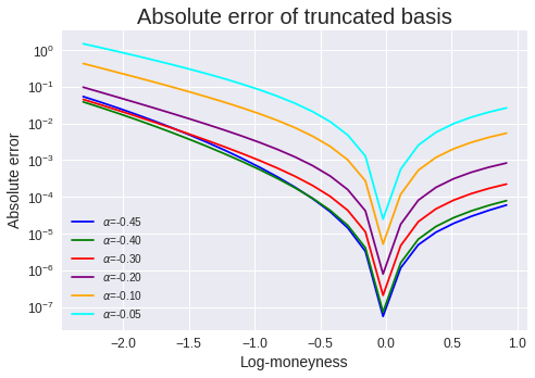
Refer to caption
Figure 11. Absolute error of the rate function. We consider the truncated basis approach against the standard polynomial basis with η=1.5\eta=1.5, v0=0.04v_{0}=0.04 and different values of α\alpha.

C.3. Multi-Factor case

The correlated mixed multi-factor rough Bergomi (2.6) model requires a slightly more complex setting. By Corollary 3.15 the rate function that we aim at is given by following multidimensional optimisation problem:

(C.4) Λ^(v,Σ)(y):=inf(f1,…,fn)∈L2​[0,1]{12∑i=1n||fi||2:y=RV(∑i=1mγiexp(νiη⋅Σi𝔣.Kα)u)(1)},\hat{\Lambda}^{(v,\Sigma)}(\mathrm{y}):=\inf_{(f_{1},...,f_{n})\in L^{2}[0,1]}\left\{\frac{1}{2}\sum_{i=1}^{n}||f_{i}||^{2}:\mathrm{y}=RV\left(\sum_{i=1}^{m}\gamma_{i}\exp\left(\frac{\nu^{i}}{\eta}\cdot\Sigma_{i}\mathfrak{f}^{K_{\alpha}}_{.}\right)u\right)(1)\right\},

where 𝔣.Kα=(∫0⋅Kα(u,⋅)f1(u)du,…,∫0⋅Kα(u,⋅)fn(u)du)\mathfrak{f}^{K_{\alpha}}_{.}=\left(\int_{0}^{\cdot}K_{\alpha}(u,\cdot)f_{1}(u)\mathrm{d}u,...,\int_{0}^{\cdot}K_{\alpha}(u,\cdot)f_{n}(u)\mathrm{d}u\right). The approach to solve this problem is similar to that of (C.1). Nevertheless, in order to solve (C.4) we shall use a multi-dimensional polynomial basis

(f^1(p)​(s),…,f^n(p)​(s))=(∑i=0pai1​si,…,∑i=0pain​si)\left(\hat{f}^{(p)}_{1}(s),...,\hat{f}^{(p)}_{n}(s)\right)=\left(\sum_{i=0}^{p}a^{1}_{i}s^{i},...,\sum_{i=0}^{p}a^{n}_{i}s^{i}\right)

such that each f^i(p)​(s)\hat{f}^{(p)}_{i}(s) for i∈{1,…,n}i\in\{1,...,n\} is dense as pp tends to +∞+\infty in L2​[0,1]L^{2}[0,1] by Stone-Weierstrass Theorem. Then we may equivalently solve

(C.5) inf(a01,…,ap1,…,a0n,…,apn)∈ℝ(p+1)​n{12∑i=1n||f^i(p)||2:y=RV(∑i=1mγiexp(νiη⋅Σi𝔣^.(Kα,p))u)(1)},\inf_{(a_{0}^{1},...,a_{p}^{1},...,a_{0}^{n},...,a_{p}^{n})\in\mathbb{R}^{(p+1)n}}\left\{\frac{1}{2}\sum_{i=1}^{n}||\hat{f}^{(p)}_{i}||^{2}:\mathrm{y}=RV\left(\sum_{i=1}^{m}\gamma_{i}\exp\left(\frac{\nu^{i}}{\eta}\cdot\Sigma_{i}\hat{\mathfrak{f}}^{(K_{\alpha},p)}_{.}\right)u\right)(1)\right\},

where 𝔣^.(Kα,p)=(∫0⋅Kα(u,⋅)f^1(p)(u)du,…,∫0⋅Kα(u,⋅)f^n(p)(u)du)\hat{\mathfrak{f}}^{(K_{\alpha},p)}_{.}=\left(\int_{0}^{\cdot}K_{\alpha}(u,\cdot)\hat{f}^{(p)}_{1}(u)\mathrm{d}u,...,\int_{0}^{\cdot}K_{\alpha}(u,\cdot)\hat{f}^{(p)}_{n}(u)\mathrm{d}u\right). Then as pp tends to +∞+\infty, (C.5) will converge to the original problem (C.4). In order to numerically accelerate the optimisation problem in (C.5), we anchor coefficients (a01,….,a0n)(a_{0}^{1},....,a_{0}^{n}) to satisfy the constraint y=R​V​(⋅)​(1)y=RV(\cdot)(1) (same way we did in the one dimensional case), that is

𝔞∗:=inf(a01,….,a0n)∈ℝn{(y−RV(∑i=1mγiexp(νiη⋅Σi𝔣.Kα)u)(1))2}\mathfrak{a}^{*}:=\inf_{(a_{0}^{1},....,a_{0}^{n})\in\mathbb{R}^{n}}\left\{\left(\mathrm{y}-RV\left(\sum_{i=1}^{m}\gamma_{i}\exp\left(\frac{\nu^{i}}{\eta}\cdot\Sigma_{i}\mathfrak{f}^{K_{\alpha}}_{.}\right)u\right)(1)\right)^{2}\right\}

where 𝔞∗=(𝔞01∗,…,𝔞0n∗)\mathfrak{a}^{*}=(\mathfrak{a}^{1*}_{0},...,\mathfrak{a}^{n*}_{0}) and one may use (C.3) and Gauss-Legendre quadrature to efficiently compute R​V​(⋅)​(1)RV(\cdot)(1). Then, the constraint will always be satisfied by construction and instead we may solve

(C.6) inf(𝔞01∗,a11…,ap1,…,𝔞0n∗,a1n,…,apn)∈ℝ(p+1)​n{12∑i=1n||f^(p)||2}.\inf_{(\mathfrak{a}_{0}^{1*},a_{1}^{1}...,a_{p}^{1},...,\mathfrak{a}_{0}^{n*},a_{1}^{n},...,a_{p}^{n})\in\mathbb{R}^{(p+1)n}}\left\{\frac{1}{2}\sum_{i=1}^{n}||\hat{f}^{(p)}||^{2}\right\}.

Appendix D Exponential Equivalence and Contraction Principle

Definition D.1.

On a metric space (𝒴,d)(\mathcal{Y},d), two 𝒴\mathcal{Y}-valued sequences (Xε)ε>0{(X^{\varepsilon})}_{\varepsilon>0} and (X~ε)ε>0{(\widetilde{X}^{\varepsilon})}_{\varepsilon>0} are called exponentially equivalent (with speed hεh_{\varepsilon}) if there exist probability spaces (Ω,ℬε,ℙε)ε>0(\Omega,\mathcal{B}_{\varepsilon},\mathbb{P}_{\varepsilon})_{\varepsilon>0} such that for any ε>0\varepsilon>0, ℙε\mathbb{P}^{\varepsilon} is the joint law of (X~ε,Xε)(\widetilde{X}^{\varepsilon},X^{\varepsilon}), ε>0\varepsilon>0 and, for each δ>0\delta>0, the set {ω:(X~ε,Xε)∈Γδ}\left\{\omega:(\widetilde{X}^{\varepsilon},X^{\varepsilon})\in\Gamma_{\delta}\right\} is ℬε\mathcal{B}_{\varepsilon}-measurable, and

lim supε↓0hε​log⁡ℙε​(Γδ)=−∞,\limsup_{\varepsilon\downarrow 0}h_{\varepsilon}\log\mathbb{P}^{\varepsilon}\left(\Gamma_{\delta}\right)=-\infty,

where Γδ:={(y~,y):d⁡(y~,y)>δ}⊂𝒴×𝒴\Gamma_{\delta}:=\left\{(\tilde{y},y):d(\tilde{y},y)>\delta\right\}\subset\mathcal{Y}\times\mathcal{Y}.

Theorem D.2.

Let 𝒳\mathcal{X} and 𝒴\mathcal{Y} be topological spaces and f:𝒳→𝒴f:\mathcal{X}\rightarrow\mathcal{Y} a continuous function. Consider a good rate function I:𝒳→[0,∞]I:\mathcal{X}\rightarrow[0,\infty]. For each y∈𝒴y\in\mathcal{Y}, define I′(y):=inf{I(x):x∈𝒳,y=f(x)}I^{\prime}(y):=\inf\{I(x):x\in\mathcal{X},y=f(x)\}. Then, if II controls the LDP associated with a family of probability measures {με}\{\mu_{\varepsilon}\} on 𝒳\mathcal{X}, the I′I^{\prime} controls the LDP associated with the family of probability measures {με∘f−1}\{\mu_{\varepsilon}\circ f^{-1}\} on 𝒴\mathcal{Y} and I′I^{\prime} is a good rate function on 𝒴\mathcal{Y}.

Appendix E Proof of v0​ϕ​(d1​(x))=x​ϕ​(d2​(x))v_{0}\phi(d_{1}(x))=x\phi(d_{2}(x))

In order to prove v0​ϕ​(d1​(x))=x​ϕ​(d2​(x))v_{0}\phi(d_{1}(x))=x\phi(d_{2}(x)), we will prove the following equivalent result

(d1​(x))2−(d2​(x))2=2​log⁡(v0x).\left(d_{1}(x)\right)^{2}-\left(d_{2}(x)\right)^{2}=2\log\left(\frac{v_{0}}{x}\right).
Proof.

Recall that ϕ⁡(⋅)\phi(\cdot) is the standard Gaussian probability density function. Using that for x≥0x\geq 0, d1​(x)=log⁡(v0)−log⁡(x)σ^​(x,T)​T+12​σ^​(x,T)​Td_{1}(x)=\frac{\log(v_{0})-\log(x)}{\hat{\sigma}(x,T)\sqrt{T}}+\frac{1}{2}\hat{\sigma}(x,T)\sqrt{T} and d2​(x)=d1​(x)−σ^​(x,T)​Td_{2}(x)=d_{1}(x)-\hat{\sigma}(x,T)\sqrt{T}, we obtain

(d1​(x))2−(d2​(x))2\displaystyle\displaystyle\left(d_{1}(x)\right)^{2}-\left(d_{2}(x)\right)^{2} =(d1​(x))2−(d1​(x)−σ^​(x,T)​T)2,\displaystyle=\left(d_{1}(x)\right)^{2}-\left(d_{1}(x)-\hat{\sigma}(x,T)\sqrt{T}\right)^{2},
=2​d1​(x)​σ^​(x,T)​T−T​σ^2​(x,T),\displaystyle=2d_{1}(x)\hat{\sigma}(x,T)\sqrt{T}-T\hat{\sigma}^{2}(x,T),
=2​[log⁡(v0)−log⁡(x)+12​σ^2​(x,T)​T]−T​σ^2​(x,T),\displaystyle=2\left[\log(v_{0})-\log(x)+\frac{1}{2}\hat{\sigma}^{2}(x,T)T\right]-T\hat{\sigma}^{2}(x,T),
=2​log⁡(v0x).\displaystyle=2\log\left(\frac{v_{0}}{x}\right).

∎

References

  • [AGM18] E. Alòs, D. García-Lorite and A. Muguruza. On smile properties of volatility derivatives and exotic products: understanding the VIX skew. arXiv:1808.03610, 2018.
  • [ALV07] E. Alòs, J. León and J. Vives. On the short-time behavior of the implied volatility for jump-diffusion models with stochastic volatility. Finance and Stochastics, 11(4), 571-589, 2007.
  • [AP18] M. Avellaneda and A. Papanicolau. Statistics of VIX Futures and Their Applications to Trading Volatility Exchange-Traded Products. The Journal of Investment Strategies, Vol. 7, No. 2, 1-33, 2018.
  • [AS72] M. Abramowitz and I.A. Stegun. Handbook of Mathematical Functions with Formulas, Graphs, and Mathematical tables. Dover, New York, 1972.
  • [AT07] R.J. Adler and J.E. Taylor. Random Fields and Geometry. Springer-Verlag, New York, 2007.
  • [Ber08] L. Bergomi. Smile dynamics III. Risk, October: 90-96, 2008.
  • [Ber16] L. Bergomi. Stochastic Volatility Modeling. Chapman & Hall/CRC financial mathematics series, 2016.
  • [BFG16] C. Bayer, P.K. Friz and J. Gatheral. Pricing under rough volatility. Quantitative Finance, 16(6): 887-904, 2016.
  • [BFGHS17] C. Bayer, P. Friz, A. Gulisashvili, B. Horvath and B. Stemper. Short-time near the money skew in rough fractional stochastic volatility models. Quantitative Finance, 17(3): 2017.
  • [BGT89] N. H. Bingham, C. M. Goldie and J. L. Teugels. Regular Variation, 2nd edition. Cambridge University Press, Cambridge, 1989.
  • [BHØZ08] F. Biagini, Y. Hu, B. Øksendal and T. Zhang. Stochastic Calculus for Fractional Brownian Motion and Applications. Springer London, 2008.
  • [BL78] D.T. Breeden and R.H. Litzenberger. Prices of state-contingent claims implicit in options prices. J. Business, 51: 621–651, 1978.
  • [BLP15] M. Bennedsen, A. Lunde and M.S. Pakkanen. Hybrid scheme for Brownian semistationary processes. Finance and Stochastics, 21(4): 931-965, 2017.
  • [BS07] O. E. Barndorff-Nielsen and J. Schmiegel. Ambit processes: with applications to turbulence and tumour growth. In F. E. Benth, G. Di Nunno, T. Lindstrøm, B. Øksendal and T. Zhang (Eds.), 2007. Stochastic analysis and applications, volume 2 of Abel Symp.: 93-124, Springer, Berlin.
  • [CGMY05] P. Carr, H. Geman, D. Madan, and M. Yor. Pricing options on realized variance. Finance and Stochastics, 9(4):453–475, 2005.
  • [Che08] A. Cherny. Brownian moving averages have conditional full support. Ann. App. Prob., 18(5): 1825-1850, 2008.
  • [CL09] P. Carr and R. Lee. Volatility Derivatives. Annual Review of Financial Economics 1(1), 319-339,2009.
  • [DS89] J.D. Deuschel and D.W. Stroock. Large Deviations. Academic Press, Boston, 1989.
  • [DZ10] A. Dembo and O. Zeitouni. Large Deviations Theory and Applications, Second Edition. Springer-Verlag Berlin Heidelberg, 2010.
  • [ER18] O. El Euch and M. Rosenbaum. Perfect hedging under rough Heston models. The Annals of Applied Probability, 28 (6): 3813-3856, 2018.
  • [ER19] O. El Euch and M. Rosenbaum. The characteristic function of rough Heston models. Mathematical Finance, 29 (1): 3-38, 2019.
  • [FGP18] P. Friz, P. Gassiat and P. Pigato. Precise asymptotics: robust stochastic volatility models. Preprint available at arXiv:1811.00267, 2018.
  • [FZ17] M. Forde and H. Zhang. Asymptotics for rough stochastic volatility models. SIAM J. Finan. Math., 8(1): 114-145, 2017.
  • [Gas18] P. Gassiat. On the martingale property in the rough Bergomi model. Electron. Commun. Probab. 24(33), 2019.
  • [GJR18] J. Gatheral, T. Jaisson and M. Rosenbaum. Volatility is rough. Quantitative Finance, 18(6): 933-949, 2018.
  • [GL14] K. Gao and R. Lee. Asymptotics of implied volatility to arbitrary order. Finance and Stochastics, 18(2): 349-392, 2014.
  • [HJL18] B. Horvath, A. Jacquier, and C. Lacombe. Asymptotic behaviour of randomised fractional volatility models. Forthcoming Journal of Applied Probability, 2019.
  • [HJM17] B. Horvath, A. Jacquier and A. Muguruza. Functional central limit theorems for rough volatility. arXiv:1711.03078, 2017.
  • [HJT18] B. Horvath, A. Jacquier and P. Tankov. Volatility options in rough volatility models. SIAM J. Finan. Math., 11(2): 437-469, 2020
  • [HMT19] B. Horvath, A. Muguruza and M. Tomas. Deep Learning Volatility. arXiv:1901.09647, 2019.
  • [JMM18] A. Jacquier, C. Martini, A. Muguruza. On VIX Futures in the rough Bergomi model. Quant. Finance, 18(1): 45-61, 2018.
  • [JPS18] A. Jacquier, M. Pakkanen, and H. Stone. Pathwise Large Deviations for the rough Bergomi model. Journal of Applied Probability 55(4): 1078-1092, 2018.
  • [MP18] R. McCrickerd and M. Pakkanen. Turbocharging Monte Carlo pricing for the rough Bergomi model Quant. Finance, 18(11): 1877–1886, 2018.
  • [Neu94] A. Neuberger. The log contract. Journal of Portfolio Management, 20(2): 74-80, 1994.
  • [PZ16] D. Pirjol and L. Zhu. Short Maturity Asian Options in Local Volatility Models.SIAM Journal on Financial Mathematics,7: 947-992,2016.
  • [Sto19] H. Stone. Calibrating rough volatility models: a convolutional neural network approach. Quantitative Finance, 20(3): 379-392, 2020.