A fast, low-leakage, high-fidelity two-qubit gate for a programmable superconducting quantum computer
Abstract
A common approach to realize conditional-phase (CZ) gates in transmon qubits relies on flux control of the qubit frequency to make computational states interact with non-computational ones using a fast-adiabatic trajectory to minimize leakage. We develop a bipolar flux-pulsing method with two key advantages over the traditional unipolar variant. First, the action of the bipolar pulse is robust to long-timescale linear-dynamical distortions in the flux-control line, facilitating tuneup and ensuring atomic repeatability. Second, the flux symmetry of the transmon Hamiltonian makes the conditional phase and the single-qubit phase of the pulsed qubit first-order insensitive to low-frequency flux noise, increasing fidelity. By harnessing destructive interference to minimize leakage, the bipolar pulse can approach the speed limit set by the exchange coupling. We demonstrate a repeatable, high-fidelity (), low-leakage (), and fast () CZ gate in a circuit QED quantum processor. Detailed numerical simulations with excellent match to experiment show that leakage is dominated by remaining short-timescale distortions and fidelity is limited by high-frequency flux noise.
A steady increase in qubit counts Otterbach et al. 2017; Knight; Kelly; Intel and operation fidelities Barends et al. 2014; Rol et al. 2017; Hong et al. 2019; Sheldon et al. 2016; Heinsoo et al. 2018 allows quantum computing platforms using monolithic superconducting quantum hardware to target outstanding challenges such as quantum advantage Boixo et al. 2018; Neill et al. 2018; Bravyi et al. 2018, quantum error correction (QEC) Kelly et al. 2015; Ristè et al. 2015; Takita et al. 2016; Bultink et al. 2019; Andersen et al. 2019, and quantum fault tolerance (QFT) Fowler et al. 2012; Martinis 2015. All of these pursuits require two-qubit gates with fidelities exceeding , fueling very active research.
There are three main types of two-qubit gates in use for transmon qubits, all of which harness exchange interactions between computational states () or between computational and non-computational states ( or ), mediated by a coupling bus or capacitor. Cross-resonance gates Chow et al. 2011; Sheldon et al. 2016 exploit the exchange interaction between and using microwave-frequency transversal drives. Parametric gates Caldwell et al. 2018; Hong et al. 2019 employ radio-frequency longitudinal drives, specifically flux pulses modulating the qubit frequency, to generate sidebands of resonance between and for iSWAP or between and or for conditional-phase (CZ). The oldest approach Strauch et al. 2003; DiCarlo et al. 2009 uses baseband flux pulses to tune into near resonance with to realize CZ. Either because they explicitly use non-computational states, or because of frequency crowding and the weak transmon anharmonicity, the three approaches are vulnerable to leakage of information from the computational space. Leakage is very problematic in applications such as QEC, complicating the design of error decoders and/or demanding operational overhead to generate seepage Aliferis and Terhal 2007; Ghosh et al. 2013; Fowler 2013; Suchara et al. 2015; Ghosh and Fowler 2015, generally reducing the error thresholds for QFT. This threat has motivated the design of fast-adiabatic pulsing methods Martinis and Geller 2014 to mitigate leakage and architectural choices in qubit frequency and coupler arrangements Versluis et al. 2017 to explicitly avoid it. Surprisingly, many recent demonstrations Sheldon et al. 2016; Wang et al. 2018; Hong et al. 2019 of two-qubit gates place emphasis on reaching or approaching fidelity without separately quantifying leakage.
Although baseband flux pulsing produces the fastest two-qubit gates to date (), two challenges have kept it from becoming the de facto two-qubit gating method. First, because the pulse displaces one qubit below its flux-symmetry point, i.e., the sweetspot, the temporary first-order sensitivity to flux noise increases dephasing and impacts fidelity. The second challenge is non-atomicity. If uncompensated, linear-dynamical distortions in the flux-control lines originating from limited waveform-generator bandwidth, high-pass bias tees, low-pass filters, impedance mismatches, on-chip response, etc., can make the action of a pulse depend on the detailed history of flux pulses applied. To date, predistortion corrections have been calculated in advance, requiring prior knowledge of the timing of all the flux-pulse-based operations required by the quantum circuit, and significant waveform memory. This standard practice is incompatible with real-time determination and execution of operations, as is required for control flow and feedback in a fully programmable quantum computer Fu et al. 2017; Fu et al. 2019.
In this Letter, we introduce a fast (), low-leakage (), high-fidelity (), and repeatable flux-pulse-based gate suitable for a full-stack quantum computer executing operations in real time on transmon-based quantum hardware. These attractive characteristics are enabled by a zero-average bipolar flux-pulsing method, nicknamed Net-Zero (NZ), which uses the avoided crossing twice. Harnessing the analogy to a Mach-Zehnder interferometer, NZ exploits destructive interference to minimize leakage to while approaching the speed limit set by the exchange coupling in the two-excitation manifold. The flux symmetry of the transmon Hamiltonian makes the conditional phase and the single-qubit phase acquired by the pulsed qubit first-order insensitive to low-frequency flux noise, increasing fidelity relative to a unipolar pulse. Crucially, the zero-average characteristic makes NZ insensitive to long timescale linear-dynamical distortions remaining in the flux-control line after best efforts at real-time pre-compensation, making the gate repeatable. Detailed numerical simulations supplied with calibrated experimental parameters and direct measurement of remaining short-timescale distortions show an excellent match to experiment, and indicate that fidelity is limited by high-frequency flux noise while leakage is dominated by the remaining short-timescale distortions.

The ideal gate is described by the transformation:
| (1) |
in the computational basis , where the single-qubit phases and are even multiples of and the conditional phase defined by is an odd multiple of . A gate of total duration can be realized in two steps. First, a strong flux pulse on the higher frequency qubit moves into the avoided crossing with and back to acquire . Next, simultaneous weaker pulses on both qubits adjust the single-qubit phases. We compare two types of flux pulses, the (unipolar) pulse introduced in Martinis and Geller 2014 and the pulse [Fig. 1(a)]. The pulse consists of two back-to-back unipolar pulses of half the duration and opposite amplitude. Experiments are performed on a pair of flux-tunable transmons described in more detail in the Supplemental Material Sup.
Because of distortions, the waveform specified in an arbitrary waveform generator (AWG) does not result in the qubit experiencing the targeted flux . These distortions can be described as a linear time-invariant system that transduces voltage to flux and is characterized by its impulse response . It is possible to measure at the qubit using our Cryoscope technique Rol et al. 2019 and construct an inverse filter to correct for distortions. By performing a convolution of the desired signal with , known as a predistortion correction, the qubit experiences the pulse
| (2) |
The predistortion corrections are performed using a combination of real-time filters implemented in a Zurich Instruments HDAWG and a short () FIR filter implemented off line.
By eliminating the DC component of the pulse, gates are resilient to remaining long-timescale distortions Johnson 2011. Because the transmon Hamiltonian is symmetric with respect to the sweetspot, it is possible to use both positive and negative amplitudes to perform a gate [Fig. 1(b)] while also satisfying the zero-average condition
| (3) |
If Eq. 3 holds, the DC component is zero and the components in the Fourier transform at frequencies are suppressed. Writing Eq. 2 in the Fourier domain: , it follows that if does not contain any components at , then does not depend on any components of at frequencies . As a consequence, the required corrections for pulses do not accumulate, eliminating the need for accurate long-timescale distortion corrections and the resulting history-dependent errors [Fig. 1(d)].

To measure the repeatability of gates, the phase () acquired by the pulsed qubit during a gate is measured as a function of the separation time to an earlier gate (Fig. 2). Because of the detuning from the sweetspot, a small change in amplitude during the pulse leads to a significant change in frequency. This makes the phase acquired during the pulse very sensitive to distortions. We observe that not correcting distortions leads to significant phase errors (). Correcting distortions using a predistortion filter keeps the error small () for the first but shows clear history-dependent behavior for longer timescales. Using pulses in combination with a predistortion filter eliminates all history dependence. Hence, we conclude that pulses are robust against remaining long-timescale distortions.

We next investigate a built-in echo effect that provides protection against flux noise. Because the derivative of the flux arc is equal and opposite in sign at the positive and negative halves of the pulse, we expect and to be first-order insensitive to low-frequency flux noise. As a test, we measure the dependence of on an applied DC flux offset for both a unipolar and gate [Fig. 3]. As shown in Fig. 3(b), is first-order sensitive for a unipolar pulse and only second-order sensitive for . We have also measured how the dephasing time depends on the detuning for both a square flux pulse and two half-square flux pulses with opposite sign Sup. We find that the dephasing rate is significantly reduced when the opposite-sign flux pulses are used, confirming that pulses have a built-in echo effect.
The pulse shape is intended to minimize leakage and is described by two parameters Sup. Parameter is a measure of the flux at the middle of the unipolar pulse, and at the middle of each half of . States and are resonant at . Parameter tunes the sharpness of the pulse rise and fall. We follow Wood and Gambetta 2018 in defining the leakage () of an operation as the average probability that a random computational state leaks out of the computational subspace.
In order to gain insight into how and depend on the pulse shape, we perform an experiment and compare this to simulations. The conditional oscillation experiment (Fig. 4) consists of a Ramsey-like experiment that allows us to measure and estimate . This experiment measures the phase acquired during an (uncalibrated) CZ gate by the target qubit () while either leaving the control qubit () in the ground state, or adding and subsequently removing an excitation to . The difference between the phase acquired when is in and when is in gives . If leakage from to occurs, is in when the second pulse, intended to remove the excitation, is applied. This will result in adding, instead of removing, an excitation to . The leakage probability can be estimated as , where is the population difference on the control qubit between both variants of the experiment. Because of relaxation effects, slightly overestimates .
The simulations model the system in a realistic way and allow us to extract , and the average gate fidelity for a single application of the gate Sup. The pulse is modeled as a trajectory in a two-qutrit Hamiltonian. The noise model accounts for relaxation and dephasing effects as well as the effect of the calibrated remaining distortions. For the dephasing we take into account the different timescales on which flux noise acts as well as their dependence on the flux bias. Distortions are modeled based on the remaining distortions measured using the Cryoscope technique Rol et al. 2019.

Both the experiment and simulation show a fringe of low leakage [Fig. 4(b,d)]. This fringe can be understood by analogy to a Mach-Zehnder interferometer Sup. The states and correspond to two paths of the interferometer. The first part of the pulse (red in Fig. 1) corresponds to the first (imbalanced) beamsplitter of the interferometer. In general, after the first beamsplitter most of the population remains in but a small part is transferred to . Pulsing through the sweetspot (green in Fig. 1) corresponds to the arms of the interferometer. The two paths are detuned by , causing a phase to be acquired before the paths are recombined at the second half of the pulse (blue in Fig. 1) corresponding to the second beamsplitter. The phase difference between the two paths will cause interference that either enhances or suppresses the leakage to Sup.
Given the good correspondence between experiment and simulation (Fig. 4), we can use simulations to explore the parameter space to find the shortest and corresponding parameters enabling a high-fidelity, low-leakage gate. The minimum gate duration is fundamentally limited by the coupling strength as the time required to acquire 180 degrees of conditional phase at the avoided crossing: . We find a pulse that makes use of the Mach-Zehnder interference condition to achieve a low leakage. We append a ns flux pulse to correct the single-qubit phases on both qubits, making the total duration of the phase-corrected gate ns. We ensure that these phase-correction pulses satisfy Eq. 3 and have a sufficiently low amplitude to not affect and significantly.
We characterize the performance of the gate using an interleaved randomized benchmarking protocol Magesan et al. 2012; Barends et al. 2014 with a few modifications that allow us to quantify leakage Asaad et al. 2016; Wood and Gambetta 2018; Sup. The randomized benchmarking sequences are based on 300 random seeds. For each seed, every data point is measured 104 times. We measure an average gate fidelity and leakage for the pulse with [Fig. 5(a,b)]. We did not perform similar measurements for the unipolar pulse as this gate is not repeatable.
It is possible to investigate the limits to the performance of the gate using simulation. We simulate this gate for a range of different error models [Fig. 5(c,d)]. A first observation is that the infidelity () of the gate does not significantly increase when the low-frequency flux-noise components are included in the simulations, whereas this does affect the unipolar pulse. It appears that the difference in between the unipolar and pulses for the full model including distortions can be attributed completely to this effect. This observation is consistent with the echo effect demonstrated in Fig. 3. Looking at the error budgets, is limited by distortions. This is understandable as minimizing requires the pulse to follow a precise trajectory. The simulations also indicate that dephasing causes leakage. This can be understood as dephasing effectively corresponds to an uncertainty in the energy of these levels. The simulated is larger than the measured . This could be explained in two ways, either the distortions are less severe than our estimate, or the simulations, only concerned with a single application of the gate, do not take into account all the relevant effects. Specifically, because the population in the leakage subspace does not completely decohere, this population can seep back into the computational subspace due to an interference effect (similar to that in the pulse itself) at subsequent applications of the gate. Because the first gate cannot benefit from this coherence, the simulations, which only deal with a single gate, slightly overestimate the effective leakage.

In summary, we have demonstrated a flux-based gate for transmon qubits that is fast, low-leakage, high-fidelity and repeatable. The gate is realized using a bipolar Net-Zero flux pulse that harnesses a Mach-Zehnder-like interference to achieve speed while reducing leakage by destructive interference. The NZ pulse exploits the flux symmetry of the pulsed transmon to build in an echo effect on its single-qubit phase and the conditional phase, increasing fidelity relative to a unipolar pulse. Finally, the action of the NZ pulse is robust to long-timescale distortions in the flux-control line remaining after real-time pre-compensation, enabling the repeatability of the gate. These features make the realized NZ CZ gate immediately useful in high-circuit-depth applications of a full-stack quantum computer in which a controller issues operations to execute on the quantum hardware in real time. For example, current work in our group uses NZ CZ gates to stabilize two-qubit entanglement by multi-round indirect parity measurements Bultink et al. 2019. Future work will incorporate NZ CZ gates into our scheme Versluis et al. 2017 to realize a surface-code-based logical qubit Fowler et al. 2012 with monolithic transmon-cQED quantum hardware.
Acknowledgements.
We thank J. Helsen, T. O’Brien, X. Bonet-Monroig, N. Haandaek, Y. Salathe, and V. Ostroukh for useful discussions. This research is supported by the Office of the Director of National Intelligence (ODNI), Intelligence Advanced Research Projects Activity (IARPA), via the U.S. Army Research Office grant W911NF-16-1-0071. The views and conclusions contained herein are those of the authors and should not be interpreted as necessarily representing the official policies or endorsements, either expressed or implied, of the ODNI, IARPA, or the U.S. Government. F.B. and B.M.T. are supported by ERC grant EQEC No. 682726.References
- Otterbach et al. (2017) J. S. Otterbach, R. Manenti, N. Alidoust, A. Bestwick, M. Block, B. Bloom, S. Caldwell, N. Didier, E. Schuyler Fried, S. Hong, P. Karalekas, C. B. Osborn, A. Papageorge, E. C. Peterson, G. Prawiroatmodjo, N. Rubin, C. A. Ryan, D. Scarabelli, M. Scheer, E. A. Sete, P. Sivarajah, R. S. Smith, A. Staley, N. Tezak, W. J. Zeng, A. Hudson, B. R. Johnson, M. Reagor, M. P. da Silva, and C. Rigetti, arXiv:1712.05771 (2017).
- (2) W. Knight, “IBM raises the bar with a 50-qubit quantum computer,” https://www.technologyreview.com/s/609451/ibm-raises-the-bar-with-a-50-qubit-quantum-computer/.
- (3) J. Kelly, “A preview of Bristlecone, Google’s new quantum processor,” https://ai.googleblog.com/2018/03/a-preview-of-bristlecone-googles-new.html.
- (4) Intel, “The future of quantum computing is counted in qubits,” https://newsroom.intel.com/news/future-quantum-computing-counted-qubits/.
- Barends et al. (2014) R. Barends, J. Kelly, A. Megrant, A. Veitia, D. Sank, E. Jeffrey, T. C. White, J. Mutus, A. G. Fowler, B. Campbell, Y. Chen, Z. Chen, B. Chiaro, A. Dunsworth, C. Neill, P. O’Malley, P. Roushan, A. Vainsencher, J. Wenner, A. N. Korotkov, A. N. Cleland, and J. M. Martinis, Nature 508, 500 (2014).
- Rol et al. (2017) M. A. Rol, C. C. Bultink, T. E. O’Brien, S. R. de Jong, L. S. Theis, X. Fu, F. Luthi, R. F. L. Vermeulen, J. C. de Sterke, A. Bruno, D. Deurloo, R. N. Schouten, F. K. Wilhelm, and L. DiCarlo, Phys. Rev. Applied 7, 041001 (2017).
- Hong et al. (2019) S. S. Hong, A. T. Papageorge, P. Sivarajah, G. Crossman, N. Dider, A. M. Polloreno, E. A. Sete, S. W. Turkowski, M. P. da Silva, and B. R. Johnson, ArXiv:1901.08035 (2019).
- Sheldon et al. (2016) S. Sheldon, E. Magesan, J. M. Chow, and J. M. Gambetta, Physical Review A 93, 060302 (2016).
- Heinsoo et al. (2018) J. Heinsoo, C. K. Andersen, A. Remm, S. Krinner, T. Walter, Y. Salathé, S. Gasparinetti, J.-C. Besse, A. Potočnik, A. Wallraff, and C. Eichler, Phys. Rev. Applied 10, 034040 (2018).
- Boixo et al. (2018) S. Boixo, S. V. Isakov, V. N. Smelyanskiy, R. Babbush, N. Ding, Z. Jiang, M. J. Bremner, J. M. Martinis, and H. Neven, Nature Physics 14, 595 (2018).
- Neill et al. (2018) C. Neill, P. Roushan, K. Kechedzhi, S. Boixo, S. V. Isakov, V. Smelyanskiy, A. Megrant, B. Chiaro, A. Dunsworth, K. Arya, R. Barends, B. Burkett, Y. Chen, Z. Chen, A. Fowler, B. Foxen, M. Giustina, R. Graff, E. Jeffrey, T. Huang, J. Kelly, P. Klimov, E. Lucero, J. Mutus, M. Neeley, C. Quintana, D. Sank, A. Vainsencher, J. Wenner, T. C. White, H. Neven, and J. M. Martinis, Science 360, 195 (2018).
- Bravyi et al. (2018) S. Bravyi, D. Gosset, and R. König, Science 362, 308 (2018).
- Kelly et al. (2015) J. Kelly, R. Barends, A. Fowler, A. Megrant, E. Jeffrey, T. White, D. Sank, J. Mutus, B. Campbell, Y. Chen, et al., Nature 519, 66 (2015).
- Ristè et al. (2015) D. Ristè, S. Poletto, M. Z. Huang, A. Bruno, V. Vesterinen, O. P. Saira, and L. DiCarlo, Nat. Commun. 6, 6983 (2015).
- Takita et al. (2016) M. Takita, A. D. Córcoles, E. Magesan, B. Abdo, M. Brink, A. Cross, J. M. Chow, and J. M. Gambetta, arXiv:1605.01351 (2016).
- Bultink et al. (2019) C. C. Bultink, R. Vollmer, T. E. O’Brien, N. Muthusubramanian, M. Beekman, M. A. Rol, B. Tarasinski, and L. DiCarlo, In preparation (2019).
- Andersen et al. (2019) C. Andersen, A. Remm, S. Balasiu, S. Krinner, J. Heinsoo, J. Besse, M. Gabureac, A. Wallraff, and C. Eichler, arXiv:1902.06946 (2019).
- Fowler et al. (2012) A. G. Fowler, M. Mariantoni, J. M. Martinis, and A. N. Cleland, Phys. Rev. A 86, 032324 (2012).
- Martinis (2015) J. M. Martinis, npj Quantum Inf. 1, 15005 (2015).
- Chow et al. (2011) J. M. Chow, A. D. Córcoles, J. M. Gambetta, C. Rigetti, B. R. Johnson, J. A. Smolin, J. R. Rozen, G. A. Keefe, M. B. Rothwell, M. B. Ketchen, and M. Steffen, Phys. Rev. Lett. 107, 080502 (2011).
- Caldwell et al. (2018) S. A. Caldwell, N. Didier, C. A. Ryan, E. A. Sete, A. Hudson, P. Karalekas, R. Manenti, M. P. da Silva, R. Sinclair, E. Acala, N. Alidoust, J. Angeles, A. Bestwick, M. Block, B. Bloom, A. Bradley, C. Bui, L. Capelluto, R. Chilcott, J. Cordova, G. Crossman, M. Curtis, S. Deshpande, T. E. Bouayadi, D. Girshovich, S. Hong, K. Kuang, M. Lenihan, T. Manning, A. Marchenkov, J. Marshall, R. Maydra, Y. Mohan, W. O’Brien, C. Osborn, J. Otterbach, A. Papageorge, J.-P. Paquette, M. Pelstring, A. Polloreno, G. Prawiroatmodjo, V. Rawat, M. Reagor, R. Renzas, N. Rubin, D. Russell, M. Rust, D. Scarabelli, M. Scheer, M. Selvanayagam, R. Smith, A. Staley, M. Suska, N. Tezak, D. C. Thompson, T.-W. To, M. Vahidpour, N. Vodrahalli, T. Whyland, K. Yadav, W. Zeng, and C. Rigetti, Phys. Rev. Applied 10, 034050 (2018).
- Strauch et al. (2003) F. W. Strauch, P. R. Johnson, A. J. Dragt, C. J. Lobb, J. R. Anderson, and F. C. Wellstood, Phys. Rev. Lett. 91, 167005 (2003).
- DiCarlo et al. (2009) L. DiCarlo, J. M. Chow, J. M. Gambetta, L. S. Bishop, B. R. Johnson, D. I. Schuster, J. Majer, A. Blais, L. Frunzio, S. M. Girvin, and R. J. Schoelkopf, Nature 460, 240 (2009).
- Aliferis and Terhal (2007) P. Aliferis and B. M. Terhal, Quantum Info. Comput. 7, 139 (2007).
- Ghosh et al. (2013) J. Ghosh, A. G. Fowler, J. M. Martinis, and M. R. Geller, Phys. Rev. A 88, 062329 (2013).
- Fowler (2013) A. G. Fowler, Phys. Rev. A 88, 042308 (2013).
- Suchara et al. (2015) M. Suchara, A. W. Cross, and J. M. Gambetta, Quantum Info. Comput. 15, 997 (2015).
- Ghosh and Fowler (2015) J. Ghosh and A. G. Fowler, Phys. Rev. A 91, 020302 (2015).
- Martinis and Geller (2014) J. M. Martinis and M. R. Geller, Phys. Rev. A 90, 022307 (2014).
- Versluis et al. (2017) R. Versluis, S. Poletto, N. Khammassi, B. Tarasinski, N. Haider, D. J. Michalak, A. Bruno, K. Bertels, and L. DiCarlo, Phys. Rev. Appl. 8, 034021 (2017).
- Wang et al. (2018) Y. Wang, Y. Li, Z. Yin, and B. Zeng, npj Quantum Inf. 4, 46 (2018).
- Fu et al. (2017) X. Fu, M. A. Rol, C. C. Bultink, J. van Someren, N. Khammassi, I. Ashraf, R. F. L. Vermeulen, J. C. de Sterke, W. J. Vlothuizen, R. N. Schouten, C. G. Almudever, L. DiCarlo, and K. Bertels, in Proceedings of the 50th Annual IEEE/ACM International Symposium on Microarchitecture, MICRO-50 ’17 (ACM, New York, NY, USA, 2017) pp. 813–825.
- Fu et al. (2019) X. Fu, L. Riesebos, M. A. Rol, J. van Straten, J. van Someren, N. Khammassi, I. Ashraf, R. F. L. Vermeulen, V. Newsum, K. K. L. Loh, J. C. de Sterke, W. J. Vlothuizen, R. N. Schouten, C. G. Almudever, L. DiCarlo, and K. Bertels, in Proceedings of 25th IEEE International Symposium on High-Performance Computer Architecture (HPCA) (IEEE, 2019) pp. 224–237.
- (34) See supplemental material.
- Rol et al. (2019) M. A. Rol, F. K. Malinowski, L. S. Ciorciaro, B. Tarasinski, Y. Salathe, N. Haandbaek, J. Sedivy, C. C. Bultink, and L. DiCarlo, In preparation (2019).
- Johnson (2011) B. R. Johnson, Controlling Photons in Superconducting Electrical Circuits, PhD Dissertation, Yale University (2011).
- Wood and Gambetta (2018) C. J. Wood and J. M. Gambetta, Phys. Rev. A 97, 032306 (2018).
- Magesan et al. (2012) E. Magesan, J. M. Gambetta, B. R. Johnson, C. A. Ryan, J. M. Chow, S. T. Merkel, M. P. da Silva, G. A. Keefe, M. B. Rothwell, T. A. Ohki, M. B. Ketchen, and M. Steffen, Phys. Rev. Lett. 109, 080505 (2012).
- Asaad et al. (2016) S. Asaad, C. Dickel, S. Poletto, A. Bruno, N. K. Langford, M. A. Rol, D. Deurloo, and L. DiCarlo, npj Quantum Inf. 2, 16029 (2016).
Supplemental material for “A fast, low-leakage, high-fidelity two-qubit gate for a programmable superconducting quantum computer”
August 11, 2026
This supplemental material contains detailed information on the experimental protocols and the simulations performed in this work. Section .1 provides relevant device parameters. Section .2 describes the parametrization used for the unipolar and pulses. Section .3 describes the simulations in detail. Section .4 and Section .7 describe protocols used to characterize the flux pulses. Section .5 investigates the limitations of the gate. Section .6 discusses the Mach-Zehnder interferometer analogy in detail.
.1 Device parameters
All experiments were performed on a circuit-QED quantum chip containing three starmon-type Versluis et al. 2017 transmon qubits, labeled , , and . Pairs - and - are coupled by separate bus resonators. Each qubit has a microwave drive line for single-qubit gating, a flux-bias line for local and ns-timescale control of the qubit frequency, and dedicated, fast readout resonators with Purcell protection for the qubits. The readout resonators are coupled to a common feed line, allowing independent readout of the three qubits by frequency multiplexing.
In this work we focus on the transmon pair -. We have achieved similar performance (fidelity, leakage and gate time) for the pair -. Relevant device parameters are given in Table S1.
| Parameter | ||||
|---|---|---|---|---|
| operating point (GHz) | 5.02 | 5.79 | 6.87 | |
| sweetspot (GHz) | 5.02 | 5.79 | 6.91 | |
| (MHz) | -300 | -300 | -331 | |
| avoided crossing (MHz) | 17.2 | 14.3 | ||
| 31.8 | 15.2 | 19.2 | ||
| operating point | 14.0 | 14.8 | 3.2 | |
| operating point | 33.8 | 19.4 | 14.7 | |
| (GHz) | 8.5 | 8.5 | ||
.2 Flux pulse parametrization
Unipolar and pulses are based on the Martinis-Geller parametrization for fast-adiabatic gates Martinis and Geller 2014. This parametrization is determined by the Hamiltonian [Eq. S8] projected onto a two-dimensional subspace. In the case of the gate, this subspace is spanned by the states and . The projected Hamiltonian, , takes the form
| (S1) |
where is the bare detuning between and and is their coupling. The detuning is controlled by flux whereas is considered to be constant. We define the angle as
| (S2) |
Note that at .
The waveform is expressed as a series
| (S3) |
where is the pulse duration, corresponds to the detuning at the operating point and is proper time, which is related to real time through .
We truncate the series to . We make use of the relation between the angle at the middle of the unipolar pulse () and the odd coefficients
| (S4) |
to define the entire waveform using three parameters: , and . A pulse is a sequence of two concatenated unipolar pulses, each lasting time and with the same and .
There are a few more transformations required in order to have a waveform in terms of the flux [Fig. S1]:
| (S5) |
The first transformation uses Eq. S2: . The second one uses the fact that by definition . The qubit frequency depends on flux according to the formula
| (S6) |
where is the sweetspot frequency and the anharmonicity, reported in Table S1. We refer to this relation between frequency and flux as the flux arc. The flux arc has been measured in the experiment and we find that it matches well with Eq. S6. We invert Eq. S6 to convert . Since , there is a positive and a negative solution for every value of . In the case of a unipolar pulse, we always consider the positive solution, whereas, in the case of a pulse, the first and second half of the pulse use the positive and negative solutions, respectively. Changes that are clearly visible in the parametrization correspond to only a small change in the applied flux. This provides intuition why even a small distortion of the applied flux can have a relatively large effect on the gate quality.

.3 Simulation structure
The simulations model the system, consisting of two coupled transmons, using a two-qutrit Hamiltonian. One of the two transmons, namely , is actively pulsed into resonance according to the pulse parametrization described in Section .2. The simulations (Fig. S2) include distortions, relaxation and flux-dependent dephasing effects. The error model also includes a distinction between Markovian (fast) and non-Markovian (slow) noise in order to accurately model dephasing effects. The simulations are used to calculate the propagator or time-evolution superoperator, from which the quantities of interest - fidelity, leakage and conditional phase - are extracted.
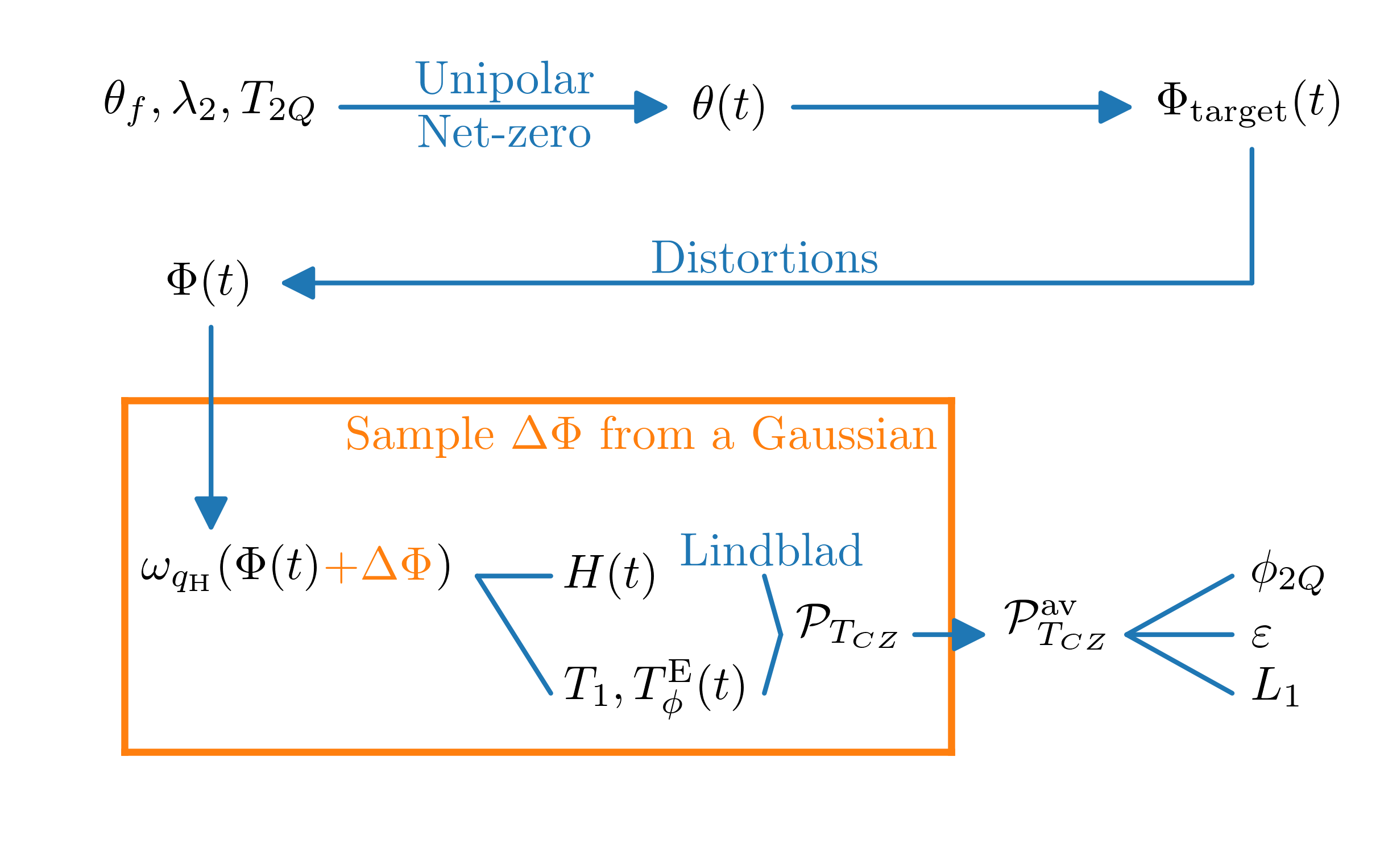
.3.1 System Hamiltonian
The system is composed of two transmons coupled via a bus resonator. We exclude the resonator from the model by making the assumption that it always remains in its ground state (it is excited only “virtually”). We restrict each transmon to its first three energy levels. In the dispersive regime, in the rotating-wave approximation, the Hamiltonian is given by
| (S7) | ||||
| (S8) |
where only the higher-frequency transmon () is actively fluxed. Here is the annihilation operator restricted to the first three energy levels, and are the qubit frequency and anharmonicity respectively, and is the coupling. The coupling is weakly flux-dependent since , with the coupling of to the bus resonator and given the parameters in Table S1. When we generate the flux pulse according to Section .2, we consider to be constant and equal to its measured value at the avoided crossing, whereas in the simulations we take into account the dependence of and on .
.3.2 Distortions
The flux pulse at the qubit is subject to distortions altering the shape of the waveform as experienced by the qubit. Distortions are described as a linear time-invariant system fully characterized by the impulse response of the system. We best compensate such distortions by predistorting the desired pulse with an impulse response designed to invert . Then, the actual pulse experienced by the qubit is given by
| (S9) |
where denotes convolution. The distortions remaining after applying are determined by measuring the step response (Fig. S3) using the Cryoscope technique Rol et al. 2019. The impulse response extracted from this data is used to distort the pulses in simulations.

.3.3 Noise model
There are two major error sources in superconducting qubits: relaxation and flux noise. The latter has a power spectral density , where is frequency and is a constant of the order of 10 , with the flux quantum. contains both high-frequency and low-frequency components: we phenomenologically distinguish high and low frequencies depending on whether they are larger or smaller than . Relaxation and high-frequency flux-noise components are Markovian noise processes since they act on a timescale shorter than the gate time. On the other hand, the low-frequency flux-noise components determine a non-Markovian noise process, since they induce correlations across different gates.
We perform two experiments to quantify the strength of the dephasing affecting : a Ram-Z and an Echo-Z experiment [Fig. S4]. In these experiments, the dephasing times and , respectively, at different flux sensitivities are measured while applying a flux pulse. In the Ram-Z experiment, this flux pulse is square. In the Echo-Z experiment, the flux pulse consists of two square half pulses that detune the qubit by the same amount in magnitude but with opposite-sign sensitivity. We perform these experiments for a range of fluxes. The experimental data for is represented in Fig. S4. On the other hand, the static qubit is always operated at the sweetspot. Therefore, we only use the measured Ramsey and Echo dephasing times at the sweetspot Table S1. The relaxation times and , are also reported in Table S1.
We assume that the low-frequency flux-noise components are echoed out in an Echo-Z experiment. In other words, we assume that , quantify the strength of the Markovian noise. On the other hand, we assume that , quantify the strength of the overall noise (both Markovian and non-Markovian). The strength of the non-Markovian noise alone cannot be extracted directly from the experiment. However, in the following we explain the model that we use fitting the experimental data (Fig. S4). In this way we can simulate separately both the Markovian and non-Markovian noise, and obtain a realistic simulation of the system.
Model of Markovian noise.
A Markovian evolution is modeled with the Lindblad equation
| (S10) |
where is the time-dependent Lindbladian defined by the Hamiltonian [Eq. S8] and by the jump operators specified in Eqs. S11, S13, S14 and S15 below.
To model relaxation, we use the jump operator
| (S11) |
To model pure dephasing, we first define a pure-dephasing time
| (S12) |
Ignoring relaxation-induced dephasing in this paragraph, the coherence decays as , where is the qutrit reduced density matrix. In Fig. S4 we see that the decay rates have a linear dependence on the flux sensitivity. Ignoring the anharmonicity, the frequency of the state is twice the frequency of the state, therefore, the sensitivity of the state is twice as high. Given these two observations, we assume that and . We find that such decay rates can be realized by the following jump operators
| (S13) | ||||
| (S14) | ||||
| (S15) |
Instead, if one would use only
| (S16) |
which produces the same Lindbladian as , then one would get and . This means that Eq. S16 would be the correct modeling if the decay rates in Fig. S4 would depend quadratically on the sensitivity, but they do not.
The formal solution of Eq. S10 is given by
| (S17) |
where is the time-ordering operator. We call the propagator or time-evolution superoperator, evaluated up to the gate time , which includes an idling time to account for the noise during the single-qubit phase correction pulses. The propagator can be computed by solving the differential Eq. S10, or as
| (S18) |
for a sufficiently small . In the simulations we use ns. In the Liouville representation, this equation is a product of matrices. We find that this method is an order of magnitude faster than using the qutip Johansson et al. 2013 differential equation solver.
Model of non-Markovian noise.
We model the low-frequency flux-noise components as quasi-static.
Since the static qubit is always operated at the sweetspot, where the sensitivity to flux noise is zero, we apply this model only to .
We assume that the qubit experiences a random, fixed flux offset during the execution of a gate, but that varies across different gates.
For , the effect of such offset on the pulse trajectory can be approximated at first order as , where is the flux sensitivity.
Using Eq. S6 we can see that .
In the case of a pulse, this implies that first-order frequency variations in the first half of the pulse are canceled by an equal and opposite variation in the second half, resulting in an echo effect.
We take the probability distribution of to be Gaussian , where is the standard deviation of the Gaussian. Averaging over this distribution, we get the final propagator
| (S19) |
which gives the time evolution including all the noise sources in the model, both Markovian and non-Markovian.
The standard deviation is not directly measured in the experiment. Instead, we fit this model to the experiment simulating a Ram-Z and Echo-Z experiment for (Fig. S4). We vary the value of while keeping the Markovian noise model described above fixed. We find that the value best fits both the Ram-Z and Echo-Z data at the same time. This is the value we use in all the simulations in this paper.

.3.4 Quantities of interest
To quantify the quality of the gate, we are interested in computing the conditional phase, the leakage and the average gate fidelity from the propagator . In the following, we summarize their definitions for a generic superoperator .
We call the computational subspace, spanned by the 2-qubit energy levels and at the operating point. The phases acquired by those states under the action of are computed as
| (S20) |
where . If is unitary, that is, for some unitary , then Eq. S20 reduces to , and, if is diagonal, then we simply have . The phase of the ground state can be set to 0. The single-qubit phases are given by and . The conditional phase is defined as the phase acquired by the target qubit conditional on the state of the control qubit and it is given by
| (S21) |
Note that is invariant under single-qubit rotations.
We follow the definitions in Wood and Gambetta 2018 for leakage, seepage and average gate fidelity. The leakage of a superoperator is defined as
| (S22) | ||||
The quantity represents the average probability that a random computational state leaks out of .
The seepage of a superoperator is defined as
| (S23) |
where is the leakage subspace.
The average gate fidelity, evaluated in the computational subspace, between and a target unitary is defined as
| (S24) | ||||
where the are the Kraus operators of . The average gate infidelity is .
.4 Conditional oscillation experiment
The conditional oscillation experiment (Fig. S5) can be used to measure the single-qubit phases ( and ) and the conditional phase (), and to estimate the leakage () defined in Eq. S22. In the conditional oscillation experiment, two variants of the same experiment are performed. In the first variant (Off), the target qubit () is rotated onto the equator of the Bloch sphere by a pulse and the control qubit () is left in the ground state. After that, a flux pulse is applied that is intended to perform a gate. A recovery rotation, performed around an axis in the equatorial plane forming an angle with the axis, is applied to before measuring the state of both qubits simultaneously. In the second variant (On), is rotated into the excited state before applying the gate. Then, is pulsed back to the ground state before measuring both qubits.
The conditional phase can be extracted directly from the phase of the oscillations and corresponds to the difference in phase between the oscillations (Figure S5). The single-qubit phase () can be measured by letting () take the role of and correspond directly to the measured phase of in the Off variant.
The quantity denoted by in Figure S5 is called the missing fraction. In the idealized case in which there is no noise and no leakage to other levels, we calculate . We see numerically that such relation approximately holds in the complete modeling with noise. Therefore, we define a leakage estimator , where is the measured value. Due to relaxation effects, generally overestimates . The advantage of estimating the leakage with rather than with a randomized benchmarking experiment (Section .7) is that it is much faster. In this way we can quickly acquire a scan of the leakage landscape to find pulse parameters giving a low-leakage gate. Further characterization is then carried out with randomized benchmarking.

.5 Optimal performance
Using simulations, it is possible to find the optimal parameters ( and ) for a given in order to perform a gate. We optimize over the infidelity . In Fig. S6, the minimal infidelity and the corresponding leakage are shown as a function of . Contrary to all the other figures in this paper, the simulations shown in Fig. S6 do not include the effect of distortions. The shortest duration for which a pulse with low leakage and high fidelity can be performed is , close to the speed limit of , set by the interaction strength. The difference in minimal infidelity between the unipolar and the pulse is attributed to the built-in echo effect that makes the pulse resilient to low-frequency flux-noise components. Unipolar pulses with good performance could in principle be realized slightly faster () than pulses, due to the fact that needs to sweep from one avoided crossing to the other in the middle of the pulse, during which no conditional phase is accumulated. However, unipolar pulses are not repeatable in practice.

The simulated landscape of the shortest duration () high-fidelity low-leakage pulse is compared to experiment in Fig. S7. There is a relatively large region of low-leakage at high (90-130 deg) that can be found in both simulation and experiment. The pulses described in the main text are operating in this condition.

.6 Net-Zero pulses as a Mach-Zehnder interferometer
To better understand the working of a pulse, it is helpful to draw an analogy to a Mach-Zehnder interferometer. In a pulse, the trajectory first approaches the avoided crossing at positive flux amplitude, then it sweeps through the sweetspot, and it finally goes in and out of the avoided crossing at negative flux amplitude. We argue that those three parts of the pulse correspond respectively to an (unbalanced) beamsplitter, to the arms of an interferometer, and to another (identical) beamsplitter. We make a few idealizations in this analysis. Namely, we ignore the weak coupling to other states and we consider a purely unitary process. Moreover, there is not a clear-cut separation between the beamsplitters, where the qubits are strongly coupled, and the arms of the interferometer, where they are effectively uncoupled. However, since the sweep in the middle is very fast, for the sake of this model it does not really matter where the line is drawn.
In general, a unipolar pulse has the following effect on the state
| (S25) |
where and (assuming no leakage to other states). In other words, during the first half of a pulse, acquires a certain conditional phase and it can also leak to , for example if the parameters of the pulse are not properly chosen or if the pulse is too short.
Unitarity implies that . Overall, modulo a global phase, this amounts to the unitary
| (S26) |
which is a beamsplitter that also imparts a conditional phase.
During the sweep across the sweetspot, and quickly acquire a relative phase due to the large energy gap between them ( MHz). We can formalize this with the unitary
| (S27) |
which is a phase shifter.
The second beamsplitter, , is equal to due to the symmetry of the pulse. The total evolution is given by
| (S28) |
where . We are interested in the first matrix element because it gives the leakage and conditional phase at the end of a pulse. Explicitly
| (S29) | |||
| (S30) |
There are two cases in which can be made zero. The first one is when . This is when the half pulse has zero leakage in the first place. We refer to this case as the adiabatic condition. The second case is when but , with an integer. We refer to this second case as the interference condition. We point out that, in either case, the second term in Eq. S30 is zero, which implies that whenever . As a consequence, the speed limit to do a with low leakage is the same as for the unipolar pulse ().
It is possible to explore both the adiabatic and interference conditions for low leakage in the simulations (Fig. S8). When performing a unipolar (Half ) pulse, only the adiabatic condition can be used to achieve a low leakage. This condition is visible as the dark region in [Fig. S8(b)]. When simulating a (Full) pulse, a low-leakage fringe is visible [Fig. S8(d)] corresponding to the interference condition.

The position of the interference fringe should depend on the time between the two halves of the pulse. This can be explored by adding a buffer time between the two halves of the pulse in simulation. For a pulse, the fringe can be seen to move over the leakage landscape (Fig. S9). The period corresponds to the expected period of .

.7 Leakage modification for randomized benchmarking
Leakage out of the computational subspace is determined using the protocol introduced in Wood and Gambetta 2018, which constitutes a modification of the randomized benchmarking protocol.
To determine the populations in the ground (), first-excited (), and second-excited () states we follow the procedure described in Asaad et al. 2016. In this procedure, a given experiment is performed in two different variants: once in the normal way, giving signal , and once with a pulse on the transition appended at the end of the sequence just before the measurement, giving signal . When the respective reference signals , , and of a transmon qubit prepared in the , and state are known, the respective populations of the and states, and , can be extracted using
| (S31) |
under the assumption that higher-excited levels are unpopulated (in other words, , where is the population in the state).
Following Wood and Gambetta 2018, we fit the population in the computational subspace to a single exponential
| (S32) |
where is the number of Cliffords. The average leakage () and seepage () rates [Eqs. S22 and S23] per Clifford can then be estimated as
| (S33) |
| (S34) |
Using the fitted value of , the survival probability is then fitted to a double exponential of the form
| (S35) |
The average gate infidelity per Clifford is given by
| (S36) |
with . We note that if the leakage is weak ( and ), this reduces to the conventional randomized benchmarking formula. We refer to this experiment as the reference sequence.
This method is used in combination with interleaved randomized benchmarking Magesan et al. 2012 to extract the average gate infidelity () and leakage () per CZ gate
| (S37) |
| (S38) |
where () stands for the average gate fidelity (leakage) in the interleaved sequence of the interleaved randomized benchmarking experiment.
References
- Versluis et al. (2017) R. Versluis, S. Poletto, N. Khammassi, B. Tarasinski, N. Haider, D. J. Michalak, A. Bruno, K. Bertels, and L. DiCarlo, Phys. Rev. Appl. 8, 034021 (2017).
- Martinis and Geller (2014) J. M. Martinis and M. R. Geller, Phys. Rev. A 90, 022307 (2014).
- Rol et al. (2019) M. A. Rol, F. K. Malinowski, L. S. Ciorciaro, B. Tarasinski, Y. Salathe, N. Haandbaek, J. Sedivy, C. C. Bultink, and L. DiCarlo, In preparation (2019).
- Johansson et al. (2013) J. Johansson, P. Nation, and F. Nori, Computer Physics Communications 184, 1234 (2013).
- Wood and Gambetta (2018) C. J. Wood and J. M. Gambetta, Phys. Rev. A 97, 032306 (2018).
- Magesan et al. (2012) E. Magesan, J. M. Gambetta, B. R. Johnson, C. A. Ryan, J. M. Chow, S. T. Merkel, M. P. da Silva, G. A. Keefe, M. B. Rothwell, T. A. Ohki, M. B. Ketchen, and M. Steffen, Phys. Rev. Lett. 109, 080505 (2012).
- Asaad et al. (2016) S. Asaad, C. Dickel, S. Poletto, A. Bruno, N. K. Langford, M. A. Rol, D. Deurloo, and L. DiCarlo, npj Quantum Inf. 2, 16029 (2016).