跳到论文正文
W Papers独立论文阅读器 arXiv:1903.02191 论文正文 计算阅读时间 · 0%
引用这篇论文根据当前论文元数据生成,正式投稿前建议核对。


License: arXiv.org perpetual non-exclusive license
arXiv:1903.02191v2 [eess.SP] 30 Jan 2020

Specification-guided Verification and Abstraction Refinement of Mixed Monotone Stochastic Systems

Maxence Dutreix    Samuel Coogan Thanks: Manuscript submitted on … Thanks: This project was supported in part by the NSF under project #1749357. Thanks: M. Dutreix is with the School of Electrical and Computer Engineering, Georgia Institute of Technology, Atlanta, GA, USA (e-mail: maxdutreix@gatech.edu). Thanks: S. Coogan is with the School of Electrical and Computer Engineering and the School of Civil and Environmental Engineering, Georgia Institute of Technology, Atlanta, GA, USA (e-mail: sam.coogan@gatech.edu).
Abstract

This paper addresses the problem of verifying discrete-time stochastic systems against omega-regular specifications using finite-state abstractions. Omega-regular properties allow specifying complex behavior and encompass, for example, linear temporal logic. We focus on a class of systems with mixed monotone dynamics. This class has been show to be amenable to efficient reachable set computation and models a wide-range of physically relevant systems. In general, finite-state abstractions of continuous state stochastic systems give rise to augmented Markov Chains wherein the probabilities of transition between states are restricted to an interval. We present a procedure to compute a finite-state Interval-valued Markov Chain abstraction of discrete-time, mixed-monotone stochastic systems subject to affine disturbances given a rectangular partition of the state-space. Then, we suggest an algorithm for performing verification against omega-regular properties in IMCs. Specifically, we aim to compute bounds on the probability of satisfying a specification from any initial state in the IMC. This is achieved by solving a reachability problem on sets of so-called winning and losing components in the Cartesian product between the IMC and a Rabin automaton representing the specification. Next, the verification of IMCs may yield a set of states whose acceptance status is undecided with respect to the specification, requiring a refinement of the abstraction. We describe a specification-guided approach that compares the best and worst-case behaviors of accepting paths in the IMC and targets the appropriate states accordingly. Finally, we show a case study.

Index Terms: 
finite-state abstractions, interval-valued Markov chains, mixed monotone systems, stochastic systems.

I Introduction

Recent years have witnessed a growing effort to design tools for verifying and optimizing the behavior of systems with respect to increasingly complex specifications. Many efficient verification techniques can be readily applied in the context of purely deterministic models. Yet, the study of stochastic systems generally requires a machinery of its own. For example, the model checking problem for discrete-time and continuous-time Markov Chains (MC) has been solved for the Probablistic Computation Tree Logic (PCTL) and ω\omega-regular properties [1] [2] [3]. Numerous off-the-shelf tools, such as PRISM [4], can efficiently verify MCs for a wide range of specifications.

However, these MC models assume that the probabilities of transition between states are known exactly. While computationally convenient, such representations may not be realistic in practice. In particular, the verification of continuous state systems is often performed by partitioning its domain into a discrete set of states. Because these states abstract a collection of continuous behaviors simultaneously, modeling a stochastic finite-state abstraction as a transition system can be challenging. One approach uses approximate Markov chains [5] as in the FAUST2 model checker [6], where each discrete state is reduced to a single representative point. Another approach uses Markov set-chains [7] to abstract the evolution of such systems so that existing techniques are applicable. Similar automata-based techniques are found in [8] and [9] for linear time objectives. However, these techniques generally rely on a fine gridding of the continuous state-space which overlooks qualitative aspects that are important to certain specifications, e.g. the creation of absorbing states as pointed out in [8]. Abstraction-based methods have been employed as well for the verification of continuous-time stochastic hybrid models against safety specifications in [10] and [11].

Instead of approximate Markov chains, finite-state abstractions of continuous state-space, discrete-time stochastic systems are also amenable to Markovian models where the probabilities of transitions are restricted to some interval [12] [13], referred to as Interval-valued Markov Chains (IMC) [14]. We consider this approach in this work. Constructing interval-valued abstractions of stochastic systems with continuous state-spaces is often a computationally expensive process. Indeed, in the general case, calculating the exact lower and upper bounds of transitions between all discrete states involves numerical searches over the state-space, rendering this procedure highly time-inefficient. Nevertheless, we aim to show that this impractical computational blowup can be avoided in some cases by exploiting the inherent structure of the system’s dynamics. Our proposed approach results in an IMC abstraction with conservative transition probability ranges, which remains sufficient for verification.

In particular, we consider a class of stochastic systems for which the dynamics exhibits a mixed monotone property [15, 16]. Mixed monotonicity generalizes the property of monotonicity for dynamical systems for which trajectories maintain a partial ordering on states [17], [18], [19]. Many physical systems have been shown to be monotone or mixed monotone such as biological systems [20] and transportation networks [21], [22], [23]. This property enables efficient computation of reachable sets: a rectangular over-approximation of the one-step reachable set from any rectangular discrete state is determined by evaluating a certain decomposition function at the least and the greatest point of that state. In this paper, we study mixed monotone systems that are subject to an affine random disturbance vector whose components are mutually independent and for which the probability distribution for each component is unimodal and symmetric. For such systems, we show that an upper bound and a lower bound on the probability of transitions between states of a rectangular partition are found by evaluating only two integrals per dimension and per transition. We use these bounds to create an IMC abstraction of the original system that is suitable for verification.

Efficient verification algorithms for IMCs have been derived for the logic PCTL [12]. However, many specifications of interest cannot be expressed using PCTL, such as liveness, i.e., the infinitely repeated occurrence of an event [24]. This motivates the implementation of a machinery for handling such properties for the class of abstractions mentioned above. As a superset of the broadly used Linear Temporal Logic (LTL), ω\omega-regular properties exhibit considerable expressiveness.

In this work, we treat the problem of verification for discrete-time, continuous-space stochastic systems against ω\omega-regular properties. To this end, we use finite state abstractions in the form of IMCs. We develop an algorithm for determining the best and worst-case outcome of the IMC by solving a reachability problem in the product between the IMC and a Rabin automaton corresponding to the specification of interest. Our approach can be decomposed into a graph search which identifies the largest and permanent so-called winning and losing components [25] in the product IMC, and the computation of bounds on the probability of reaching these components.

Such verification techniques may yield a set of states whose satisfiability status with respect to the desired specification is undecided. Previous works suggested a methodology to compute a gridding parameter that guarantees an upper bound on the size of the interval of satisfaction for all states in the resulting partition and for all specifications in the logic PCTL [5]. This parameter is a function of the system’s properties only, such as Lipschitz constants. However, this method is often conservative and likely to provide very fine partitions and is therefore computationally expensive. Instead, we apply a specification-guided refinement procedure on an initial crude partition of the state-space and iteratively produce finer IMC abstractions until some precision criterion is attained. Verification is performed on each new partition and a specific set of states is selected for the next refinement step. Refinement heuristics were proposed for the PCTL framework in [12] and [13]. We present a technique for the ω\omega-regular framework that accounts for the behavior of the paths generated by the best and worst case adversary of the IMC to refine regions of the state-space with the highest potential of reducing uncertainty.

In summary, the first contribution of this paper is an efficient procedure for constructing an IMC abstraction of stochastic mixed-monotone systems subject to affine, unimodal and symmetrical disturbances. The second contribution is a technique for computing satisfiability bounds on ω\omega-regular specifications in IMCs. The third contribution is a specification-guided refinement method that selectively and iteratively partitions certain regions of the continuous domain of stochastic systems for the purpose of verification against ω\omega-regular properties. This technique improves on other specification-guided approaches by inspecting the accepting paths produced by the worst and best case adversary of the IMC instead of observing only the one-step transitions of each state and by considering the qualitative structure of the product IMC through its largest and permanent components to target the states accordingly.

The paper is organized as follows: Section II introduces preliminaries; Section III presents the problems investigated in this paper; Section IV derives an IMC abstraction techniques for affine-in-disturbance mixed monotone systems; Section V discusses the verification of IMCs against ω\omega-regular properties; Section VI discusses state-space refinement; Section VII contains case studies; Section VIII summarizes the conclusions.

Preliminary results were reported in the conference papers [13] and [26]. The verification approach considered here is a significant improvement of these prior works. Specifically, the methodology proposed here does not require computing the complement of the system specification and presents a more advanced algorithm for partition refinement.

Refer to caption
Fig. 1: A finite state IMC abstraction ℐ\mathcal{I} over a continuous domain DD. A partition PP of DD is generated and bounds on the transition probabilities between states are estimated.

II Preliminaries

A Deterministic Rabin Automaton (DRA) [1] is a 5-tuple 𝒜=(S,Σ,δ,s0,A​c​c)\mathcal{A}=(S,\Sigma,\delta,s_{0},Acc) where:

  • •

    SS is a finite set of states,

  • •

    Σ\Sigma is an alphabet,

  • •

    δ:S×Σ→S\delta:S\times\Sigma\rightarrow S is a transition function

  • •

    s0s_{0} is an initial state

  • •

    A​c​c⊆2S×2SAcc\subseteq 2^{S}\times 2^{S}. An element (Ei,Fi)∈A​c​c(E_{i},F_{i})\in Acc, with Ei,Fi⊂SE_{i},F_{i}\subset S, is called a Rabin Pair.

A DRA 𝒜\mathcal{A} reads an infinite string or word over alphabet Σ\Sigma as an input and transitions from state to state according to δ\delta. The resulting sequence of states or run is an accepting run if it contains an infinite number of states belonging to FiF_{i} and a finite number of states in EiE_{i} for some ii. A word is said to be accepted by 𝒜\mathcal{A} if it produces an accepting run in 𝒜\mathcal{A}. We call a set of words a property. The property accepted by 𝒜\mathcal{A} is the set of all words accepted by 𝒜\mathcal{A}.

A property over an alphabet Σ\Sigma is ω\omega-regular if and only if it is accepted by a Rabin Automaton with alphabet Σ\Sigma (for more detailed definitions of ω\omega-regular properties, see [1, Section 4.3.1]). In particular, all properties defined by a Linear Temporal Logic (LTL) formula are ω\omega-regular. See [1] for a description of the semantics of LTL.

Throughout, all inequalities are interpreted elementwise so that, for x,y∈ℝnx,y\in\mathbb{R}^{n}, x≤yx\leq y means xi≤yix_{i}\leq y_{i} for i=1,…,ni=1,\ldots,n, and similarly for ≥,<\geq,< and >>.

Qj={x:aj≤x≤bj}Q_{j}=\{x:a^{j}\leq x\leq b^{j}\} for some aj,bj∈ℝna^{j},b^{j}\in\mathbb{R}^{n} such that aj≤bja^{j}\leq b^{j} is a compact rectangular set and aja^{j}, bjb^{j} are respectively called the least point and the greatest point of QjQ_{j}. For vectors, we reserve the subscript to index elements of the vector so that, e.g., aija^{j}_{i} for i∈{1,…,n}i\in\{1,\ldots,n\} denotes the ii-th element of aj∈ℝna^{j}\in\mathbb{R}^{n}.

III Problem Formulation

We consider the discrete-time, continuous-state stochastic system

x⁡[k+1]=ℱ⁡(x⁡[k],w⁡[k])\displaystyle x[k+1]=\mathcal{F}(x[k],w[k]) (1)

where x⁡[k]∈D⊂ℝnx[k]\in D\subset\mathbb{R}^{n} is the state of the system at time kk, w⁡[k]∈W⊂ℝpw[k]\in W\subset\mathbb{R}^{p} is a random disturbance and ℱ:D×W→D\mathcal{F}:D\times W\rightarrow D is a continuous map. At each time-step kk, the random disturbance w⁡[k]w[k] is sampled from a probability distribution with density function fw:ℝp→ℝ≥0f_{w}:\mathbb{R}^{p}\to\mathbb{R}_{\geq 0} satisfying fw​(z)=0f_{w}(z)=0 if z∉Wz\not\in W. Let L:D→ΣL:D\rightarrow\Sigma be a labeling function, where Σ\Sigma is a finite alphabet. A random path x⁡[0]​x​[1]​…x[0]x[1]\ldots satisfying (1) generates the word L⁡(x⁡[1])​L​(x⁡[2])​…L(x[1])L(x[2])\ldots over Σ\Sigma.

We denote by Ψ\Psi an ω\omega-regular property over alphabet Σ\Sigma and define a probability operator 𝒫⋈ps​a​t​[Ψ]\mathcal{P}_{\bowtie p_{sat}}[\Psi] over ω\omega-regular properties, with ⋈∈{≤,<,≥,>}\bowtie\;\in\{\leq,<,\geq,>\}, ps​a​t∈[0,1]p_{sat}\in[0,1]. For any initial state x∈Dx\in D, we define the satisfaction relation ⊧\models where

x⊧𝒫⋈ps​a​t​[Ψ]⇔pΨx⋈ps​a​t,\displaystyle x\models\mathcal{P}_{\bowtie p_{sat}}[\Psi]\Leftrightarrow p^{x}_{\Psi}\bowtie p_{sat}\;,

with pΨxp^{x}_{\Psi} being the probability that the word generated by a random path starting in xx satisfies property Ψ\Psi (for a rigorous formalization, see, e.g., [5]). In this paper, we concentrate on formulas of the type

ϕ=𝒫⋈ps​a​t​[Ψ].\displaystyle\phi=\mathcal{P}_{\bowtie p_{sat}}[\Psi]\;. (2)

Our objective is to sort all initial states of system (1) into those that satisfy and those that do not satisfy specification (2), denoted by the sets Qϕy​e​sQ^{yes}_{\phi} and Qϕn​oQ^{no}_{\phi} respectively.

Problem: Given a system of the form (1), find the sets of initial states Qϕy​e​s⊆DQ^{yes}_{\phi}\subseteq D and Qϕn​o⊆DQ^{no}_{\phi}\subseteq D that respectively satisfy and do not satisfy a formula ϕ\phi of the form (2).

The domain DD of system (1) generally contains an uncountably infinite number of states and obtaining exact solutions to this problem may be infeasible for rich specifications. A common approximation approach consists in partitioning DD into a finite collection of states PP to obtain a finite abstraction of the stochastic dynamics. In this paper, we only consider partitions which are rectangular.

Definition 1 (Rectangular Partition)

A rectangular partition PP of the compact domain D⊂ℝnD\subset\mathbb{R}^{n} is a collection of discrete states P={Qj}j=1m,Qj⊂D,P=\{Q_{j}\}_{j=1}^{m},\;Q_{j}\subset D, satisfying

  • •

    QjQ_{j} is a compact rectangular set ∀j=1,…,m\forall j=1,\ldots,m,

  • •

    ⋃j=1mQj=D\bigcup_{j=1}^{m}Q_{j}=D,

  • •

    int​(Qj)∩int​(Qℓ)=∅​∀j,ℓ,j≠ℓ,\text{int}(Q_{j})\cap\text{int}(Q_{\ell})=\emptyset\;\;\forall j,\ell,\;j\not=\ell\;\;,

where int denotes the interior. For any continuous state xx belonging to a state QjQ_{j}, we write x∈Qjx\in Q_{j}.

Henceforth, we assume that DD in system (1) is amenable to a rectangular partition.

Given a rectangular partition PP for a system (1), the likelihood of transitioning from a state QjQ_{j} of PP to another state QℓQ_{\ell} generally varies with the continuous state abstracted by QjQ_{j} from which the transition is actually taking place. This prevents using the partition PP to uniquely abstract (1) as a finite discrete-time MC. Instead, we produce an IMC abstraction of the system where the transition probabilities between states are constrained within some bounds. Fig. 1 depicts a schematic of a partition-based finite abstraction.

Definition 2 (Interval-Valued Markov Chain)

An Interval-Valued Markov Chain (IMC) [13] is a 5-tuple ℐ=(Q,
 

 ^

 
T
,T^,Σ,L)
\mathcal{I}=(Q,{\mathchoice{{\vtop{\halign{#\cr\hbox{\raise 7.09259pt\hbox{\scalebox{1}[-1]{\lower 7.09259pt\hbox{$\displaystyle\widehat{\vrule width=0.0pt,height=6.83331pt\vrule height=0.0pt,width=7.23265pt}$}}}}\cr\hbox{$\displaystyle T$}\crcr}}}}{{\vtop{\halign{#\cr\hbox{\raise 7.09259pt\hbox{\scalebox{1}[-1]{\lower 7.09259pt\hbox{$\textstyle\widehat{\vrule width=0.0pt,height=6.83331pt\vrule height=0.0pt,width=7.23265pt}$}}}}\cr\hbox{$\textstyle T$}\crcr}}}}{{\vtop{\halign{#\cr\hbox{\raise 6.40926pt\hbox{\scalebox{1}[-1]{\lower 6.40926pt\hbox{$\scriptstyle\widehat{\vrule width=0.0pt,height=4.78334pt\vrule height=0.0pt,width=5.79965pt}$}}}}\cr\hbox{$\scriptstyle T$}\crcr}}}}{{\vtop{\halign{#\cr\hbox{\raise 5.9537pt\hbox{\scalebox{1}[-1]{\lower 5.9537pt\hbox{$\scriptscriptstyle\widehat{\vrule width=0.0pt,height=3.41667pt\vrule height=0.0pt,width=5.02959pt}$}}}}\cr\hbox{$\scriptscriptstyle T$}\crcr}}}}},\widehat{T},\Sigma,L)
where:

  • •

    QQ is a finite set of states,

  • •


     ^

     
    T
    :Q×Q→[0,1]
    {\mathchoice{{\vtop{\halign{#\cr\hbox{\raise 7.09259pt\hbox{\scalebox{1}[-1]{\lower 7.09259pt\hbox{$\displaystyle\widehat{\vrule width=0.0pt,height=6.83331pt\vrule height=0.0pt,width=7.23265pt}$}}}}\cr\hbox{$\displaystyle T$}\crcr}}}}{{\vtop{\halign{#\cr\hbox{\raise 7.09259pt\hbox{\scalebox{1}[-1]{\lower 7.09259pt\hbox{$\textstyle\widehat{\vrule width=0.0pt,height=6.83331pt\vrule height=0.0pt,width=7.23265pt}$}}}}\cr\hbox{$\textstyle T$}\crcr}}}}{{\vtop{\halign{#\cr\hbox{\raise 6.40926pt\hbox{\scalebox{1}[-1]{\lower 6.40926pt\hbox{$\scriptstyle\widehat{\vrule width=0.0pt,height=4.78334pt\vrule height=0.0pt,width=5.79965pt}$}}}}\cr\hbox{$\scriptstyle T$}\crcr}}}}{{\vtop{\halign{#\cr\hbox{\raise 5.9537pt\hbox{\scalebox{1}[-1]{\lower 5.9537pt\hbox{$\scriptscriptstyle\widehat{\vrule width=0.0pt,height=3.41667pt\vrule height=0.0pt,width=5.02959pt}$}}}}\cr\hbox{$\scriptscriptstyle T$}\crcr}}}}}:Q\times Q\rightarrow[0,1]
    maps pairs of states to a lower transition bound so that
     

     ^

     
    T
    Qj→Qℓ
    :=
     

     ^

     
    T
    ​(Qj,Qℓ)
    {\mathchoice{{\vtop{\halign{#\cr\hbox{\raise 7.09259pt\hbox{\scalebox{1}[-1]{\lower 7.09259pt\hbox{$\displaystyle\widehat{\vrule width=0.0pt,height=6.83331pt\vrule height=0.0pt,width=7.23265pt}$}}}}\cr\hbox{$\displaystyle T$}\crcr}}}}{{\vtop{\halign{#\cr\hbox{\raise 7.09259pt\hbox{\scalebox{1}[-1]{\lower 7.09259pt\hbox{$\textstyle\widehat{\vrule width=0.0pt,height=6.83331pt\vrule height=0.0pt,width=7.23265pt}$}}}}\cr\hbox{$\textstyle T$}\crcr}}}}{{\vtop{\halign{#\cr\hbox{\raise 6.40926pt\hbox{\scalebox{1}[-1]{\lower 6.40926pt\hbox{$\scriptstyle\widehat{\vrule width=0.0pt,height=4.78334pt\vrule height=0.0pt,width=5.79965pt}$}}}}\cr\hbox{$\scriptstyle T$}\crcr}}}}{{\vtop{\halign{#\cr\hbox{\raise 5.9537pt\hbox{\scalebox{1}[-1]{\lower 5.9537pt\hbox{$\scriptscriptstyle\widehat{\vrule width=0.0pt,height=3.41667pt\vrule height=0.0pt,width=5.02959pt}$}}}}\cr\hbox{$\scriptscriptstyle T$}\crcr}}}}}_{Q_{j}\rightarrow Q_{\ell}}:={\mathchoice{{\vtop{\halign{#\cr\hbox{\raise 7.09259pt\hbox{\scalebox{1}[-1]{\lower 7.09259pt\hbox{$\displaystyle\widehat{\vrule width=0.0pt,height=6.83331pt\vrule height=0.0pt,width=7.23265pt}$}}}}\cr\hbox{$\displaystyle T$}\crcr}}}}{{\vtop{\halign{#\cr\hbox{\raise 7.09259pt\hbox{\scalebox{1}[-1]{\lower 7.09259pt\hbox{$\textstyle\widehat{\vrule width=0.0pt,height=6.83331pt\vrule height=0.0pt,width=7.23265pt}$}}}}\cr\hbox{$\textstyle T$}\crcr}}}}{{\vtop{\halign{#\cr\hbox{\raise 6.40926pt\hbox{\scalebox{1}[-1]{\lower 6.40926pt\hbox{$\scriptstyle\widehat{\vrule width=0.0pt,height=4.78334pt\vrule height=0.0pt,width=5.79965pt}$}}}}\cr\hbox{$\scriptstyle T$}\crcr}}}}{{\vtop{\halign{#\cr\hbox{\raise 5.9537pt\hbox{\scalebox{1}[-1]{\lower 5.9537pt\hbox{$\scriptscriptstyle\widehat{\vrule width=0.0pt,height=3.41667pt\vrule height=0.0pt,width=5.02959pt}$}}}}\cr\hbox{$\scriptscriptstyle T$}\crcr}}}}}(Q_{j},Q_{\ell})
    denotes the lower bound of the transition probability from state QjQ_{j} to state QℓQ_{\ell}, and

  • •

    T^:Q×Q→[0,1]\widehat{T}:Q\times Q\rightarrow[0,1] maps pairs of states to an upper transition bound so that T^Qj→Qℓ:=T^​(Qj,Qℓ)\widehat{T}_{Q_{j}\rightarrow Q_{\ell}}:=\widehat{T}(Q_{j},Q_{\ell}) denotes the upper bound of the transition probability from state QjQ_{j} to state QℓQ_{\ell},

  • •

    Σ\Sigma is a finite set of atomic propositions,

  • •

    L:Q→ΣL:Q\rightarrow\Sigma is a labeling function from states to Σ\Sigma,

and  ^\textstyle\widehat{\vrule width=0.0pt,height=6.83331pt\vrule height=0.0pt,width=7.23265pt} T\textstyle T and T^\widehat{T} satisfy
 

 ^

 
T
​(Qj,Qℓ)
≤T^​(Qj,Qℓ)
{\mathchoice{{\vtop{\halign{#\cr\hbox{\raise 7.09259pt\hbox{\scalebox{1}[-1]{\lower 7.09259pt\hbox{$\displaystyle\widehat{\vrule width=0.0pt,height=6.83331pt\vrule height=0.0pt,width=7.23265pt}$}}}}\cr\hbox{$\displaystyle T$}\crcr}}}}{{\vtop{\halign{#\cr\hbox{\raise 7.09259pt\hbox{\scalebox{1}[-1]{\lower 7.09259pt\hbox{$\textstyle\widehat{\vrule width=0.0pt,height=6.83331pt\vrule height=0.0pt,width=7.23265pt}$}}}}\cr\hbox{$\textstyle T$}\crcr}}}}{{\vtop{\halign{#\cr\hbox{\raise 6.40926pt\hbox{\scalebox{1}[-1]{\lower 6.40926pt\hbox{$\scriptstyle\widehat{\vrule width=0.0pt,height=4.78334pt\vrule height=0.0pt,width=5.79965pt}$}}}}\cr\hbox{$\scriptstyle T$}\crcr}}}}{{\vtop{\halign{#\cr\hbox{\raise 5.9537pt\hbox{\scalebox{1}[-1]{\lower 5.9537pt\hbox{$\scriptscriptstyle\widehat{\vrule width=0.0pt,height=3.41667pt\vrule height=0.0pt,width=5.02959pt}$}}}}\cr\hbox{$\scriptscriptstyle T$}\crcr}}}}}(Q_{j},Q_{\ell})\leq\widehat{T}(Q_{j},Q_{\ell})
for all Qj,Qℓ∈QQ_{j},Q_{\ell}\in Q and

∑Qℓ∈Q
 

 ^

 
T
​(Qj,Qℓ)
≤1≤∑Qℓ∈QT^​(Qj,Qℓ)
\sum_{Q_{\ell}\in Q}{\mathchoice{{\vtop{\halign{#\cr\hbox{\raise 7.09259pt\hbox{\scalebox{1}[-1]{\lower 7.09259pt\hbox{$\displaystyle\widehat{\vrule width=0.0pt,height=6.83331pt\vrule height=0.0pt,width=7.23265pt}$}}}}\cr\hbox{$\displaystyle T$}\crcr}}}}{{\vtop{\halign{#\cr\hbox{\raise 7.09259pt\hbox{\scalebox{1}[-1]{\lower 7.09259pt\hbox{$\textstyle\widehat{\vrule width=0.0pt,height=6.83331pt\vrule height=0.0pt,width=7.23265pt}$}}}}\cr\hbox{$\textstyle T$}\crcr}}}}{{\vtop{\halign{#\cr\hbox{\raise 6.40926pt\hbox{\scalebox{1}[-1]{\lower 6.40926pt\hbox{$\scriptstyle\widehat{\vrule width=0.0pt,height=4.78334pt\vrule height=0.0pt,width=5.79965pt}$}}}}\cr\hbox{$\scriptstyle T$}\crcr}}}}{{\vtop{\halign{#\cr\hbox{\raise 5.9537pt\hbox{\scalebox{1}[-1]{\lower 5.9537pt\hbox{$\scriptscriptstyle\widehat{\vrule width=0.0pt,height=3.41667pt\vrule height=0.0pt,width=5.02959pt}$}}}}\cr\hbox{$\scriptscriptstyle T$}\crcr}}}}}(Q_{j},Q_{\ell})\leq 1\leq\sum_{Q_{\ell}\in Q}\widehat{T}(Q_{j},Q_{\ell})
(3)

for all Qj∈QQ_{j}\in Q.

Definition 3 (Markov Chain)

A Markov Chain (MC) ℳ=(Q,T,Σ,L)\mathcal{M}=(Q,T,\Sigma,L) is defined similarly to an IMC with the difference that the transition probability function or transition matrix T:Q×Q→[0,1]T:Q\times Q\rightarrow[0,1] satisfies 0≤T⁡(Qj,Qℓ)≤10\leq T(Q_{j},Q_{\ell})\leq 1 for all Qj,Qℓ∈QQ_{j},Q_{\ell}\in Q and ∑Qℓ∈QT⁡(Qj,Qℓ)=1\sum_{Q_{\ell}\in Q}T(Q_{j},Q_{\ell})=1 for all Qj∈QQ_{j}\in Q.

A Markov Chain ℳ=(Q,T,Σ,L)\mathcal{M}=(Q,T,\Sigma,L) is said to be induced by IMC ℐ=(Q,
 

 ^

 
T
,T^,Σ,L)
\mathcal{I}=(Q,{\mathchoice{{\vtop{\halign{#\cr\hbox{\raise 7.09259pt\hbox{\scalebox{1}[-1]{\lower 7.09259pt\hbox{$\displaystyle\widehat{\vrule width=0.0pt,height=6.83331pt\vrule height=0.0pt,width=7.23265pt}$}}}}\cr\hbox{$\displaystyle T$}\crcr}}}}{{\vtop{\halign{#\cr\hbox{\raise 7.09259pt\hbox{\scalebox{1}[-1]{\lower 7.09259pt\hbox{$\textstyle\widehat{\vrule width=0.0pt,height=6.83331pt\vrule height=0.0pt,width=7.23265pt}$}}}}\cr\hbox{$\textstyle T$}\crcr}}}}{{\vtop{\halign{#\cr\hbox{\raise 6.40926pt\hbox{\scalebox{1}[-1]{\lower 6.40926pt\hbox{$\scriptstyle\widehat{\vrule width=0.0pt,height=4.78334pt\vrule height=0.0pt,width=5.79965pt}$}}}}\cr\hbox{$\scriptstyle T$}\crcr}}}}{{\vtop{\halign{#\cr\hbox{\raise 5.9537pt\hbox{\scalebox{1}[-1]{\lower 5.9537pt\hbox{$\scriptscriptstyle\widehat{\vrule width=0.0pt,height=3.41667pt\vrule height=0.0pt,width=5.02959pt}$}}}}\cr\hbox{$\scriptscriptstyle T$}\crcr}}}}},\widehat{T},\Sigma,L)
if they share the same QQ, Σ\Sigma and LL, and for all Qj,Qℓ∈QQ_{j},Q_{\ell}\in Q,
 

 ^

 
T
​(Qj,Qℓ)
≤T⁡(Qj,Qℓ)≤T^​(Qj,Qℓ)
.
{\mathchoice{{\vtop{\halign{#\cr\hbox{\raise 7.09259pt\hbox{\scalebox{1}[-1]{\lower 7.09259pt\hbox{$\displaystyle\widehat{\vrule width=0.0pt,height=6.83331pt\vrule height=0.0pt,width=7.23265pt}$}}}}\cr\hbox{$\displaystyle T$}\crcr}}}}{{\vtop{\halign{#\cr\hbox{\raise 7.09259pt\hbox{\scalebox{1}[-1]{\lower 7.09259pt\hbox{$\textstyle\widehat{\vrule width=0.0pt,height=6.83331pt\vrule height=0.0pt,width=7.23265pt}$}}}}\cr\hbox{$\textstyle T$}\crcr}}}}{{\vtop{\halign{#\cr\hbox{\raise 6.40926pt\hbox{\scalebox{1}[-1]{\lower 6.40926pt\hbox{$\scriptstyle\widehat{\vrule width=0.0pt,height=4.78334pt\vrule height=0.0pt,width=5.79965pt}$}}}}\cr\hbox{$\scriptstyle T$}\crcr}}}}{{\vtop{\halign{#\cr\hbox{\raise 5.9537pt\hbox{\scalebox{1}[-1]{\lower 5.9537pt\hbox{$\scriptscriptstyle\widehat{\vrule width=0.0pt,height=3.41667pt\vrule height=0.0pt,width=5.02959pt}$}}}}\cr\hbox{$\scriptscriptstyle T$}\crcr}}}}}(Q_{j},Q_{\ell})\leq T(Q_{j},Q_{\ell})\leq\widehat{T}(Q_{j},Q_{\ell}).
A transition matrix TT satisfying this inequality is said to be induced by ℐ\mathcal{I}.

The notation 𝒫ℳ​(Qi⊧◇​U)\mathcal{P}_{\mathcal{M}}(Q_{i}\models\Diamond U) for U⊆QU\subseteq Q denotes the probability of eventually reaching set UU from initial state QiQ_{i} in Markov Chain ℳ\mathcal{M}. With a slight abuse of notation, when the probability of reaching UU is the same from all states in a set GG, we write it as 𝒫ℳ​(G⊧◇​U)\mathcal{P}_{\mathcal{M}}(G\models\Diamond U).

An IMC ℐ\mathcal{I} is interpreted as an Interval Markov Decision Process (IMDP) [27] if, at each time step kk, the environment non-deterministically chooses a transition matrix TkT_{k} induced by ℐ\mathcal{I} and the next transition occurs according to TkT_{k}. A mapping ν\mathcal{\nu} from a finite path π=q0​q1​…​qk\pi=q_{0}q_{1}\ldots q_{k} in ℐ\mathcal{I} to a transition matrix TkT_{k} is called an adversary. The set of all adversaries of ℐ\mathcal{I} is denoted by νℐ\mathcal{\nu}_{\mathcal{I}}.

The probability of satisfying ω\omega-regular property Ψ\Psi starting from initial state QiQ_{i} in IMC ℐ\mathcal{I} under adversary ν\mathcal{\nu} is denoted by 𝒫ℐ⁡[ν]​(Qi⊧Ψ)\mathcal{P}_{\mathcal{I}[\mathcal{\nu}]}(Q_{i}\models\Psi). The greatest lower bound and least upper bound on the probability of satisfying property Ψ\Psi starting from initial state QiQ_{i} in IMC ℐ\mathcal{I} are denoted by
 

 ^

 
𝒫
ℐ
​(Qi⊧Ψ)
=infν∈νℐ𝒫ℐ⁡[ν]​(Qi⊧Ψ)
{\mathchoice{{\vtop{\halign{#\cr\hbox{\raise 7.09259pt\hbox{\scalebox{1}[-1]{\lower 7.09259pt\hbox{$\displaystyle\widehat{\vrule width=0.0pt,height=6.83331pt\vrule height=0.0pt,width=6.80557pt}$}}}}\cr\hbox{$\displaystyle\mathcal{P}$}\crcr}}}}{{\vtop{\halign{#\cr\hbox{\raise 7.09259pt\hbox{\scalebox{1}[-1]{\lower 7.09259pt\hbox{$\textstyle\widehat{\vrule width=0.0pt,height=6.83331pt\vrule height=0.0pt,width=6.80557pt}$}}}}\cr\hbox{$\textstyle\mathcal{P}$}\crcr}}}}{{\vtop{\halign{#\cr\hbox{\raise 6.40926pt\hbox{\scalebox{1}[-1]{\lower 6.40926pt\hbox{$\scriptstyle\widehat{\vrule width=0.0pt,height=4.78334pt\vrule height=0.0pt,width=5.37502pt}$}}}}\cr\hbox{$\scriptstyle\mathcal{P}$}\crcr}}}}{{\vtop{\halign{#\cr\hbox{\raise 5.94775pt\hbox{\scalebox{1}[-1]{\lower 5.94775pt\hbox{$\scriptscriptstyle\widehat{\vrule width=0.0pt,height=3.3988pt\vrule height=0.0pt,width=4.50006pt}$}}}}\cr\hbox{$\scriptscriptstyle\mathcal{P}$}\crcr}}}}}_{\mathcal{I}}(Q_{i}\models\Psi)=\inf_{\nu\in\nu_{\mathcal{I}}}\mathcal{P}_{\mathcal{I}[\mathcal{\nu}]}(Q_{i}\models\Psi)
and 𝒫^ℐ​(Qi⊧Ψ)=supν∈νℐ𝒫ℐ⁡[ν]​(Qi⊧Ψ)\widehat{\mathcal{P}}_{\mathcal{I}}(Q_{i}\models\Psi)=\sup_{\nu\in\nu_{\mathcal{I}}}\mathcal{P}_{\mathcal{I}[\mathcal{\nu}]}(Q_{i}\models\Psi) respectively.

Definition 4 (IMC Abstraction)

Given the system (1) evolving on a domain D⊂ℝnD\subset\mathbb{R}^{n} and a partition P={Qj}j=1mP=\{Q_{j}\}_{j=1}^{m} of DD, an IMC ℐ=(Q,
 

 ^

 
T
,T^,Σ,L)
\mathcal{I}=(Q,{\mathchoice{{\vtop{\halign{#\cr\hbox{\raise 7.09259pt\hbox{\scalebox{1}[-1]{\lower 7.09259pt\hbox{$\displaystyle\widehat{\vrule width=0.0pt,height=6.83331pt\vrule height=0.0pt,width=7.23265pt}$}}}}\cr\hbox{$\displaystyle T$}\crcr}}}}{{\vtop{\halign{#\cr\hbox{\raise 7.09259pt\hbox{\scalebox{1}[-1]{\lower 7.09259pt\hbox{$\textstyle\widehat{\vrule width=0.0pt,height=6.83331pt\vrule height=0.0pt,width=7.23265pt}$}}}}\cr\hbox{$\textstyle T$}\crcr}}}}{{\vtop{\halign{#\cr\hbox{\raise 6.40926pt\hbox{\scalebox{1}[-1]{\lower 6.40926pt\hbox{$\scriptstyle\widehat{\vrule width=0.0pt,height=4.78334pt\vrule height=0.0pt,width=5.79965pt}$}}}}\cr\hbox{$\scriptstyle T$}\crcr}}}}{{\vtop{\halign{#\cr\hbox{\raise 5.9537pt\hbox{\scalebox{1}[-1]{\lower 5.9537pt\hbox{$\scriptscriptstyle\widehat{\vrule width=0.0pt,height=3.41667pt\vrule height=0.0pt,width=5.02959pt}$}}}}\cr\hbox{$\scriptscriptstyle T$}\crcr}}}}},\widehat{T},\Sigma,L)
is an abstraction of (1) if:

  • •

    P=QP=Q, i.e., the set of states of the IMC is the partition PP,

  • •

    For all Qj,Qℓ∈PQ_{j},Q_{\ell}\in P,

     ^TQj→Qℓ\displaystyle{\mathchoice{{\vtop{\halign{#\cr\hbox{\raise 7.09259pt\hbox{\scalebox{1}[-1]{\lower 7.09259pt\hbox{$\displaystyle\widehat{\vrule width=0.0pt,height=6.83331pt\vrule height=0.0pt,width=7.23265pt}$}}}}\cr\hbox{$\displaystyle T$}\crcr}}}}{{\vtop{\halign{#\cr\hbox{\raise 7.09259pt\hbox{\scalebox{1}[-1]{\lower 7.09259pt\hbox{$\textstyle\widehat{\vrule width=0.0pt,height=6.83331pt\vrule height=0.0pt,width=7.23265pt}$}}}}\cr\hbox{$\textstyle T$}\crcr}}}}{{\vtop{\halign{#\cr\hbox{\raise 6.40926pt\hbox{\scalebox{1}[-1]{\lower 6.40926pt\hbox{$\scriptstyle\widehat{\vrule width=0.0pt,height=4.78334pt\vrule height=0.0pt,width=5.79965pt}$}}}}\cr\hbox{$\scriptstyle T$}\crcr}}}}{{\vtop{\halign{#\cr\hbox{\raise 5.9537pt\hbox{\scalebox{1}[-1]{\lower 5.9537pt\hbox{$\scriptscriptstyle\widehat{\vrule width=0.0pt,height=3.41667pt\vrule height=0.0pt,width=5.02959pt}$}}}}\cr\hbox{$\scriptscriptstyle T$}\crcr}}}}}_{Q_{j}\rightarrow Q_{\ell}} ≤infx∈QjP​r​(ℱ⁡(x,w)∈Qℓ), and\displaystyle\leq\inf_{x\in Q_{j}}Pr(\mathcal{F}(x,w)\in Q_{\ell}),\text{ and}
    T^Qj→Qℓ\displaystyle\widehat{T}_{Q_{j}\rightarrow Q_{\ell}} ≥supx∈QjP​r​(ℱ⁡(x,w)∈Qℓ),\displaystyle\geq\sup_{x\in Q_{j}}Pr(\mathcal{F}(x,w)\in Q_{\ell}), (12)

    where P​r​(ℱ⁡(x,w)∈Qℓ)Pr(\mathcal{F}(x,w)\in Q_{\ell}) for fixed xx is the probability that (1) transitions from xx to a state x′=F⁡(x,w)x^{\prime}=F(x,w) in QℓQ_{\ell},

  • •

    For all Qj∈PQ_{j}\in P and for any two states xi,xℓ∈Qjx_{i},x_{\ell}\in Q_{j}, it holds that L⁡(Qj):=L⁡(xi)=L⁡(xℓ)L(Q_{j}):=L(x_{i})=L(x_{\ell}), that is, the partition respects the boundaries induced by the labeling function,

  • •

    ℐ\mathcal{I} is interpreted as an IMDP.

The fact that two continuous states within the same discrete state of the abstraction may engender different transition probabilities is captured by interpreting the IMC as an IMDP.

One can always build a trivial IMC abstraction where all transitions are set to range from 0 to 1. The ease of finding tighter bounds on the transitions between states is dictated by the dynamics of the system and the geometry of the states in the partition. A contribution of this paper is to show that affine-in-disturbance stochastic mixed monotone systems evolving on a domain amenable to a rectangular partition can efficiently be abstracted by IMCs. A formal definition of such systems is provided in the next section.

Subproblem 1: Given an affine-in-disturbance stochastic mixed monotone system, construct a non-trivial IMC abstraction from a rectangular partition of its domain.

Performing verification on an IMC abstraction provides probabilistic guarantees with respect to the original system’s states. A consequence of model checking an IMC ℐ\mathcal{I} is that the probability of satisfying property Ψ\Psi from any of its initial states QjQ_{j} must be specified as an interval Ij=[pm​i​nj,pm​a​xj]I_{j}=[p^{j}_{min},p^{j}_{max}], where 𝒫ℐ⁡[ν]​(Qj⊧Ψ)∈Ij,∀ν∈νℐ\mathcal{P}_{\mathcal{I}[\mathcal{\nu}]}(Q_{j}\models\Psi)\in I_{j},\;\forall\nu\in\nu_{\mathcal{I}}. For any initial state QjQ_{j} in an IMC ℐ\mathcal{I}, we define the satisfaction relation ⊧\models for formulas of the type (2) where

Qj⊧𝒫⋈ps​a​t​[Ψ]⇔(pΨQj)ν⋈ps​a​t​∀ν∈νℐ,\displaystyle Q_{j}\models\mathcal{P}_{\bowtie p_{sat}}[\Psi]\Leftrightarrow(p^{Q_{j}}_{\Psi})_{\nu}\bowtie p_{sat}\;\;\forall\nu\in{\nu_{\mathcal{I}}},

with (pΨQj)ν(p^{Q_{j}}_{\Psi})_{\nu} being the probability that the word generated by a random path starting in QjQ_{j} satisfies property Ψ\Psi under adversary ν\nu. We denote the set of initial states satisfying ϕ\phi in ℐ\mathcal{I} by (Qϕy​e​s)ℐ(Q^{yes}_{\phi})_{\mathcal{I}}, while states that do not satisfy ϕ\phi are in (Qϕn​o)ℐ(Q^{no}_{\phi})_{\mathcal{I}}. Note that any QjQ_{j} such that ps​a​t∈]pm​i​nj,pm​a​xj[p_{sat}\in\;]p^{j}_{min},p^{j}_{max}[ if ⋈∈{≤,≥}\bowtie\;\in\{\leq,\geq\}, or ps​a​t∈[pm​i​nj,pm​a​xj]p_{sat}\in[p^{j}_{min},p^{j}_{max}] if ⋈∈{<,>}\bowtie\;\in\{<,>\}, is undecided with respect to ϕ\phi in (2) and we write Qj∈(Qϕ?)ℐQ_{j}\in(Q^{?}_{\phi})_{\mathcal{I}}. The remaining states either satisfy ϕ\phi or do not satisfy ϕ\phi.

Fact 1

Let ℐ\mathcal{I} be an IMC abstraction of (1) induced by a partition P={Qj}j=1mP=\{Q_{j}\}_{j=1}^{m} of DD. For any formula of the form (2), it holds that:

  • •

    Qj∈(Qϕy​e​s)ℐ⇒x∈Qϕy​e​s​∀x∈QjQ_{j}\in(Q^{yes}_{\phi})_{\mathcal{I}}\Rightarrow x\in Q^{yes}_{\phi}\;\;\forall x\in Q_{j}

  • •

    Qj∈(Qϕn​o)ℐ⇒x∈Qϕn​o​∀x∈Qj.Q_{j}\in(Q^{no}_{\phi})_{\mathcal{I}}\;\Rightarrow x\in Q^{no}_{\phi}\;\;\;\forall x\in Q_{j}\;.

Given an IMC abstraction ℐ\mathcal{I} of (1) generated from a partition PP of DD, our approach for addressing the Verification Problem is thus to implement a technique for determining non-trivial values of pm​i​njp^{j}_{min} and pm​a​xjp^{j}_{max} and sort all states of PP into the sets (Qϕy​e​s)ℐ,(Qϕn​o)ℐ(Q^{yes}_{\phi})_{\mathcal{I}},(Q^{no}_{\phi})_{\mathcal{I}} and (Qϕ?)ℐ(Q^{?}_{\phi})_{\mathcal{I}}.

Subproblem 2: Given an IMC ℐ\mathcal{I} interpreted as an IMDP and an ω\omega-regular property Ψ\Psi, find the greatest lower bound
 

 ^

 
𝒫
ℐ
​(Qj⊧Ψ)
{\mathchoice{{\vtop{\halign{#\cr\hbox{\raise 7.09259pt\hbox{\scalebox{1}[-1]{\lower 7.09259pt\hbox{$\displaystyle\widehat{\vrule width=0.0pt,height=6.83331pt\vrule height=0.0pt,width=6.80557pt}$}}}}\cr\hbox{$\displaystyle\mathcal{P}$}\crcr}}}}{{\vtop{\halign{#\cr\hbox{\raise 7.09259pt\hbox{\scalebox{1}[-1]{\lower 7.09259pt\hbox{$\textstyle\widehat{\vrule width=0.0pt,height=6.83331pt\vrule height=0.0pt,width=6.80557pt}$}}}}\cr\hbox{$\textstyle\mathcal{P}$}\crcr}}}}{{\vtop{\halign{#\cr\hbox{\raise 6.40926pt\hbox{\scalebox{1}[-1]{\lower 6.40926pt\hbox{$\scriptstyle\widehat{\vrule width=0.0pt,height=4.78334pt\vrule height=0.0pt,width=5.37502pt}$}}}}\cr\hbox{$\scriptstyle\mathcal{P}$}\crcr}}}}{{\vtop{\halign{#\cr\hbox{\raise 5.94775pt\hbox{\scalebox{1}[-1]{\lower 5.94775pt\hbox{$\scriptscriptstyle\widehat{\vrule width=0.0pt,height=3.3988pt\vrule height=0.0pt,width=4.50006pt}$}}}}\cr\hbox{$\scriptscriptstyle\mathcal{P}$}\crcr}}}}}_{\mathcal{I}}(Q_{j}\models\Psi)
and the least upper bound 𝒫^ℐ​(Qj⊧Ψ)\widehat{\mathcal{P}}_{\mathcal{I}}(Q_{j}\models\Psi) on the probability of satisfying Ψ\Psi from any initial state QjQ_{j} in ℐ\mathcal{I}.

It may be the case that the total volume of uncertain states in Qϕ?Q^{?}_{\phi} is unsatisfactorily large due to a crude partition PP of the continuous state-space. In such event, we aim to produce a finer partition P′P^{\prime} from PP which gives rise to a new IMC abstraction of the system with a greater number of states with tighter transition bounds between them. Verifying this finer IMC yields a decreased volume of uncertain states. This refinement procedure is applied to subsequent partitions until some discretionary level of precision is reached.

Subproblem 3: Given a system of the form (1) with an IMC abstraction ℐ\mathcal{I} of (1) and the corresponding sets Qϕy​e​sQ^{yes}_{\phi}, Qϕn​oQ^{no}_{\phi} and Qϕ?Q^{?}_{\phi} obtained by solving Subproblem 2, refine the partition PP of DD until a predefined threshold of precision has been met.

In order to avoid state-space explosion, a careful choice of the states to be refined in partition PP has to be made. In this work, we suggest a novel method for targeting the states that have the greatest potential of reducing the uncertainty of an abstraction with respect to the particular specification Ψ\Psi.

IV IMC Abstraction of Mixed Monotone Systems Affine in Disturbance

In this section, we study a large class of stochastic systems that proves amenable to efficient computation. In particular, we consider affine-in-disturbance systems of the form

x⁡[k+1]=ℱ⁡(x⁡[k])+w⁡[k]\displaystyle x[k+1]=\mathcal{F}(x[k])+w[k] (13)

with specific assumptions on ℱ\mathcal{F} and the distribution of the disturbance ww. We introduce several definitions and specify these necessary assumptions for addressing Subproblem 1.

Definition 5 (Mixed monotone function)

A function ℱ:D→D\mathcal{F}:D\rightarrow D is mixed monotone if there exists a decomposition function g:D×D→Dg:D\times D\rightarrow D satisfying [15, 16]:

  • •

    ∀x∈D:ℱ⁡(x)=g⁡(x,x)\forall x\in D:\mathcal{F}(x)=g(x,x)

  • •

    ∀x1,x2,y∈D:x1≤x2\forall x^{1},x^{2},y\in D:x^{1}\leq x^{2} implies g⁡(x1,y)≤g⁡(x2,y)g(x^{1},y)\leq g(x^{2},y)

  • •

    ∀x,y1,y2∈D:y1≤y2\forall x,y^{1},y^{2}\in D:y^{1}\leq y^{2} implies g⁡(x,y2)≤g⁡(x,y1)g(x,y^{2})\leq g(x,y^{1})

Mixed monotonicity generalizes the notion of monotonicity in dynamical systems, which is recovered when g⁡(x,y)=ℱ⁡(x)g(x,y)=\mathcal{F}(x) for all x,yx,y. Systems with monotone state update maps exhibit considerable structure useful for analysis [28, 19, 18]. Systems with mixed monotone state update maps have been shown to enjoy many of these same structural properties [16, 15]. For example, for mixed monotone ℱ\mathcal{F} with decomposition function gg, for x,y,z∈Dx,y,z\in D satisfying x≤z≤yx\leq z\leq y, we have g⁡(x,y)≤ℱ⁡(z)≤g⁡(y,x)g(x,y)\leq\mathcal{F}(z)\leq g(y,x). This leads to the following proposition.

Proposition 1 ([16, Theorem 1])

Let ℱ:D→D\mathcal{F}:D\rightarrow D be mixed monotone with decomposition function g:D×D→Dg:D\times D\rightarrow D, and let a,b∈Da,b\in D satisfy a≤ba\leq b. Then

{ℱ⁡(x):a≤x≤b}⊆{z:g⁡(a,b)≤z≤g⁡(b,a)}.\displaystyle\{\mathscr{F}(x):a\leq x\leq b\}\subseteq\{z:g(a,b)\leq z\leq g(b,a)\}. (14)

Proposition 1 implies that the one-step reachable set from the rectangular region bounded between aa and bb is overapproximated by the rectangular region bounded by the two points g⁡(a,b)g(a,b) and g⁡(b,a)g(b,a). This property will prove key for efficient computation of IMC abstractions.

Definition 6 (Unimodal symmetric distribution)

For a random disturbance ω∈Ω⊂ℝ\omega\in\Omega\subset\mathbb{R} with Ω\Omega an interval, its probability density function fω:ℝ→ℝf_{\omega}:\mathbb{R}\rightarrow\mathbb{R} is unimodal if fωf_{\omega} is differentiable on Ω\Omega and there exists a unique number c∈ℝc\in\mathbb{R}, referred as the mode of the distribution, such that, for x∈Ωx\in\Omega:

  • •

    x<c⇒fω′​(x)≥0x<c\Rightarrow f_{\omega}^{\prime}(x)\geq 0,

  • •

    x=c⇒fω′​(x)=0x=c\Rightarrow f_{\omega}^{\prime}(x)=0, and

  • •

    x>c⇒fω′​(x)≤0x>c\Rightarrow f_{\omega}^{\prime}(x)\leq 0.

We only consider distributions without a “flat” peak, that is, unimodal distributions with a unique mode cc. The probability density function fωf_{\omega} is symmetric if there exists a number d∈ℝd\in\mathbb{R} such that fω​(d−x)=fω​(d+x)f_{\omega}(d-x)=f_{\omega}(d+x) for all xx.

Note that if fωf_{\omega} is unimodal with mode cc and symmetric, then it must be that fω​(c−x)=fω​(c+x)f_{\omega}(c-x)=f_{\omega}(c+x).

Henceforth, we make the following assumptions.

Assumption 1

ℱ⁡(x)\mathcal{F}(x) in (13) is mixed monotone with decomposition function g⁡(x,y)g(x,y). Furthermore, the domain DD of (13) can be partitioned into a rectangular partition.

Assumption 2

The random disturbance w⁡[k]w[k] in (13) is of the form w⁡[k]=[w1​[k]w2​[k]…wn​[k]]Tw[k]=\begin{bmatrix}w_{1}[k]&w_{2}[k]&\ldots&w_{n}[k]\end{bmatrix}^{T}, where each wi∈Wi⊂ℝw_{i}\in W_{i}\subset\mathbb{R} has probability density function fwi​(xi)f_{w_{i}}(x_{i}), WiW_{i} is an interval, and the collection {wi}i=1n\{w_{i}\}_{i=1}^{n} is mutually independent. Denote by Fwi​(x)=∫−∞xfwi​(σ)​𝑑σF_{w_{i}}(x)=\int_{-\infty}^{x}f_{w_{i}}(\sigma)d\sigma the cumulative distribution function for wiw_{i}.

Assumption 3

The probability density function fwif_{w_{i}} for each random variable wiw_{i} is symmetric and unimodal with mode cic_{i}.

We now address Subproblem 1 for systems of the form (13) under Assumptions 1-3. We decompose our procedure for bounding the transition probability from a state Q1Q_{1} to a state Q2Q_{2} in two steps: first, we compute the rectangular over-approximation of the ℱ\mathcal{F}-reachable set from state Q1Q_{1} by taking advantage of the mixed monotonicity property. Next, we determine the positions of fwf_{w} within this rectangular region that respectively minimize and maximize its overlap with Q2Q_{2}. In the next section, we exploit the characteristics of ww previously evoked to obtain an efficient computational procedure for computing these extremum points.

Proposition 2

Consider system (13) under Assumptions 1–3. Let Q1={x:a1≤x≤b1}Q_{1}=\{x:a^{1}\leq x\leq b^{1}\} and Q2={x:a2≤x≤b2}Q_{2}=\{x:a^{2}\leq x\leq b^{2}\} be two nonempty rectangular sets with least point aja^{j} and greatest point bjb^{j} for j=1,2j=1,2. Then

minx∈Q1⁡P​r​(ℱ⁡(x)+w∈Q2)\displaystyle\min_{x\in Q_{1}}Pr(\mathcal{F}(x)+w\in Q_{2})
≥∏i=1nmin⁡∫ai2bi2zi∈[gi​(a1,b1),gi​(b1,a1)]⁡fwi​(x−zi)​𝑑x\displaystyle\geq\prod_{i=1}^{n}\min_{\begin{subarray}{c}z_{i}\in[g_{i}(a^{1},b^{1}),g_{i}(b^{1},a^{1})]\end{subarray}}\int_{a_{i}^{2}}^{b_{i}^{2}}f_{w_{i}}(x-z_{i})dx (15)

and

maxx∈Q1⁡P​r​(ℱ⁡(x)+w∈Q2)\displaystyle\max_{x\in Q_{1}}Pr(\mathcal{F}(x)+w\in Q_{2})
≤∏i=1nmax⁡∫ai2bi2zi∈[gi​(a1,b1),gi​(b1,a1)]⁡fwi​(x−zi)​𝑑x\displaystyle\leq\prod_{i=1}^{n}\max_{\begin{subarray}{c}z_{i}\in[g_{i}(a^{1},b^{1}),g_{i}(b^{1},a^{1})]\end{subarray}}\int_{a_{i}^{2}}^{b_{i}^{2}}f_{w_{i}}(x-z_{i})dx (16)

where gig_{i} denotes the ii-th element of g⁡(x,y)g(x,y), the decomposition function of ℱ\mathcal{F}.

All proofs are found in the appendix. Before generalizing to higher dimensions, we treat a 1-dimensional version of our original problem. In Lemma 1, we prove that for a fixed interval [a,b]⊂ℝ[a,b]\subset\mathbb{R}, there exists a unique position for a unimodal and symmetric distribution which maximizes its integral over [a,b][a,b].

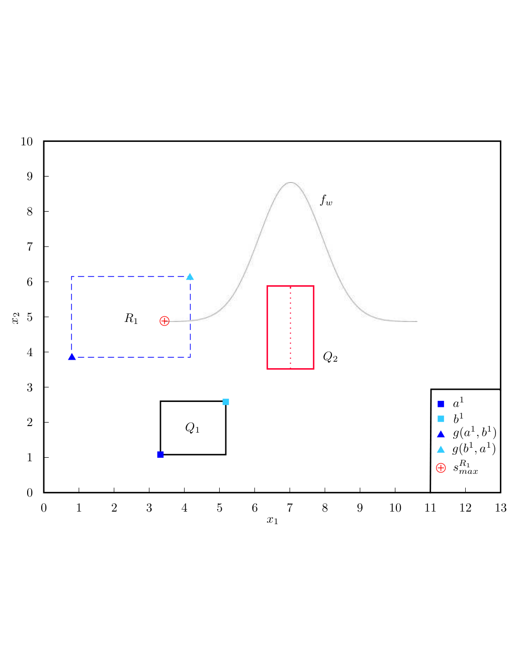
Refer to caption
Fig. 2: Depiction of the procedure for computing an upper bound on the probability of transition from Q1Q_{1} to Q2Q_{2}. First, the one-step reachable set R1R_{1} from Q1Q_{1} is over-approximated by evaluating the decomposition function at only two extremal points. Then, the distribution of z+wz+w is positioned as close to the center of Q2Q_{2} as possible under the restriction that z∈R1z\in R_{1}. A lower bound on the transition probability is achieved by positioning the distribution as far from the center of Q2Q_{2} as possible.
Lemma 1

Let ω∈Ω⊂ℝ\omega\in\Omega\subset\mathbb{R} with Ω\Omega an interval be a random variable with symmetric and unimodal probability density function fω:ℝ→ℝf_{\omega}:\mathbb{R}\rightarrow\mathbb{R} and mode c∈ℝc\in\mathbb{R}. For any a,b∈ℝa,b\in\mathbb{R} satisfying a≤ba\leq b and any r1,r2∈ℝr_{1},r_{2}\in\mathbb{R} satisfying r1≤r2r_{1}\leq r_{2}, let

sm​a​x=a+b2−c\displaystyle s_{max}=\frac{a+b}{2}-c (17)

and define

sm​a​xr\displaystyle s^{r}_{max} =arg​mins∈[r1,r2]​|smax−s|={smax,if​smax∈[r1,r2]r2,if​smax>r2r1,if​smax<r1,\displaystyle=\underset{s\in[r_{1},r_{2}]}{\argmin}|s_{max}-s|=\begin{cases}s_{max},&\text{if}\;\;s_{max}\in[r_{1},r_{2}]\\ r_{2},&\text{if}\;\;s_{max}>r_{2}\\ r_{1},&\text{if}\;\;s_{max}<r_{1},\end{cases} (18)
sm​i​nr\displaystyle s^{r}_{min} =arg​maxs∈[r1,r2]​|smax−s|={r1,if​smax<r1+r22r2,otherwise.\displaystyle=\underset{s\in[r_{1},r_{2}]}{\argmax}|s_{max}-s|=\begin{cases}r_{1},&\text{if}\;\;s_{max}<\frac{r_{1}+r_{2}}{2}\\ r_{2},&\text{otherwise}.\end{cases} (19)

Then

maxs∈[r1,r2]​∫abfω​(x−s)​𝑑x\displaystyle\underset{s\in[r_{1},r_{2}]}{\max}\int_{a}^{b}f_{\omega}(x-s)\;dx =∫abfω​(x−sm​a​xr)​𝑑x\displaystyle=\int_{a}^{b}f_{\omega}(x-s^{r}_{max})\;dx (20)
mins∈[r1,r2]​∫abfw​(x−s)​𝑑x\displaystyle\underset{s\in[r_{1},r_{2}]}{\min}\int_{a}^{b}f_{w}(x-s)\;dx =∫abfω​(x−sm​i​nr)​𝑑x.\displaystyle=\int_{a}^{b}f_{\omega}(x-s^{r}_{min})\;dx. (21)

When sm​a​x∈[r1,r2]s_{max}\in[r_{1},r_{2}] in Lemma 1, the lemma confirms the intuitive idea that the integral of a unimodal, symmetric distribution over some interval I=[a,b]I=[a,b] is maximized when the peak of its probability distribution lies at the center of II. However, for the type of systems considered in this work, the shift of such distributions will always be restricted to take values within a given rectangular set [r1,r2][r_{1},r_{2}] so that, when sm​a​x∉[r1,r2]s_{max}\not\in[r_{1},r_{2}], the shift s∈[r1,r2]s\in[r_{1},r_{2}] maximizing the overlap of the density function over II is the one closest to the global maximizing shift sm​a​xs_{max}. Conversely, a shift s∈[r1,r2]s\in[r_{1},r_{2}] minimizing this overlap is the one furthest from sm​a​xs_{max}.

Theorem 1 combines Lemma 1 and Proposition 2 to provide a procedure for constructing an IMC abstraction for (13) given a rectangular partition of its domain DD.

Theorem 1

Consider system (13) under Assumptions 1–3 and let P={Qj}j=1mP=\{Q_{j}\}_{j=1}^{m} be a rectangular partition of DD with each Qj={x:aj≤x≤bj}Q_{j}=\{x:a^{j}\leq x\leq b^{j}\} for some aj,bj∈ℝna^{j},b^{j}\in\mathbb{R}^{n} satisfying aj≤bja^{j}\leq b^{j}. For all Qj,Qℓ∈PQ_{j},Q_{\ell}\in P, let

si,m​a​xℓ\displaystyle s^{\ell}_{i,max} =aiℓ+biℓ2−ci​ for i=1,…,n,\displaystyle=\frac{a^{\ell}_{i}+b^{\ell}_{i}}{2}-c_{i}\text{ for $i=1,\ldots,n$}, (22)
 ^rj\displaystyle{\mathchoice{{\vtop{\halign{#\cr\hbox{\raise 6.25pt\hbox{\scalebox{1}[-1]{\lower 6.25pt\hbox{$\displaystyle\widehat{\vrule width=0.0pt,height=4.30554pt\vrule height=0.0pt,width=4.78937pt}$}}}}\cr\hbox{$\displaystyle r$}\crcr}}}}{{\vtop{\halign{#\cr\hbox{\raise 6.25pt\hbox{\scalebox{1}[-1]{\lower 6.25pt\hbox{$\textstyle\widehat{\vrule width=0.0pt,height=4.30554pt\vrule height=0.0pt,width=4.78937pt}$}}}}\cr\hbox{$\textstyle r$}\crcr}}}}{{\vtop{\halign{#\cr\hbox{\raise 5.81944pt\hbox{\scalebox{1}[-1]{\lower 5.81944pt\hbox{$\scriptstyle\widehat{\vrule width=0.0pt,height=3.01389pt\vrule height=0.0pt,width=3.92825pt}$}}}}\cr\hbox{$\scriptstyle r$}\crcr}}}}{{\vtop{\halign{#\cr\hbox{\raise 5.53241pt\hbox{\scalebox{1}[-1]{\lower 5.53241pt\hbox{$\scriptscriptstyle\widehat{\vrule width=0.0pt,height=2.15277pt\vrule height=0.0pt,width=3.53014pt}$}}}}\cr\hbox{$\scriptscriptstyle r$}\crcr}}}}}^{j} =g⁡(aj,bj),\displaystyle=g(a^{j},b^{j}),
r^j\displaystyle\widehat{r}^{j} =g⁡(bj,aj),\displaystyle=g(b^{j},a^{j}), (31)

and define

T^Qj→Qℓ\displaystyle\widehat{T}_{Q_{j}\rightarrow Q_{\ell}} =∏i=1n∫aiℓbiℓfwi​(xi−si,m​a​xj→ℓ)​d​xi,\displaystyle=\prod_{i=1}^{n}\int_{a^{\ell}_{i}}^{b^{\ell}_{i}}f_{w_{i}}(x_{i}-s_{i,max}^{j\rightarrow\ell})\;dx_{i}, (32)
=∏i=1n(Fwi​(biℓ−si,m​a​xj→ℓ)−Fwi​(aiℓ−si,m​a​xj→ℓ)),\displaystyle=\prod_{i=1}^{n}\bigg(F_{w_{i}}(b^{\ell}_{i}-s_{i,max}^{j\rightarrow\ell})-F_{w_{i}}(a^{\ell}_{i}-s_{i,max}^{j\rightarrow\ell})\bigg), (33)
 ^TQj→Qℓ\displaystyle{\mathchoice{{\vtop{\halign{#\cr\hbox{\raise 7.09259pt\hbox{\scalebox{1}[-1]{\lower 7.09259pt\hbox{$\displaystyle\widehat{\vrule width=0.0pt,height=6.83331pt\vrule height=0.0pt,width=7.23265pt}$}}}}\cr\hbox{$\displaystyle T$}\crcr}}}}{{\vtop{\halign{#\cr\hbox{\raise 7.09259pt\hbox{\scalebox{1}[-1]{\lower 7.09259pt\hbox{$\textstyle\widehat{\vrule width=0.0pt,height=6.83331pt\vrule height=0.0pt,width=7.23265pt}$}}}}\cr\hbox{$\textstyle T$}\crcr}}}}{{\vtop{\halign{#\cr\hbox{\raise 6.40926pt\hbox{\scalebox{1}[-1]{\lower 6.40926pt\hbox{$\scriptstyle\widehat{\vrule width=0.0pt,height=4.78334pt\vrule height=0.0pt,width=5.79965pt}$}}}}\cr\hbox{$\scriptstyle T$}\crcr}}}}{{\vtop{\halign{#\cr\hbox{\raise 5.9537pt\hbox{\scalebox{1}[-1]{\lower 5.9537pt\hbox{$\scriptscriptstyle\widehat{\vrule width=0.0pt,height=3.41667pt\vrule height=0.0pt,width=5.02959pt}$}}}}\cr\hbox{$\scriptscriptstyle T$}\crcr}}}}}_{Q_{j}\rightarrow Q_{\ell}} =∏i=1n∫aiℓbiℓfwi​(xi−si,m​i​nj→ℓ)​d​xi\displaystyle=\prod_{i=1}^{n}\int_{a^{\ell}_{i}}^{b^{\ell}_{i}}f_{w_{i}}(x_{i}-s_{i,min}^{j\rightarrow\ell})\;dx_{i}
=∏i=1n(Fwi​(biℓ−si,m​i​nj→ℓ)−Fwi​(aiℓ−si,m​i​nj→ℓ))\displaystyle=\prod_{i=1}^{n}\bigg(F_{w_{i}}(b^{\ell}_{i}-s_{i,min}^{j\rightarrow\ell})-F_{w_{i}}(a^{\ell}_{i}-s_{i,min}^{j\rightarrow\ell})\bigg) (42)

where FwiF_{w_{i}} is the cumulative distribution function for wiw_{i} and

si,m​a​xj→ℓ\displaystyle s_{i,max}^{j\rightarrow\ell} ={si,m​a​xℓ,if​si,m​a​xℓ∈[ ^rij,r^ij]r^ij,if​si,m​a​xℓ>r^ij ^rij,if​si,m​a​xℓ< ^rij,\displaystyle=\begin{cases}s^{\ell}_{i,max},&\text{if}\;\;s^{\ell}_{i,max}\in[{\mathchoice{{\vtop{\halign{#\cr\hbox{\raise 6.25pt\hbox{\scalebox{1}[-1]{\lower 6.25pt\hbox{$\displaystyle\widehat{\vrule width=0.0pt,height=4.30554pt\vrule height=0.0pt,width=4.78937pt}$}}}}\cr\hbox{$\displaystyle r$}\crcr}}}}{{\vtop{\halign{#\cr\hbox{\raise 6.25pt\hbox{\scalebox{1}[-1]{\lower 6.25pt\hbox{$\textstyle\widehat{\vrule width=0.0pt,height=4.30554pt\vrule height=0.0pt,width=4.78937pt}$}}}}\cr\hbox{$\textstyle r$}\crcr}}}}{{\vtop{\halign{#\cr\hbox{\raise 5.81944pt\hbox{\scalebox{1}[-1]{\lower 5.81944pt\hbox{$\scriptstyle\widehat{\vrule width=0.0pt,height=3.01389pt\vrule height=0.0pt,width=3.92825pt}$}}}}\cr\hbox{$\scriptstyle r$}\crcr}}}}{{\vtop{\halign{#\cr\hbox{\raise 5.53241pt\hbox{\scalebox{1}[-1]{\lower 5.53241pt\hbox{$\scriptscriptstyle\widehat{\vrule width=0.0pt,height=2.15277pt\vrule height=0.0pt,width=3.53014pt}$}}}}\cr\hbox{$\scriptscriptstyle r$}\crcr}}}}}_{i}^{j},\widehat{r}_{i}^{j}]\\ \widehat{r}^{j}_{i},&\text{if}\;\;s^{\ell}_{i,max}>\widehat{r}^{j}_{i}\\ {\mathchoice{{\vtop{\halign{#\cr\hbox{\raise 6.25pt\hbox{\scalebox{1}[-1]{\lower 6.25pt\hbox{$\displaystyle\widehat{\vrule width=0.0pt,height=4.30554pt\vrule height=0.0pt,width=4.78937pt}$}}}}\cr\hbox{$\displaystyle r$}\crcr}}}}{{\vtop{\halign{#\cr\hbox{\raise 6.25pt\hbox{\scalebox{1}[-1]{\lower 6.25pt\hbox{$\textstyle\widehat{\vrule width=0.0pt,height=4.30554pt\vrule height=0.0pt,width=4.78937pt}$}}}}\cr\hbox{$\textstyle r$}\crcr}}}}{{\vtop{\halign{#\cr\hbox{\raise 5.81944pt\hbox{\scalebox{1}[-1]{\lower 5.81944pt\hbox{$\scriptstyle\widehat{\vrule width=0.0pt,height=3.01389pt\vrule height=0.0pt,width=3.92825pt}$}}}}\cr\hbox{$\scriptstyle r$}\crcr}}}}{{\vtop{\halign{#\cr\hbox{\raise 5.53241pt\hbox{\scalebox{1}[-1]{\lower 5.53241pt\hbox{$\scriptscriptstyle\widehat{\vrule width=0.0pt,height=2.15277pt\vrule height=0.0pt,width=3.53014pt}$}}}}\cr\hbox{$\scriptscriptstyle r$}\crcr}}}}}^{j}_{i},&\text{if}\;\;s^{\ell}_{i,max}<{\mathchoice{{\vtop{\halign{#\cr\hbox{\raise 6.25pt\hbox{\scalebox{1}[-1]{\lower 6.25pt\hbox{$\displaystyle\widehat{\vrule width=0.0pt,height=4.30554pt\vrule height=0.0pt,width=4.78937pt}$}}}}\cr\hbox{$\displaystyle r$}\crcr}}}}{{\vtop{\halign{#\cr\hbox{\raise 6.25pt\hbox{\scalebox{1}[-1]{\lower 6.25pt\hbox{$\textstyle\widehat{\vrule width=0.0pt,height=4.30554pt\vrule height=0.0pt,width=4.78937pt}$}}}}\cr\hbox{$\textstyle r$}\crcr}}}}{{\vtop{\halign{#\cr\hbox{\raise 5.81944pt\hbox{\scalebox{1}[-1]{\lower 5.81944pt\hbox{$\scriptstyle\widehat{\vrule width=0.0pt,height=3.01389pt\vrule height=0.0pt,width=3.92825pt}$}}}}\cr\hbox{$\scriptstyle r$}\crcr}}}}{{\vtop{\halign{#\cr\hbox{\raise 5.53241pt\hbox{\scalebox{1}[-1]{\lower 5.53241pt\hbox{$\scriptscriptstyle\widehat{\vrule width=0.0pt,height=2.15277pt\vrule height=0.0pt,width=3.53014pt}$}}}}\cr\hbox{$\scriptscriptstyle r$}\crcr}}}}}^{j}_{i},\end{cases} (43)
si,m​i​nj→ℓ\displaystyle s_{i,min}^{j\rightarrow\ell} ={ ^rij,if​si,m​a​xℓ< ^rij+r^ij2r^ij,otherwise.\displaystyle=\begin{cases}{\mathchoice{{\vtop{\halign{#\cr\hbox{\raise 6.25pt\hbox{\scalebox{1}[-1]{\lower 6.25pt\hbox{$\displaystyle\widehat{\vrule width=0.0pt,height=4.30554pt\vrule height=0.0pt,width=4.78937pt}$}}}}\cr\hbox{$\displaystyle r$}\crcr}}}}{{\vtop{\halign{#\cr\hbox{\raise 6.25pt\hbox{\scalebox{1}[-1]{\lower 6.25pt\hbox{$\textstyle\widehat{\vrule width=0.0pt,height=4.30554pt\vrule height=0.0pt,width=4.78937pt}$}}}}\cr\hbox{$\textstyle r$}\crcr}}}}{{\vtop{\halign{#\cr\hbox{\raise 5.81944pt\hbox{\scalebox{1}[-1]{\lower 5.81944pt\hbox{$\scriptstyle\widehat{\vrule width=0.0pt,height=3.01389pt\vrule height=0.0pt,width=3.92825pt}$}}}}\cr\hbox{$\scriptstyle r$}\crcr}}}}{{\vtop{\halign{#\cr\hbox{\raise 5.53241pt\hbox{\scalebox{1}[-1]{\lower 5.53241pt\hbox{$\scriptscriptstyle\widehat{\vrule width=0.0pt,height=2.15277pt\vrule height=0.0pt,width=3.53014pt}$}}}}\cr\hbox{$\scriptscriptstyle r$}\crcr}}}}}^{j}_{i},&\text{if}\;\;s^{\ell}_{i,max}<\frac{{\mathchoice{{\vtop{\halign{#\cr\hbox{\raise 5.81944pt\hbox{\scalebox{1}[-1]{\lower 5.81944pt\hbox{$\displaystyle\widehat{\vrule width=0.0pt,height=3.01389pt\vrule height=0.0pt,width=3.92825pt}$}}}}\cr\hbox{$\displaystyle r$}\crcr}}}}{{\vtop{\halign{#\cr\hbox{\raise 5.81944pt\hbox{\scalebox{1}[-1]{\lower 5.81944pt\hbox{$\textstyle\widehat{\vrule width=0.0pt,height=3.01389pt\vrule height=0.0pt,width=3.92825pt}$}}}}\cr\hbox{$\textstyle r$}\crcr}}}}{{\vtop{\halign{#\cr\hbox{\raise 5.51805pt\hbox{\scalebox{1}[-1]{\lower 5.51805pt\hbox{$\scriptstyle\widehat{\vrule width=0.0pt,height=2.10971pt\vrule height=0.0pt,width=2.34679pt}$}}}}\cr\hbox{$\scriptstyle r$}\crcr}}}}{{\vtop{\halign{#\cr\hbox{\raise 5.31712pt\hbox{\scalebox{1}[-1]{\lower 5.31712pt\hbox{$\scriptscriptstyle\widehat{\vrule width=0.0pt,height=1.50694pt\vrule height=0.0pt,width=1.67627pt}$}}}}\cr\hbox{$\scriptscriptstyle r$}\crcr}}}}}^{j}_{i}+\widehat{r}^{j}_{i}}{2}\\ \widehat{r}^{j}_{i},&\text{otherwise}.\end{cases} (44)

Then ℐ=(P,
 

 ^

 
T
,T^)
\mathcal{I}=(P,{\mathchoice{{\vtop{\halign{#\cr\hbox{\raise 7.09259pt\hbox{\scalebox{1}[-1]{\lower 7.09259pt\hbox{$\displaystyle\widehat{\vrule width=0.0pt,height=6.83331pt\vrule height=0.0pt,width=7.23265pt}$}}}}\cr\hbox{$\displaystyle T$}\crcr}}}}{{\vtop{\halign{#\cr\hbox{\raise 7.09259pt\hbox{\scalebox{1}[-1]{\lower 7.09259pt\hbox{$\textstyle\widehat{\vrule width=0.0pt,height=6.83331pt\vrule height=0.0pt,width=7.23265pt}$}}}}\cr\hbox{$\textstyle T$}\crcr}}}}{{\vtop{\halign{#\cr\hbox{\raise 6.40926pt\hbox{\scalebox{1}[-1]{\lower 6.40926pt\hbox{$\scriptstyle\widehat{\vrule width=0.0pt,height=4.78334pt\vrule height=0.0pt,width=5.79965pt}$}}}}\cr\hbox{$\scriptstyle T$}\crcr}}}}{{\vtop{\halign{#\cr\hbox{\raise 5.9537pt\hbox{\scalebox{1}[-1]{\lower 5.9537pt\hbox{$\scriptscriptstyle\widehat{\vrule width=0.0pt,height=3.41667pt\vrule height=0.0pt,width=5.02959pt}$}}}}\cr\hbox{$\scriptscriptstyle T$}\crcr}}}}},\widehat{T})
is an IMC abstraction of (13).

Theorem 1 provides the mathematical foundation for solving Subproblem 1. Given a system of the form (13) satisfying Assumptions 1 to 3, and a rectangular partition PP, this theorem shows that an IMC abstraction of (13) can be computed efficiently. Specifically, for any state in PP, we establish an over-approximation of its one-step reachable set by evaluating the system’s decomposition function at only two points. Finding the maximizing and minimizing shifts inside the reachable sets decouples along each coordinate and involves a number of operations that is linear in the dimension nn of the state-space, according to (43) and (44). Finally, we see in (32) and (1) that nn integral evaluations are needed per transition bound. This last step requires two evaluations of FwiF_{w_{i}} per bound for each ii and thus amounts to 2​n2n function evaluations per bound. Because the computed over-approximations of reachable sets for mixed monotone dynamics were shown to be tight in certain cases [16], our abstraction technique is generally not as conservative as those employing Lipschitz constants [29], while being computationally efficient.

V Verification of IMCs

In this section, we develop the machinery to address Subproblem 2. Let ℐ\mathcal{I} be an IMC abstraction of (1) obtained from, e.g., the abstraction approach in Section IV for systems with specific form (13). For a formula ϕ\phi of the type (2), our goal is to sort the initial states of ℐ\mathcal{I} into the sets Qϕy​e​s,Qϕn​oQ^{yes}_{\phi},Q^{no}_{\phi} and Qϕ?Q^{?}_{\phi}. To this end, for any initial state QjQ_{j} of ℐ\mathcal{I}, we require a lower bound and an upper bound on the probability of satisfying the ω\omega-regular property Ψ\Psi for the probabilistic specification ϕ=𝒫⋈ps​a​t​[Ψ]\phi=\mathcal{P}_{\bowtie p_{sat}}[\Psi]. We thus seek to compute the greatest lower bound
 

 ^

 
𝒫
ℐ
​(Qj⊧Ψ)
{\mathchoice{{\vtop{\halign{#\cr\hbox{\raise 7.09259pt\hbox{\scalebox{1}[-1]{\lower 7.09259pt\hbox{$\displaystyle\widehat{\vrule width=0.0pt,height=6.83331pt\vrule height=0.0pt,width=6.80557pt}$}}}}\cr\hbox{$\displaystyle\mathcal{P}$}\crcr}}}}{{\vtop{\halign{#\cr\hbox{\raise 7.09259pt\hbox{\scalebox{1}[-1]{\lower 7.09259pt\hbox{$\textstyle\widehat{\vrule width=0.0pt,height=6.83331pt\vrule height=0.0pt,width=6.80557pt}$}}}}\cr\hbox{$\textstyle\mathcal{P}$}\crcr}}}}{{\vtop{\halign{#\cr\hbox{\raise 6.40926pt\hbox{\scalebox{1}[-1]{\lower 6.40926pt\hbox{$\scriptstyle\widehat{\vrule width=0.0pt,height=4.78334pt\vrule height=0.0pt,width=5.37502pt}$}}}}\cr\hbox{$\scriptstyle\mathcal{P}$}\crcr}}}}{{\vtop{\halign{#\cr\hbox{\raise 5.94775pt\hbox{\scalebox{1}[-1]{\lower 5.94775pt\hbox{$\scriptscriptstyle\widehat{\vrule width=0.0pt,height=3.3988pt\vrule height=0.0pt,width=4.50006pt}$}}}}\cr\hbox{$\scriptscriptstyle\mathcal{P}$}\crcr}}}}}_{\mathcal{I}}(Q_{j}\models\Psi)
and least upper bound 𝒫^ℐ​(Qj⊧Ψ)\widehat{\mathcal{P}}_{\mathcal{I}}(Q_{j}\models\Psi) such that, for any adversary ν∈νℐ\nu\in\nu_{\mathcal{I}},

 ^𝒫ℐ​(Qj⊧Ψ)≤𝒫ℐ⁡[ν]​(Qj⊧Ψ)≤𝒫^ℐ​(Qj⊧Ψ).\displaystyle{\mathchoice{{\vtop{\halign{#\cr\hbox{\raise 7.09259pt\hbox{\scalebox{1}[-1]{\lower 7.09259pt\hbox{$\displaystyle\widehat{\vrule width=0.0pt,height=6.83331pt\vrule height=0.0pt,width=6.80557pt}$}}}}\cr\hbox{$\displaystyle\mathcal{P}$}\crcr}}}}{{\vtop{\halign{#\cr\hbox{\raise 7.09259pt\hbox{\scalebox{1}[-1]{\lower 7.09259pt\hbox{$\textstyle\widehat{\vrule width=0.0pt,height=6.83331pt\vrule height=0.0pt,width=6.80557pt}$}}}}\cr\hbox{$\textstyle\mathcal{P}$}\crcr}}}}{{\vtop{\halign{#\cr\hbox{\raise 6.40926pt\hbox{\scalebox{1}[-1]{\lower 6.40926pt\hbox{$\scriptstyle\widehat{\vrule width=0.0pt,height=4.78334pt\vrule height=0.0pt,width=5.37502pt}$}}}}\cr\hbox{$\scriptstyle\mathcal{P}$}\crcr}}}}{{\vtop{\halign{#\cr\hbox{\raise 5.94775pt\hbox{\scalebox{1}[-1]{\lower 5.94775pt\hbox{$\scriptscriptstyle\widehat{\vrule width=0.0pt,height=3.3988pt\vrule height=0.0pt,width=4.50006pt}$}}}}\cr\hbox{$\scriptscriptstyle\mathcal{P}$}\crcr}}}}}_{\mathcal{I}}(Q_{j}\models\Psi)\leq\mathcal{P}_{\mathcal{I}[\nu]}(Q_{j}\models\Psi)\leq\widehat{\mathcal{P}}_{\mathcal{I}}(Q_{j}\models\Psi)\;.

Our approach draws from the verification of regular MCs against ω\omega-regular properties using automata-based methods [1, Section 10.3]. First, we generate a DRA 𝒜\mathcal{A} that recognizes the language induced by property Ψ\Psi. Such a DRA always exists. Several algorithms can generate a DRA for a large subset of ω\omega-regular expressions [30] [31]. Then, we construct the product ℐ⊗𝒜\mathcal{I}\otimes\mathcal{A} as defined below.

Definition 7 (Product Interval-valued Markov Chain)

Let ℐ=(Q,
 

 ^

 
T
,T^,Σ,L)
\mathcal{I}=(Q,{\mathchoice{{\vtop{\halign{#\cr\hbox{\raise 7.09259pt\hbox{\scalebox{1}[-1]{\lower 7.09259pt\hbox{$\displaystyle\widehat{\vrule width=0.0pt,height=6.83331pt\vrule height=0.0pt,width=7.23265pt}$}}}}\cr\hbox{$\displaystyle T$}\crcr}}}}{{\vtop{\halign{#\cr\hbox{\raise 7.09259pt\hbox{\scalebox{1}[-1]{\lower 7.09259pt\hbox{$\textstyle\widehat{\vrule width=0.0pt,height=6.83331pt\vrule height=0.0pt,width=7.23265pt}$}}}}\cr\hbox{$\textstyle T$}\crcr}}}}{{\vtop{\halign{#\cr\hbox{\raise 6.40926pt\hbox{\scalebox{1}[-1]{\lower 6.40926pt\hbox{$\scriptstyle\widehat{\vrule width=0.0pt,height=4.78334pt\vrule height=0.0pt,width=5.79965pt}$}}}}\cr\hbox{$\scriptstyle T$}\crcr}}}}{{\vtop{\halign{#\cr\hbox{\raise 5.9537pt\hbox{\scalebox{1}[-1]{\lower 5.9537pt\hbox{$\scriptscriptstyle\widehat{\vrule width=0.0pt,height=3.41667pt\vrule height=0.0pt,width=5.02959pt}$}}}}\cr\hbox{$\scriptscriptstyle T$}\crcr}}}}},\widehat{T},\Sigma,L)
be an Interval-valued Markov Chain and 𝒜=(S,Σ,δ,s0,A​c​c)\mathcal{A}=(S,\Sigma,\delta,s_{0},Acc) be a Deterministic Rabin Automaton. The product ℐ⊗𝒜=(Q×S,
 

 ^

 
T′
,T′^,A​c​c′,L′)
\mathcal{I}\otimes\mathcal{A}=(Q\times S,{\mathchoice{{\vtop{\halign{#\cr\hbox{\raise 7.48743pt\hbox{\scalebox{1}[-1]{\lower 7.48743pt\hbox{$\displaystyle\widehat{\vrule width=0.0pt,height=8.01782pt\vrule height=0.0pt,width=10.03821pt}$}}}}\cr\hbox{$\displaystyle T^{\prime}$}\crcr}}}}{{\vtop{\halign{#\cr\hbox{\raise 7.32076pt\hbox{\scalebox{1}[-1]{\lower 7.32076pt\hbox{$\textstyle\widehat{\vrule width=0.0pt,height=7.51782pt\vrule height=0.0pt,width=10.03821pt}$}}}}\cr\hbox{$\textstyle T^{\prime}$}\crcr}}}}{{\vtop{\halign{#\cr\hbox{\raise 6.74667pt\hbox{\scalebox{1}[-1]{\lower 6.74667pt\hbox{$\scriptstyle\widehat{\vrule width=0.0pt,height=5.7956pt\vrule height=0.0pt,width=8.50453pt}$}}}}\cr\hbox{$\scriptstyle T^{\prime}$}\crcr}}}}{{\vtop{\halign{#\cr\hbox{\raise 6.22223pt\hbox{\scalebox{1}[-1]{\lower 6.22223pt\hbox{$\scriptscriptstyle\widehat{\vrule width=0.0pt,height=4.22223pt\vrule height=0.0pt,width=7.73447pt}$}}}}\cr\hbox{$\scriptscriptstyle T^{\prime}$}\crcr}}}}},\widehat{T^{\prime}},Acc^{\prime},L^{\prime})
is an Interval-valued Markov Chain where:

  • •

    Q×SQ\times S is a set of states,

  • •

    {(Qj,s0):Qj∈Q}\{(Q_{j},s_{0}):Q_{j}\in Q\} is a finite set of initial states,

  • •


     ^

     
    T′
    ⟨Qj,s⟩→⟨Qℓ,s′⟩
    ={
     

     ^

     
    T′
    Qj→Qℓ
    ,if​s′=δ⁡(s,L⁡(Qℓ))
             0,otherwise
    {\mathchoice{{\vtop{\halign{#\cr\hbox{\raise 7.48743pt\hbox{\scalebox{1}[-1]{\lower 7.48743pt\hbox{$\displaystyle\widehat{\vrule width=0.0pt,height=8.01782pt\vrule height=0.0pt,width=10.03821pt}$}}}}\cr\hbox{$\displaystyle T^{\prime}$}\crcr}}}}{{\vtop{\halign{#\cr\hbox{\raise 7.32076pt\hbox{\scalebox{1}[-1]{\lower 7.32076pt\hbox{$\textstyle\widehat{\vrule width=0.0pt,height=7.51782pt\vrule height=0.0pt,width=10.03821pt}$}}}}\cr\hbox{$\textstyle T^{\prime}$}\crcr}}}}{{\vtop{\halign{#\cr\hbox{\raise 6.74667pt\hbox{\scalebox{1}[-1]{\lower 6.74667pt\hbox{$\scriptstyle\widehat{\vrule width=0.0pt,height=5.7956pt\vrule height=0.0pt,width=8.50453pt}$}}}}\cr\hbox{$\scriptstyle T^{\prime}$}\crcr}}}}{{\vtop{\halign{#\cr\hbox{\raise 6.22223pt\hbox{\scalebox{1}[-1]{\lower 6.22223pt\hbox{$\scriptscriptstyle\widehat{\vrule width=0.0pt,height=4.22223pt\vrule height=0.0pt,width=7.73447pt}$}}}}\cr\hbox{$\scriptscriptstyle T^{\prime}$}\crcr}}}}}_{\left<Q_{j},s\right>\rightarrow\left<Q_{\ell},s^{\prime}\right>}=\begin{cases}{\mathchoice{{\vtop{\halign{#\cr\hbox{\raise 7.48743pt\hbox{\scalebox{1}[-1]{\lower 7.48743pt\hbox{$\displaystyle\widehat{\vrule width=0.0pt,height=8.01782pt\vrule height=0.0pt,width=10.03821pt}$}}}}\cr\hbox{$\displaystyle T^{\prime}$}\crcr}}}}{{\vtop{\halign{#\cr\hbox{\raise 7.32076pt\hbox{\scalebox{1}[-1]{\lower 7.32076pt\hbox{$\textstyle\widehat{\vrule width=0.0pt,height=7.51782pt\vrule height=0.0pt,width=10.03821pt}$}}}}\cr\hbox{$\textstyle T^{\prime}$}\crcr}}}}{{\vtop{\halign{#\cr\hbox{\raise 6.74667pt\hbox{\scalebox{1}[-1]{\lower 6.74667pt\hbox{$\scriptstyle\widehat{\vrule width=0.0pt,height=5.7956pt\vrule height=0.0pt,width=8.50453pt}$}}}}\cr\hbox{$\scriptstyle T^{\prime}$}\crcr}}}}{{\vtop{\halign{#\cr\hbox{\raise 6.22223pt\hbox{\scalebox{1}[-1]{\lower 6.22223pt\hbox{$\scriptscriptstyle\widehat{\vrule width=0.0pt,height=4.22223pt\vrule height=0.0pt,width=7.73447pt}$}}}}\cr\hbox{$\scriptscriptstyle T^{\prime}$}\crcr}}}}}_{Q_{j}\rightarrow Q_{\ell}},\;\;\text{if}\;\;s^{\prime}=\delta(s,L(Q_{\ell}))\\ \;\;\;\;\;\;\;\;\;0,\;\;\;\;\;\;\text{otherwise}\end{cases}


  • •

    T′^⟨Qj,s⟩→⟨Qℓ,s′⟩={T′^Qj→Qℓ,if​s′=δ⁡(s,L⁡(Qℓ))         0,otherwise\widehat{T^{\prime}}_{\left<Q_{j},s\right>\rightarrow\left<Q_{\ell},s^{\prime}\right>}=\begin{cases}\widehat{T^{\prime}}_{Q_{j}\rightarrow Q_{\ell}},\;\;\text{if}\;\;s^{\prime}=\delta(s,L(Q_{\ell}))\\ \;\;\;\;\;\;\;\;\;0,\;\;\;\;\;\;\text{otherwise}\end{cases}

  • •

    A​c​c′={E1,E2,…,Ek,F1,F2,…,Fk}Acc^{\prime}=\{E_{1},E_{2},\ldots,E_{k},F_{1},F_{2},\ldots,F_{k}\} is a set of atomic propositions, where EiE_{i} and FiF_{i} are the sets in the Rabin pairs of A​c​cAcc,

  • •

    L′:Q×S→2A​c​c′L^{\prime}:Q\times S\rightarrow 2^{Acc^{\prime}} such that H∈L′​(⟨Qj,s⟩)H\in L^{\prime}(\left<Q_{j},s\right>) if and only if s∈Hs\in H, for all H∈A​c​c′H\in Acc^{\prime} and for all jj.

A MC induced by ℐ⊗𝒜\mathcal{I}\otimes\mathcal{A} is called a product Markov Chain, and we use the notation ℳ⊗𝒜\mathcal{M}_{\otimes}^{\mathcal{A}} to denote such an induced MC.

The probability of satisfying Ψ\Psi from initial state QjQ_{j} in a discrete-time MC equals that of reaching an accepting Bottom Strongly Connected Component (BSCC) from initial state ⟨Qj,s0⟩\left<Q_{j},s_{0}\right> in the product MC with 𝒜\mathcal{A} [1].

Definition 8 (Bottom Strongly Connected Component)

Given a Markov Chain ℳ\mathcal{M} with states QQ, a set B⊆QB\subseteq Q is a Bottom Strongly Connected Component (BSCC) of ℳ\mathcal{M} if

  • •

    BB is strongly connected: for each pair of states (q,t)(q,t) in BB, there exists a path q0​q1​…​qnq_{0}q_{1}\ldots q_{n} such that T⁡(qi,qi+1)>0T(q_{i},q_{i+1})>0, i=0,1,…,n−1i=0,1,\ldots,n-1, and qi∈Bq_{i}\in B for 0≤i≤n0\leq i\leq n with q0=q,q_{0}=q, qn=tq_{n}=t,

  • •

    no proper superset of BB is strongly connected,

  • •

    ∀s∈B\forall s\in B, Σt∈B​T​(s,t)=1\Sigma_{t\in B}T(s,t)=1.

In words, every state in a BSCC BB is reachable from any state in BB, and every state in BB only transitions to another state in BB. Moreover, BB is accepting when at least one of its states maps to the accepting set of a Rabin pair, while no state in BB maps to the non-accepting set of that same pair.

Definition 9 (Accepting Bottom Strongly Connected Component)

A Bottom Strongly Connected Component BB of a product MC ℳ⊗𝒜\mathcal{M}_{\otimes}^{\mathcal{A}} is said to be accepting if:

∃i:\displaystyle\exists i: (∃⟨Qj,sℓ⟩∈B.Fi∈L′(⟨Qj,sℓ⟩))\displaystyle\Big(\;\exists\left<Q_{j},s_{\ell}\right>\in B\;.\;F_{i}\in L^{\prime}(\left<Q_{j},s_{\ell}\right>)\;\Big)
∧(∀⟨Qj,sℓ⟩∈B.Ei∉L′(⟨Qj,sℓ⟩)).\displaystyle\wedge\Big(\;\forall\left<Q_{j},s_{\ell}\right>\in B\;.\;E_{i}\not\in L^{\prime}(\left<Q_{j},s_{\ell}\right>)\;\Big). (53)

Definition 10 (Non-Accepting Bottom Strongly Connected Component)

A Bottom Strongly Connected Component BB of a product MC ℳ⊗𝒜\mathcal{M}_{\otimes}^{\mathcal{A}} is said to be non-accepting if it is not accepting.

We denote by UAU^{A} and UNU^{N} the sets of states that respectively belong to an accepting and a non-accepting BSCC in a product MC.

Note that each product MC ℳ⊗𝒜\mathcal{M}_{\otimes}^{\mathcal{A}} induced by ℐ⊗𝒜\mathcal{I}\otimes\mathcal{A} simulates the behavior of ℐ\mathcal{I} under some adversary ν∈νℐ\mathcal{\nu}\in\mathcal{\nu}_{\mathcal{I}}. Indeed, for any two states QjQ_{j} and QℓQ_{\ell} in ℐ\mathcal{I} and some states s,s′,s′′s,s^{\prime},s^{\prime\prime} and s′′′s^{\prime\prime\prime} in 𝒜\mathcal{A}, we allow T⟨Qj,s⟩→⟨Qℓ,s′⟩T_{\left<Q_{j},s\right>\rightarrow\left<Q_{\ell},s^{\prime}\right>} and T⟨Qj,s′′⟩→⟨Qℓ,s′′′⟩T_{\left<Q_{j},s^{\prime\prime}\right>\rightarrow\left<Q_{\ell},s^{\prime\prime\prime}\right>} to assume different values in ℳ⊗𝒜\mathcal{M}_{\otimes}^{\mathcal{A}}, which means that the transition probability between QjQ_{j} and QℓQ_{\ell} may change depending on the history of the path in ℐ\mathcal{I} as encoded in the state of 𝒜\mathcal{A}.

Also, the adversary is history-independent or memoryless in the product automaton, that is, the adversary’s chosen transition probability only depends on the current states of the IMC and the DRA 𝒜\mathcal{A}. For reachability problems in IMCs, it was shown in [32] that memoryless adversaries yield the same bounds as the memory-dependent ones. The following facts establish that, therefore, such memoryless (in the product) adversaries are sufficient for IMC verification.

Fact 2

[1, p. 792, Theorem 10.56] [32] We denote the set of adversaries of ℐ\mathcal{I} that are memoryless in the product IMC ℐ⊗𝒜\mathcal{I}\otimes\mathcal{A} by (νℐ)⊗𝒜⊆νℐ(\mathcal{\nu}_{\mathcal{I}})_{\otimes}^{\mathcal{A}}\subseteq\mathcal{\nu}_{\mathcal{I}}. It holds that

infν∈νℐ𝒫ℐ⁡[ν]​(Qi⊧Ψ)\displaystyle\inf_{\nu\in\nu_{\mathcal{I}}}\mathcal{P}_{\mathcal{I}[\mathcal{\nu}]}(Q_{i}\models\Psi) =infν∈(νℐ)⊗𝒜𝒫ℐ⁡[ν]​(Qi⊧Ψ)\displaystyle=\inf_{\nu\in(\mathcal{\nu}_{\mathcal{I}})_{\otimes}^{\mathcal{A}}}\mathcal{P}_{\mathcal{I}[\mathcal{\nu}]}(Q_{i}\models\Psi) (54)
supν∈νℐ𝒫ℐ⁡[ν]​(Qi⊧Ψ)\displaystyle\sup_{\nu\in\nu_{\mathcal{I}}}\mathcal{P}_{\mathcal{I}[\mathcal{\nu}]}(Q_{i}\models\Psi) =supν∈(νℐ)⊗𝒜𝒫ℐ⁡[ν]​(Qi⊧Ψ).\displaystyle=\sup_{\nu\in(\mathcal{\nu}_{\mathcal{I}})_{\otimes}^{\mathcal{A}}}\mathcal{P}_{\mathcal{I}[\mathcal{\nu}]}(Q_{i}\models\Psi)\ . (55)

Fact 3

For any adversary ν∈(νℐ)⊗𝒜\mathcal{\nu}\in(\mathcal{\nu}_{\mathcal{I}})_{\otimes}^{\mathcal{A}} in ℐ\mathcal{I}, it holds that 𝒫ℐ⁡[ν]​(Qi⊧Ψ)\mathcal{P}_{\mathcal{I}[\nu]}(Q_{i}\models\Psi) = 𝒫(ℳ⊗𝒜)ν​(⟨Qi,s0⟩⊧◇​UA)\mathcal{P}_{(\mathcal{M}_{\otimes}^{\mathcal{A}})_{\nu}}(\left<Q_{i},s_{0}\right>\models\Diamond U^{A}), where (ℳ⊗𝒜)ν(\mathcal{M}_{\otimes}^{\mathcal{A}})_{\nu} denotes the product MC induced by ℐ⊗𝒜\mathcal{I}\otimes\mathcal{A} corresponding to adversary ν\nu.

Consequently, computing
 

 ^

 
𝒫
ℐ
​(Qi⊧Ψ)
{\mathchoice{{\vtop{\halign{#\cr\hbox{\raise 7.09259pt\hbox{\scalebox{1}[-1]{\lower 7.09259pt\hbox{$\displaystyle\widehat{\vrule width=0.0pt,height=6.83331pt\vrule height=0.0pt,width=6.80557pt}$}}}}\cr\hbox{$\displaystyle\mathcal{P}$}\crcr}}}}{{\vtop{\halign{#\cr\hbox{\raise 7.09259pt\hbox{\scalebox{1}[-1]{\lower 7.09259pt\hbox{$\textstyle\widehat{\vrule width=0.0pt,height=6.83331pt\vrule height=0.0pt,width=6.80557pt}$}}}}\cr\hbox{$\textstyle\mathcal{P}$}\crcr}}}}{{\vtop{\halign{#\cr\hbox{\raise 6.40926pt\hbox{\scalebox{1}[-1]{\lower 6.40926pt\hbox{$\scriptstyle\widehat{\vrule width=0.0pt,height=4.78334pt\vrule height=0.0pt,width=5.37502pt}$}}}}\cr\hbox{$\scriptstyle\mathcal{P}$}\crcr}}}}{{\vtop{\halign{#\cr\hbox{\raise 5.94775pt\hbox{\scalebox{1}[-1]{\lower 5.94775pt\hbox{$\scriptscriptstyle\widehat{\vrule width=0.0pt,height=3.3988pt\vrule height=0.0pt,width=4.50006pt}$}}}}\cr\hbox{$\scriptscriptstyle\mathcal{P}$}\crcr}}}}}_{\mathcal{I}}(Q_{i}\models\Psi)
and 𝒫^ℐ​(Qi⊧Ψ)\widehat{\mathcal{P}}_{\mathcal{I}}(Q_{i}\models\Psi) amounts to finding the product MCs induced by ℐ⊗𝒜\mathcal{I}\otimes\mathcal{A} that respectively minimize and maximize the probability of reaching an accepting BSCC from ⟨Qj,s0⟩\left<Q_{j},s_{0}\right>. Such reachability problems in IMCs were solved when the destination states are fixed for all induced MCs [33] [12].

However, in general, the sets UAU^{A} and UNU^{N} are not fixed in product IMCs and vary with the assumed values for each transition. Specifically, UAU^{A} and UNU^{N} are determined by transitions that are either “on” or “off”, i.e. those whose lower bound is zero and upper bound is non-zero, as seen in the example in Fig. 3: in the product MC (ℳ⊗𝒜)1(\mathcal{M}_{\otimes}^{\mathcal{A}})_{1} induced by ℐ⊗𝒜\mathcal{I}\otimes\mathcal{A}, UAU^{A} is {Q0,Q1}\{Q_{0},Q_{1}\} while {Q2}\{Q_{2}\} is non-accepting. In (ℳ⊗𝒜)2(\mathcal{M}_{\otimes}^{\mathcal{A}})_{2}, another product MC induced by ℐ⊗𝒜\mathcal{I}\otimes\mathcal{A}, all states are in UNU^{N}.

Fig. 3: Two product MCs (ℳ⊗𝒜)1(\mathcal{M}_{\otimes}^{\mathcal{A}})_{1} and (ℳ⊗𝒜)2(\mathcal{M}_{\otimes}^{\mathcal{A}})_{2} induced by a product IMC ℐ⊗𝒜\mathcal{I}\otimes\mathcal{A}. Accepting BSCCs are shown in green; non-accepting BSCCs are red. In (ℳ⊗𝒜)1(\mathcal{M}_{\otimes}^{\mathcal{A}})_{1}, UA={Q0,Q1}U^{A}=\{Q_{0},Q_{1}\} and UN={Q2}U^{N}=\{Q_{2}\}; in (ℳ⊗𝒜)2(\mathcal{M}_{\otimes}^{\mathcal{A}})_{2}, UA=∅U^{A}=\emptyset and UN={Q0,Q1,Q2}U^{N}=\{Q_{0},Q_{1},Q_{2}\}.

The contribution of this paper to the verification of IMCs for ω\omega-regular properties is twofold. First, we show that a product IMC always induces a largest Losing Component and Winning Component. These components contain states that reach a BSCC with probability 1. Upper and lower bounds on Ψ\Psi are computed by solving a reachability problem for these sets. We further introduce the notion of Permanent Losing Components and Permanent Winning Components which play a crucial role in the refinement algorithm derived in Section VI. Second, we describe a graph search algorithm to find these components.

V-A Computation of Satisfiability Bounds in IMCs

Previous works highlighted the crucial role of BSCCs in product MCs [1, Theorem 10.56]. As the probability of reaching an accepting BSCC in a product MC determines the probability of satisfying some property in the original abstraction, we now further introduce the notions of winning and losing components. These components include states that may not belong to a BSCC but from which any path is bound to reach a BSCC.

Definition 11 (Winning/Losing Component)

[25] A winning (losing) component W​C​(L​C)WC\;(LC) of a product MC ℳ⊗𝒜\mathcal{M}_{\otimes}^{\mathcal{A}} is a set of states satisfying 𝒫ℳ⊗𝒜​(W​C⊧◇​UA)=1​(𝒫ℳ⊗𝒜​(L​C⊧◇​UN)=1)\mathcal{P}_{\mathcal{M}_{\otimes}^{\mathcal{A}}}(WC\models\Diamond U^{A})=1\;(\;\mathcal{P}_{\mathcal{M}_{\otimes}^{\mathcal{A}}}(LC\models\Diamond U^{N})=1\;) , where UAU^{A} (UNU^{N}) is the set of states belonging to an accepting (non-accepting) BSCC in ℳ⊗𝒜\mathcal{M}_{\otimes}^{\mathcal{A}}.

It naturally follows that the probability of eventually reaching a BSCC from some initial state is equal to that of reaching a winning or losing component.

Corollary 1

In any product MC ℳ⊗𝒜\mathcal{M}_{\otimes}^{\mathcal{A}},

𝒫ℳ⊗𝒜​(⟨Qi,s0⟩⊧◇​UA)\displaystyle\mathcal{P}_{\mathcal{M}_{\otimes}^{\mathcal{A}}}(\left<Q_{i},s_{0}\right>\models\Diamond U^{A}) =𝒫ℳ⊗𝒜​(⟨Qi,s0⟩⊧◇​W​C)\displaystyle=\mathcal{P}_{\mathcal{M}_{\otimes}^{\mathcal{A}}}(\left<Q_{i},s_{0}\right>\models\Diamond WC) (56)
𝒫ℳ⊗𝒜​(⟨Qi,s0⟩⊧◇​UN)\displaystyle\mathcal{P}_{\mathcal{M}_{\otimes}^{\mathcal{A}}}(\left<Q_{i},s_{0}\right>\models\Diamond U^{N}) =𝒫ℳ⊗𝒜​(⟨Qi,s0⟩⊧◇​L​C).\displaystyle=\mathcal{P}_{\mathcal{M}_{\otimes}^{\mathcal{A}}}(\left<Q_{i},s_{0}\right>\models\Diamond LC)\;. (57)

For any initial state in a product IMC, our goal is thus to find induced product MCs that minimize and maximize the probability of reaching a winning component.

We refer to the technical appendix for all lemmas and proofs leading to the proposed solution. The key observation is that any product IMC induces a largest winning component and a largest losing component. The largest winning component is the set of states of the product IMC belonging to a winning component for at least one induced product MC, while the largest losing component is the analogous set for losing components. Definitions of permanent and potential components follow directly from that of largest components.

Definition 12 (Largest Winning/Losing Components)

A state ⟨Qi,sj⟩∈Q×S\left<Q_{i},s_{j}\right>\in Q\times S of a product IMC ℐ⊗𝒜\mathcal{I}\otimes\mathcal{A} is a member of the Largest Winning (Losing) Component (W​C)L(WC)_{L} ((L​C)L)\big(\;(LC)_{L}\;\big) if there exists a product MC induced by ℐ⊗𝒜\mathcal{I}\otimes\mathcal{A} such that ⟨Qi,sj⟩\left<Q_{i},s_{j}\right> is a winning (losing) component.

Definition 13 (Permanent Winning/Losing Components)

A state ⟨Qi,sj⟩∈Q×S\left<Q_{i},s_{j}\right>\in Q\times S of a product IMC ℐ⊗𝒜\mathcal{I}\otimes\mathcal{A} is a member of the Permanent Winning (Losing) Component (W​C)P(WC)_{P} ((L​C)P)\big(\;(LC)_{P}\;\big) of ℐ⊗𝒜\mathcal{I}\otimes\mathcal{A} if ⟨Qi,sj⟩\left<Q_{i},s_{j}\right> is a winning (losing) component for all product MCs induced by ℐ⊗𝒜\mathcal{I}\otimes\mathcal{A}.

Definition 14 (Potential Winning/Losing Components)

A state ⟨Qi,sj⟩∈Q×S\left<Q_{i},s_{j}\right>\in Q\times S of a product IMC ℐ⊗𝒜\mathcal{I}\otimes\mathcal{A} is a member of the Potential Winning (Losing) Component (W​C)?(WC)_{?} ((L​C)?)\big(\;(LC)_{?}\;\big) of ℐ⊗𝒜\mathcal{I}\otimes\mathcal{A} if ⟨Qi,sj⟩∈(W​C)L∖(W​C)P​(⟨Qi,sj⟩∈(L​C)L∖(L​C)P)\left<Q_{i},s_{j}\right>\in(WC)_{L}\setminus(WC)_{P}\;\;\big(\left<Q_{i},s_{j}\right>\in\;(LC)_{L}\setminus(LC)_{P}\;\big).

Note that the sets (W​C)?(WC)_{?} and (L​C)?(LC)_{?} may intersect, and by extension (W​C)L(WC)_{L} and (L​C)L(LC)_{L}, while (W​C)P(WC)_{P} and (L​C)P(LC)_{P} are disjoint. An important result established in this paper is that any product IMC induces a set of product MCs where all members of the largest winning component belong to a winning component simultaneously. A product IMC induces an analogous set of product MCs for the largest losing component. We provide proofs in Lemmas 5-7 of the Appendix.

We now state the main result of this section, which establishes that bounds on the probability of satisfying an ω\omega-regular property in an IMC can be computed by solving a reachability maximization problem on a fixed set of states in a product IMC. These sets are the largest components of the product IMC. Furthermore, solving these problems induce sets of best and worst-case product MCs where the probabilities of reaching a winning component are respectively maximized and minimized for all initial states of the product IMC.

Theorem 2

Let ℐ\mathcal{I} be an IMC and 𝒜\mathcal{A} be a Rabin Automaton corresponding to omega-regular property Ψ\Psi. Let (W​C)L(WC)_{L} and (L​C)L(LC)_{L} be the largest winning and losing components and (W​C)P(WC)_{P} and (L​C)P(LC)_{P} be the permanent winning and losing components of the product IMC ℐ⊗𝒜\mathcal{I}\otimes\mathcal{A}. Then for any initial state QiQ_{i} of ℐ\mathcal{I},

 ^𝒫ℐ​(Qi⊧Ψ)\displaystyle{\mathchoice{{\vtop{\halign{#\cr\hbox{\raise 7.09259pt\hbox{\scalebox{1}[-1]{\lower 7.09259pt\hbox{$\displaystyle\widehat{\vrule width=0.0pt,height=6.83331pt\vrule height=0.0pt,width=6.80557pt}$}}}}\cr\hbox{$\displaystyle\mathcal{P}$}\crcr}}}}{{\vtop{\halign{#\cr\hbox{\raise 7.09259pt\hbox{\scalebox{1}[-1]{\lower 7.09259pt\hbox{$\textstyle\widehat{\vrule width=0.0pt,height=6.83331pt\vrule height=0.0pt,width=6.80557pt}$}}}}\cr\hbox{$\textstyle\mathcal{P}$}\crcr}}}}{{\vtop{\halign{#\cr\hbox{\raise 6.40926pt\hbox{\scalebox{1}[-1]{\lower 6.40926pt\hbox{$\scriptstyle\widehat{\vrule width=0.0pt,height=4.78334pt\vrule height=0.0pt,width=5.37502pt}$}}}}\cr\hbox{$\scriptstyle\mathcal{P}$}\crcr}}}}{{\vtop{\halign{#\cr\hbox{\raise 5.94775pt\hbox{\scalebox{1}[-1]{\lower 5.94775pt\hbox{$\scriptscriptstyle\widehat{\vrule width=0.0pt,height=3.3988pt\vrule height=0.0pt,width=4.50006pt}$}}}}\cr\hbox{$\scriptscriptstyle\mathcal{P}$}\crcr}}}}}_{\mathcal{I}}(Q_{i}\models\Psi) = 1−𝒫^ℐ⊗𝒜​(⟨Qi,s0⟩⊧◇​(L​C)L)\displaystyle=\;1-\mathcal{\widehat{P}}_{\mathcal{I}\otimes\mathcal{A}}(\;\left<Q_{i},s_{0}\right>\models\Diamond(LC)_{L}\;)
𝒫^ℐ​(Qi⊧Ψ)\displaystyle\widehat{\mathcal{P}}_{\mathcal{I}}(Q_{i}\models\Psi) =𝒫^ℐ⊗𝒜​(⟨Qi,s0⟩⊧◇​(W​C)L).\displaystyle=\;\mathcal{\widehat{P}}_{\mathcal{I}\otimes\mathcal{A}}(\;\left<Q_{i},s_{0}\right>\models\Diamond(WC)_{L}\;)\;. (66)


Moreover, there exists a set of induced product MCs (ℳ⊗𝒜)worst(\mathcal{M}_{\otimes}^{\mathcal{A}})_{\text{worst}}, where, ∀ℳi∈(ℳ⊗𝒜)worst\forall\mathcal{M}_{i}\in(\mathcal{M}_{\otimes}^{\mathcal{A}})_{\text{worst}}, the sets of all losing and winning components of ℳi\mathcal{M}_{i} are (L​C)L(LC)_{L} and (W​C)P(WC)_{P} respectively, and, ∀⟨Qi,s0⟩∈(Q×S)\forall\left<Q_{i},s_{0}\right>\in(Q\times S), 𝒫ℳi​(⟨Qi,s0⟩⊧◇​(L​C)L)=𝒫^ℐ⊗𝒜​(⟨Qi,s0⟩⊧◇​(L​C)L)\mathcal{P}_{\mathcal{M}_{i}}(\left<Q_{i},s_{0}\right>\models\Diamond(LC)_{L})=\widehat{\mathcal{P}}_{\mathcal{I}\otimes\mathcal{A}}(\left<Q_{i},s_{0}\right>\models\Diamond(LC)_{L}) . Likewise, there exists a set of induced product MCs (ℳ⊗𝒜)best(\mathcal{M}_{\otimes}^{\mathcal{A}})_{\text{best}}, where, ∀ℳi∈(ℳ⊗𝒜)best\forall\mathcal{M}_{i}\in(\mathcal{M}_{\otimes}^{\mathcal{A}})_{\text{best}}, the sets of all losing and winning components of ℳi\mathcal{M}_{i} are (L​C)P(LC)_{P} and (W​C)L(WC)_{L} respectively, and, ∀⟨Qi,s0⟩∈(Q×S)\forall\left<Q_{i},s_{0}\right>\in(Q\times S), 𝒫ℳi​(⟨Qi,s0⟩⊧◇​(W​C)L)=𝒫^ℐ⊗𝒜​(⟨Qi,s0⟩⊧◇​(W​C)L)\mathcal{P}_{\mathcal{M}_{i}}(\left<Q_{i},s_{0}\right>\models\Diamond(WC)_{L})=\widehat{\mathcal{P}}_{\mathcal{I}\otimes\mathcal{A}}(\left<Q_{i},s_{0}\right>\models\Diamond(WC)_{L}).

Proof:


 ^

 
𝒫
ℐ
​(Qi⊧Ψ)
{\mathchoice{{\vtop{\halign{#\cr\hbox{\raise 7.09259pt\hbox{\scalebox{1}[-1]{\lower 7.09259pt\hbox{$\displaystyle\widehat{\vrule width=0.0pt,height=6.83331pt\vrule height=0.0pt,width=6.80557pt}$}}}}\cr\hbox{$\displaystyle\mathcal{P}$}\crcr}}}}{{\vtop{\halign{#\cr\hbox{\raise 7.09259pt\hbox{\scalebox{1}[-1]{\lower 7.09259pt\hbox{$\textstyle\widehat{\vrule width=0.0pt,height=6.83331pt\vrule height=0.0pt,width=6.80557pt}$}}}}\cr\hbox{$\textstyle\mathcal{P}$}\crcr}}}}{{\vtop{\halign{#\cr\hbox{\raise 6.40926pt\hbox{\scalebox{1}[-1]{\lower 6.40926pt\hbox{$\scriptstyle\widehat{\vrule width=0.0pt,height=4.78334pt\vrule height=0.0pt,width=5.37502pt}$}}}}\cr\hbox{$\scriptstyle\mathcal{P}$}\crcr}}}}{{\vtop{\halign{#\cr\hbox{\raise 5.94775pt\hbox{\scalebox{1}[-1]{\lower 5.94775pt\hbox{$\scriptscriptstyle\widehat{\vrule width=0.0pt,height=3.3988pt\vrule height=0.0pt,width=4.50006pt}$}}}}\cr\hbox{$\scriptscriptstyle\mathcal{P}$}\crcr}}}}}_{\mathcal{I}}(Q_{i}\models\Psi)
is equivalent to a lower bound on the probability of reaching an accepting BSCC from ⟨Qi,s0⟩\left<Q_{i},s_{0}\right> in ℐ⊗𝒜\mathcal{I}\otimes\mathcal{A}. Equation (2) follows from Lemma 3 and the following reasoning: assume (2) is not true. This implies that there exists an induced product MC where the probability of reaching an non-accepting BSCC from ⟨Qi,s0⟩\left<Q_{i},s_{0}\right> is greater than the highest probability of reaching (L​C)L(LC)_{L}, which is a contradiction to Lemma 5 and 9. Next, we denote by 𝒟\mathcal{D} the set of induced product MCs with set of winning components (W​C)P(WC)_{P} and set of losing components (L​C)L(LC)_{L} constructed in Lemma 10. Lemma 8 and Lemma 9 guarantee that the probability of reaching an accepting BSCC from all ⟨Qi,s0⟩\left<Q_{i},s_{0}\right> is minimized in induced product MCs with the smallest set of winning components and the largest set of losing components respectively. Therefore, (ℳ⊗𝒜)worst⊆𝒟(\mathcal{M}_{\otimes}^{\mathcal{A}})_{\text{worst}}\subseteq\mathcal{D}. Equation (66) and the existence of (ℳ⊗𝒜)best(\mathcal{M}_{\otimes}^{\mathcal{A}})_{\text{best}} are proved identically. ∎

The equalities highlighted by this theorem are central to the elaboration of our verification procedure. We first solve a qualitative problem, which is to find the largest components of the product IMC. This can be achieved via graph search and will be the focus of the next section. Then, we compute upper and lower bound probabilities of reaching these components from all states in the product IMC using existing algorithms found in the literature [33] [12] . By doing so, we construct a best-case product MC (ℳ⊗𝒜)u∈(ℳ⊗𝒜)best(\mathcal{M}_{\otimes}^{\mathcal{A}})_{u}\in(\mathcal{M}_{\otimes}^{\mathcal{A}})_{\text{best}} and a worst-case product MC (ℳ⊗𝒜)l∈(ℳ⊗𝒜)worst(\mathcal{M}_{\otimes}^{\mathcal{A}})_{l}\in(\mathcal{M}_{\otimes}^{\mathcal{A}})_{\text{worst}} which respectively maximizes and minimizes the probability of reaching an accepting BSCC from all initial states. Note that the transition values between states inside the components do not affect the reachability probabilities and do not need to be considered.

V-B Winning and Losing Components Search Algorithm

Algorithm 1 Find Potential and Permanent BSCCs
1:  Input: Product IMC ℐ⊗𝒜\mathcal{I}\otimes\mathcal{A}
2:  Output: Potential and permanent BSCCs (UA)?(U^{A})_{?}, (UA)P(U^{A})_{P}, (UN)?(U^{N})_{?}, (UN)P(U^{N})_{P}
3:  Initialize: (UA)?(U^{A})_{?}, (UA)P(U^{A})_{P}, (UN)?(U^{N})_{?}, (UN)P:=∅(U^{N})_{P}:=\emptyset
4:  Construct G=(V,E)G=(V,E) with a vertex for each state in ℐ⊗𝒜\mathcal{I}\otimes\mathcal{A} and an edge between states QiQ_{i} and QjQ_{j} if T^​(Qi,Qj)>0\widehat{T}(Q_{i},Q_{j})>0
5:  Find all SCCs of GG and list them in SS
6:  for Sk∈SS_{k}\in S do
7:   C0:=∅C_{0}:=\emptyset, i:=0i:=0
8:   repeat
9:    Ri:=Sk∖∪ℓ=0iCℓR_{i}:=S_{k}\setminus\cup_{\ell=0}^{i}C_{\ell};   T​ri:=V∖RiTr_{i}:=V\setminus R_{i};   Ci+1:=A​t?​(T​ri,Ri)C_{i+1}:=At_{?}(Tr_{i},R_{i});   i:=i+1i:=i+1
10:   until Ci=∅C_{i}=\emptyset
11:   if i≠1i\not=1 then
12:    Find all SCCs of RiR_{i} and add them to SS
13:   else
14:    if SkS_{k} is accepting then
15:     In CC, list all states in SkS_{k} mapping to some accepting set FiF_{i} if no other state in SkS_{k} maps to EiE_{i}. Find all SCCs of Sk∖A​t?​(C,Sk)S_{k}\setminus At_{?}(C,S_{k}) and add them to SS.
16:    else
17:     For all sets FiF_{i} to which at least one state in SkS_{k} is mapped, set Sk′=SkS^{\prime}_{k}=S_{k}, list all states mapping to EiE_{i} in CC, find all SCCs of Sk′∖A​t?​(C,Sk′)S^{\prime}_{k}\setminus At_{?}(C,S^{\prime}_{k}) and add them to SS.
18:    end if
19:    if A​tP​(V∖Sk,Sk)≠∅At_{P}(V\setminus S_{k},S_{k})\not=\emptyset then
20:     (UA)?:=(UA)?∪{Sk}(U^{A})_{?}:=(U^{A})_{?}\cup\{S_{k}\} or (UN)?:=(UN)?∪{Sk}(U^{N})_{?}:=(U^{N})_{?}\cup\{S_{k}\} depending on the acceptance status of SkS_{k}.
21:    else
22:     (UA)P:=(UA)P∪{Sk}(U^{A})_{P}:=(U^{A})_{P}\cup\{S_{k}\} or (UN)P:=(UN)P∪{Sk}(U^{N})_{P}:=(U^{N})_{P}\cup\{S_{k}\} depending on the acceptance status SkS_{k} and if no other state in SkS_{k} belongs to a potential BSCC of the opposite acceptance status. Else, (UA)?:=(UA)?∪{Sk}(U^{A})_{?}:=(U^{A})_{?}\cup\{S_{k}\} or (UN)?:=(UN)?∪{Sk}(U^{N})_{?}:=(U^{N})_{?}\cup\{S_{k}\}.
23:    end if
24:   end if
25:  end for
26:  return (UA)?,(UA)P,(UN)?,(UN)P(U^{A})_{?},(U^{A})_{P},(U^{N})_{?},(U^{N})_{P}

We present a graph-based algorithm for finding (W​C)P(WC)_{P}, (W​C)L(WC)_{L}, (L​C)P(LC)_{P} and (L​C)L(LC)_{L} in a product IMC, divided into Algorithm 1 and 2. We define the sets of potential and permanent BSCCs (UA)?(U^{A})_{?}, (UA)P(U^{A})_{P}, (UN)?(U^{N})_{?} and (UN)P(U^{N})_{P}. Algorithm 1 takes a product IMC as input and returns its potential and permanent BSCCs. Algorithm 2 takes as inputs a product IMC and its permanent and potential BSCCs and outputs (W​C)P(WC)_{P}, (W​C)?(WC)_{?}, (L​C)P(LC)_{P} and (L​C)?(LC)_{?}. The largest components are the union of the potential and permanent components.

We employ the following notations: a digraph GG is said to be generated by an induced MC ℳ⊗𝒜\mathcal{M}_{\otimes}^{\mathcal{A}} with transition matrix TT and states Q×SQ\times S if GG has a representative vertex for all states in ℳ⊗𝒜\mathcal{M}_{\otimes}^{\mathcal{A}}, and an edge exists between two such vertices if T⁡(Qi,Qj)>0T(Q_{i},Q_{j})>0, Qi,Qj∈Q×SQ_{i},Q_{j}\in Q\times S. R​e​a​c​h​(S,G)Reach(S,G) denotes the set of vertices in graph GG from which there exists a path to the set of vertices SS; A​t?​(S,G)At_{?}(S,G) denotes the set of vertices in GG from which there exists a path to SS for all graphs G′G^{\prime} generated by an induced product MC of ℐ⊗𝒜\mathcal{I}\otimes\mathcal{A}, where GG and G′G^{\prime} share the same set of vertices; and A​tP​(S,G)At_{P}(S,G) denotes the set of vertices in GG from which there exists a path to SS for at least one graph G′G^{\prime} generated by an induced product MC of ℐ⊗𝒜\mathcal{I}\otimes\mathcal{A}. A detailed description of the algorithms is found below.

Algorithm 1:

Line 4: We first assume all transitions with a non-zero upper bound to be “on” and generate a graph G=(V,E)G=(V,E) with a vertex for all states and an edge for all transitions in ℐ⊗A\mathcal{I}\otimes A.

Line 5: Next, we find all strongly connected components (SCC) of GG and list them in SS.

Line 6 to 10: For all SCC Sk∈SS_{k}\in S, we want to determine if there exists an induced MC where SkS_{k} is a BSCC. To this end, for all the states SkjS_{k}^{j} in SkS_{k}, we check whether all outgoing transitions to states not in SkS_{k} can be turned “off” for some induced product MC, that is if the transition lower bounds from SkjS_{k}^{j} to states in T​ri=V∖RiTr_{i}=V\setminus R_{i} are 0 and the sum of the transition upper bounds from SkjS_{k}^{j} to states in SkS_{k} is greater than 1, which is captured by the use of the function A​t?At_{?}. Otherwise, SkjS_{k}^{j} is said to be leaky in all induced product MCs and SkjS_{k}^{j} is added to the set CiC_{i}, which contains all leaky states of SkS_{k} found at iteration ii. Note that R0=SkR_{0}=S_{k} and that all leaky states previously found are removed from SkS_{k} at each iteration via variable RiR_{i}. The loop terminates when all states have been checked and no more leaky states are found, that is Ci=∅C_{i}=\emptyset.

Line 11 to 13: If SkS_{k} contained leaky states that were previously removed, we compute all SCCs formed by the remaining states in RiR_{i} and add them to the list of SCCs of G. If SkS_{k} did not contain any leaky state, it is a member of a largest set of BSCCs and the mapping of the states in SkS_{k} with respect to the Rabin Pairs decides whether SkS_{k} is accepting and Sk∈(UA)LS_{k}\in(U^{A})_{L} or non-accepting and Si∈(UN)LS_{i}\in(U^{N})_{L}.

Line 14 to 15: If Sk∈(UA)LS_{k}\in(U^{A})_{L}, it could still contain potential non-accepting BSCCs, since (UA)L(U^{A})_{L} and (UN)L(U^{N})_{L} may comprise intersecting sets. Treat all states causing SkS_{k} to be accepting as leaky (states mapping to some FiF_{i} in the Rabin pairs when no states in SkS_{k} maps to EiE_{i}), remove from SkS_{k} all states that have a permanent path to the leaky states, compute all SCCs formed by the remaining states and add them to SS.

Line 16 to 17: If Sk∈(UN)LS_{k}\in(U^{N})_{L}, potential accepting BSCCs may lie inside SkS_{k}. For all sets FiF_{i} in the Rabin pairs to which at least one state in SkS_{k} is mapped, create a “copy” Sk′S_{k}^{\prime} of SkS_{k} where all states causing SkS_{k} to be non-accepting are considered leaky (the states mapping to EiE_{i}), remove from Sk′S_{k}^{\prime} all states that have a permanent path to the leaky states, compute all SCCs formed by the remaining states and add them to S.

Line 19 to 22: We check whether some state in BB leaks outside of BB for at least one induced MC. If so, the BSCC is not permanent. Otherwise, BB is permanent if and only if no BSCC of the opposite acceptance status is found inside of BB.

Algorithm 2 Find Largest and Permanent Components
1:  Input: Product IMC ℐ⊗𝒜\mathcal{I}\otimes\mathcal{A} and its potential and permanent BSCCs (UA)?,(UA)P,(UN)?,(UN)P(U^{A})_{?},(U^{A})_{P},(U^{N})_{?},(U^{N})_{P}
2:  Output: Potential and permanent components (W​C)?(WC)_{?}, (L​C)?(LC)_{?}, (W​C)P(WC)_{P}, (L​C)P(LC)_{P}
3:  Initialize: (W​C)?(WC)_{?}, (W​C)P(WC)_{P}, (L​C)?(LC)_{?}, (L​C)P:=∅(LC)_{P}:=\emptyset
4:  Construct G=(V,E)G=(V,E) with a vertex for each state in ℐ⊗𝒜\mathcal{I}\otimes\mathcal{A} and an edge between states QiQ_{i} and QjQ_{j} if T^​(Qi,Qj)>0\widehat{T}(Q_{i},Q_{j})>0
5:  for B∈B\in (UA)?∪(UA)P∪(UN)?∪(UN)P(U^{A})_{?}\cup(U^{A})_{P}\cup(U^{N})_{?}\cup(U^{N})_{P} do
6:   C0:=∅C_{0}:=\emptyset, V0:=VV_{0}:=V, i:=0i:=0
7:   repeat
8:    Ri:=R​e​a​c​h​(B∩Vi,Vi)R_{i}:=Reach(B\cap V_{i},V_{i}); T​ri:=Vi∖RiTr_{i}:=V_{i}\setminus R_{i}; Ci+1:=A​t?​(T​ri,Vi)C_{i+1}:=At_{?}(Tr_{i},V_{i}) ; Vi+1:=Vi∖Ci+1V_{i+1}:=V_{i}\setminus C_{i+1} ; i:=i+1i:=i+1
9:   until Ci=∅C_{i}=\emptyset
10:   W:=V∖∪k=1iCkW:=V\setminus\cup_{k=1}^{i}C_{k}
11:   if B∈B\in (UA)P(U^{A})_{P} or B∈B\in (UN)P(U^{N})_{P} then
12:    In DD, list the states of ViV_{i} belonging to a potential BSCC with a different acceptance status from BB
13:    VP:=Vi∖DV_{P}:=V_{i}\setminus D; n:=in:=i
14:    repeat
15:     Ri:=R​e​a​c​h​(B∩Vi,Vi)R_{i}:=Reach(B\cap V_{i},V_{i}); T​ri:=Vi∖RiTr_{i}:=V_{i}\setminus R_{i}; Ci+1:=A​tP​(T​ri,Vi)C_{i+1}:=At_{P}(Tr_{i},V_{i}); Vi+1:=Vi∖Ci+1V_{i+1}:=V_{i}\setminus C_{i+1} ; i:=i+1i:=i+1
16:    until Ci=∅C_{i}=\emptyset
17:    WP:=VP∖∪k=niCkW_{P}:=V_{P}\setminus\cup_{k=n}^{i}C_{k}
18:    (W​C)P:=(W​C)P∪{WP}(WC)_{P}:=(WC)_{P}\cup\{W_{P}\} or (L​C)P:=(L​C)P∪{WP}(LC)_{P}:=(LC)_{P}\cup\{W_{P}\} depending on BB
19:    (W​C)?:=(W​C)?∪{W∖WP}(WC)_{?}:=(WC)_{?}\cup\{W\setminus W_{P}\} or (L​C)?:=(L​C)?∪{W∖WP}(LC)_{?}:=(LC)_{?}\cup\{W\setminus W_{P}\} depending on BB
20:   else
21:    (W​C)?:=(W​C)?∪{W}(WC)_{?}:=(WC)_{?}\cup\{W\} or (L​C)?:=(L​C)?∪{W}(LC)_{?}:=(LC)_{?}\cup\{W\} depending on BB
22:   end if
23:  end for
24:  return (W​C)?(WC)_{?}, (L​C)?(LC)_{?}, (W​C)P(WC)_{P}, (L​C)P(LC)_{P}

Algorithm 2:

Inspired by the Classical Algorithm for Buchi MDPs [34], we perform a graph search to find permanent and potential winning and losing components for each BSCC. Permanent components only arise from permanent BSCCs, while potential components stem from both potential and permanent BSCCs.

Line 4: We generate a graph G=(V,E)G=(V,E) where transitions with a non-zero upper bound are assumed to be “on”.

Line 5 to 10 For all BSCCs BB, we find the set RiR_{i} of all states from which there is a path to BB in GG. Other states in GG are “trap states” denoted by T​riTr_{i}. Then, we iteratively remove the set of states CiC_{i} from RiR_{i} that “leak” to T​riTr_{i} for all induced MCs, and compute the new set Ri+1R_{i+1} of states that have a path to BB once the leaky states are discarded. The iteration stops when no more leaky states are found, that is Ci=∅C_{i}=\emptyset. The remaining states belong to (W​C)L(WC)_{L} or (L​C)L(LC)_{L} according to BB.

Line 20-21: If BB is a potential BSCC, these states have to belong to one of the potential components — (W​C)?(WC)_{?} or (L​C)?(LC)_{?} — depending on BB.

Line 11: If BB is a permanent BSCC, we want to check whether the above set of states, denoted by VPV_{P}, contains members of the permanent components (W​C)P(WC)_{P} or (L​C)P(LC)_{P}.

Line 12: If BB is accepting, remove potential non-accepting component from VPV_{P} and treat them as trap state; for a non-accepting BB, remove potential accepting components instead.

Line 13-20: Repeat the same procedure as in Algorithm 1, except that leaky states are now those which have a path to the trap states in at least one induced MC. The remaining states are permanent components of the same acceptance status as BB.

To summarize, it is known that verification against temporal logic specifications in discrete-time MCs can be accomplished by solving a reachability problem on a product MC constructed from a Rabin automaton corresponding to the specification to be verified. The heart of this approach relies on analyzing winning and losing components of the product MC. These ideas do not directly extend to IMCs because BSCCs are not uniquely determined in this case; this is because some transitions can have a lower transition bound equal to 0 but an upper transition bound that is non-zero. Instead, we introduced the concepts of largest winning and losing components. In Theorem 2, we show that upper and lower bounds on the probability of satisfaction are obtained from these components. Algorithms 1 and 2 provide means for computing these components. Note that the proposed algorithm allows to perform verification of IMCs without constructing an exponentially large Markov decision process, as done in [33].

Algorithm 3 State-Space Refinement Scoring Procedure
1:  Input: Worst-case product MC (ℳ⊗𝒜)l(\mathcal{M}_{\otimes}^{\mathcal{A}})_{l} and best-case product MC (ℳ⊗𝒜)u(\mathcal{M}_{\otimes}^{\mathcal{A}})_{u} induced by the product ℐ⊗𝒜\mathcal{I}\otimes\mathcal{A}
2:  Output: Scores σ=[σ0,…,σN]\sigma=\left[\sigma_{0},\ldots,\sigma_{N}\right] for all states in ℐ\mathcal{I}
3:  Initialize: σi=0\sigma_{i}=0, with σi\sigma_{i} the score of the ii-th state of ℐ\mathcal{I}, ps​t​o​p∈(0,1)p_{stop}\in(0,1) user-defined probability threshold
4:  for Qℓ∈Qϕ?Q_{\ell}\in Q_{\phi}^{?} do
5:   π:=q0:=⟨Qℓ,s0⟩\pi:=q_{0}:=\left<Q_{\ell},s_{0}\right> in (ℳ⊗𝒜)u(\mathcal{M}_{\otimes}^{\mathcal{A}})_{u}
6:   repeat
7:    if 𝒫⁡(π)<ps​t​o​p\mathcal{P}(\pi)<p_{stop} or E​x​p​(π)=R⁡(π)Exp(\pi)=R(\pi) then
8:     π:=π−\pi:=\pi^{-}
9:    else
10:     if E​x​p​(π)≠∅Exp(\pi)\not=\emptyset then
11:      qi→E​x​p​(π)q_{i}\rightarrow Exp(\pi), where qiq_{i} is any state in R⁡(π)∖E​x​p​(π)R(\pi)\setminus Exp(\pi); π:=π+​(qi)\pi:=\pi^{+}(q_{i})
12:     else
13:      Exp(π):=∪iπiExp(\pi):=\cup_{i}\pi_{i}
14:      if L​a​s​t​(π)∈(W​C)?∪(L​C)?Last(\pi)\in(WC)_{?}\cup(LC)_{?} then
15:       σj:=σj+𝒫⁡(π)​(pm​a​x−pm​i​n)\sigma_{j}:=\sigma_{j}+\mathcal{P}(\pi)(p_{max}-p_{min}) for all states ⟨Qj,si⟩\left<Q_{j},s_{i}\right> in the potential BSCC of L​a​s​t​(π)Last(\pi) with an outgoing transition which can be either zero or non-zero, pm​a​xp_{max} and pm​i​np_{min} are the probabilities of reaching an accepting BSCC from L​a​s​t​(π)Last(\pi) in (ℳ⊗𝒜)u(\mathcal{M}_{\otimes}^{\mathcal{A}})_{u} and (ℳ⊗𝒜)l(\mathcal{M}_{\otimes}^{\mathcal{A}})_{l} respectively; π:=π−\pi:=\pi^{-}
16:      else if L​a​s​t​(π)∈(W​C)P∪(L​C)PLast(\pi)\in(WC)_{P}\cup(LC)_{P} then
17:       π:=π−\pi:=\pi^{-}
18:      else
19:       σj:=σj+𝒫⁡(π)​(pm​a​x−pm​i​n)\sigma_{j}:=\sigma_{j}+\mathcal{P}(\pi)(p_{max}-p_{min}), where jj corresponds to ⟨Qj,si⟩:=L​a​s​t​(π)\left<Q_{j},s_{i}\right>:=Last(\pi), pm​a​xp_{max} and pm​i​np_{min} are as in line 15;
20:       π:=π+​(qi)\pi:=\pi^{+}(q_{i}) where qiq_{i} is any state in R⁡(π)R(\pi)
21:      end if
22:     end if
23:    end if
24:   until π=∅\pi=\emptyset
25:  end for
26:  return σ\sigma

VI State-Space Refinement

Given a partition PP of the domain DD and a specification ϕ\phi as in (2), the verification procedure derived in Section V assigns each discrete state of PP to one of the sets Qϕy​e​sQ_{\phi}^{yes}, Qϕn​oQ_{\phi}^{no} or Qϕ?Q_{\phi}^{?}. One aims to find a partition PP that yields a low volume of undecided states in Qϕ?Q_{\phi}^{?}. To this end, we suggest a specification-guided iterative method. Specifically, we first generate a rough partition PP of DD and successively refine PP into finer partitions by targeting the best candidate states for reducing the uncertainty in the abstraction with respect to ϕ\phi. These states are chosen after comparing the behavior of the system in the best and worst-case scenarios computed during verification. The procedure stops when a user-defined criterion is reached. Here, we terminate when the fractional volume of uncertain states is less than a threshold Vs​t​o​pV_{stop} ∈[0,1]\in[0,1].

We seek to analyze the behavior of accepting paths in the best and worst-case product MCs (ℳ⊗𝒜)u(\mathcal{M}_{\otimes}^{\mathcal{A}})_{u} and (ℳ⊗𝒜)l(\mathcal{M}_{\otimes}^{\mathcal{A}})_{l} obtained at the time of verification and illustrated in Fig. 4. In particular, for every undecided state QjQ_{j} in Qϕ?Q_{\phi}^{?}, we look at all paths starting from ⟨Qj,s0⟩\left<Q_{j},s_{0}\right> in (ℳ⊗𝒜)u(\mathcal{M}_{\otimes}^{\mathcal{A}})_{u} and assign a score to the states encountered along them depending on how these states behave in (ℳ⊗𝒜)l(\mathcal{M}_{\otimes}^{\mathcal{A}})_{l}. We inspect a path until it reaches a state that belongs to either (W​C)L(WC)_{L} or (L​C)L(LC)_{L}, or when its probability of occurrence in (ℳ⊗𝒜)u(\mathcal{M}_{\otimes}^{\mathcal{A}})_{u} falls below a threshold ps​t​o​pp_{stop}. States with high scores are targeted for refinement.

We introduce some notation: for a finite path π=q0​q1​…​qk\pi=q_{0}q_{1}\ldots q_{k} in (ℳ⊗𝒜)u(\mathcal{M}_{\otimes}^{\mathcal{A}})_{u}, L​a​s​t​(π)Last(\pi) denotes the last state qkq_{k} of π\pi; πi\pi_{i} denotes the ii-th state of π\pi; 𝒫⁡(π)=T⁡(q0,q1)⋅T⁡(q1,q2)⋅…⋅T⁡(qk−1,qk)\mathcal{P}(\pi)=T(q_{0},q_{1})\cdot T(q_{1},q_{2})\cdot\ldots\cdot T(q_{k-1},q_{k}), 𝒫⁡(q0)=1\mathcal{P}(q_{0})=1, is the probability of path π\pi in (ℳ⊗𝒜)u(\mathcal{M}_{\otimes}^{\mathcal{A}})_{u}; R⁡(π)R(\pi) is the set of states that are one-step reachable from L​a​s​t​(π)Last(\pi) in (ℳ⊗𝒜)u(\mathcal{M}_{\otimes}^{\mathcal{A}})_{u}; E​x​p​(π)Exp(\pi) denotes all continuations of π\pi from R⁡(π)R(\pi) that have been explored and is initialized to the empty set for all π\pi; π−\pi^{-} is the path obtained by removing the last state of π\pi and π+​(qi)\pi^{+}(q_{i}) is the path with qiq_{i} appended to π\pi. V?V_{?} is the fractional volume of uncertain states and is equal to the sum of the volume of all states in Qϕ?Q_{\phi}^{?} divided by the volume of the domain DD. Our procedure is as follows:

  1. 1.

    Compute a refinement score for all states in ℐ\mathcal{I} according to Algorithm 3, which is described below:

    Line 6 to 24: This loop terminates when π=∅\pi=\emptyset, that is, when all paths starting from ⟨Qj,s0⟩\left<Q_{j},s_{0}\right> have been explored.

    Line 7 to 8: If 𝒫⁡(π)<ps​t​o​p\mathcal{P}(\pi)<p_{stop} or E​x​p​(π)=R⁡(π)Exp(\pi)=R(\pi), the probability of the path is below the pre-defined exploration threshold or all continuations of π\pi have been explored. Thus, we return to the previous state in the path.

    Line 10 to 13: lf E​x​p​(π)≠∅Exp(\pi)\not=\emptyset, add qiq_{i} to E​x​p​(π)Exp(\pi), where qiq_{i} is some unexplored state in R⁡(π)R(\pi) and extend the path to qiq_{i}. Else, π\pi is a path fragment which has not been explored yet. Add all states in π\pi to E​x​p​(π)Exp(\pi) to avoid loops.

    Line 14 to 15: If L​a​s​t​(π)∈(W​C)?Last(\pi)\in(WC)_{?} or L​a​s​t​(π)∈(L​C)?Last(\pi)\in(LC)_{?}, the path reached a state in a potential component. We want to target the states which can either confirm or refute that L​a​s​t​(π)Last(\pi) belongs to such a component. These states are the ones inside the potential BSCCs that L​a​s​t​(π)Last(\pi) belongs to (or makes a transition to with probability 1) that have outgoing transitions which can be either “on” or “off”, as depicted in Fig. 5. A potential ”certainty gain” is added to the score of all such states and the path is returned to its previous state. If L​a​s​t​(π)Last(\pi) belongs to both (W​C)?(WC)_{?} and (L​C)?(LC)_{?}, then the scoring scheme is applied to all intersecting potential BSCCs related to L​a​s​t​(π)Last(\pi). This heuristical gain quantifies a potential reduction in the width of the satisfaction interval of QℓQ_{\ell} in the scenario that the refinement of the considered states provides perfect information, i.e., the probability of reaching an accepting BSCC from L​a​s​t​(π)Last(\pi) becomes a fixed number.

    Line 16 to 17: If L​a​s​t​(π)∈(W​C)PLast(\pi)\in(WC)_{P} or L​a​s​t​(π)∈(L​C)PLast(\pi)\in(LC)_{P}, the path reached a region of the state-space that does not require refinement as it belongs to a permanent component. The path returns to its previous state.

    Line 18 to 20: Else, L​a​s​t​(π)Last(\pi) does not belong to a winning or losing component for any refinement of the product IMC. The potential “certainty gain” one can hope for by refining ⟨Qj,si⟩=L​a​s​t​(π)\left<Q_{j},s_{i}\right>=Last(\pi) is added to the score of QjQ_{j}. The path is continued to an unexplored state.

  2. 2.

    Refine the states in PkP_{k} with scores above a user-defined threshold to generate Pk+1P_{k+1}.

  3. 3.

    Generate an IMC abstraction of the system with respect to Pk+1P_{k+1}, perform model-checking and compute V?V_{?}.

  4. 4.

    If V?>Vs​t​o​pV_{?}>V_{stop}, return to step 1. Else, terminate.

Fig. 4: Our IMC verification algorithm generates a best and worst-case product MC (ℳ⊗𝒜)u(\mathcal{M}_{\otimes}^{\mathcal{A}})_{u} and (ℳ⊗𝒜)l(\mathcal{M}_{\otimes}^{\mathcal{A}})_{l}. Winning and losing components are respectively in red and green; permanent and potential components are circled in bold and dotted lines respectively. Comparing the behavior of the paths in the two scenarios is the basis of our refinement algorithm.
Fig. 5: For all undecided states QjQ_{j} of the IMC abstraction ℐ\mathcal{I}, we inspect all paths starting from ⟨Qj,s0⟩\left<Q_{j},s_{0}\right> in (ℳ⊗𝒜)u(\mathcal{M}_{\otimes}^{\mathcal{A}})_{u} to determine which states to refine. Above is an example of a path π1\pi_{1}. A score is assigned to all states along π1\pi_{1} as detailed in Section VI. In particular, if π1\pi_{1} reaches a member of a potential BSCC, a score is assigned to the states which could possibly destroy the BSCC under refinement. These states are shown in blue and have outgoing transitions with lower bound 0.

It is not difficult to construct examples demonstrating that the volume of uncertain states V?V_{?} need not decrease monotonically at each step of the refinement algorithm using our abstraction technique. This is because, when a parent state is refined to two children states, the sum of the upper transition bounds for the children states may be greater than the upper transition bound of the original parent state. Nevertheless, when ℱ\mathcal{F} is continuous, the size of the reachable sets, and consequently the error in the transitions, approaches zero as the grid size decreases. Thus, in the limit, the volume of uncertain states V?V_{?} decreases to zero.

A common refinement approach consists in splitting the chosen states in the partition in half along their greatest dimension. As the scoring procedure in Algorithm 3 may select the entire state-space of IMC ℐ\mathcal{I} for refinement, the worst-case growth of the size of the product IMC ℐ⊗𝒜\mathcal{I}\otimes\mathcal{A} is exponential and scales in 𝒪⁡(|S|⋅2|Q|)\mathcal{O}(|S|\cdot 2^{|Q|}), where |S||S| and |Q||Q| are the number of states of automaton 𝒜\mathcal{A} and IMC ℐ\mathcal{I} respectively.

However, because this path-based scoring procedure aims to target states which are most likely to reduce the volume of undecided states in the partition with respect to the specification under consideration, our refinement algorithm tends to focus on specific regions of the state-space, as shown in the next section, with the effect of mitigating state explosion. In particular, we were able to achieve lower volumes Vs​t​o​pV_{stop} before the number of states in the partition became prohibitive compared to our naive refinement method in [13] which systematically refined all uncertain states.

All algorithms discussed in this paper are implemented in a python package available at https://github.com/gtfactslab/TACStochasticVerification.

VII Case Study

We now apply our verification and refinement procedure in a case study. We consider a nonlinear, monotone bistable switch system with additive disturbance and governing equations

x1​[k+1]\displaystyle x_{1}[k+1] =x1​[k]+(−a​x1​[k]+x2​[k])⋅Δ​T+w1\displaystyle=x_{1}[k]+(\;-ax_{1}[k]+x_{2}[k]\;)\cdot\Delta T+w_{1} (67)
x2​[k+1]\displaystyle x_{2}[k+1] =x2​[k]+((x1​[k])2(x1​[k])2+1−b​x2​[k])⋅Δ​T+w2,\displaystyle=x_{2}[k]+\Big(\;\frac{(x_{1}[k])^{2}}{(x_{1}[k])^{2}+1}-bx_{2}[k]\;\Big)\cdot\Delta T+w_{2}\;\;,

where we assume w1w_{1} and w2w_{2} to be independent truncated Gaussian random variables sampled at each time step. w1∼𝒩⁡(μ=−0.3,σ2=0.1)w_{1}\sim\mathcal{N}(\mu=-0.3;\sigma^{2}=0.1) and is truncated on [−0.4,−0.2][-0.4,-0.2]; w2w_{2} is identical. To keep the system self-contained in DD, we assume that any time the disturbance would push the trajectory outside of DD, it is actually maintained on the boundary of DD. This assumption reflects the behavior of systems with bounded capacity where the state variables are restricted to some intervals. We choose a=1.3a=1.3, b=0.25b=0.25 and Δ​T=0.05\Delta T=0.05. The deterministic piece of the system has two stable equilibria at (0,0)(0,0) and (2.71,3.52)(2.71,3.52) and one unstable equilibrium. We seek to verify (67) on a domain DD, with initial rectangular partition PP depicted in Fig. 6 (Top) and Fig. 7 (Top), against the probabilistic LTL specifications

ϕ1\displaystyle\phi_{1} =𝒫≥0.80[□((¬A∧○A)→(○○A∧○○○A))]\displaystyle=\mathcal{P}_{\geq 0.80}[\square((\neg A\wedge\bigcirc A)\rightarrow(\bigcirc\bigcirc A\wedge\bigcirc\bigcirc\bigcirc A))] (68)
ϕ2\displaystyle\phi_{2} =𝒫≤0.90​[(◊​□​A→◊​B)∧(◊​C→□​¬B)].\displaystyle=\mathcal{P}_{\leq 0.90}[(\lozenge\square A\rightarrow\lozenge B)\wedge(\lozenge C\rightarrow\square\neg B)]\ . (69)

Specification ϕ1\phi_{1} translates in natural language to “trajectories that have more than a 80% chance of remaining in an AA state for at least 2 more time steps when entering an AA state”. Specification ϕ2\phi_{2} translates to “trajectories that have less than a 90% chance of reaching a BB state if it eventually always remain in AA, and of always staying outside of BB if it reaches a CC state”. Their Rabin automaton representations contain 5 and 7 states respectively. We perform verification with stopping criterion Vs​t​o​p=0.13V_{stop}=0.13 for ϕ1\phi_{1} and Vs​t​o​p=0.1V_{stop}=0.1 for ϕ2\phi_{2}. To construct IMC abstractions of this system, we use the technique shown in Section IV. Graph search is based on Section V-B and we compute reachability bounds applying the algorithm in [12]. Upon verification, we select states with an uncertainty score as defined in Section VI that is greater than 10%10\% of the highest score for refinement. Selected states are split into two rectangles along their largest dimension to keep the new partition rectangular. The procedure was conducted on a 3.3 GHz Intel Core i7 with 8 GB of memory using Python.

Refer to caption
Refer to caption
Fig. 6: Initial verification of a partition of domain DD for specification ϕ1\phi_{1} (Top), and verification of final partition (Bottom). States satisfying ϕ1\phi_{1} are in green, states violating ϕ1\phi_{1} are in red, undecided states are yellow.
Refer to caption
Refer to caption
Fig. 7: Initial verification of a partition of domain DD for specification ϕ2\phi_{2} (Top), and verification of final partition (Bottom). States satisfying ϕ2\phi_{2} are in green, states violating ϕ2\phi_{2} are in red, undecided states are yellow.

For ϕ1\phi_{1}, the refinement algorithm produced 3531 states and terminated in 1h56min after 12 refinement steps. For ϕ2\phi_{2}, it generated 4845 states and terminated in 3h15min after 13 steps. The final partitions are shown in Fig. 6 (Bottom) and Fig. 7 (Bottom). Our new method outperforms the algorithm we propose in [13] which refines all undecided states at each refinement step: for instance, for ϕ1\phi_{1}, [13] achieves V?=0.2137V_{?}=0.2137 in 2 hours 58 min and 11 steps. Our algorithm non-uniformly refined the initial partition across the state-space. In the first example, the boundary between regions which can and cannot reach an AA state are heavily targeted, as well as boundaries between regions which could keep the system in an AA state for one and two time steps. In the second example, the edges of a region leading to AA via BB are refined the most, as this region is critical with respect to ϕ2\phi_{2}. Although these two examples share the same dynamics, our algorithm generates very different partitions depending on the specification. Therefore, specification-free gridding approaches are likely to perform conservatively for these examples.

Because this procedure produces different partitions for different temporal objectives, our algorithm is suited for the verification of systems against well-identified specifications which are known a priori, while FAUST2, which provides error guarantees with respect to entire classes of temporal logic formulas, better accommodates situations requiring an analysis against numerous distinct specifications. Furthermore, unlike our work, FAUST2 only permits verification for specifications with bounded-time temporal operators [35].

On the other hand, the toolbox StocHy [35] allows for the verification of certain unbounded-time operators through the use of IMC abstractions. However, because its verification algorithm is based on [12], it solely accommodates specification belonging to a fragment of LTL and not all ω\omega-regular properties. In addition, StocHy employs the IMC abstraction technique presented in [29] which applies only to affine-in-disturbance linear systems, while the abstraction method shown in this work and used in the case study involves the wide class of stochastic mixed monotone dynamics.

Finally, though similar in flavor, the objective of our verification technique is not identical to the one of FAUST2 and StocHy. The latter aim to create partitions engendering a user-defined abstraction error, whereas the goal of this work is to obtain a small volume of uncertain state with respect to a probabilistic ω\omega-regular specification. Note that low-error abstractions can generate a high volume of uncertain states while high-error abstractions can produce a low volume of uncertain states, depending on the threshold ps​a​tp_{sat}.

VIII Conclusion

In this paper, we described an algorithm for performing verification against ω\omega-regular properties in continuous state stochastic systems. The proposed approach relies on computing a finite state abstraction of the original system in the form of an IMC and can accommodate classes of specifications not previously covered in the literature. We have developed an efficient procedure for computing the IMC of a mixed monotone system with affine disturbance over rectangular partitions. Furthermore, we presented a specification-guided strategy for refining a finite partition of the continuous domain until a precision threshold has been met. Our technique resolves qualitative issues highlighted in the literature for abstraction-based methods by targeting states that are likely to confirm or destroy winning and losing components in a product IMC. We showed the practicality of this approach in two examples.

Appendix A Proofs of Section IV

A-A Proof of Proposition 2

Proof:

By Proposition 1, we observe

{ℱ⁡(x):x∈Q1}⊆{z:g⁡(a1,b1)≤z≤g⁡(b1,a1)}.\displaystyle\{\mathscr{F}(x):x\in Q_{1}\}\subseteq\{z:g(a^{1},b^{1})\leq z\leq g(b^{1},a^{1})\}.\quad (70)

To prove (15), we have

minx∈Q1⁡P​r​(ℱ⁡(x)+w∈Q2)\displaystyle\min_{x\in Q_{1}}Pr(\mathcal{F}(x)+w\in Q_{2})
≥minz:g⁡(a1,b1)≤z≤g⁡(b1,a1)Pr(z+w∈Q2)\displaystyle\geq\min_{z:g(a^{1},b^{1})\leq z\leq g(b^{1},a^{1})}Pr(z+w\in Q_{2}) (71)
=minz:g⁡(a1,b1)≤z≤g⁡(b1,a1)∏i=1nPr(zi+wi∈[ai2,bi2])\displaystyle=\min_{z:g(a^{1},b^{1})\leq z\leq g(b^{1},a^{1})}\prod_{i=1}^{n}Pr(z_{i}+w_{i}\in[a^{2}_{i},b^{2}_{i}]) (72)
=∏i=1nminzi:gi​(a1,b1)≤zi≤gi​(b1,a1)Pr(zi+wi∈[ai2,bi2])\displaystyle=\prod_{i=1}^{n}\min_{z_{i}:g_{i}(a^{1},b^{1})\leq z_{i}\leq g_{i}(b^{1},a^{1})}Pr(z_{i}+w_{i}\in[a^{2}_{i},b^{2}_{i}])\qquad (73)

where (71) follows from (70), (72) follows from the mutual independence of all components of ww in Assumption 2, and (73) holds because g⁡(a1,b1)≤z≤g⁡(b1,a1)g(a^{1},b^{1})\leq z\leq g(b^{1},a^{1}) if and only if gi​(a1,b1)≤zi≤gi​(b1,a1)g_{i}(a^{1},b^{1})\leq z_{i}\leq g_{i}(b^{1},a^{1}) for all i=1,…,ni=1,\ldots,n. Then (15) holds since P​r​(zi+wi∈[ai2,bi2])=∫ai2bi2fwi​(x−zi)​𝑑xPr(z_{i}+w_{i}\in[a^{2}_{i},b^{2}_{i}])=\int_{a_{i}^{2}}^{b_{i}^{2}}f_{w_{i}}(x-z_{i})dx. By a symmetric argument replacing min\min with max\max, (16) holds. ∎

A-B Proof Lemma 1

Proof:

For s∈ℝs\in\mathbb{R}, define H⁡(s)=∫abfω​(x−s)​𝑑xH(s)=\int_{a}^{b}f_{\omega}(x-s)\;dx. We claim

H⁡(sm​a​x)=maxs∈ℝ⁡H⁡(s),\displaystyle H(s_{max})=\max_{s\in\mathbb{R}}H(s), (74)

and that, for all s1,s2∈ℝs_{1},s_{2}\in\mathbb{R} such that |sm​a​x−s1|≥|sm​a​x−s2||s_{max}-s_{1}|\geq|s_{max}-s_{2}|, it holds that H⁡(s1)≤H⁡(s2)H(s_{1})\leq H(s_{2}), that is, H⁡(s)H(s) monotonically decreases as |sm​a​x−s||s_{max}-s| increases. Assuming the claim to be true, it follows that maxs∈[r1,r2]⁡H⁡(s)=H⁡(sm​a​xr)\max_{s\in[r_{1},r_{2}]}H(s)=H(s^{r}_{max}) and mins∈[r1,r2]⁡H⁡(s)=H⁡(sm​i​nr)\min_{s\in[r_{1},r_{2}]}H(s)=H(s^{r}_{min}), i.e., (20) and (21), completing the proof. To prove the claim, we have, for all s∈ℝs\in\mathbb{R},

H⁡(sm​a​x)−H⁡(s)\displaystyle H(s_{max})-H(s)
=∫abfω​(x−sm​a​x)​𝑑x−∫abfω​(x−s)​𝑑x\displaystyle=\int_{a}^{b}f_{\omega}(x-s_{max})\;dx-\int_{a}^{b}f_{\omega}(x-s)\;dx (75)
=∫a−sm​a​xb−sm​a​xfω​(x)​𝑑x−∫a−sb−sfω​(x)​𝑑x\displaystyle=\int_{a-s_{max}}^{b-s_{max}}f_{\omega}(x)\;dx-\int_{a-s}^{b-s}f_{\omega}(x)\;dx (76)
=∫a−sm​a​xa−sfω​(x)​𝑑x−∫b−sm​a​xb−sfω​(x)​𝑑x\displaystyle=\int_{a-s_{max}}^{a-s}f_{\omega}(x)\;dx-\int_{b-s_{max}}^{b-s}f_{\omega}(x)\;dx (77)
=∫0sm​a​x−s[fω​(x+a−b2−c)−fω​(x+b−a2−c)]​𝑑x.\displaystyle=\int_{0}^{s_{max}-s}\bigg[{\textstyle f_{\omega}(x+\frac{a-b}{2}-c)-f_{\omega}(x+\frac{b-a}{2}-c)}\bigg]\;dx.\quad\quad (78)

Moreover, because fωf_{\omega} is symmetric and unimodal with mode cc, fω​(x+a−b2−c)−fω​(x+b−a2−c)f_{\omega}(x+\frac{a-b}{2}-c)-f_{\omega}(x+\frac{b-a}{2}-c) is an odd function of xx and is negative for x>0x>0 and positive for x<0x<0. Therefore, the integral in (78) is nonnegative and monotonically decreases as |sm​a​x−s||s_{max}-s| increases, thus proving the claim. ∎

A-C Proof of Theorem 1

Proof:

For all Qj,Qℓ∈PQ_{j},Q_{\ell}\in P and i=1,…,ni=1,\ldots,n,

minzi∈[gi​(aj,bj),gi​(bj,aj)]\displaystyle\min_{\begin{subarray}{c}z_{i}\in[g_{i}(a^{j},b^{j}),g_{i}(b^{j},a^{j})]\end{subarray}} ∫aiℓbiℓfwi​(x−zi)​𝑑x\displaystyle\int_{a_{i}^{\ell}}^{b_{i}^{\ell}}f_{w_{i}}(x-z_{i})dx
=∫aiℓbiℓfwi​(xi−si,m​i​nj→ℓ)​d​xi,\displaystyle=\int_{a^{\ell}_{i}}^{b^{\ell}_{i}}f_{w_{i}}(x_{i}-s_{i,min}^{j\rightarrow\ell})\;dx_{i}, (79)
maxzi∈[gi​(aj,bj),gi​(bj,aj)]\displaystyle\max_{\begin{subarray}{c}z_{i}\in[g_{i}(a^{j},b^{j}),g_{i}(b^{j},a^{j})]\end{subarray}} ∫aiℓbiℓfwi​(x−zi)​𝑑x\displaystyle\int_{a_{i}^{\ell}}^{b_{i}^{\ell}}f_{w_{i}}(x-z_{i})dx
=∫aiℓbiℓfwi​(xi−si,m​a​xj→ℓ)​d​xi,\displaystyle=\int_{a^{\ell}_{i}}^{b^{\ell}_{i}}f_{w_{i}}(x_{i}-s_{i,max}^{j\rightarrow\ell})\;dx_{i}, (80)

by Lemma 1. Then, by Proposition 2,

minx∈Qj⁡P​r​(ℱ⁡(x)+w∈Qℓ)≥∏i=1n∫aiℓbiℓfwi​(xi−si,m​i​nj→ℓ)​d​xi\displaystyle\min_{x\in Q_{j}}Pr(\mathcal{F}(x)+w\in Q_{\ell})\geq\prod_{i=1}^{n}\int_{a^{\ell}_{i}}^{b^{\ell}_{i}}f_{w_{i}}(x_{i}-s_{i,min}^{j\rightarrow\ell})\;dx_{i} (81)
maxx∈Qj⁡P​r​(ℱ⁡(x)+w∈Qℓ)≤∏i=1n∫aiℓbiℓfwi​(xi−si,m​a​xj→ℓ)​d​xi,\displaystyle\max_{x\in Q_{j}}Pr(\mathcal{F}(x)+w\in Q_{\ell})\leq\prod_{i=1}^{n}\int_{a^{\ell}_{i}}^{b^{\ell}_{i}}f_{w_{i}}(x_{i}-s_{i,max}^{j\rightarrow\ell})\;dx_{i}, (82)

so that (32)–(1) implies (• ‣ 4)–(12). Furthermore, (81)–(82) implies
 

 ^

 
T
​(Qj,Qℓ)
≤T^​(Qj,Qℓ)
{\mathchoice{{\vtop{\halign{#\cr\hbox{\raise 7.09259pt\hbox{\scalebox{1}[-1]{\lower 7.09259pt\hbox{$\displaystyle\widehat{\vrule width=0.0pt,height=6.83331pt\vrule height=0.0pt,width=7.23265pt}$}}}}\cr\hbox{$\displaystyle T$}\crcr}}}}{{\vtop{\halign{#\cr\hbox{\raise 7.09259pt\hbox{\scalebox{1}[-1]{\lower 7.09259pt\hbox{$\textstyle\widehat{\vrule width=0.0pt,height=6.83331pt\vrule height=0.0pt,width=7.23265pt}$}}}}\cr\hbox{$\textstyle T$}\crcr}}}}{{\vtop{\halign{#\cr\hbox{\raise 6.40926pt\hbox{\scalebox{1}[-1]{\lower 6.40926pt\hbox{$\scriptstyle\widehat{\vrule width=0.0pt,height=4.78334pt\vrule height=0.0pt,width=5.79965pt}$}}}}\cr\hbox{$\scriptstyle T$}\crcr}}}}{{\vtop{\halign{#\cr\hbox{\raise 5.9537pt\hbox{\scalebox{1}[-1]{\lower 5.9537pt\hbox{$\scriptscriptstyle\widehat{\vrule width=0.0pt,height=3.41667pt\vrule height=0.0pt,width=5.02959pt}$}}}}\cr\hbox{$\scriptscriptstyle T$}\crcr}}}}}(Q_{j},Q_{\ell})\leq\widehat{T}(Q_{j},Q_{\ell})
and (• ‣ 4)–(12) implies (3) so that ℐ=(P,
 

 ^

 
T
,T^)
\mathcal{I}=(P,{\mathchoice{{\vtop{\halign{#\cr\hbox{\raise 7.09259pt\hbox{\scalebox{1}[-1]{\lower 7.09259pt\hbox{$\displaystyle\widehat{\vrule width=0.0pt,height=6.83331pt\vrule height=0.0pt,width=7.23265pt}$}}}}\cr\hbox{$\displaystyle T$}\crcr}}}}{{\vtop{\halign{#\cr\hbox{\raise 7.09259pt\hbox{\scalebox{1}[-1]{\lower 7.09259pt\hbox{$\textstyle\widehat{\vrule width=0.0pt,height=6.83331pt\vrule height=0.0pt,width=7.23265pt}$}}}}\cr\hbox{$\textstyle T$}\crcr}}}}{{\vtop{\halign{#\cr\hbox{\raise 6.40926pt\hbox{\scalebox{1}[-1]{\lower 6.40926pt\hbox{$\scriptstyle\widehat{\vrule width=0.0pt,height=4.78334pt\vrule height=0.0pt,width=5.79965pt}$}}}}\cr\hbox{$\scriptstyle T$}\crcr}}}}{{\vtop{\halign{#\cr\hbox{\raise 5.9537pt\hbox{\scalebox{1}[-1]{\lower 5.9537pt\hbox{$\scriptscriptstyle\widehat{\vrule width=0.0pt,height=3.41667pt\vrule height=0.0pt,width=5.02959pt}$}}}}\cr\hbox{$\scriptscriptstyle T$}\crcr}}}}},\widehat{T})
is a valid IMC, concluding the proof. ∎

Appendix B Lemmas and Proofs of Section V

Lemma 2

[1] For any infinite sequence of states π=q0​q1​q2​…\pi=q_{0}q_{1}q_{2}\ldots in a Markov Chain, there exists an index i≥0i\geq 0 such that qiq_{i} belongs to a BSCC.

Corollary 2

For any initial state ⟨Qi,s0⟩\left<Q_{i},s_{0}\right> in an induced product MC ℳ⊗𝒜\mathcal{M}_{\otimes}^{\mathcal{A}},

𝒫ℳ⊗𝒜​(⟨Qi,s0⟩⊧◇​UA)+𝒫ℳ⊗𝒜​(⟨Qi,s0⟩⊧◇​UN)=1.\displaystyle\mathcal{P}_{\mathcal{M}_{\otimes}^{\mathcal{A}}}(\left<Q_{i},s_{0}\right>\models\Diamond U^{A})+\mathcal{P}_{\mathcal{M}_{\otimes}^{\mathcal{A}}}(\left<Q_{i},s_{0}\right>\models\Diamond U^{N})=1\ . (83)
Lemma 3

For any initial state ⟨Qi,s0⟩\left<Q_{i},s_{0}\right> in an induced product Markov Chain ℳ⊗𝒜\mathcal{M}_{\otimes}^{\mathcal{A}},

𝒫ℳ⊗𝒜​(⟨Qi,s0⟩⊧◇​W​C)+𝒫ℳ⊗𝒜​(⟨Qi,s0⟩⊧◇​L​C)=1.\displaystyle\mathcal{P}_{\mathcal{M}_{\otimes}^{\mathcal{A}}}(\left<Q_{i},s_{0}\right>\models\Diamond WC)+\mathcal{P}_{\mathcal{M}_{\otimes}^{\mathcal{A}}}(\left<Q_{i},s_{0}\right>\models\Diamond LC)=1\ . (84)
Proof:

This lemma follows from Corollary 2. ∎

Lemma 4

Let ℐ\mathcal{I} be an IMC and let ℳ1\mathcal{M}_{1} and ℳ2\mathcal{M}_{2} be two MCs induced by ℐ\mathcal{I} where the set BB is a BSCC for both. If C1C_{1} and C2C_{2} are the sets of states such that 𝒫ℳ1​(C1⊧◇​B)=1\mathcal{P}_{\mathcal{M}_{1}}(C_{1}\models\Diamond B)=1 and 𝒫ℳ2​(C2⊧◇​B)=1\mathcal{P}_{\mathcal{M}_{2}}(C_{2}\models\Diamond B)=1, then there exists a MC ℳ3\mathcal{M}_{3} induced by ℐ\mathcal{I} such that 𝒫ℳ3​((C1∪C2)⊧◇​B)=1\mathcal{P}_{\mathcal{M}_{3}}((C_{1}\cup C_{2})\models\Diamond B)=1.

Proof:

Let T1T_{1} and T2T_{2} denote the transition matrices of ℳ1\mathcal{M}_{1} and ℳ2\mathcal{M}_{2} respectively, and QQ denote the set of states in ℐ\mathcal{I}. Consider an induced MC ℳ3\mathcal{M}_{3} where T3​(Qi,Qj)=T1​(Qi,Qj)​∀Qi∈C1T_{3}(Q_{i},Q_{j})=T_{1}(Q_{i},Q_{j})\;\forall Q_{i}\in C_{1} and ∀Qj∈Q\forall\;Q_{j}\in Q, and T3​(Qi,Qj)=T2​(Qi,Qj)​∀Qi∈C2∖(C1∩C2)T_{3}(Q_{i},Q_{j})=T_{2}(Q_{i},Q_{j})\;\forall Q_{i}\in C_{2}\setminus(C_{1}\cap C_{2}) and ∀Qj∈Q\forall\;Q_{j}\in Q. By assumption, any state in C1C_{1} reaches BB with probability 1, while all states in C2∖(C1∩C2)C_{2}\setminus(C_{1}\cap C_{2}) reach B∪(C1∩C2)B\cup(C_{1}\cap C_{2}) with probability 1. Since 𝒫ℳ3​((C1∩C2)⊧◇​B)=1\mathcal{P}_{\mathcal{M}_{3}}((C_{1}\cap C_{2})\models\Diamond B)=1 by construction, we have 𝒫ℳ3​((C1∪C2)⊧◇​B)=1\mathcal{P}_{\mathcal{M}_{3}}((C_{1}\cup C_{2})\models\Diamond B)=1. ∎

Lemma 5

Let ℐ⊗𝒜\mathcal{I}\otimes\mathcal{A} be a product IMC and (L​C)i(LC)_{i} be the losing components of any product MC (ℳ⊗𝒜)i(\mathcal{M}_{\otimes}^{\mathcal{A}})_{i} induced by ℐ⊗𝒜\mathcal{I}\otimes\mathcal{A}. There exists a set of product MCs induced by ℐ⊗𝒜\mathcal{I}\otimes\mathcal{A} with losing components (L​C)L(LC)_{L} and such that (L​C)i⊆(L​C)L(LC)_{i}\subseteq(LC)_{L}.

Proof:

We proved in [26] that any product IMC induces a set of MCs with a largest set of non-accepting BSCCs. Lemma 5 is deduced from this fact and Lemma 4. ∎

Lemma 6

Let ℐ⊗𝒜\mathcal{I}\otimes\mathcal{A} be a product IMC. Let (ℳ⊗𝒜)1(\mathcal{M}_{\otimes}^{\mathcal{A}})_{1} and (ℳ⊗𝒜)2(\mathcal{M}_{\otimes}^{\mathcal{A}})_{2} be two product MCs induced by ℐ⊗𝒜\mathcal{I}\otimes\mathcal{A} with sets of accepting BSCC U1AU^{A}_{1} and U2AU^{A}_{2} respectively. There exists a set of product MCs induced by ℐ⊗𝒜\mathcal{I}\otimes\mathcal{A} with winning components (W​C)3(WC)_{3} and such that (U1A∪U2A)⊆(W​C)3(U^{A}_{1}\cup U^{A}_{2})\subseteq(WC)_{3}.

Proof:

Let T1T_{1} and T2T_{2} denote the transition matrices of (ℳ⊗𝒜)1(\mathcal{M}_{\otimes}^{\mathcal{A}})_{1} and (ℳ⊗𝒜)2(\mathcal{M}_{\otimes}^{\mathcal{A}})_{2} respectively, and QQ denote the set of states in ℐ⊗𝒜\mathcal{I}\otimes\mathcal{A}. Assume U1A∩U2A=∅U^{A}_{1}\cap U^{A}_{2}=\emptyset. There exists a set of product MCs induced by ℐ⊗𝒜\mathcal{I}\otimes\mathcal{A} such that U1A∪U2AU^{A}_{1}\cup U^{A}_{2} are accepting BSCCs (see [26]), and thus winning components. If U1A∩U2A≠∅U^{A}_{1}\cap U^{A}_{2}\not=\emptyset, consider the set of all product MCs (ℳ⊗𝒜)i(\mathcal{M}_{\otimes}^{\mathcal{A}})_{i} induced by ℐ⊗𝒜\mathcal{I}\otimes\mathcal{A} such that, for all transition matrices TiT_{i} of the product MCs in this set, Ti​(Qi,Qj)=T1​(Qi,Qj)​∀Qi∈U1AT_{i}(Q_{i},Q_{j})=T_{1}(Q_{i},Q_{j})\;\forall Q_{i}\in U^{A}_{1} and ∀Qj∈Q\forall\;Q_{j}\in Q, and Ti​(Qi,Qj)=T2​(Qi,Qj)​∀Qi∈U2A∖(U1A∩U2A)T_{i}(Q_{i},Q_{j})=T_{2}(Q_{i},Q_{j})\;\forall Q_{i}\in U^{A}_{2}\setminus(U^{A}_{1}\cap U^{A}_{2}) and ∀Qj∈Q\forall\;Q_{j}\in Q. Clearly, U1AU^{A}_{1} is an accepting BSCC in all (ℳ⊗𝒜)i(\mathcal{M}_{\otimes}^{\mathcal{A}})_{i}. For all (ℳ⊗𝒜)i(\mathcal{M}_{\otimes}^{\mathcal{A}})_{i}, it holds that 𝒫(ℳ⊗𝒜)i​((U2A∖(U1A∩U2A))⊧◇⁡(U1A∩U2A))=1\mathcal{P}_{(\mathcal{M}_{\otimes}^{\mathcal{A}})_{i}}((U^{A}_{2}\setminus(U^{A}_{1}\cap U^{A}_{2}))\models\Diamond(U^{A}_{1}\cap U^{A}_{2}))=1, since U2AU^{A}_{2} is a BSCC for the same probability assignments in (ℳ⊗𝒜)2(\mathcal{M}_{\otimes}^{\mathcal{A}})_{2}. Thus, U1A∪U2AU^{A}_{1}\cup U^{A}_{2} are winning components with respect to all (ℳ⊗𝒜)i(\mathcal{M}_{\otimes}^{\mathcal{A}})_{i}. ∎

Lemma 7

Let ℐ⊗𝒜\mathcal{I}\otimes\mathcal{A} be a product IMC and (W​C)i(WC)_{i} be the winning components of any product MC (ℳ⊗𝒜)i(\mathcal{M}_{\otimes}^{\mathcal{A}})_{i} induced by ℐ⊗𝒜\mathcal{I}\otimes\mathcal{A}. There exists a set of product MCs induced by ℐ⊗𝒜\mathcal{I}\otimes\mathcal{A} with winning component (W​C)L(WC)_{L} and such that (W​C)i⊆(W​C)L(WC)_{i}\subseteq(WC)_{L}.

Proof:

This lemma follows from Lemmas 4 and 6. ∎

Lemma 8

Let ℐ⊗𝒜\mathcal{I}\otimes\mathcal{A} be a product IMC. Let (ℳ⊗𝒜)1(\mathcal{M}_{\otimes}^{\mathcal{A}})_{1} and (ℳ⊗𝒜)2(\mathcal{M}_{\otimes}^{\mathcal{A}})_{2} be two product MCs induced by ℐ⊗𝒜\mathcal{I}\otimes\mathcal{A} with winning components (W​C)1(WC)_{1} and (W​C)2(WC)_{2} respectively, and such that (W​C)2⊆(W​C)1(WC)_{2}\subseteq(WC)_{1}. Also, their losing components (L​C)1(LC)_{1} and (L​C)2(LC)_{2} are such that (L​C)1=(L​C)2=L​C(LC)_{1}=(LC)_{2}=LC and their respective transition matrices T1T_{1} and T2T_{2} satisfy T1​(Qi,Qj)=T2​(Qi,Qj)​∀Qi∈(Q×S)∖((W​C)1∪L​C)T_{1}(Q_{i},Q_{j})=T_{2}(Q_{i},Q_{j})\;\forall Q_{i}\in(Q\times S)\setminus((WC)_{1}\cup LC) and ∀Qj∈(Q×S)\forall Q_{j}\in(Q\times S). The sets of accepting BSCCs of (ℳ⊗𝒜)1(\mathcal{M}_{\otimes}^{\mathcal{A}})_{1} and (ℳ⊗𝒜)2(\mathcal{M}_{\otimes}^{\mathcal{A}})_{2} are denoted by U1AU^{A}_{1} and U2AU^{A}_{2} respectively. For any initial state ⟨Qi,s0⟩\left<Q_{i},s_{0}\right>, it holds that

𝒫(ℳ⊗𝒜)1​(⟨Qi,s0⟩⊧◇​U1A)≥𝒫(ℳ⊗𝒜)2​(⟨Qi,s0⟩⊧◇​U2A).\displaystyle\mathcal{P}_{(\mathcal{M}_{\otimes}^{\mathcal{A}})_{1}}(\left<Q_{i},s_{0}\right>\models\Diamond U^{A}_{1})\geq\mathcal{P}_{(\mathcal{M}_{\otimes}^{\mathcal{A}})_{2}}(\left<Q_{i},s_{0}\right>\models\Diamond U^{A}_{2})\;.
Proof:

For any initial state ⟨Qi,s0⟩∈L​C\left<Q_{i},s_{0}\right>\in LC, it holds that 𝒫(ℳ⊗𝒜)1​(⟨Qi,s0⟩⊧◇​U1A)=𝒫(ℳ⊗𝒜)2​(⟨Qi,s0⟩⊧◇​U2A)=0\mathcal{P}_{(\mathcal{M}_{\otimes}^{\mathcal{A}})_{1}}(\left<Q_{i},s_{0}\right>\models\Diamond U^{A}_{1})=\mathcal{P}_{(\mathcal{M}_{\otimes}^{\mathcal{A}})_{2}}(\left<Q_{i},s_{0}\right>\models\Diamond U^{A}_{2})=0. For any initial state ⟨Qi,s0⟩∈((W​C)1∩(W​C)2)\left<Q_{i},s_{0}\right>\in((WC)_{1}\cap(WC)_{2}), it holds that 𝒫(ℳ⊗𝒜)1​(⟨Qi,s0⟩⊧◇​U1A)=𝒫(ℳ⊗𝒜)2​(⟨Qi,s0⟩⊧◇​U2A)=1\mathcal{P}_{(\mathcal{M}_{\otimes}^{\mathcal{A}})_{1}}(\left<Q_{i},s_{0}\right>\models\Diamond U^{A}_{1})=\mathcal{P}_{(\mathcal{M}_{\otimes}^{\mathcal{A}})_{2}}(\left<Q_{i},s_{0}\right>\models\Diamond U^{A}_{2})=1. For any initial state ⟨Qi,s0⟩∈((W​C)1∖(W​C)2)\left<Q_{i},s_{0}\right>\in((WC)_{1}\setminus(WC)_{2}), it holds that 𝒫(ℳ⊗𝒜)1​(⟨Qi,s0⟩⊧◇​U1A)=1≥𝒫(ℳ⊗𝒜)2​(⟨Qi,s0⟩⊧◇​U2A)\mathcal{P}_{(\mathcal{M}_{\otimes}^{\mathcal{A}})_{1}}(\left<Q_{i},s_{0}\right>\models\Diamond U^{A}_{1})=1\geq\mathcal{P}_{(\mathcal{M}_{\otimes}^{\mathcal{A}})_{2}}(\left<Q_{i},s_{0}\right>\models\Diamond U^{A}_{2}). For any initial state ⟨Qi,s0⟩∈(Q×S)∖((W​C)1∪L​C)\left<Q_{i},s_{0}\right>\in(Q\times S)\setminus((WC)_{1}\cup LC) (denoted by HH for clarity), we have

𝒫(ℳ⊗𝒜)1​(⟨Qi,s0⟩⊧◇​U1A)=\displaystyle\mathcal{P}_{(\mathcal{M}_{\otimes}^{\mathcal{A}})_{1}}(\left<Q_{i},s_{0}\right>\models\Diamond U^{A}_{1})=
T1​(⟨Qi,s0⟩,(W​C)1∖(W​C)2)⋅𝒫(ℳ⊗𝒜)1​((W​C)1∖(W​C)2⊧CLOSE\displaystyle T_{1}(\left<Q_{i},s_{0}\right>,(WC)_{1}\setminus(WC)_{2})\cdot\mathcal{P}_{(\mathcal{M}_{\otimes}^{\mathcal{A}})_{1}}(\;(WC)_{1}\setminus(WC)_{2}\models
OPEN◇​U1A)+T1​(⟨Qi,s0⟩,(W​C)2)⋅𝒫(ℳ⊗𝒜)1​((W​C)2⊧◇​U1A)\displaystyle\Diamond U^{A}_{1}\;)+T_{1}(\left<Q_{i},s_{0}\right>,(WC)_{2})\cdot\mathcal{P}_{(\mathcal{M}_{\otimes}^{\mathcal{A}})_{1}}(\;(WC)_{2}\models\Diamond U^{A}_{1})
+∑Qj∈HT1(⟨Qi,s0⟩,Qj)⋅𝒫(ℳ⊗𝒜)2(Qj⊧◇U2A)\displaystyle+\sum_{Q_{j}\in H}T_{1}(\left<Q_{i},s_{0}\right>,Q_{j})\cdot\mathcal{P}_{(\mathcal{M}_{\otimes}^{\mathcal{A}})_{2}}(\;Q_{j}\models\Diamond U^{A}_{2}\;)
≥\displaystyle\geq
∑Qj∈(W​C)1∖(W​C)2T2​(⟨Qi,s0⟩,Qj)⋅𝒫(ℳ⊗𝒜)2​(Qj⊧◇​U2A)\displaystyle\sum_{Q_{j}\in(WC)_{1}\setminus(WC)_{2}}T_{2}(\left<Q_{i},s_{0}\right>,Q_{j})\cdot\mathcal{P}_{(\mathcal{M}_{\otimes}^{\mathcal{A}})_{2}}(\;Q_{j}\models\Diamond U^{A}_{2}\;)
+T2(⟨Qi,s0⟩,(WC)2)⋅𝒫(ℳ⊗𝒜)2((WC)2⊧◇U2A)\displaystyle+T_{2}(\left<Q_{i},s_{0}\right>,(WC)_{2})\cdot\mathcal{P}_{(\mathcal{M}_{\otimes}^{\mathcal{A}})_{2}}(\;(WC)_{2}\models\Diamond U^{A}_{2})
+∑Qj∈HT2(⟨Qi,s0⟩,Qj)⋅𝒫(ℳ⊗𝒜)2(Qj⊧◇U2A)\displaystyle+\sum_{Q_{j}\in H}T_{2}(\left<Q_{i},s_{0}\right>,Q_{j})\cdot\mathcal{P}_{(\mathcal{M}_{\otimes}^{\mathcal{A}})_{2}}(\;Q_{j}\models\Diamond U^{A}_{2}\;)
=𝒫(ℳ⊗𝒜)2​(⟨Qi,s0⟩⊧◇​U2A)\displaystyle=\mathcal{P}_{(\mathcal{M}_{\otimes}^{\mathcal{A}})_{2}}(\left<Q_{i},s_{0}\right>\models\Diamond U^{A}_{2})

based on the transition matrices assumptions. ∎

Lemma 9

Let ℐ⊗𝒜\mathcal{I}\otimes\mathcal{A} be a product IMC. Let (ℳ⊗𝒜)1(\mathcal{M}_{\otimes}^{\mathcal{A}})_{1} and (ℳ⊗𝒜)2(\mathcal{M}_{\otimes}^{\mathcal{A}})_{2} be two product MCs induced by ℐ⊗𝒜\mathcal{I}\otimes\mathcal{A} with losing components (L​C)1(LC)_{1} and (L​C)2(LC)_{2} respectively, and such that (L​C)2⊆(L​C)1(LC)_{2}\subseteq(LC)_{1}. Also, their winning components (W​C)1(WC)_{1} and (W​C)2(WC)_{2} are such that (W​C)1=(W​C)2=W​C(WC)_{1}=(WC)_{2}=WC and their respective transition matrices T1T_{1} and T2T_{2} satisfy T1​(Qi,Qj)=T2​(Qi,Qj)​∀Qi∈(Q×S)∖((L​C)1∪W​C)T_{1}(Q_{i},Q_{j})=T_{2}(Q_{i},Q_{j})\;\forall Q_{i}\in(Q\times S)\setminus((LC)_{1}\cup WC) and ∀Qj∈(Q×S)\forall Q_{j}\in(Q\times S). The sets of non-accepting BSCCs of (ℳ⊗𝒜)1(\mathcal{M}_{\otimes}^{\mathcal{A}})_{1} and (ℳ⊗𝒜)2(\mathcal{M}_{\otimes}^{\mathcal{A}})_{2} are denoted by U1NU^{N}_{1} and U2NU^{N}_{2} respectively. For any initial state ⟨Qi,s0⟩\left<Q_{i},s_{0}\right>, it holds that

𝒫(ℳ⊗𝒜)1​(⟨Qi,s0⟩⊧◇​U1N)≥𝒫(ℳ⊗𝒜)2​(⟨Qi,s0⟩⊧◇​U2N).\displaystyle\mathcal{P}_{(\mathcal{M}_{\otimes}^{\mathcal{A}})_{1}}(\left<Q_{i},s_{0}\right>\models\Diamond U^{N}_{1})\geq\mathcal{P}_{(\mathcal{M}_{\otimes}^{\mathcal{A}})_{2}}(\left<Q_{i},s_{0}\right>\models\Diamond U^{N}_{2})\;.
Proof:

The proof is identical to the one of Lemma 8 ∎

Lemma 10

Let ℐ⊗𝒜\mathcal{I}\otimes\mathcal{A} be a product IMC with permanent and largest sets (W​C)P(WC)_{P}, (L​C)P(LC)_{P}, (W​C)L(WC)_{L} and (L​C)L(LC)_{L} as previously defined. There exists a set of induced MCs of ℐ⊗𝒜\mathcal{I}\otimes\mathcal{A} whose sets of winning and losing components are (W​C)P(WC)_{P} and (L​C)L(LC)_{L}, and a set of induced MCs whose sets of losing and winning components are (L​C)P(LC)_{P} and (W​C)L(WC)_{L}.

Proof:

Consider the set 𝒞\mathcal{C} of all induced MCs of ℐ⊗𝒜\mathcal{I}\otimes\mathcal{A} whose set of losing components is (L​C)L(LC)_{L}. For any ⟨Qi,s0⟩∈((W​C)?∖(L​C)L)\left<Q_{i},s_{0}\right>\in((WC)_{?}\setminus(LC)_{L}), consider an induced product MC ℳ∈𝒞\mathcal{M}\in\mathcal{C} with transition matrix TT such that ⟨Qi,s0⟩\left<Q_{i},s_{0}\right> is not a winning component of ℳ\mathcal{M}. Such an induced product MC always exists by the definition of (W​C)?(WC)_{?} and Lemma 8. Denote by (W​C)?ℳ(WC)_{?}^{\mathcal{M}} the winning components of ℳ\mathcal{M} which also belong to (W​C)?(WC)_{?}. There exists an induced product MC ℳ′\mathcal{M^{\prime}} with transition matrix T′T^{\prime} such that, for all qi∈(W​C)?ℳq_{i}\in(WC)_{?}^{\mathcal{M}}, 𝒫ℳ′​(qi⊧◇​¬((W​C)?ℳ∪(W​C)P))>0\mathcal{P}_{\mathcal{M^{\prime}}}(q_{i}\models\Diamond\neg((WC)_{?}^{\mathcal{M}}\cup(WC)_{P}))>0, otherwise qi∈(W​C)Pq_{i}\in(WC)_{P}, which is a contradiction. Consider the induced product MC ℳ′′∈𝒞\mathcal{M^{\prime\prime}}\in\mathcal{C} with transition matrix T′′T^{\prime\prime} such that T′′​(qi,qj)=T′​(qi,qj)T^{\prime\prime}(q_{i},q_{j})=T^{\prime}(q_{i},q_{j}) for all qi∈(W​C)?ℳq_{i}\in(WC)_{?}^{\mathcal{M}} and qj∈(Q×S)q_{j}\in(Q\times S), and T′′=TT^{\prime\prime}=T for all other transitions. The sets of winning and losing components of ℳ′′\mathcal{M^{\prime\prime}} are (W​C)P(WC)_{P} and (L​C)L(LC)_{L}, proving the claim. The proof with respect to (L​C)P(LC)_{P} and (W​C)L(WC)_{L} is identical. ∎

References

  • [1] C. Baier, J.-P. Katoen, and K. G. Larsen, Principles of model checking. MIT press, 2008.
  • [2] A. Aziz, K. Sanwal, V. Singhal, and R. Brayton, “Model-checking continuous-time markov chains,” ACM Transactions on Computational Logic (TOCL), vol. 1, no. 1, pp. 162–170, 2000.
  • [3] C. Baier, B. Haverkort, H. Hermanns, and J.-P. Katoen, “Model-checking algorithms for continuous-time Markov chains,” IEEE Transactions on software engineering, vol. 29, no. 6, pp. 524–541, 2003.
  • [4] M. Kwiatkowska, G. Norman, and D. Parker, “Prism 4.0: Verification of probabilistic real-time systems,” in International conference on computer aided verification. Springer, 2011, pp. 585–591.
  • [5] A. Abate, A. D’Innocenzo, and M. D. Di Benedetto, “Approximate abstractions of stochastic hybrid systems,” IEEE Transactions on Automatic Control, vol. 56, no. 11, pp. 2688–2694, 2011.
  • [6] S. Soudjani, C. Gevaerts, and A. Abate, “Faust 2: Formal abstractions of uncountable-state stochastic processes,” arXiv preprint arXiv:1403.3286, 2014.
  • [7] A. Abate, A. D’Innocenzo, M. D. Di Benedetto, and S. S. Sastry, “Markov set-chains as abstractions of stochastic hybrid systems,” in International Workshop on Hybrid Systems: Computation and Control. Springer, 2008, pp. 1–15.
  • [8] A. Abate, J.-P. Katoen, and A. Mereacre, “Quantitative automata model checking of autonomous stochastic hybrid systems,” in Proceedings of the 14th international conference on Hybrid systems: computation and control. ACM, 2011, pp. 83–92.
  • [9] I. Tkachev and A. Abate, “Formula-free finite abstractions for linear temporal verification of stochastic hybrid systems,” in Proceedings of the 16th international conference on Hybrid systems: computation and control. ACM, 2013, pp. 283–292.
  • [10] E. M. Hahn, A. Hartmanns, H. Hermanns, and J.-P. Katoen, “A compositional modelling and analysis framework for stochastic hybrid systems,” Formal Methods in System Design, vol. 43, no. 2, pp. 191–232, 2013.
  • [11] M. Fränzle, E. M. Hahn, H. Hermanns, N. Wolovick, and L. Zhang, “Measurability and safety verification for stochastic hybrid systems,” in Proceedings of the 14th international conference on Hybrid systems: computation and control. ACM, 2011, pp. 43–52.
  • [12] M. Lahijanian, S. B. Andersson, and C. Belta, “Formal verification and synthesis for discrete-time stochastic systems,” IEEE Transactions on Automatic Control, vol. 60, no. 8, pp. 2031–2045, 2015.
  • [13] M. Dutreix and S. Coogan, “Efficient Verification for Stochastic Mixed Monotone Systems,” in International Conference on Cyber-Physical Systems, 2018.
  • [14] I. O. Kozine and L. V. Utkin, “Interval-valued finite Markov chains,” Reliable computing, vol. 8, no. 2, pp. 97–113, 2002.
  • [15] H. Smith, “Global stability for mixed monotone systems,” Journal of Difference Equations and Applications, vol. 14, no. 10-11, pp. 1159–1164, 2008.
  • [16] S. Coogan and M. Arcak, “Efficient finite abstraction of mixed monotone systems,” in Proceedings of the 18th International Conference on Hybrid Systems: Computation and Control. ACM, 2015, pp. 58–67.
  • [17] M. W. Hirsch, “Systems of differential equations that are competitive or cooperative II: Convergence almost everywhere,” SIAM Journal on Mathematical Analysis, vol. 16, no. 3, pp. 423–439, 1985.
  • [18] H. L. Smith, Monotone dynamical systems: An introduction to the theory of competitive and cooperative systems. American Mathematical Society, 1995.
  • [19] D. Angeli and E. Sontag, “Monotone control systems,” IEEE Transactions on Automatic Control, vol. 48, no. 10, pp. 1684–1698, 2003.
  • [20] E. D. Sontag, “Monotone and near-monotone biochemical networks,” Systems and Synthetic Biology, vol. 1, no. 2, pp. 59–87, 2007.
  • [21] G. Gomes, R. Horowitz, A. A. Kurzhanskiy, P. Varaiya, and J. Kwon, “Behavior of the cell transmission model and effectiveness of ramp metering,” Transportation Research Part C: Emerging Technologies, vol. 16, no. 4, pp. 485–513, 2008. [Online]. Available: http://www.sciencedirect.com/science/article/pii/S0968090X0700085X
  • [22] E. Lovisari, G. Como, and K. Savla, “Stability of monotone dynamical flow networks,” in Proceedings of the 53rd Conference on Decision and Control, 2014, pp. 2384–2389.
  • [23] S. Coogan, M. Arcak, and A. A. Kurzhanskiy, “Mixed monotonicity of partial first-in-first-out traffic flow models,” in IEEE Conference on Decision and Control, 2016, pp. 7611–7616.
  • [24] K. Y. Rozier, “Linear temporal logic symbolic model checking,” Computer Science Review, vol. 5, no. 2, pp. 163–203, 2011.
  • [25] C. Baier, M. Größer, M. Leucker, B. Bollig, and F. Ciesinski, “Controller synthesis for probabilistic systems,” in Exploring New Frontiers of Theoretical Informatics. Springer, 2004, pp. 493–506.
  • [26] M. Dutreix and S. Coogan, “Satisfiability Bounds for ω\omega-regular Properties in Interval-valued Markov Chains,” in Proceedings of the 57th IEEE Conference on Decision and Control. (to appear), 2018.
  • [27] K. Sen, M. Viswanathan, and G. Agha, “Model-checking Markov chains in the presence of uncertainties,” in International Conference on Tools and Algorithms for the Construction and Analysis of Systems. Springer, 2006, pp. 394–410.
  • [28] M. Hirsch and H. Smith, “Monotone dynamical systems,” Handbook of differential equations: Ordinary differential equations, vol. 2, pp. 239–357, 2005.
  • [29] N. Cauchi, L. Laurenti, M. Lahijanian, A. Abate, M. Kwiatkowska, and L. Cardelli, “Efficiency through uncertainty: scalable formal synthesis for stochastic hybrid systems,” in Proceedings of the 22nd ACM International Conference on Hybrid Systems: Computation and Control. ACM, 2019, pp. 240–251.
  • [30] J. Klein and C. Baier, “Experiments with deterministic ω\omega-automata for formulas of linear temporal logic,” Theoretical Computer Science, vol. 363, no. 2, pp. 182–195, 2006.
  • [31] T. Babiak, F. Blahoudek, M. Křetínskỳ, and J. Strejček, “Effective translation of LTL to deterministic Rabin automata: Beyond the (F, G)-fragment,” in International Symposium on Automated Technology for Verification and Analysis. Springer, 2013, pp. 24–39.
  • [32] T. Chen, T. Han, and M. Kwiatkowska, “On the complexity of model checking interval-valued discrete time Markov chains,” Information Processing Letters, vol. 113, no. 7, pp. 210–216, 2013.
  • [33] K. Chatterjee, K. Sen, and T. Henzinger, “Model-checking ω\omega-regular properties of interval markov chains,” Foundations of Software Science and Computational Structures, pp. 302–317, 2008.
  • [34] L. De Alfaro, “Computing minimum and maximum reachability times in probabilistic systems,” in International Conference on Concurrency Theory. Springer, 1999, pp. 66–81.
  • [35] N. Cauchi, K. Degiorgio, and A. Abate, “Stochy: automated verification and synthesis of stochastic processes,” arXiv preprint arXiv:1901.10287, 2019.
[Uncaptioned image] Maxence Dutreix received the B.S. degree in Engineering Physics from the University of California, San Diego, CA, USA, in 2015. He is currently a Ph.D. student in Electrical and Computer Engineering at the Georgia Institute of Technology, Atlanta, GA, USA. His research interest is in the area of verification and synthesis for stochastic dynamical systems.
[Uncaptioned image] Samuel Coogan is an Assistant Professor at Georgia Tech in the School of Electrical and Computer Engineering and the School of Civil and Environmental Engineering. Prior to joining Georgia Tech in July 2017, he was an assistant professor in the Electrical Engineering Department at UCLA from 2015-2017. He received the B.S. degree in Electrical Engineering from Georgia Tech and the M.S. and Ph.D. degrees in Electrical Engineering from the University of California, Berkeley. His research is in the area of dynamical systems and autonomy and focuses on developing scalable tools for verification and control of networked, cyber-physical systems with an emphasis on transportation systems. He received a CAREER award from NSF in 2018, a Young Investigator Award from the Air Force Office of Scientific Research in 2018, and the Outstanding Paper Award for the IEEE Transactions on Control of Network Systems in 2017.