PBBFMM3D: a parallel black-box algorithm for kernel matrix-vector multiplication
Abstract
Kernel matrix-vector product is ubiquitous in many science and engineering applications. However, a naive method requires operations, which becomes prohibitive for large-scale problems. To reduce the computation cost, we introduce a parallel method that provably requires operations and delivers an approximate result within a prescribed tolerance. The distinct feature of our method is that it requires only the ability to evaluate the kernel function, offering a black-box interface to users. Our parallel approach targets multi-core shared-memory machines and is implemented using OpenMP. Numerical results demonstrate up to speedup on 32 cores. We also present a real-world application in geo-statistics, where our parallel method was used to deliver fast principle component analysis of covariance matrices.
Keywords:
kernel method , matrix-vector multiplication , covariance matrix , fast multipole method , shared-memory parallelism1 Introduction
We consider the problem of computing kernel matrix-vector products, where the kernel function is non-oscillatory, translation invariant, and sufficiently smooth (NOTIS) ( can be singular when ). For example, a NOTIS function can be or exp().
The problem can be formulated mathematically as evaluating
| (1) |
where and are the target and the source data points in a cubical domain, respectively, and is the weight associated with . In many applications, the two sets of points and may overlap. Algebraically, Eq. 1 can be written as the following matrix-vector multiplication:
| (2) |
where and are two vectors, and is an -by- matrix with . Such type of computation arises in many science and engineering fields, such as kernel methods in statistical learning and machine learning [1, 2], data assimilation methods in geosciences [3, 4], particle simulations and boundary integral/element methods in computational physics [5, 6, 7], dislocation dynamics simulations in material science [8, 9], etc. To compute in Eq. 2, a naive direct evaluation requires operations, which is prohibitive when is large.
1.1 Related work
One special but important instance of Eq. 1 is when the data points and lie on a regular grid. In this case, Eq. 1 can be evaluated exactly (up to round-off errors) using the fast Fourier transform (FFT), which requires operations. Although the FFT can be extended to handle non-uniform data distributions [10, 11], but its efficiency decreases for highly irregular distributions in three dimensions (3D).
The fast multipole method (FMM) is a general framework that has been successfully applied to non-uniform data distributions. In the FMM, we partition the problem domain hierarchically into subdomains of different scales and exploit the multi-scale decomposition in the evaluation of Eq. 1. In particular, we evaluate exactly the calculation associated with adjacent subdomains at the finest scale; and we evaluate approximately the calculation associated with non-adjacent subdomains at every scale. Overall, the procedure requires operations with a provable accuracy. While the FMM has been derived for specific kernels that appear frequently in computational physics [5, 12, 13, 14, 15], the derivation may be tedious, difficult or even impossible for an arbitrary NOTIS kernel function.
Therefore, black-box algorithms have been developed, which require only the evaluation of a given kernel function. Such methods can be classified into two groups. The first consists of methods that approximate the kernel function (away from the origin) with polynomials, such as Legendre polynomials or Chebyshev polynomials [16, 17, 18, 9]. The other group consists of methods that compute the so-called equivalent densities or the so-called skeletons for every subdomain to efficiently represent the contained source points and their weights [19, 20, 21, 22]. Theoretically, this approach is justified by the potential theory for kernel functions that are fundamental solutions of non-oscillatory elliptic partial differential equations.
1.2 Contributions
In this paper, we present a parallel implementation of the black-box method in [18, 9] for evaluating Eq. 1 using memory and computation. The key idea is using Lagrange interpolation to construct approximations of the kernel function when and are distant. Unlike fast algorithms that have been developed for specific kernel functions, our method applies to a wide range of functions. Successful stories include applications of our method in dislocation dynamics simulations [9] and aquifer characterization [23]. In those two applications, no fast algorithm exists for the two kernel functions—the Green’s function in anisotropic elasticity and the isotropic exponential function. In particular, our method requires only a black-box routine to evaluate the kernel function, and thus can be integrated easily with other codes. For example, our package was used in an iso-geometric boundary element method to obtain a solver of complexity [7]. Other examples of using (an earlier version of) our code are in the elastic formulation of the displacement discontinuity method for the simulation of micro-seismicity [24, 25, 26]. Extension of our algorithm for solving/factorizing kernel matrices has been explored in [27, 28].
To evaluate Eq. 1, our method follows the general FMM machinery as follows. First, the problem domain containing and is partitioned in a hierarchical fashion (see Fig. 1(a)), and the partitioning is associated with a tree data structure where every tree node represents a subdomain in the hierarchy. Second, a post-order traversal of the tree is performed, and the “multipole coefficients” associated with every tree node is computed as a compact representation of the source points and corresponding weights that the subdomain contains. This step is often called an upward pass. Third, at every level of the hierarchy, the “local coefficients” of every tree node is computed using the “multipole coefficients” of its interaction list (two nodes are in each other’s interaction list if their parents are adjacent but they are not; see Fig. 1(b)). Fourth, a pre-order traversal of the tree is performed to “accumulate” the local coefficients of all nodes to those at the leaf level. This step is often called a downward pass. Finally, the contribution from adjacent subdomains are evaluated exactly for all leaf nodes. Technically speaking, multipole and local coefficients are terminologies used in the original FMM [5]. Here we adhere to the same terms for their counterparts in our algorithm, which we will rigorously define in Section 2.3.
Our parallel algorithm is based on three observations of the above procedure: (1) the computation of multipole coefficients and local coefficients during the upward pass and the downward pass is embarrassingly parallel for tree nodes at the same level; (2) the computation of local coefficients based on multipole coefficients is embarrassingly parallel for all nodes; and (3) the exact evaluation of the contribution from adjacent subdomains is embarrassingly parallel for all leaf nodes. While our parallel algorithm does not exploit task-level parallelism [29], which usually requires a well-designed runtime system to implement, our results show satisfactory parallel speedups.
To summarize, we present parallel black-box FMM in 3D (PBBFMM3D) to compute the kernel matrix-vector multiplication in Eq. 1 for NOTIS kernels. The algorithm provably requires memory and operations. Our parallel implementation is based on OpenMP11
1
https://www.openmp.org/ and targets multi-core shared-memory machines. Nowadays, on-node parallelism is becoming increasingly important because of the wide adoption of multi-core architectures. Our method also serves as the basis for a multi-node distributed-memory solution, which can be implemented on top of our code using the so-called local essential tree and space-filling curve [30, 31]. Extensions to many-core architectures (e.g., GPUs) was considered in [32, 33], which used blocking schemes to reduce memory movement and to improve the arithmetic intensity (flop-to-word ratio). Our code is publicly available at
1.3 Outline
The rest of this paper is organized as follows. Section 2 describes the algorithm focusing on the data dependency and the parallelism. Section 3 describes the software architecture and the user interface. Section 4 presents the accuracy and the running time of PBBFMM3D. Section 5 draws the conclusion.
2 Parallel black-box algorithm
In this section, we present the black-box algorithm for evaluating Eq. 1. In particular, we focus on the data dependency and illustrate our parallel strategy. Although our code deals with 3D problems, we use 1D and 2D examples here for pictorial illustration.
2.1 Hierarchical domain decomposition
As with other multilevel methods, our approach is based on a hierarchical decomposition of the problem domain to achieve linear complexity. Specifically, a cubical domain is divided into eight subdomains through binary partitioning along every coordinate. Then, every subdomain is divided recursively until the number of data points in every subdomain is less than a prescribed constant. This hierarchical domain decomposition is naturally associated with an octree tree data structure, where the root stands for the entire domain, and the other nodes stand for subdomains at different levels in the hierarchy; see Fig. 1(a). For the rest of the paper, we use the terms subdomain and tree node interchangeably.
Note the hierarchical decomposition is generally non-uniform ( is adaptive). But we choose to use a uniform-tree data structure in PBBFMM3D for the ease of parallel implementation, which is reasonably efficient as long as the point distribution is not extremely irregular. With a uniform tree, some leaf nodes may end up having few data points. In PBBFMM3D, empty nodes are skipped in the algorithm, and the overhead of using a uniform tree compared with an adaptive one is from processing nodes that have only a few points.
Given the tree , the parent and the children of a node are naturally defined. We also define the neighbors and the interaction list of a node as below; see Fig. 1(b) for an pictorial illustration.
Definition 2.1 (Neighbors and interaction list).
Given a hierarchical tree structure,
- •
: the adjacent nodes (subdomains) of at the same level in the hierarchy including itself. The number of neighbors is generally , where is the spatial dimension.
- •
: the non-adjacent nodes (subdomains) at the same level in the hierarchy whose parents are neighbors of . The number of nodes in the interaction list is generally , where is the spatial dimension.

2.2 Separation of variables (low-rank approximation)
The key idea of our algorithm is to approximate the kernel function through polynomial interpolation when the target point and the source point are distant. In this section, we focus on the situation where and are inside two non-adjacent subdomains, respectively. Technically speaking, and are well-separated. For the following discussion, we need a set of interpolation nodes on the real line. Then we can form interpolation nodes in 3D with tensor products:
where and are 1D-index and 3D-index of the grid, respectively, e.g., , , and .
Definition 2.2 (Lagrange basis polynomials).
The -th order Lagrange basis polynomials in 1D are
The -th order Lagrange basis polynomials in 3D are tensor products of the -th order Lagrange basis polynomials in 1D:
where , and .
Definition 2.3 (-th order polynomial interpolant of ).
Denote as the -th order polynomial interpolant of , which is obtained through Lagrange interpolation on and , respectively ( and are well-separated):
| (3) |
where .
Observe that constructing the approximation requires only evaluations of the kernel function .
The PBBFMM3D code offers two options for interpolation nodes, namely, Chebyshev nodes
and equally spaced nodes
With the Chebyshev nodes, the approximation in Definition 2.3 is nearly optimal among polynomials of the same order. More importantly, the error decays as if the kernel function is analytic and bounded in the “Bernstein ellipse” of foci 1 and -1 with semimajor and semiminor axis lengths summing to [34]. With equally spaced nodes, the matrix in Definition 2.3 is a block-Toeplitz-Toeplitz-block matrix, which has a reduced memory footprint and can be applied in time using the FFT [9]. Note the Lagrange interpolation of high degree over equally spaced nodes does not always converge, even for smooth functions, which is known as Runge’s phenomenon. In practice, we find low-order approximations sufficiently accurate in many applications. The scheme of Lagrange interpolation on uniform nodes can be stabilized by fitting a polynomial of degree using least-squares.
2.3 Black-box FMM algorithm
To evaluate Eq. 1, our algorithm has the following four stages.
- 1.
Upward pass. A post-order traversal of is performed to compute the “multipole coefficients” of every subdomain, which encodes information of the source points and their weights contained in the subdomain. For every leaf node in , the particle-to-moment (P2M) translation is executed:
where and are the source points and interpolation nodes in , respectively. For every non-leaf node in , the moment-to-moment (M2M) translation is executed:
where and are the interpolation nodes in and , respectively.
- 2.
Far-field interaction. The “local coefficients” of every node is computed using the “multipole coefficients” of its interaction list. For every node in , the moment-to-local (M2L) translation is executed:
where and are the interpolation nodes in and , respectively.
- 3.
Downward pass. A pre-order traversal of is performed to “accumulate” the “local coefficients” at leaf nodes. This is effectively a “transpose” of the upward pass. For every node in , the local-to-local (L2L) translation is executed:
where , and are the interpolation nodes in and , respectively. For every leaf node in , the local-to-particle (L2P) translation is also executed:
where and are the target points and interpolation nodes in , respectively.
- 4.
Near-field interaction. The contribution from neighbors is evaluated exactly. For every leaf node , the particle-to-particle (P2P) translation is executed:
where and are the target and the source points in and , respectively.
To summarize, the contribution from neighbors is calculated exactly; the contribution from the interaction list is approximated using the polynomial interpolant in Definition 2.3; and the contribution from the remaining leaf nodes are approximated through coarser levels in the tree. A diagram illustrating the above process is shown in Fig. 2. Although our algorithm is presented using scalar operations for ease of illustration, it is implemented using BLAS2 and BLAS3 subroutines.
Below, we present a theorem for the computational cost and memory footprint of the above algorithm. Our primary focus is showing the complexity in terms of the number of points , and thus we present the computational cost of one M2L translation as , the cost of a naive matrix-vector product. For the same reason, we use an estimate for the storage of every M2L translation operator. Given the M2L translation is a bottleneck in the FMM, we implement acceleration techniques in PBBFMM3D, which is discussed in Section 2.5.
Theorem 2.1 (Computational cost and memory footprint).
The computational cost and memory footprint of the black-box FMM algorithm are both .
Suppose every leaf node has at most points (typically ). The number of leaf nodes and the number of tree nodes are both . In the above algorithm, every node requires constant amount of work (independent of ) at every stage:
- 1.
Upward pass. P2M: work for every leaf node. M2M: work for every non-leaf node, where every non-leaf node has at most 8 children in 3D. Note the M2M is a 3D tensor-vector multiplication.
- 2.
Far-field interaction. M2L: work for every node, where the interaction list has at most nodes in 3D.
- 3.
Downward pass. L2L: work for every node. L2P: work for every leaf node. Note the L2L is a 3D tensor(transpose of the tensor in M2M)-vector multiplication.
- 4.
Near-field interaction. P2P: work for every leaf node, where every node generally has at most neighbors in 3D.
Therefore, the computational complexity of the entire algorithm is .
Regarding the memory footprint, every tree node stores “multipole coefficients” and “local coefficients”, which sums up to . Since the kernel function is translational invariant, we need to precompute only M2L translation operators at every level for the -level tree structure, which is memory in total. Therefore, the memory footprint is .
2.4 Parallel algorithm
In this section, we analyze the parallelism in each of the four stages in the FMM algorithm, and we have implemented a parallel algorithm using the OpenMP API for shared-memory machines.
- 1.
Upward pass. As stated earlier, the upward pass is a post-order traversal of , so a parallel post-order tree traversal using
OpenMPtasks is implemented in PBBFMM3D. - 2.
Far-field interaction. The M2L translations are independent for all nodes. In addition, the translation typically requires the same amount of work for every node. Therefore, the
OpenMP“parallel for” directive is employed on the loop over all nodes for M2L translations in PBBFMM3D. - 3.
Downward pass. As stated earlier, the downward pass is a pre-order traversal of , so a parallel pre-order tree traversal using
OpenMPtasks is implemented in PBBFMM3D. - 4.
Near-field interaction. The P2P translations are independent for all leaf nodes. However, the translations between pairs of neighbors are work-heterogeneous due to the non-uniform distribution of the target and the source points. In PBBFMM3D, the
OpenMP“parallel for” directive is employed on the loop over all leaf nodes for P2P translations, and different scheduling policies can used based on any prior knowledge of the point distribution.
Algorithm 1 shows the pseudocode of the above parallel algorithm. A common alternative to the parallel tree traversal using OpenMP task is a level-by-level traversal with the OpenMP “parallel for” directive on the loop over all nodes at the same level. Although the P2M and the L2P translations are work-heterogeneous, the efficiency of the alternative approach may still be reasonable since the upward pass and the downward pass are usually not the bottleneck.
Here our parallel algorithm focuses on parallelizing each stage of the FMM algorithm, and haven’t exploit the concurrency across different stages. In principle, the near-field interaction stage does not depend on the others except for updating the results. So the work-heterogeneous P2P translations can be prioritized. Furthermore, notice the M2L translation of a node can happen as soon as its “multipole coefficients” have been computed. However, implementing these ideas efficiently typically requires a task-based runtime system, for which we refer interested readers to [29, 33].
2.5 Acceleration techniques
Since the far-field interaction and the near-field interaction usually dominate the entire computation, we introduce the acceleration techniques used in PBBFMM3D.
Homogeneous kernel
A kernel function is homogeneous if
for and is typically an integer. For example, is a homogeneous kernel function of degree -1. Since the interpolation grids are fixed relative to the problem domain, the M2L translation operators of different levels differ only by a scaling constant. Hence, we store these operators for only the leaf level.
Symmetry and skew-symmetry
A kernel function is symmetric if
and is skew-symmetric if
In many applications, the source and the target are the same set of points. Therefore, the kernel matrix becomes symmetric or skew-symmetric if the kernel function is such. This implies only one of the two P2P/M2L translation operators needs be stored between a pair of tree nodes that are either neighbors or in each other’s interaction list.
Fast M2L translation
Recall the definition of an M2L translation operator in Definition 2.3, where and are interpolation grids in a pair of tree nodes that are in each other’s interaction list. In PBBFMM3D, there are two options for the interpolation grids: Chebyshev nodes or equally spaced nodes. With Chebyshev nodes, an SVD-based compression of the M2L operator is employed following the approach in [18] since the translation operator is observed to be numerically low rank. With equally spaced nodes, the M2L operator is a block-Toeplitz-Toeplitz-block matrix [9], where the -by- matrix has only unique entries and can be applied to a vector in time using the FFT.
Multiple right-hand-sides
In some applications, Eq. 1 needs to be evaluated with multiple weight vectors associated with the same set of source points. In PBBFMM3D, all weight vectors are grouped into a matrix as the input of the FMM algorithm, which allows using cache-friendly BLAS3 operations in our algorithm.
3 Software description.
In this section, we briefly discuss the software architecture of PBBFMM3D focusing on the black-box feature of the algorithm and the C++ and Python interfaces. More details can be found in the documentation at https://github.com/ruoxi-wang/PBBFMM3D. The code is written in C++ with the OpenMP API, and requires some standard linear algebra libraries including the BLAS22
2
http://www.netlib.org/blas/, the LAPACK33
3
http://www.netlib.org/lapack/ and the FFTW3 library44
4
http://www.fftw.org/. The Boost Python Libraries55
5
https://www.boost.org/doc/libs/1_70_0/libs/python/doc/html/index.html is required for using the Python interface.
The PBBFMM3D has the following three main classes as shown in Fig. 3.
- •
Class
H2_3D_Treesets parameters and creates the hierarchical partitioning of the problem domain. The parameters include (1) “Domain size”: side length of a cubical problem domain, (2) “Tree level”: the number of levels in the hierarchical partitioning, (3) “Interpolation type”: Chebyshev nodes or equally spaced nodes, (4) “Interpolation order”: the number of interpolation nodes used in Definition 2.3, (5) “SVD truncation error”: error from the compression of the M2L translation operators, which is by default the prescribed accuracy of the entire computation. The two key member functions are the following. FunctionPrecomputeM2L()precomputes the M2L operators, andBuildFMMHierarchy()creates the hierarchical partitioning and builds the corresponding data structure. - •
Class
H2_3D_Computestores the information regarding the source and the target points including (1) “Target”: position of target points , (2) “Source”: position of source points , (3) “Weight”: weights associated with the source points, and (4) “Number of weights”: number of weights associated with every source point. The five key member functions includeFMMDistribute(), which assigns the source and the target points to leaf cells in the tree, and four functions correspond to the four translation stages described in Section 2. - •
Class
kernel_NAMEdefines the kernel function. The member functionSetKernelProperty()sets the homogeneous and the symmetric properties of the kernel function. The member functionEvaluateKernel()takes two data points and and returns the value of .
C++ & Python interfaces
Listing and show the core lines of a basic example using the C++ interface and the Python interface, respectively. The example evaluates Eq. 1 with the standard Gaussian kernel. The first line creates an object of Class kernel_Gaussian, which implements the standard Gaussian function. The class inherits from class H2_3D_Tree and takes input parameters. The second line creates the hierarchical partitioning of the problem domain. The last line does the computation and stores results in the output variable.
Customized kernel
While some commonly used kernel functions are already implemented in PBBFMM3D, defining a new kernel function is straightforward as shown in Listing . It requires implementing only two methods as follows. The EvaluateKernel() method takes a pair of source and target points and returns the function value, and the SetKernelProperty() method tells the homogeneous degree of the kernel and whether it is symmetric (see Section 2.5).
4 Numerical Results
In this section, we present numerical experiments with PBBFMM3D to show the accuracy, the sequential running time and the parallel scalability. A real-world application in geostatistics is also presented, where PBBFMM3D was used to speed up the calculations with a covariance matrix. We focus on two particular kernel functions here: and , where , the Green’s function for the Laplace equation in 3D, is frequently used in computational physics; and is a popular choice as the covariance function for a Gaussian process.
All experiments were performed on a Linux server with 192 GB of RAM and the Intel Xeon Platinum 8280 (“Cascade Lake") with 56 cores on two sockets (28 cores/socket). The code was compiled with GCC 8.3.0, which implements version 4.5 of the OpenMP standard, and the code was linked with the Intel MKL library66 6 https://software.intel.com/en-us/mkl version 2020.1.217 and the FFTW3 library version 3.3.8.
Parameters and notations
- •
: the number of source/target points, which are randomly generated using the uniform distribution in the unit cube.
- •
: the order of interpolation, which determines the accuracy of our algorithm. Note the number of interpolation nodes is in Definition 2.3 as a tensor product of nodes in each dimension.
- •
unif: using equally spaced nodes in Definition 2.3.
- •
cheb: using Chebyshev nodes in Definition 2.3.
- •
tree_level: the number of levels of the hierarchical partitioning of the problem domain.
- •
SVD accuracy: the compression accuracy of the M2L translation operator, which is chosen to be the same as the prescribed accuracy.
- •
: notation of the Euclidean distance between a pair of source point and a target point , i.e., .
4.1 Accuracy & sequential running time
In this section, we focus on two parameters and . First, we fix and increase to show the accuracy of PBBFMM3D. (We refer to [9] for the precomputation time and the memory footprint.) Then, we fix and increase to show the sequential running time.
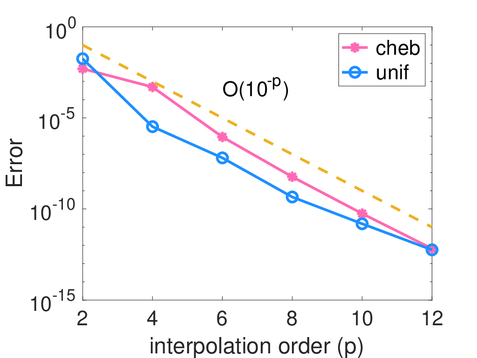
Fig. 5 shows the (relative) error of evaluating Eq. 1 as a function of , where the kernel functions are and , respectively. The error is defined as
where stands for the approximation constructed implicitly in PBBFMM3D. Since both kernel functions are analytic (away from the origin), the error of our interpolation using either Chebyshev nodes or uniform nodes decays exponentially.
Fig. 5 shows the scaling of the sequential running time with respect to the number of points . We see that the time increases linearly as increases, as opposed to the quadratic increase of evaluating Eq. 1 naively.

4.2 Parallel scalability
In this section, we present the parallel running time of PBBFMM3D on up to 32 cores. We focus on the kernel function and use Chebyshev nodes in Definition 2.3 with . Table 1 reports the parallel running time. To show the parallel scalability, we chose the number of cores to be a power of 2. But that is not required in PBBFMM3D. The baseline (1 core) is the serial version used in [18, 9]. As the table shows, we obtained approximately speedup on 32 cores for .
| Time (seconds) | ||||||
|---|---|---|---|---|---|---|
| 1 core | 2 cores | 4 cores | 8 cores | 16 cores | 32 cores | |
| e+4 | e+0 | e+0 | e+0 | e-1 | e-1 | e-1 |
| e+4 | e+1 | e+1 | e+1 | e+0 | e+0 | e+0 |
| e+4 | e+2 | e+2 | e+2 | e+1 | e+1 | e+1 |
Fig. 6(a) shows the strong scalability of PBBFMM3D, i.e., the running time using a sequence of increasing number of cores for a fixed problem size. We provided a breakdown of the running time into the four stages: upward pass, far-field interaction, downward pass, and near-field interaction. We see that the running time for all stages nearly halved as the number of cores doubled.
Fig. 6(b) shows the weak scalability of PBBFMM3D, i.e., the running time for a fixed problem size per core. So we increased the number of particles proportionally to the number of cores. As the figure shows, the time spent on each stage in the FMM only increased by a small amount when the problem size increased by (the number of cores also increased by ). The ideal runtime would stay unchanged due to the linear complexity of PBBFMM3D. Our implementation achieved an efficiency of 73% to 86% (serial time/parallel time).

4.3 Application in Gaussian Processes
Gaussian random field (GRF) theory [35, 36] has been widely used in interpolation and estimation of spatially correlated unknowns. For example, GRF methods can be used for estimating the permeability of the underground soil and rock, which is of critical interest to hydrogeologists and petroleum engineers [37, 38]. In GRF methods, a covariance matrix is required as the prior information of the underlying unknown field. However, practical applications typically require large numbers of unknowns, so dimension reduction techniques such as the principle component analysis are required.
To obtain the top- principle components, we employ PBBFMM3D to compute the truncated eigenvalue decomposition of the covariance matrix. In particular, we use a randomized method (Algorithm 5.3 in [39]) to calculate the top- eigenvalues and their associated eigenvectors, and the randomized algorithm requires evaluating Eq. 1 times (same target and source points but with different weights). While the original method requires operations, we accelerate the method with PBBFMM3D and arrive at the optimal complexity, where is the number of data points.
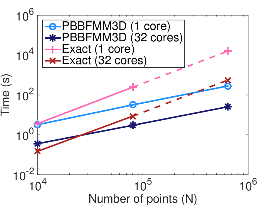
In the next experiment, we randomly generated data points in the unit cube and employed the kernel function , one-dimensional Matérn kernel with smoothness 1/2. The goal was to compute the top-100 eigen-pairs of the covariance matrix, where 120 matrix-vector products (packed into one matrix-matrix product) were evaluated twice in the randomized algorithm. In the original randomized method, matrix-matrix products are computed by calling the dgemm subroutine in the Intel MKL library (with multi-threading on 32 cores). In the PBBFMM3D-accelerated method, the number of Chebyshev nodes was , and the number of tree levels were 3, 4 and 5 for the three increasing problem sizes. We measured the error , where and are the eigenvalues computed using the original method and the PBBFMM3D-accelerated method, respectively. The errors for and are and , respectively.
Fig. 7 shows the running time of the original method and our accelerated method. In Geostatistics applications, the original randomized method with exact matrix-matrix products is the common practice, and therefore we set that as our baseline. This allows us to show the best speedup and scaling one can achieve from leveraging PBBFMM3D. In the original method, we need to evaluate all entries of the covariance matrix and compute matrix-matrix products, both of which scale as . It is worth noting that when , forming the entire covariance matrix requires 3.2 TB of memory.
In the PBBFMM3D-accelerated method, we need to evaluate only entries of the covariance matrix. As Fig. 7 shows, our method scales linearly with respect to the problem size , and thus the speedup over the original method becomes more pronounced when increases.
In the last experiment, we apply PBBFMM3D to data points lying on an unstructured grid, as shown in Figure 8. Same as above, we compute the top-50 eigenvectors with the randomized algorithm accelerated by PBBFMM3D. For this experiment, we employ the kernel function , and we used Chebyshev nodes in PBBFMM3D.

5 Conclusions
We have introduced PBBFMM3D, a black-box algorithm/software for evaluating kernel matrix-vector multiplication on shared-memory machines. The target kernels are non-oscillatory translation invariant functions that are sufficiently smooth away from the origin. The user needs only provide a function routine that returns the kernel value given a source point and a target point, if the kernel function is not already implemented. (The user can also specify the degree of homogeneity and whether the kernel is symmetric or skew-symmetric to active specific optimizations.) Our algorithm requires memory and work, where is the number of data points.
A parallel algorithm is presented in this paper and implemented using OpenMP for shared-memory machines. We have presented parallel scalability results on up to 32 cores and achieved at most speedup. We have also presented an application in geostatistics, where we accelerated the computation of the truncated eigen-decomposition of covariance matrices.
References
- [1] A. G. Gray, A. W. Moore, N-body’problems in statistical learning, in: Advances in neural information processing systems, 2001, pp. 521–527.
- [2] T. Hofmann, B. Schölkopf, A. J. Smola, Kernel methods in machine learning, The annals of statistics (2008) 1171–1220.
- [3] S. Ambikasaran, A. K. Saibaba, E. F. Darve, P. K. Kitanidis, Fast algorithms for Bayesian inversion, in: Computational Challenges in the Geosciences, Springer, 2013, pp. 101–142.
- [4] J. Y. Li, S. Ambikasaran, E. F. Darve, P. K. Kitanidis, A Kalman filter powered by H2-matrices for quasi-continuous data assimilation problems, Water Resources Research 50 (5) (2014) 3734–3749.
- [5] L. Greengard, V. Rokhlin, A fast algorithm for particle simulations, Journal of computational physics 73 (2) (1987) 325–348.
- [6] L. Greengard, V. Rokhlin, A new version of the fast multipole method for the Laplace equation in three dimensions, Acta numerica 6 (1997) 229–269.
- [7] R. Simpson, Z. Liu, Acceleration of isogeometric boundary element analysis through a black-box fast multipole method, Engineering Analysis with Boundary Elements 66 (2016) 168–182.
- [8] D. Zhao, J. Huang, Y. Xiang, Fast multipole accelerated boundary integral equation method for evaluating the stress field associated with dislocations in a finite medium, Communications in Computational Physics 12 (1) (2012) 226–246.
- [9] C. Chen, S. Aubry, T. Oppelstrup, A. Arsenlis, E. Darve, Fast algorithms for evaluating the stress field of dislocation lines in anisotropic elastic media, Modelling and Simulation in Materials Science and Engineering (2018).
- [10] D. Alfke, D. Potts, M. Stoll, T. Volkmer, NFFT meets Krylov methods: Fast matrix-vector products for the graph Laplacian of fully connected networks, Frontiers in Applied Mathematics and Statistics 4 (2018) 61.
- [11] D. Ruiz-Antolin, A. Townsend, A nonuniform fast Fourier transform based on low rank approximation, SIAM Journal on Scientific Computing 40 (1) (2018) A529–A547.
- [12] Y. Fu, K. J. Klimkowski, G. J. Rodin, E. Berger, J. C. Browne, J. K. Singer, R. A. Van De Geijn, K. S. Vemaganti, A fast solution method for three-dimensional many-particle problems of linear elasticity, International Journal for Numerical Methods in Engineering 42 (7) (1998) 1215–1229.
- [13] Y. Fu, G. J. Rodin, Fast solution method for three-dimensional Stokesian many-particle problems, International Journal for Numerical Methods in Biomedical Engineering 16 (2) (2000) 145–149.
- [14] L. F. Greengard, J. Huang, A new version of the fast multipole method for screened Coulomb interactions in three dimensions, Journal of Computational Physics 180 (2) (2002) 642–658.
- [15] K.-i. Yoshida, N. Nishimura, S. Kobayashi, Application of fast multipole Galerkin boundary integral equation method to elastostatic crack problems in 3d, International Journal for Numerical Methods in Engineering 50 (3) (2001) 525–547.
- [16] A. Dutt, M. Gu, V. Rokhlin, Fast algorithms for polynomial interpolation, integration, and differentiation, SIAM Journal on Numerical Analysis 33 (5) (1996) 1689–1711.
- [17] Z. Gimbutas, V. Rokhlin, A generalized fast multipole method for nonoscillatory kernels, SIAM Journal on Scientific Computing 24 (3) (2003) 796–817.
- [18] W. Fong, E. Darve, The black-box fast multipole method, Journal of Computational Physics 228 (23) (2009) 8712–8725.
- [19] L. Ying, G. Biros, D. Zorin, A kernel-independent adaptive fast multipole algorithm in two and three dimensions, Journal of Computational Physics 196 (2) (2004) 591–626.
- [20] P.-G. Martinsson, V. Rokhlin, An accelerated kernel-independent fast multipole method in one dimension, SIAM Journal on Scientific Computing 29 (3) (2007) 1160–1178.
- [21] D. Malhotra, G. Biros, PVFMM: A parallel kernel independent FMM for particle and volume potentials, Communications in Computational Physics 18 (3) (2015) 808–830.
- [22] C. D. Yu, J. Levitt, S. Reiz, G. Biros, Geometry-oblivious FMM for compressing dense SPD matrices, in: Proceedings of the International Conference for High Performance Computing, Networking, Storage and Analysis, ACM, 2017, p. 53.
- [23] J. Lee, A. Kokkinaki, P. K. Kitanidis, Fast large-scale joint inversion for deep aquifer characterization using pressure and heat tracer measurements, Transport in Porous Media 123 (2018) 533–543.
- [24] A. Verde, A. Ghassemi, et al., Efficient solution of large-scale displacement discontinuity problems using the fast multipole method, in: 47th US Rock Mechanics/Geomechanics Symposium, American Rock Mechanics Association, 2013.
- [25] A. Verde, A. Ghassemi, Fast multipole displacement discontinuity method (FM-DDM) for geomechanics reservoir simulations, International Journal for Numerical and Analytical Methods in Geomechanics 39 (18) (2015) 1953–1974.
- [26] M. Farmahini-Farahani, A. Ghassemi, Simulation of micro-seismicity in response to injection/production in large-scale fracture networks using the fast multipole displacement discontinuity method (FMDDM), Engineering Analysis with Boundary Elements 71 (2016) 179–189.
- [27] P. Coulier, H. Pouransari, E. Darve, The inverse fast multipole method: using a fast approximate direct solver as a preconditioner for dense linear systems, SIAM Journal on Scientific Computing 39 (3) (2017) A761–A796.
- [28] T. Takahashi, C. Chen, E. Darve, Parallelization of the inverse fast multipole method with an application to boundary element method, Computer Physics Communications 247 (2020) 106975.
- [29] E. Agullo, B. Bramas, O. Coulaud, E. Darve, M. Messner, T. Takahashi, Task-based FMM for multicore architectures, SIAM Journal on Scientific Computing 36 (1) (2014) C66–C93.
- [30] M. S. Warren, J. K. Salmon, Astrophysical N-body simulations using hierarchical tree data structures, SC 92 (1992) 570–576.
- [31] M. S. Warren, J. K. Salmon, A parallel hashed oct-tree n-body algorithm, in: Proceedings of the 1993 ACM/IEEE conference on Supercomputing, 1993, pp. 12–21.
- [32] T. Takahashi, C. Cecka, E. Darve, Optimization of the parallel black-box fast multipole method on CUDA, in: 2012 Innovative Parallel Computing (InPar), IEEE, 2012, pp. 1–14.
- [33] E. Agullo, B. Bramas, O. Coulaud, E. Darve, M. Messner, T. Takahashi, Task-based FMM for heterogeneous architectures, Concurrency and Computation: Practice and Experience 28 (9) (2016) 2608–2629.
- [34] L. N. Trefethen, Approximation theory and approximation practice, Siam, 2013.
- [35] C. E. Rasmussen, C. K. I. Williams, Gaussian Processes for Machine Learning (Adaptive Computation and Machine Learning), The MIT Press, 2005.
- [36] M. L. Stein, Interpolation of spatial data : some theory for kriging, Springer series in statistics, Springer, New York, 1999.
- [37] P. K. Kitanidis, Introduction to geostatistics: applications in hydrogeology, Cambridge University Press, 1997.
- [38] D. S. Oliver, A. C. Reynolds, N. Liu, Inverse theory for petroleum reservoir characterization and history matching, Cambridge University Press, 2008.
- [39] N. Halko, P.-G. Martinsson, J. A. Tropp, Finding structure with randomness: Probabilistic algorithms for constructing approximate matrix decompositions, SIAM review 53 (2) (2011) 217–288.
- [40] M. S. Alnæs, J. Blechta, J. Hake, A. Johansson, B. Kehlet, A. Logg, C. Richardson, J. Ring, M. E. Rognes, G. N. Wells, The FEniCS project version 1.5, Archive of Numerical Software 3 (100) (2015). doi:10.11588/ans.2015.100.20553.