Why Learning of Large-Scale Neural Networks Behaves Like Convex Optimization

Based on the universal approximation theorems in Cybenko 1989; Hornik et al. 1989; Hornik 1991, any function in $L^{1}(\mathbb{U}_{K})$ can be approximated up to arbitrary precision by a well-structured neural network of sufficiently large model size. Here, we use $\Lambda_{M}$ to represent the set of all well-structured neural networks using $M$ free model parameters, and all weight parameters of each neural network are denoted as a vector $\mathbf{w}$ ($\mathbf{w}\in\mathbb{R}^{M}$). Obviously, if $M$ is made sufficiently large, $\Lambda_{M}$ is a good choice to parameterize the function space $L^{1}(\mathbb{U}_{K})$ because given any bounded function $f(\mathbf{x})\in L^{1}(\mathbb{U}_{K})$, there exists at least one set of model parameters in $\Lambda_{M}$, denoted as $\mathbf{w}$, to make the corresponding neural network approximate $f(\mathbf{x})$ up to arbitrary precision. In this case, the function represented by the underlying neural network is denoted as $f_{\mathbf{w}}(\mathbf{x})$. Furthermore, if $M$ is finite and all model parameters are bounded, every function represented by each possible neural network in $\Lambda_{M}$ belongs to $L^{1}(\mathbb{U}_{K})$. As a result, once we pre-determine the neural network structure of model size $M=|\mathbf{w}|$ (assume that $M$ is sufficiently large), the functional minimization problem in eq.(2) can be simplified into an equivalent parameter optimization problem as follows:

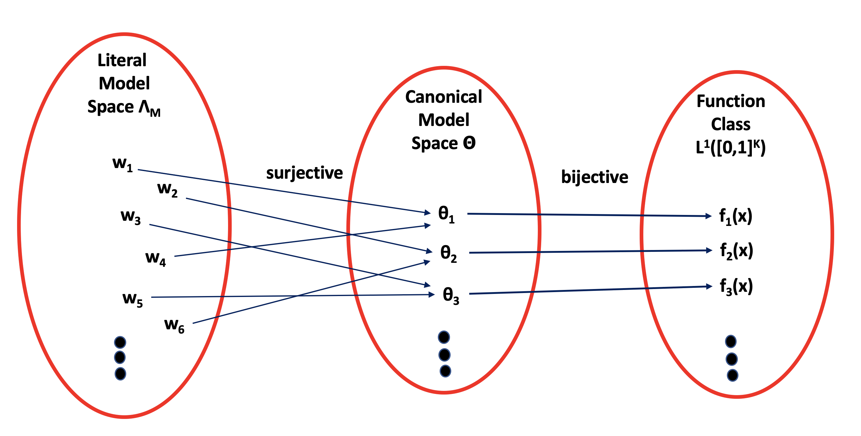
However, due to the weight-space symmetries and network redundancy, the mapping from $\Lambda_{M}$ to $L^{1}(\mathbb{U}_{K})$ is surjective but not injective. For any function $f\in L^{1}(\mathbb{U}_{K})$, there always exist many different $\mathbf{w}$ in $\Lambda_{M}$ to make neural networks represent $f$ equally well. In this work, the space of neural networks, $\Lambda_{M}$, is called literal model space of $L^{1}(\mathbb{U}_{K})$ because it only satisfies the existence requirement but not the uniqueness one. It is the non-uniqueness of $\Lambda_{M}$ that makes it extremely difficult to directly conduct the theoretical analysis for the optimization problem in eq.(3).

Here, let’s consider the so-called canonical model space for $L^{1}(\mathbb{U}_{K})$. A model space is called to be canonical if it satisfies both existence and uniqueness requirements. In other words, for every function $f\in L^{1}(\mathbb{U}_{K})$, there exists exactly one unique model in the canonical model space to represent $f$. Moreover, every model in the canonical model space corresponds to a unique function in $L^{1}(\mathbb{U}_{K})$. Therefore, the mapping between $L^{1}(\mathbb{U}_{K})$ and its canonical model space is bijective. For $L^{1}(\mathbb{U}_{K})$, the multivariate Fourier series naturally form such a canonical model space for $L^{1}(\mathbb{U}_{K})$.

As in Pinsky 2002, given any function $f(\mathbf{x})\in L^{1}(\mathbb{U}_{K})$, we may compute its multivariate Fourier coefficients as follows:

where $i=\sqrt{-1}$ and $\theta_{\boldsymbol{k}}\in\mathbb{C}$, and $\boldsymbol{k}=[k_{1},k_{2},\cdots,k_{K}]$ is a tuple of $K$ integers, denoting the $K$-dimensional index of each Fourier coefficient. All Fourier coefficients of a function $f(\mathbf{x})$ can be arranged as an infinite sequence, i.e. $\boldsymbol{\theta}=\{\theta_{\boldsymbol{k}}\;|\;\boldsymbol{k}\in\mathbb{Z}^{K}\}$, which in turn can be viewed as a point in a Hilbert space with an infinite number of dimensions. This Hilbert space is denoted as $\boldsymbol{\Theta}$. For the notational simplicity, we may represent eq.(4) by a generic mapping from any $f(\mathbf{x})\in L^{1}(\mathbb{U}_{K})$ to a $\boldsymbol{\theta}\in\boldsymbol{\Theta}$ as: $\boldsymbol{\theta}:={\mathscr{F}}\big(f(\mathbf{x})\big).$

According to the Fourier theorem, for any function $f(\mathbf{x})\in L^{1}(\mathbb{U}_{K})$, these Fourier coefficients may be used to perfectly reconstruct $f(\mathbf{x})$ by summing the following Fourier series, which converges everywhere in $\mathbf{x}\in\mathbb{U}_{K}$:

Because both eq.(4) and eq.(5) converge for any function $f(\mathbf{x})\in L^{1}(\mathbb{U}_{K})$, therefore, $\boldsymbol{\Theta}$ is a canonical model space of $L^{1}(\mathbf{x})$. Every function in $f(\mathbf{x})$ can be uniquely represented by all of its Fourier coefficients $\boldsymbol{\theta}$ in $\boldsymbol{\Theta}$.

According to the Riemann-Lebesgue lemma (pp.18 in Pinsky 2002), the Fourier coefficients $\theta_{\boldsymbol{k}}$ decay from both sides in every dimension of $\boldsymbol{k}$, i.e., $|\theta_{\boldsymbol{k}}|\to 0$ as the absolute value of any dimension of $\boldsymbol{k}$ goes to infinity, $\max|\boldsymbol{k}|\to\infty$. As a result, the Fourier serie in eq.(5) can be truncated into a partial sum centered at the origin. Given any small number $\epsilon>0$, for any function $f(\mathbf{x})\in L^{1}(\mathbb{U}_{K})$, we can always choose a finite number of the most significant Fourier coefficients located in the center, which are denoted as ${\cal N}_{\epsilon}:=\{\boldsymbol{k}\,\mid\,|k_{1}|\leq N_{1},\cdots,|k_{K}|\leq N_{K}\}$. The cardinality of ${\cal N}_{\epsilon}$ is denoted as $N=|{\cal N}_{\epsilon}|$. The truncated Fourier coefficients can also be arranged onto an $N$-dimensional vector, $\boldsymbol{\theta}_{\epsilon}=\{\theta_{\boldsymbol{k}}\,\mid\,\boldsymbol{k}\in{\cal N}_{\epsilon}\}$, which may be viewed as a point in a complete normed linear space with $N$ dimensions. This finite-dimensional normed linear space is thus denoted as $\boldsymbol{\Theta}_{\epsilon}$. Moreover, we may use these truncated coefficients in ${\cal N}_{\epsilon}$ to form a partial sum to approximate the original function $f(\mathbf{x})$ up to the precision $1-\epsilon^{2}$:

where $\hat{f}(\mathbf{x})$ is an infinitely differentiable function in $\mathbb{U}_{K}$, approximating $f(\mathbf{x})$ up to $1-\epsilon^{2}$ in the $L^{2}$ norm, i.e. $\idotsint_{\mathbf{x}\in\mathbb{U}_{K}}\;\|f(\mathbf{x})-\hat{f}(\mathbf{x})\|^{2}d\mathbf{x}\leq\epsilon^{2}$.

In summary, for any function $f(\mathbf{x})\in L^{1}(\mathbb{U}_{K})$, we may calculate its Fourier coefficients as in eq.(4) to represent it uniquely in the infinite-dimensional canonical space $\boldsymbol{\Theta}$ as $\boldsymbol{\theta}={\mathscr{F}}\left(f(\mathbf{x})\right)$ where $\boldsymbol{\theta}\in\boldsymbol{\Theta}$. Furthermore, for the computational convenience, we may approximate $\boldsymbol{\Theta}$ with a finite-dimension space up to any arbitrary precision. For a given tolerance error $\epsilon$, we may truncate $\boldsymbol{\theta}$ by leaving out all insignificant coefficients and construct $\boldsymbol{\theta}_{\epsilon}$ of $N$ dimensions as above. This process is conveniently denoted as a mapping: $\boldsymbol{\theta}_{\epsilon}={\mathscr{F}}_{\epsilon}(f(\mathbf{x}))$. On the other hand, $\boldsymbol{\theta}_{\epsilon}$ may be used to construct $\hat{f}(\mathbf{x})$ based on the partial sum in eq. (6), i.e. $\hat{f}(\mathbf{x})={\mathscr{F}}^{-1}(\mathbf{x}|\boldsymbol{\theta}_{\epsilon})$. As shown above, $\hat{f}(\mathbf{x})$ approximates the original function $f(\mathbf{x})$ up to the precision $1-\epsilon^{2}$, denoted as $\hat{f}(\mathbf{x})=f(\mathbf{x})+O(\epsilon)$. Here, we call this finite dimensional space $\boldsymbol{\Theta}_{\epsilon}$ as an $\epsilon$-precision canonical model space of $L^{1}(\mathbb{U}_{K})$. Obviously, the approximation error $\epsilon^{2}$ can be made arbitrarily small so as to make $\boldsymbol{\Theta}_{\epsilon}$ approach $\boldsymbol{\Theta}$ as much as possible.

For any neural network in the literal model space $\Lambda_{M}$, assuming its model parameter is $\mathbf{w}^{(0)}$, it forms a function $f_{\mathbf{w}^{(0)}}(\mathbf{x})$ between its input and output. As we know $f_{\mathbf{w}^{(0)}}(\mathbf{x})\in L^{1}(\mathbb{U}_{K})$, we can easily find its corresponding representation in the canonical model space with infinite dimensions via $\boldsymbol{\theta}^{(0)}={\mathscr{F}}(f_{\mathbf{w}^{(0)}}(\mathbf{x}))$, where $\boldsymbol{\theta}^{(0)}\in\boldsymbol{\Theta}$. Similarly, we may truncate $\boldsymbol{\theta}^{(0)}$ to find its representation in an $\epsilon$-precision canonical model space with $N$ dimensions as $\boldsymbol{\theta}_{\epsilon}^{(0)}={\mathscr{F}}_{\epsilon}(f_{\mathbf{w}^{(0)}}(\mathbf{x}))$, where $\boldsymbol{\theta}^{(0)}_{\epsilon}\in\boldsymbol{\Theta}_{\epsilon}$. As shown in Figure 1, the mapping from $\Lambda_{M}$ to $\boldsymbol{\Theta}$ is surjective but not injective while the mapping from $\boldsymbol{\Theta}$ to $L^{1}(\mathbb{U}_{K})$ is bijective.

Let’s consider the original learning problem eq.(2) in the canonical model space. Since canonical model spaces normally have nice structures, i.e., every $f(\mathbf{x})$ is uniquely represented as a linear combination of some fixed orthogonal base functions. The functional minimization in eq.(2) turns to be an optimization problem to determine the unknown coefficients in a linear combination as follows:

This learning problem turns out to be strikingly easy in the canonical model space.

Proof: Given an arbitrarily small tolerance error $\epsilon\geq 0$, any function $f(\mathbf{x})\in L^{1}(\mathbb{U}_{K})$ can be uniquely mapped to a point in an canonical space $\boldsymbol{\Theta}_{\epsilon}$ as: $\boldsymbol{\theta}_{\epsilon}={\mathscr{F}}_{\epsilon}(f(\mathbf{x}))$. Meanwhile, the function $f(\mathbf{x})$ may be approximated by $\boldsymbol{\theta}_{\epsilon}=\{\boldsymbol{k}\mid\boldsymbol{k}\in{\cal N}_{\epsilon}\}$ with the partial sum of Fourier series: $f_{\boldsymbol{\theta}_{\epsilon}}(\mathbf{x})=\sum_{\boldsymbol{k}\in{\cal N}_{\epsilon}}\;\theta_{\boldsymbol{k}}\;e^{2\pi i\boldsymbol{k}\cdot\mathbf{x}}=\sum_{\boldsymbol{k}\in{\cal N}_{\epsilon}}\;\theta_{\boldsymbol{k}}\eta_{\boldsymbol{k}}(\mathbf{x}),$ where $\eta_{\boldsymbol{k}}(\mathbf{x})=e^{2\pi i\boldsymbol{k}\cdot\mathbf{x}}$. If we constrain to optimize eq.(2) in the canonical space $\boldsymbol{\Theta}_{\epsilon}$, the objective function is represented as:

Since the loss measure $l(\cdot)$ itself is a convex function of its second argument, and the argument is a linear combination of all parameters $\theta_{\boldsymbol{k}}$, therefore, the right-hand side of the above equation is a convex function of its parameter $\boldsymbol{\theta}_{\epsilon}$. When mean squared error is used for $l(\cdot)$, the above procedure is the same as the well-known least square method.

Due to eq.(1), if a global minimum $\boldsymbol{\theta}^{*}_{\epsilon}$ achieves zero loss, it must satisfy: $l\left(y_{i},f(\mathbf{x}_{i})\right)=l\left(y_{i},\sum_{\boldsymbol{k}\in{\cal N}_{\epsilon}}\theta_{\boldsymbol{k}}\eta_{\boldsymbol{k}}(\mathbf{x}_{i})\right)=0\;(i=1,2,\cdots,T)$, which are equivalent to a system of $T$ linear equations: $\sum_{\boldsymbol{k}\in{\cal N}_{\epsilon}}\theta_{\boldsymbol{k}}\eta_{\boldsymbol{k}}(\mathbf{x}_{i})=y_{i}\;(i=1,2,\cdots,T).$

Obviously, if the dimensionality of the canonical model space is not less than the number of point-wise distinct (and noncontradictory) training samples, $T$, we have more free variables in $\boldsymbol{\theta}^{*}_{\epsilon}$ than the total number of linear equations. Therefore, there exists at least one solution to jointly satisfy these independent equations, which also achieves the zero loss at the same time. If the dimensionality of the canonical model space is equal to the number of point-wise distinct training samples, there exists a unique global minimum that achieves zero loss. $\hskip 0.0pt{\hfill\blacksquare}$

Proof: For any two functions, $f_{1},f_{2}\in L^{1}(\mathbb{U}_{K})$, we may map them into the canonical model space $\boldsymbol{\Theta}$ to find their representations as: $\boldsymbol{\theta}_{1}={\mathscr{F}}(f_{1})$ and $\boldsymbol{\theta}_{2}={\mathscr{F}}(f_{2})$. As shown in eq.(5), both $f_{1}$ and $f_{2}$ can be represented as a linear function of $\boldsymbol{\theta}_{1}$ and $\boldsymbol{\theta}_{2}$. Since $l(\cdot)$ is a convex function, for any $0\leq\varepsilon\leq 1$, it is trivial to show that $Q(\varepsilon\,f_{1}+(1-\varepsilon)\,f_{2}|\mathcal{D}_{T})\leq\varepsilon\,Q(f_{1}|\mathcal{D}_{T})+(1-\varepsilon)\,Q(f_{2}|\mathcal{D}_{T}).$ Therefore, $Q(f|\mathcal{D}_{T})$ is a convex functional in $L^{1}(\mathbb{U}_{K})$. $\hskip 0.0pt{\hfill\blacksquare}$

As shown above, learning in the canonical model space is a standard convex optimization problem. However, the direct learning in the canonical model space may be computationally prohibitive in high-dimensional canonical spaces. At present, the common practice in machine learning is still to learn neural networks in the literal model space. Here we will look at how the canonical space may help to understand the learning behaviours of neural networks in the literal space.

The learning of neural networks mainly uses the first-order methods, which solely rely on the gradients of the objective function. We will first investigate how the gradients in the literal model space are related to the gradients in the canonical model space. Given model parameters $\mathbf{w}$ of a neural network, which may be viewed as a point in the literal space $\Lambda_{M}$ with $M=|\mathbf{w}|$ dimensions, the objective function at $\mathbf{w}$ is denoted as $Q(f_{\mathbf{w}}|\mathcal{D}_{T})$. If the training set $\mathcal{D}_{T}$ has $T$ point-wise distint training samples, we consider an $\epsilon$-precision canonical space, $\boldsymbol{\Theta}_{\epsilon}$. The cardinality of $\boldsymbol{\Theta}_{\epsilon}$, denoted as $N$, is chosen to satisfy two conditions: i) $N$ is not smaller than $T$; ii) $N$ is large enough to make the truncation error $\epsilon$ sufficiently small. In this way, for any $\mathbf{w}$ in $\Lambda_{M}$, it may be mapped to this canonical space as $\boldsymbol{\theta}_{\epsilon}=\mathscr{F}_{\epsilon}(f_{\mathbf{w}}(\mathbf{x}))$ ($\boldsymbol{\theta}_{\epsilon}\in\boldsymbol{\Theta}_{\epsilon}$). Obviously, $Q(f_{\mathbf{w}}|\mathcal{D}_{N})=Q(\boldsymbol{\theta}|\mathcal{D}_{T})+O(\epsilon)$. However, the residual error term may be ignored since it can be made arbitrarily small when we choose a large enough $N$. Moreover, due to $N\geq T$, the global minimum of the objective function achieves zero loss in this canonical space. In this work, we consider the learning problem of over-parameterized neural networks, where the dimensionality of the literal space, $M=|\mathbf{w}|$, is much larger than the dimensionality of this canonical space, namely $M\gg N$.

Based on the chain rule, we have:

which can be represented as the following matrix format:

where the $M\times N$ matrix is called disparity matrix, denoted as $\mathbf{H}(\mathbf{w})$. The disparity matrix $\mathbf{H}(\mathbf{w})$ is composed of $M$ sets of Fourier coefficients (computed over the input $\mathbf{x}$) of partial derivatives of the neural network function with respect to each of its weights. When we form the $m$-th row of the disparity matrix, we first compute the partial derivative of the neural network function $f_{\mathbf{w}}(\mathbf{x})$ with respect to $m$-th parameter, $w_{m}$, in the neural netowork. This partial derivative, $\frac{\partial f_{\mathbf{w}}(\mathbf{x})}{\partial{w}_{m}}$, is still a function of input $\mathbf{x}$. Then we first apply Fourier series in eq.(5) to it and then truncate to keep the total $N$ most significant Fourier coefficients. These $N$ coefficients are aligned to be placed in the $m$-th row of the disparity matrix $\mathbf{H}(\mathbf{w})$. This process is repeated for every parameter of the neural network so as to fill up all rows in the $M\times N$ matrix. Obviously, the disparity matrix depends on $\mathbf{w}$ because when $\mathbf{w}$ take different values, these function derivatives are normally different and so are their Fourier coefficients. For any given neural network $\mathbf{w}$, this mapping can be represented as a compact matrix format:

From the above, we can see that the gradient in the literal space is related to its corresponding gradient in the canonical space through a linear transformation at every $\mathbf{w}$, which is represented by the disparity matrix $\mathbf{H}(\mathbf{w})$. The disparity matrix varies when $\mathbf{w}$ moves from one model to another in the literal space. As a result, we say that the gradient in the literal space is linked to its corresponding gradient in the canonical space via a point-wise linear transformation.

Proof: If $\mathbf{w}^{*}$ is a stationary point, it implies that the gradient vanishes at $\mathbf{w}^{*}$ in the literal model space, i.e., $\Big[\nabla_{\mathbf{w}}Q(\mathbf{w}^{*})\Big]_{M\times 1}=0$. Substituting this into eq.(9), we have

because $M\geq N$ and $\mathbf{H}(\mathbf{w}^{*})$ has the full rank ($N$), the only solution to the above equations in the canonical space is $\nabla_{\boldsymbol{\theta}_{\epsilon}}Q(\boldsymbol{\theta}^{*}_{\epsilon})=0$. In other words, the corresponding model $\boldsymbol{\theta}^{*}_{\epsilon}$ in the canonical space is also a stationary point. Since $Q(\boldsymbol{\theta}_{\epsilon})$ is a convex function in the canonical space, this implies the corresponding model $\boldsymbol{\theta}^{*}$ is a global minimum. Due to the fact that the objective functions are equal across two spaces when we map $\mathbf{w}^{*}$ to $\boldsymbol{\theta}^{*}_{\epsilon}$, i.e., $Q(\mathbf{w}^{*})=Q(\boldsymbol{\theta}^{*}_{\epsilon})$, we conclude that $\mathbf{w}^{*}$ is also a global minimum in the literal space. $\hskip 0.0pt{\hfill\blacksquare}$

Proof: The disparity matrix is an $M\times N$ matrix and we still assume $M\geq N$. If $\mathbf{H}(\mathbf{w}^{(0)})$ degenerates and does not have full rank at $\mathbf{w}^{(0)}$, it is possible to have zero or some nonzero solutions in the canonical space to the system of under-specified equations in eq.(10). For the zero solution $\nabla_{\boldsymbol{\theta}_{\epsilon}}Q(\boldsymbol{\theta}_{\epsilon}^{(0)})=0$, the corresponding model of $\boldsymbol{\theta}_{\epsilon}^{(0)}$ in literal space is a global minimum because the objective function is convex in the canonical space. However, for the non-zero solutions, $\nabla_{\boldsymbol{\theta}_{\epsilon}}Q(\boldsymbol{\bar{\theta}}_{\epsilon}^{(0)})\neq 0$, the corresponding model of $\boldsymbol{\bar{\theta}}_{\epsilon}^{(0)}$ in literal space is certainly not a global minimum since the gradient does not vanish in the canonical space. They may correspond to some saddle points in the literal space since the gradient vanishes only in the literal space, or some flat regions of the loss surface where the disparity matrix $\mathbf{H}(\mathbf{w}^{(0)})=0$. As these models must correspond to a point in the canonical space, if it is not located in a flat region, it can not be a local minimum since it must have a direction to decrease the loss function. Otherwise, it must correspond to the global minimum in the canonical space. $\hskip 0.0pt{\hfill\blacksquare}$

As we know that neural networks are directly learned in the literal space as in eq.(3). We normally use some fairly simple first-order local search methods to solve this non-convex optimization problem. These methods include gradient descent (GD) and more computationally efficient stochastic gradient descent (SGD) algorithms. As shown in Algorithm 1, these algorithms operate in a pretty simple fashion: it starts from a random model and the model is iteratively updated with the currently computed gradient $\nabla_{\mathbf{w}}Q(\mathbf{w}^{(k)})$ and some preset step sizes, $h_{k}\;(k=0,1,2,\cdots)$, which are usually decaying.

The optimization in eq.(3) is clearly non-convex in the literal space for any nonlinear neural networks. However, due to the fact that both literal and canonical spaces are complete and the gradients in both spaces are linked through a point-wise linear transformation, in the following, we will theoretically prove that the gradient descent methods can solve this non-convex problem efficiently in the literal space in a similar way as solving normal convex optimization problems. As long as some minor conditions hold, the gradient descent methods surely converge to a global minimum even in the literal space.

Proof: In non-convex optimization problems, as long as the objective function satisfies the Liptschitz condition and the step sizes are small enough at each step, the gradient descent in Algorithm 1 is guaranteed to converge to a stationary point, namely $\|\nabla_{\mathbf{w}}Q(\mathbf{w}^{(k)})\|\to 0$ as $k\to\infty$ (Nesterov 2004). As long as $\mathbf{H}(\mathbf{w}^{(k)})$ maintains full rank, according to Lemma 1, $\mathbf{w}^{(k)}$ approaches a global minimum, i.e. $Q(\mathbf{w}^{(k)})\to 0$ as $k\to\infty$.

Moreover, as shown in eq.(9), we have $\nabla_{\mathbf{w}}Q(\mathbf{w}^{(k)})=\mathbf{H}(\mathbf{w}^{(k)})\,\nabla_{\boldsymbol{\theta}}Q(\boldsymbol{\theta}^{(k)})$ for $k=0,1,\cdots$, where $\boldsymbol{\theta}^{(k)}$ denotes the corresponding representation of $\mathbf{w}^{(k)}$ in the canonical space. As $\nabla_{\mathbf{w}}Q(\mathbf{w}^{(k)})\to 0$, $\mathbf{H}(\mathbf{w}^{(k)})$ normally does not approach 0. Let us show this by contradiction. Assume $\mathbf{H}(\mathbf{w}^{(k)})\to 0$, which means that every row of $\mathbf{H}(\mathbf{w}^{(k)})$ approaches 0 at the same time. As we know, $m$-th row of $\mathbf{H}(\mathbf{w})$ corresponds to the Fourier series coefficients of the function $\frac{\partial f_{\mathbf{w}}(\mathbf{x})}{\partial{w}_{m}}$. If the Fourier coefficients are all approaching zero, it means that the function itself approaches 0 as well, i.e., $\frac{\partial f_{\mathbf{w}}(\mathbf{x})}{\partial{w}_{m}}=0$. It means the current neural network function $f_{\mathbf{w}}(\mathbf{x})$ is irrelevant to the weight ${w}_{m}$. We may simply remove the link associated to ${w}_{m}$ without changing $f_{\mathbf{w}}(\mathbf{x})$. Because all rows of $\mathbf{H}(\mathbf{w})$ approaches 0, we may remove all links of all weights from the neural network without changing $f_{\mathbf{w}}(\mathbf{x})$. In other words, the current model is located at a locally flat region of the loss function surface. The rank of the disparity matrix $\mathbf{H}(\mathbf{w}^{(k)})$ is zero in the flat region. Therefore, if all $\mathbf{H}(\mathbf{w}^{(k)})$ maintain full rank at the same time, as $\nabla_{\mathbf{w}}Q(\mathbf{w}^{(k)})\to 0$, we will surely have $\nabla_{\boldsymbol{\theta}}Q(\boldsymbol{\theta}^{(k)})\to 0$. The trajectory of $\theta^{(k)}$ will converge towards a global minimum in the convex loss surface in the canonical space. Since the objective functions are equal across two spaces when we map $\mathbf{w}^{(k)}$ to $\boldsymbol{\theta}^{(k)}$, i.e., $Q(\mathbf{w}^{(k)})=Q(\boldsymbol{\theta}^{(k)})$, then the trajectory of $Q(\mathbf{w}^{(k)})$ will go down steadily in the literal space until it converges to the global minimum. $\hskip 0.0pt{\hfill\blacksquare}$

As shown above, the success of gradient descent learning in the literal space largely depends on the rank of the disparity matrix $\mathbf{H}(\mathbf{w})$. Here we will study under what conditions the disparity matrix $\mathbf{H}(\mathbf{w})$ may degenerate into a singular matrix. As we have seen before, the disparity matrix $\mathbf{H}(\mathbf{w})$ is a quantity solely depending on the structure and model parameters of neural network, $\mathbf{w}$, and it has nothing to do with the training data and the loss function. Since its columns are derived from orthogonal Fourier bases, its column vectors remain linearly independent unless its row vectors degenerate. As an $M\times N$ matrix ($M\geq N$), $\mathbf{H}(\mathbf{w})$ may degenerate in two different ways: i) some rows vanish into zeros; ii) some rows are coordinated to become linearly dependent. In the following, we will look at how each of these cases may actually occur in actual neural networks.

References

- Allen-Zhu et al. (2018) Z. Allen-Zhu, Y. Li, and Z. Song. A convergence theory for deep learning via over-parameterization. In preprint arXiv:1811.03962, 2018.
- Auer et al. (1995) P. Auer, M. Herbster, and M.K. Warmuth. Exponentially many local minima for single neurons. In Proc. of Advances in Neural Information Processing Systems 8 (NIPS), 1995.
- Baldi and Hornik (1989) P. Baldi and K. Hornik. Neural networks and principal component analysis: Learning from examples without local minima. Neural Networks, 2:53–58, 1989.
- Blum and Rivest (1992) A. L. Blum and R. L. Rivest. Training a 3-node neural network is NP-complete. Neural Networks, 5(1):117–127, 1992.
- Chizat and Bach (2018) L. Chizat and F. Bach. On the global convergence of gradient descent for over-parameterized models using optimal transport. In Proceedings of the 32nd Conference on Neural Information Processing Systems (NeurIPS), 2018.
- Choromanska et al. (2014) A. Choromanska, M. Henaff, M. Mathieu, G. Ben Arous, and Y. LeCun. The loss surfaces of multilayer networks. In preprint arXiv:1412.0233, 2014.
- Cybenko (1989) G. Cybenko. Approximation by superpositions of a sigmoidal function. Mathematics of Control, Signals, and Systems, 2:303–314, 1989.
- Du et al. (2018a) S. Du, J. D. Lee, H. Li, L. Wang, and X. Zhai. Gradient descent finds global minima of deep neural networks. In preprint arXiv:1811.03804, 2018a.
- Du et al. (2018b) S. S. Du, X. Zhai, B. Poczos, and A. Singh. Gradient descent provably optimizes over-parameterized neural networks. In preprint arXiv:1810.02054, 2018b.
- Goodfellow et al. (2014) I. Goodfellow, O. Vinyals, and A. M. Saxe. Qualitatively characterizing neural network optimization problems. In preprint arXiv:1412.6544, 2014.
- Haeffele and Vidal (2015) B. D. Haeffele and R. Vidal. Global optimality in tensor factorization, deep learning, and beyond. In preprint arXiv:1506.07540, 2015.
- Hornik (1991) K. Hornik. Approximation capabilities of multilayer feedforward networks. Neural Networks, 4:251–257, 1991.
- Hornik et al. (1989) K. Hornik, M. Stinchcombe, and H. White. Multilayer feedforward networks are universal approximators. Neural Networks, 2(5):359–366, 1989.
- Jiang (2019) H. Jiang. A new perspective on machine learning: How to do perfect supervised learning. In preprint arXiv:1901.02046, 2019.
- Kawaguchi (2016) K. Kawaguchi. Deep learning without poor local minima. In Advances in Neural Information Processing Systems 29 (NIPS 2016), 2016.
- Livni et al. (2014) R. Livni, S. Shalev-Shwartz, and O. Shamir. On the computational efficiency of training neural networks. In preprint arXiv:1410.1141, 2014.
- Nesterov (2004) Y. Nesterov. Introductory Lectures on Convex Programming. Springer, 2004.
- Nguyen and Hein (2017) Q. Nguyen and M. Hein. The loss surface of deep and wide neural networks. In Proceedings of the 34th International Conference on Machine Learning, 2017.
- Pinsky (2002) M. A. Pinsky. Introduction to Fourier Analysis and Wavelets. Brooks/Cole Thomson Learning, 2002.
- Safran and Shamir (2016) I. Safran and O. Shamir. On the quality of the initial basin in overspecified neural networks. In Proceedings of the 33rd International Conference on Machine Learning, 2016.
- Safran and Shamir (2018) I. Safran and O. Shamir. Spurious local minima are common in two-layer ReLU neural networks. In Proceedings of the 35th International Conference on Machine Learning, 2018.
- Soudry and Carmon (2016) D. Soudry and Y. Carmon. No bad local minima: Data independent training error guarantees for multilayer neural networks. In preprint arXiv:1605.08361, 2016.
- Zhang et al. (2015) S. Zhang, H. Jiang, S. Wei, and L. Dai. Rectified linear neural networks with tied-scalar regularization for LVCSR. In Proc. of Interspeech, 2015.
- Zou et al. (2018) D. Zou, Y. Cao, D. Zhou, and Q. Gu. Stochastic gradient descent optimizes over-parameterized deep ReLU networks. In preprint arXiv:1811.08888, 2018.