跳到论文正文
W Papers独立论文阅读器 arXiv:1903.02091 论文正文 计算阅读时间 · 0%
引用这篇论文根据当前论文元数据生成,正式投稿前建议核对。


License: arXiv.org perpetual non-exclusive license
arXiv:1903.02091v1 [math.OC] 05 Mar 2019

Geometric Adaptive Control with Neural Networks
for a Quadrotor UAV in Wind fields

Mahdis Bisheban       Taeyoung Lee Thanks: M. Bisheban, Mechanical and Aerospace Engineering, George Washington University, Washington DC 20052 mbshbn@gwu.edu Thanks: T. Lee, Mechanical and Aerospace Engineering, George Washington University, Washington DC 20052 tylee@gwu.edu Thanks: This research has been supported in part by NSF under the grant, CNS-1837382.
Abstract

This paper proposes a geometric adaptive controller for a quadrotor unmanned aerial vehicle with artificial neural networks. It is assumed that the dynamics of a quadrotor is disturbed by arbitrary, unstructured forces and moments caused by wind. To address this, the proposed control system is augmented with multilayer neural networks, and the weights of neural networks are adjusted online according to an adaptive law. By utilizing the universal approximation theorem, it is shown that the effects of unknown disturbances can be mitigated. More specifically, under the proposed control system, the tracking errors in the position and the heading direction are uniformly ultimately bounded where the ultimate bound can be reduced arbitrarily. These are developed directly on the special Euclidean group to avoid complexities or singularities inherent to local parameterizations. The efficacy of the proposed control system is first illustrated by numerical examples. Then, several indoor flight experiments are presented to demonstrate that the proposed controller successfully rejects the effects of wind disturbances even for aggressive, agile maneuvers.

I Introduction

Multirotor unmanned aerial vehicles are subject to various disturbance forces and moments. In particular, wind disturbances may severely degrade the performance and stability of small aerial vehicles. Thus it is critical to carefully characterize these effects and to alleviate them for reliable autonomous flights in various outdoor environments. To address this issue, several approaches have been considered for comprehensive aerodynamic modeling of wind effects, system identification of wind effect modeling parameters, and feedback control systems to mitigate the wind effects.

With regard to the wind effects modeling, the thrust and the drag forces for forward flights are studied in [1], and it is shown that the assumptions for hovering flight models become deteriorated when the relative wind speed is greater than 44 to 7​m s−17$\mathrm{m}\text{\,}{\mathrm{s}}^{-1}$. In [2], the blade-flapping response of a small-stiff propeller in wind is studied with a rotor–pendulum system. Once a mathematical model for wind effects is determined, the modeling parameters should be identified via experiments with a particular unmanned aerial vehicle under consideration. To determine the unknown aerodynamic modeling parameters, [3, 4] present computational geometric approaches for system identification of the quadrotor dynamics, where the system identification problem is converted into an optimization problem to minimize the discrepancy between the identified model and the actual response.

To reject the undesired effects of wind disturbances, control systems are proposed to cancel out the wind effects from the above mathematical models. In [5], a look-up table is used to estimate wind forces and moments in real-time based on relative wind speed and the rotational speed of propellers. The table is generated by solving computational intensive aerodynamic expressions. Reference [6] presents the dynamics of a brushless DC motor that is constructed to determine the power level to follow a given desired trajectory while rejecting axial wind effects. In [7], wind velocity data from flow probes is utilize in a control system to guarantee stability in the presence of winds. While these cancellation techniques have been successful, the robustness and performance are limited by the accuracy of the wind effect model used in the controller, and the estimated wind velocity. The control force and moment resisting wind would be reliable within the flight envelop considered for the aerodynamic modeling, which is additionally limited by computing resources available in real-time. Further, they may deteriorate for unexpected wind gusts as there is no mechanism to adjust the modeling errors online.

On the other hand, several alternative control techniques have been presented to reduce the undesired dependency on wind effect modeling accuracy or wind measurement errors. For example, [8] presents a geometric proportional-integral-derivative controller on the special Euclidean group to reject unknown, fixed uncertainties. Also, parametric uncertainties are addressed with a geometric adaptive control scheme in [9]. In [10], to overcome the effects of modeling errors, data of successive indoor experimental trials are used to tune control parameters for aggressive maneuvers. In [11], an adaptive neural network is used for the reduced dynamics of a quadrotor in the altitudes and the attitudes.

This paper proposes a geometric adaptive control scheme for a quadrotor unmanned aerial vehicle, where the effects of wind are considered as unstructured, unknown disturbances. Instead of counterbalancing those with an aerodynamic model and a measured wind velocity, wind disturbances are compensated by artificial neural network whose weighing parameters are adjusted online. More specifically, we adopt geometric controller proposed in [12], and augment it with multi-layer neural networks and an adaptive law to mitigate unknown disturbance forces and moments that are considered as an arbitrary function of quadrotor states. The dynamics of a quadrotor is globally formulated on the special Euclidean group to avoid singularities and complexities inherent to Euler angles or quaternions. It is shown that the tracking errors are uniformly ultimately bounded with an ultimate bound that can be reduced arbitrarily up to any desired precision. These are illustrated by numerical examples with simulated aerodynamic effects of wind. Next, we show that the proposed geometric adaptive controller is able to mitigate wind effects even for aggressive maneuvers through indoor flight experiments with artificial wind gusts generated by an industrial fan.

The preliminary results are presented in [13]. However, this paper presents the complete Lyapunov stability proof, extensive numerical examples, and results of flight experiments that are not available in [13].

In short, the main contribution of this paper is presenting a geometric neural network based adaptive controller for a quadrotor that is capable of compensating unknown aerodynamic forces and moments caused by wind. This requires neither a precise mathematical model of wind effects nor the actual wind velocity, and it can be implemented without additional onboard anemometer. Furthermore, autonomous agile maneuvers under strong wind have not been presented in literature.

II Problem Formulation

II-A Quadrotor Dynamics with Disturbances

This section formulates the quadrotor dynamics including unknown disturbances in the translational dynamics and the rotational dynamics. As they are considered as arbitrary disturbing forces and moments, they may represent the wind disturbance effects as discussed later in Section IV. The quadrotor UAV is regarded as a rigid body whose configuration is represented by the position of the center of mass x∈ℝ3x\in\mathbb{R}^{3} in the inertial frame, and the orientation of the body-fixed frame with respect to the inertial frame R∈𝖲𝖮(𝟥)={R∈ℝ3×3|RTR=I3×3,det[R]=+1}R\in\mathsf{SO(3)}=\{R\in\mathbb{R}^{3\times 3}\,|\,R^{T}R=I_{3\times 3},\mathrm{det}[R]=+1\}. Thus the configuration space of a quadrotor is the special Euclidean group 𝖲𝖤⁡(𝟥)\mathsf{SE(3)}, which is the semi-direct product of 𝖲𝖮⁡(𝟥)\mathsf{SO(3)} and ℝ3\mathbb{R}^{3}.

The equations of motion are given by

x˙=v,\displaystyle\dot{x}=v, (1)
m​v˙=Ue,\displaystyle m\dot{v}=U_{e}, (2)
R˙=R​Ω^,\displaystyle\dot{R}=R\hat{\Omega}, (3)
J​Ω˙+Ω×J​Ω=Me,\displaystyle J\dot{\Omega}+\Omega\times J\Omega=M_{e}, (4)

where Ue,Me∈ℝ3U_{e},M_{e}\in\mathbb{R}^{3} are the resultant force resolved in the inertial frame and the resultant moment resolved in the body-fixed frame. The mass and the inertia matrix are denoted by m∈ℝm\in\mathbb{R}, and J∈ℝ3J\in\mathbb{R}^{3}, respectively. The vector v∈ℝ3v\in\mathbb{R}^{3} is the linear velocity in the inertial frame, and Ω∈ℝ3\Omega\in\mathbb{R}^{3} is the angular velocity resolved in the body-fixed frame. The hat map ∧:ℝ3→𝔰​𝔬​(3)\wedge:\mathbb{R}^{3}\rightarrow\mathfrak{so}(3) is defined such that x^​y=x×y\hat{x}y=x\times y and (x^)T=−x^(\hat{x})^{T}=-\hat{x} for any x,y∈ℝ3x,y\in\mathbb{R}^{3}. The inverse of the hat map is denoted by the vee map ∨:𝔰​𝔬​(3)→ℝ3\vee:\mathfrak{so}(3)\rightarrow\mathbb{R}^{3}.

Suppose that dh,dv∈ℝd_{h},d_{v}\in\mathbb{R} specify the horizontal and vertical distances from the origin of the body-fixed frame to the center of a rotor. The location of four rotors in the body-fixed frame are given by

r1=[dh,0,dv]T,r2=[0,−dh,dv]T,\displaystyle r_{1}=\begin{bmatrix}d_{h},0,d_{v}\end{bmatrix}^{T},\;r_{2}=\begin{bmatrix}0,-d_{h},d_{v}\end{bmatrix}^{T}, (5)
r3=[−dh,0,dv]T,r4=[0,dh,dv]T.\displaystyle r_{3}=\begin{bmatrix}-d_{h},0,d_{v}\end{bmatrix}^{T},\;r_{4}=\begin{bmatrix}0,d_{h},d_{v}\end{bmatrix}^{T}. (6)

Let the thrust Tj′∈ℝT_{j}^{\prime}\in\mathbb{R} and torque Qj′∈ℝQ_{j}^{\prime}\in\mathbb{R} of the jj-th motor be given by

Tj′=CT′​ωj2,Qj′=CQ′​ωj2≡CT​Q​Tj′,\displaystyle T_{j}^{\prime}=C_{T}^{\prime}\omega_{j}^{2},\quad Q_{j}^{\prime}=C_{Q}^{\prime}\omega_{j}^{2}\equiv C_{TQ}T_{j}^{\prime}, (7)

where CT′,CQ′∈ℝC_{T}^{\prime},C_{Q}^{\prime}\in\mathbb{R} are constant thrust and torque coefficients, and CT​Q=CQ′CT′∈ℝC_{TQ}=\frac{C^{\prime}_{Q}}{C^{\prime}_{T}}\in\mathbb{R} determines the relation between reactive torque and thrust. The resultant force and moment acting on a quadrotor can be written as

Ue′=m​g​e3−f​R​e3−Δ1,\displaystyle U_{e}^{\prime}=mge_{3}-fRe_{3}-\Delta_{1}, (8)
Me′=−Σj=14rj×Tj′e3−(−1)j+1Qj′e3−Δ2,\displaystyle M_{e}^{\prime}=-\Sigma_{j=1}^{4}r_{j}\times T_{j}^{\prime}e_{3}-(-1)^{j+1}Q_{j}^{\prime}e_{3}-\Delta_{2}, (9)

where f=Σj=14​Tj∈ℝf=\Sigma_{j=1}^{4}T_{j}\in\mathbb{R} is the sum of the four rotor thrusts, and m​g​e3mge_{3} is the gravitational force with e3=[0,0,1]∈ℝ3e_{3}=[0,0,1]\in\mathbb{R}^{3}. Unknown disturbance force and moment are denoted by Δ1\Delta_{1} and Δ2∈ℝ3\Delta_{2}\in\mathbb{R}^{3} respectively.

TABLE I: Summary of notations
Notation Refers to
^\hat{} hat map
∨\vee vee map
¯\bar{} estimated value
~\tilde{} estimation error value
˙\dot{} time derivative
′\prime{} alternative value
×\times cross product
‖‖\left\|\right\| Frobenius norm of a matrix, and 2-norm of a vector
λm​()\lambda_{m}{()} minimum eigen value of a matrix
λM​()\lambda_{M}{()} maximum eigen value of a matrix

II-B Position Tracking Control Problem

Suppose that the desired position trajectory is given as a smooth function of time, i.e., xd​(t)∈ℝ3x_{d}(t)\in\mathbb{R}^{3}. It is considered that xd​(t)x_{d}(t) and all of its time-derivatives are bounded. We wish to design a control system for the rotor thrusts such that the actual position trajectory asymptotically follows the desired value in the presence of the unknown disturbance. Instead of designing the rotor thrusts, the control input is considered as the total thrust ff, and the control moment M=[M1,M2,M3]T∈ℝ3M=[M_{1},M_{2},M_{3}]^{T}\in\mathbb{R}^{3} in the body-fixed. For a given (f,M)(f,M), the equivalent thrust at each rotor can be computed by

[T1′T2′T3′T4′]=[11110−dh0−dhdh0−dh0−CT​QCT​Q−CT​QCT​Q]−1​[fM1M2M3].\displaystyle\begin{bmatrix}T_{1}^{\prime}\\ T_{2}^{\prime}\\ T_{3}^{\prime}\\ T_{4}^{\prime}\end{bmatrix}=\begin{bmatrix}1&1&1&1\\ 0&-d_{h}&0&-d_{h}\\ d_{h}&0&-d_{h}&0\\ -C_{TQ}&C_{TQ}&-C_{TQ}&C_{TQ}\end{bmatrix}^{-1}\begin{bmatrix}f\\ M_{1}\\ M_{2}\\ M_{3}\end{bmatrix}. (10)

III Geometric Adaptive Controller With Neural Networks

In this section, we present a geometric adaptive control system for a quadrotor to reject the effects of unknown disturbances without any prior knowledge.

III-A Controller Structure

The presented quadrotor dynamics is underactuated as there are four control inputs. In [12], a geometric control system for a quadrotor is presented with a backtepping approach, which is adopted in this paper. The overall controller structure is summarized as follows. Let the tracking errors in the position and the velocity be

ex=x−xd,ev=v−x˙d.\displaystyle e_{x}=x-x_{d},\quad e_{v}=v-\dot{x}_{d}. (11)

For positive controller gain kx,kvk_{x},k_{v}, consider an ideal control force A∈ℝ3A\in\mathbb{R}^{3} defined as

A=\displaystyle A= Δ¯1−kx​ex−kv​ev−m​g​e3+m​x¨d,\displaystyle\bar{\Delta}_{1}-k_{x}e_{x}-k_{v}e_{v}-mge_{3}+m\ddot{x}_{d}, (12)

where Δ¯1∈ℝ3\bar{\Delta}_{1}\in\mathbb{R}^{3} is an adaptive control term to mitigated the effects of the disturbance Δ1\Delta_{1}. It is straightforward to show that the control objective will be achieved if the control force term −f​R​e3-fRe_{3} in (8) is replaced by the above ideal value. However, that is not achievable as the total control thrust is always opposite to the third body fixed axis, i.e., the direction of the total thrust is always −R​e3-Re_{3}, and only its magnitude ff can be adjusted arbitrarily.

To address this, an attitude controller is introduced such that the actual attitude is guided toward to the ideal thrust direction defined by (12). More specifically, the desired direction for the third body-fixed axis is given by

b3​c=−A‖A‖.\displaystyle b_{3c}=-\frac{A}{||A||}. (13)

As it is a two-dimensional unit vector, the desired heading direction, namely b1d​(t)∈𝖲2={q∈ℝ3|‖q‖=1}b_{1_{d}}(t)\in\mathsf{S}^{2}=\{q\in\mathbb{R}^{3}\,|\,\|q\|=1\} is further introduced as a function of time. These yield the complete desired attitude as

Rc=[b1c,b2c,b3c],\displaystyle R_{c}=[b_{1_{c}},b_{2_{c}},b_{3_{c}}], (14)

where

b1c\displaystyle b_{1_{c}} =b2c×b3c,\displaystyle=b_{2_{c}}\times b_{3_{c}},
b2c\displaystyle b_{2_{c}} =−b1d×b3c‖b1d×b3c‖.\displaystyle=-\frac{b_{1_{d}}\times b_{3_{c}}}{\|b_{1_{d}}\times b_{3_{c}}\|}.

One can show the above construction guarantees Rc∈𝖲𝖮⁡(𝟥)R_{c}\in\mathsf{SO(3)}, and by taking its time-derivative, the desired angular velocity also can be constructed as

Ωc=(RcT​R˙c)∨.\displaystyle\Omega_{c}=(R_{c}^{T}\dot{R}_{c})^{\vee}. (15)

Any attitude tracking control system can be implemented to asymptotically follow RcR_{c}, and the total thrust is chosen as the ideal control force projected to the current thrust direction as follows.

f=\displaystyle f= −AT​R​e3,\displaystyle-A^{T}Re_{3}, (16)
Mc=\displaystyle M_{c}= Δ¯2−kR​eR−kΩ​eΩ+Ω×J​Ω\displaystyle\bar{\Delta}_{2}-k_{R}e_{R}-k_{\Omega}e_{\Omega}+\Omega\times J\Omega
−J⁡(Ω^​RT​Rc​Ωc−RT​Rc​Ω˙c),\displaystyle-J(\hat{\Omega}R^{T}R_{c}\Omega_{c}-R^{T}R_{c}\dot{\Omega}_{c}), (17)

where kR,kΩk_{R},k_{\Omega} are positive attitude control gains, and the tracking errors for the attitude and the angular velocity are given by

eR=12​(RcT​R−RT​Rc)∨,eΩ=Ω−RT​Rc​Ωc,\displaystyle e_{R}=\frac{1}{2}(R_{c}^{T}R-R^{T}R_{c})^{\vee},\quad e_{\Omega}=\Omega-R^{T}R_{c}\Omega_{c}, (18)

Also, Δ¯2∈ℝ3\bar{\Delta}_{2}\in\mathbb{R}^{3} denotes an adaptive term to eliminate the effects of the unknown disturbance Δ2\Delta_{2}.

In the absence of the disturbances and the adaptive control terms, local exponential stability has been established in [12]. Next, we will formulate the expression for the adaptive terms and the adaptive control laws to address the unknown disturbances. Here we assume

‖−m​g​e3+m​x¨d+Δ¯1‖≤B1,\displaystyle\left\|-mge_{3}+m\ddot{x}_{d}+\bar{\Delta}_{1}\right\|\leq B_{1}, (19)

for a given positive constant B1B_{1}.

III-B Adaptive Neural Network Structure

1\textstyle{1}xn​n1∘\textstyle{x^{\circ}_{nn_{1}}}xn​n2∘\textstyle{x^{\circ}_{nn_{2}}}xn​nN1∘\textstyle{x^{\circ}_{nn_{N_{1}}}}ς1\scriptstyle{\varsigma_{1}}ς2\scriptstyle{\varsigma_{2}}ςN2−1\scriptstyle{\varsigma_{N_{2}-1}}ςN2\scriptstyle{\varsigma_{N_{2}}}yn​n1\textstyle{y_{nn_{1}}}yn​n2\textstyle{y_{nn_{2}}}yn​nN3\textstyle{y_{nn_{N_{3}}}}1\textstyle{1}
Fig. 1: Structures of 3-layer neural networks
Fig. 2: Adaptive controller structure (The adaptive term for the position and the attitude dynamics are given by (22), the force controller is given by (16), the computed rotation matrix is given by (14), the moment controller is given by (17), the adaptive law is given by (25)–(26), and (23)–(24), four commanded rotation speeds are given by (10), (7), and quadrotor dynamics are given by (1)–(3), (2)–(4))

Consider a three-layer artificial neural network as illustrated in Figure 1. The number of neurons at the input layer, the hidden layer, and the output layer are denoted by N1+1N_{1}+1, N2+1N_{2}+1, and N3N_{3}, respectively. The input to the neural network is arranged in a vector form xn​n∈ℝN1+1x_{nn}\in\mathbb{R}^{N_{1}+1} as

xn​n=[1,xn​n1∘,…​xn​nN1∘].\displaystyle x_{nn}=[1,x^{\circ}_{nn_{1}},\ldots x^{\circ}_{nn_{N_{1}}}].

The input to the hidden layer, namely z∈ℝN2z\in\mathbb{R}^{N_{2}}, is a weighted sum of the above, given by

z=VT​xn​n,\displaystyle z=V^{T}x_{nn},

for a weighting matrix V∈ℝN1+1×N2V\in\mathbb{R}^{N_{1}+1\times N_{2}}. The output y∈ℝN3y\in\mathbb{R}^{N_{3}} of the neural network is

y=WT​σ​(z),\displaystyle y=W^{T}\sigma(z),

where the weighing of the output layer is denoted by W∈ℝN2+1×N3W\in\mathbb{R}^{N_{2}+1\times N_{3}}, and the activation function σ:ℝN2→ℝN2+1\sigma:\mathbb{R}^{N_{2}}\rightarrow\mathbb{R}^{N_{2}+1} is defined as

σ⁡(z)=[1,ς1,…,ςN2],\displaystyle\sigma(z)=[1,\varsigma_{1},\ldots,\varsigma_{N_{2}}],

for the sigmoid function

ςk=11+e−zk,\varsigma_{k}=\frac{1}{1+e^{-z_{k}}},

for k∈{1,…​N2}k\in\{1,\ldots N_{2}\}.

We assume that the unknown disturbance force and moment, namely (Δ1,Δ2)(\Delta_{1},\Delta_{2}) in (8), (9), are dependent of the quadrotor state. According to the universal approximation theorem [14], there exist artificial neural networks that approximate these disturbances up to an arbitrary level of accuracy.

More explicitly, the particular structures of the artificial neural networks utilized in this paper are defined as follows. Throughout the remainder of this paper, the subscript i=1i=1 denotes the position dynamics, and i=2i=2 denotes the attitude dynamics. Let the input to the neural network xn​ni∈ℝN1i+1x_{nn_{i}}\in\mathbb{R}^{N_{1_{i}}+1} be

xn​ni=[1,x1i,x2i],\displaystyle x_{nn_{i}}=[1,x_{1_{i}},x_{2_{i}}], (20)

where x11=xx_{1_{1}}=x, x21=vx_{2_{1}}=v are for position dynamics, and x12=E​(R)Tx_{1_{2}}=E(R)^{T}, x22=Ωx_{2_{2}}=\Omega, E⁡(R)=[θ,ϕ,ψ]E(R)=[\theta,\phi,\psi] contains the Euler angles from the rotation matrix RR, are for attitude dynamics. Consequently, N11=N12=6N_{1_{1}}=N_{1_{2}}=6. Since the neural network is formulated to approximate the disturbance force and moment, the number of output is N31=N32=3N_{3_{1}}=N_{3_{2}}=3. The universal approximation theorem implies that there exists an ideal value of the weighting parameters (Wi,Vi)(W_{i},V_{i}) and the number of the hidden layer N2N_{2} such that

Δi=WiT​σ​(ViT​xn​ni)+ϵ⁡(xn​ni),\displaystyle\Delta_{i}=W_{i}^{T}\sigma(V_{i}^{T}x_{nn_{i}})+\epsilon(x_{nn_{i}}),

for the approximation error satisfying ‖ϵ⁡(xn​ni)‖≤ϵN\|\epsilon(x_{nn_{i}})\|\leq\epsilon_{N} for some ϵN>0\epsilon_{N}>0.

While the ideal values (Wi,Vi)(W_{i},V_{i}) are not available, it is assumed that upper bounds WMi,VMi>0W_{M_{i}},V_{M_{i}}>0 are given such that

‖Wi‖≤WMi,‖Vi‖≤VMi.\displaystyle||W_{i}||\leq W_{M_{i}},\quad||V_{i}||\leq V_{M_{i}}. (21)

Let (W¯i,V¯i)(\bar{W}_{i},\bar{V}_{i}) be the current estimate to the ideal weighting matrices. The adaptive control term in (12) and (17) are computed by

Δ¯i=W¯iT​σ​(z¯i),\displaystyle\bar{\Delta}_{i}=\bar{W}_{i}^{T}\sigma(\bar{z}_{i}), (22)

with z¯i=V¯iT​xn​ni\bar{z}_{i}=\bar{V}_{i}^{T}x_{nn_{i}}. And they are updated according to the following adaptive law:

Wi¯˙={Wi¯˙′if ‖Wi¯‖<WMi or (‖Wi¯‖=WMi,Wi¯˙T​Wi¯≤0)[IW−Wi¯​Wi¯TWi¯T​Wi¯]​Wi¯˙′otherwise,\displaystyle\dot{\bar{W_{i}}}=\begin{cases}\dot{\bar{W_{i}}}^{\prime}&\parbox[t]{86.25pt}{if $\left\|\bar{W_{i}}\right\|<W_{M_{i}}$ or ($\left\|\bar{W_{i}}\right\|=W_{M_{i}},\,\dot{\bar{W_{i}}}^{T}\bar{W_{i}}\leq 0$)}\\ [I_{W}-\frac{\bar{W_{i}}\bar{W_{i}}^{T}}{\bar{W_{i}}^{T}\bar{W_{i}}}]\dot{\bar{W_{i}}}^{\prime}&\text{otherwise},\end{cases} (23)
Vi¯˙={Vi¯˙′if ‖Vi¯‖<VMi or (‖Vi¯‖=VMi,Vi¯˙T​Vi¯≤0)[IV−V¯i​V¯iTV¯iT​V¯i]​Vi¯˙′otherwise,\displaystyle\dot{\bar{V_{i}}}=\begin{cases}\dot{\bar{V_{i}}}^{\prime}&\parbox[t]{86.25pt}{if $\left\|\bar{V_{i}}\right\|<V_{M_{i}}$ or ($\left\|\bar{V_{i}}\right\|=V_{M_{i}},\,\dot{\bar{V_{i}}}^{T}\bar{V_{i}}\leq 0$)}\\ [I_{V}-\frac{\bar{V}_{i}\bar{V}_{i}^{T}}{\bar{V}_{i}^{T}\bar{V}_{i}}]\dot{\bar{V_{i}}}^{\prime}&\text{otherwise},\end{cases} (24)

where IW∈ℝN2i+1×N2i+1I_{W}\in\mathbb{R}^{N_{2_{i}}+1\times N_{2_{i}}+1}, IV∈ℝN1i+1×N1i+1I_{V}\in\mathbb{R}^{N_{1_{i}}+1\times N_{1_{i}}+1} are identity matrices, and ‖‖\left\|\right\| indicates Frobenius norm of a matrix. These correspond to the projection of the following adaptive law to a bounded region satisfying (21) [15]:

Wi¯˙′=−γwi​[σ⁡(zi)​aiT−σ′​(zi)​zi​aiT]−κi​γwi​W¯i,\displaystyle\dot{\bar{W_{i}}}^{\prime}=-\gamma_{w_{i}}[\sigma(z_{i})a_{i}^{T}-\sigma^{\prime}(z_{i})z_{i}a_{i}^{T}]-\kappa_{i}\gamma_{w_{i}}\bar{W}_{i}, (25)
Vi¯˙′=−γvi​xn​ni​[σ′​(zi)T​W¯i​ai]T−κi​γvi​V¯i,\displaystyle\dot{\bar{V_{i}}}^{\prime}=-\gamma_{v_{i}}x_{nn_{i}}[\sigma^{\prime}(z_{i})^{T}\bar{W}_{i}a_{i}]^{T}-\kappa_{i}\gamma_{v_{i}}\bar{V}_{i}, (26)
a1=ev+c1​ex,a2=eΩ+c2​eR,\displaystyle a_{1}=e_{v}+c_{1}e_{x},\quad a_{2}=e_{\Omega}+c_{2}e_{R}, (27)

for positive adaptive gains and parameters γwi,γvi,κi,c1,c2∈ℝ+\gamma_{w_{i}},\gamma_{v_{i}},\kappa_{i},c_{1},c_{2}\in\mathbb{R}^{+}.

The proposed design of the adaptive law is based on the following expression of the estimation error. Let the errors in the weighting parameters be denoted by

Wi~=Wi−W¯i,Vi~=Vi−V¯i.\displaystyle\tilde{W_{i}}=W_{i}-\bar{W}_{i},\quad\tilde{V_{i}}=V_{i}-\bar{V}_{i}. (28)

The output error of the neural network be Δ~i=Δi−Δ¯i\tilde{\Delta}_{i}=\Delta_{i}-\bar{\Delta}_{i} can be written as

Δ~i=W~iT​[σ⁡(z¯i)−σ′​(z¯i)​z¯i]+W¯iT​σ′​(z¯i)​z~i−wi,\displaystyle\tilde{\Delta}_{i}=\tilde{W}_{i}^{T}[\sigma(\bar{z}_{i})-\sigma^{\prime}(\bar{z}_{i})\bar{z}_{i}]+\bar{W}_{i}^{T}\sigma^{\prime}(\bar{z}_{i})\tilde{z}_{i}-w_{i}, (29)
wi=−W~i​σ′​(z¯i)​zi−WiT​𝒪​(z~i)−ε⁡(xn​ni),\displaystyle w_{i}=-\tilde{W}_{i}\sigma^{\prime}(\bar{z}_{i})z_{i}-W_{i}^{T}\mathcal{O}(\tilde{z}_{i})-\varepsilon(x_{nn_{i}}), (30)
𝒪⁡(z~i)=σ⁡(zi)−σ⁡(z¯i)−σ′​(z¯i)​z~i,\displaystyle\mathcal{O}(\tilde{z}_{i})=\sigma(z_{i})-\sigma(\bar{z}_{i})-\sigma^{\prime}(\bar{z}_{i})\tilde{z}_{i}, (31)

where z~i=V~iT​xn​ni\tilde{z}_{i}=\tilde{V}_{i}^{T}x_{nn_{i}}. Further, it can be shown that wiw_{i} is bounded by

‖wi‖≤C1i+‖Z~i‖​(C2i+C3i​‖x1i‖+C4i​‖x2i‖),\displaystyle\left\|w_{i}\right\|\leq C_{1_{i}}+\left\|\tilde{Z}_{i}\right\|(C_{2_{i}}+C_{3_{i}}\left\|x_{1_{i}}\right\|+C_{4_{i}}\left\|x_{2_{i}}\right\|), (32)

where Cki,k∈1,…,4C_{k_{i}},k\in{1,\ldots,4} are positive constants, and Z~i=diag⁡[W~i,V~i]∈ℝN2i+N1i+2,N2i+N3i\tilde{Z}_{i}=\mathrm{diag}[\tilde{W}_{i},\tilde{V}_{i}]\in\mathbb{R}^{N_{2_{i}}+N_{1_{i}}+2,N_{2_{i}}+N_{3_{i}}} [16].

The resulting stability properties of the proposed control system are summarized as follows.

Proposition III.1.

Consider the control force ff and moment McM_{c} defined at (16), (17). Suppose that the initial condition satisfies

Ψ⁡(R⁡(0),Rd​(0))≤ψ1<1,‖ex​(0)‖<exm​a​x,\displaystyle\Psi(R(0),R_{d}(0))\leq\psi_{1}<1,\quad\left\|e_{x}(0)\right\|<e_{x_{max}}, (33)

for fixed constants ψ1\psi_{1} and exm​a​xe_{x_{max}}. There exist the values of the controller parameters such that all of the tracking errors of the quadrotor UAV, as well as the neural network weight errors are uniformly ultimately bounded.

Proof.

See Appendix. ∎

This theorem implies that arbitrary disturbance forces and moments can be mitigated by adaptive neural networks that are adjusted online to cancel out the disturbances. This does not achieve stability in the sense of Lyapunov or attractivity, as the universal approximation theorem implies approximation up to a small bounded error. However, the ultimate bound of the tracking errors can be adjusted by increasing the controller gains according to (133). As such, there should be a proper trade-off between the size of the ultimate bound and the magnitude of the rotor thrust. Compared with the conventional adaptive control, it is not required that the uncertain term follows the form of linear regression. As such, the proposed adaptive control scheme can deal with a large class of unstructured uncertainties. In contrast to nonlinear robust controls, such as presented in [17], there is no issue chattering in control inputs.

IV Numerical Example

The efficacy of the proposed control system is illustrated by a numerical example. In particular, we consider a scenario where the quadrotor is flying under wind gusts. To simulate the effects of wind disturbances, we first present an aerodynamic model of a quadrotor, inspired by the literature in the helicopter rotor dynamics.

IV-A Quadrotor Dynamics under Wind Disturbance

Suppose that the wind vector presented in the inertial frame is denoted by vw∈ℝ3v_{w}\in\mathbb{R}^{3}. The relative wind on the jj-th rotor in the body-fixed frame is denoted by vwj=[u1j,u2j,u3j]Tv_{w_{j}}=[u_{1_{j}},u_{2_{j}},u_{3_{j}}]^{T}. It is caused by the wind vector and the quadrotor translational and rotational velocities, as follows

vwj=RT​(vw−v)+Ω^​rj.v_{w_{j}}=R^{T}(v_{w}-v)+\hat{\Omega}r_{j}. (34)

The external resultant force acting on the quadrotor is given by

Ue=m​g​e3−Cd​‖v−vw‖​(v−vw)+R​Σj=14​Tj​dj,\displaystyle U_{e}=mge_{3}-C_{d}||v-v_{w}||(v-v_{w})+R\Sigma_{j=1}^{4}T_{j}d_{j}, (35)

where the second term on the right hand side represents the drag force acting on the center of mass, and Cd∈ℝC_{d}\in\mathbb{R} is the drag coefficient.

The variable TjT_{j} represents the thrust for the jj-th rotor, given by

Tj=CTj​ρ​Ap​(rp​ωj)2,\displaystyle T_{j}=C_{T_{j}}\rho A_{p}(r_{p}\omega_{j})^{2}, (36)

where ρ∈ℝ\rho\in\mathbb{R} is the air density and the rotor sweeping area is given by Ap=(π​rp)2A_{p}=(\pi r_{p})^{2} for the radius rpr_{p}. The rotating speed is shown by ωj\omega_{j}. The parameter CTj,ρ∈ℝC_{T_{j}},\rho\in\mathbb{R} represents the thrust coefficient, and it follows the following expression that models the effects of induced velocity [18]:

CTj\displaystyle C_{T_{j}} =s​Cl​α2​[θ0​(13+μxj22)−12​(λj+μzj)],\displaystyle=\frac{sC_{l\alpha}}{2}[\theta_{0}(\frac{1}{3}+\frac{\mu_{x_{j}}^{2}}{2})-\frac{1}{2}(\lambda_{j}+\mu_{z_{j}})], (37)
λj\displaystyle\lambda_{j} =CTj2​μxj2+(λj+μzj)2,\displaystyle=\frac{C_{T_{j}}}{2\sqrt{\mu_{x_{j}}^{2}+(\lambda_{j}+\mu_{z_{j}})^{2}}}, (38)
μxj\displaystyle\mu_{x_{j}} =u1j2+u2j2ωj​rp,\displaystyle=\frac{\sqrt{u_{1_{j}}^{2}+u_{2_{j}}^{2}}}{\omega_{j}r_{p}}, (39)
μzj\displaystyle\mu_{z_{j}} =u3jωj​rp.\displaystyle=\frac{u_{3_{j}}}{\omega_{j}r_{p}}. (40)

where λj∈ℝ\lambda_{j}\in\mathbb{R} is the inflow ratio, which is the induced air velocity over by the tip speed, and s=Nb​cπ​rp∈ℝs=\frac{N_{b}c}{\pi r_{p}}\in\mathbb{R} is the solidity ratio which is the approximated blade area over the blade sweeping area. Next, c,Nbc,N_{b} represents the blade chord, and the number of blades for one rotor respectively. The blade lift curve slope and blade pitch angle are shown by Cl​α,θ0∈ℝC_{l\alpha},\theta_{0}\in\mathbb{R}. Also, μzj,μxj\mu_{z_{j}},\mu_{x_{j}} are the perpendicular and parallel advance ratios to the rotor plane. As described above, CTjC_{T_{j}} is defined implicitly. Therefore, Newton’s iterative is used in the numerical simulation to obtain the thrust coefficient and the inflow ratio.

Next, in (35), the direction of rotor thrust in the body-fixed frame is denoted by the unit-vector dj∈𝖲2d_{j}\in\mathsf{S}^{2}, and it is computed by

dj=[−sin⁡αju1j2+u2j2​u1j,−sin⁡αju1j2+u2j2​u2j,−cos⁡αj]T,\displaystyle d_{j}=\begin{bmatrix}\frac{-\sin{\alpha_{j}}}{\sqrt{u^{2}_{1_{j}}+u^{2}_{2_{j}}}}u_{1_{j}},\frac{-\sin{\alpha_{j}}}{\sqrt{u^{2}_{1_{j}}+u^{2}_{2_{j}}}}u_{2_{j}},-\cos{\alpha_{j}}\end{bmatrix}^{T}, (41)

where the blade flapping angle of the jj-th rotor is shown by αj∈ℝ\alpha_{j}\in\mathbb{R}. If the first and second elements of relative wind become zero, i.e., u1j,u2j=0u_{1_{j}},u_{2_{j}}=0, then the dj=−e3d_{j}=-e_{3}, and so there is no thrust component in the b1−b2b_{1}-b_{2} plane. Let, Cα∈ℝC_{\alpha}\in\mathbb{R}, be the fixed flapping angle coefficient [19, 20]. Then, the flapping angle can be approximated with

αj=Cα​u1j2+u2j2.\displaystyle\alpha_{j}=C_{\alpha}\sqrt{u^{2}_{1_{j}}+u^{2}_{2_{j}}}. (42)

Finally, let the stiffness of the rotor blade be shown by Kβ∈ℝK_{\beta}\in\mathbb{R}, and the blade drag coefficient be shown by CD0∈ℝC_{D_{0}}\in\mathbb{R}. From [18, 19], the external resultant moment can be approximated by

Me=\displaystyle M_{e}= Σj=14​rj×Tj​dj+(−1)j+1​Qj​dj\displaystyle\Sigma_{j=1}^{4}r_{j}\times T_{j}d_{j}+(-1)^{j+1}Q_{j}d_{j}
+Nb2​Kβ​αj​(dj⋅e1+dj⋅e2),\displaystyle+\frac{N_{b}}{2}K_{\beta}\alpha_{j}(d_{j}\cdot e_{1}+d_{j}\cdot e_{2}), (43)
Qj=\displaystyle Q_{j}= CQj​ρ​Ap​rp​(rp​ωj)2,\displaystyle C_{Q_{j}}\rho A_{p}r_{p}(r_{p}\omega_{j})^{2}, (44)

where CQj∈ℝC_{Q_{j}}\in\mathbb{R} is the torque coefficient [18] given by

CQj=CTj​(λj+μzj)+CD0​s8​(1+3​μxj2).\displaystyle C_{Q_{j}}=C_{T_{j}}(\lambda_{j}+\mu_{z_{j}})+\frac{C_{D_{0}}s}{8}(1+3\mu_{x_{j}}^{2}). (45)

In short, Ue′,Me′U_{e}^{\prime},M_{e}^{\prime} in (2) and (4) are replaced by (35) and (43), respectively, to simulate the quadrotor dynamics under the effects of winds.

(a) Position (m\mathrm{m})

(b) Translational velocity (m s−1\mathrm{m}\text{\,}{\mathrm{s}}^{-1})

(c) Thrust (N\mathrm{N})
Fig. 3: Position, velocity and thrust trajectories (desired:black, adaptive controller:red, without disturbance rejection [12]:blue)

(a) Attitude

(b) Angular velocity (rad s−1\mathrm{rad}\text{\,}{\mathrm{s}}^{-1})
Fig. 4: Attitude and angular velocity trajectories (desired:black, adaptive controller:red, without disturbance rejection [12]:blue)

IV-B Position Tracking Control

The parameters of the quadrotor considered in the numerical simulation are as follows.

m=0.755 kg,dh=0.169​m,dv=0.1​m,\displaystyle m=$0.755\text{\,}\mathrm{kg}$,\,d_{h}=0.169$\mathrm{m}$,\,d_{v}=0.1$\mathrm{m}$,
J=10−2​diag​[0.557,0.557,1.05]​kg m2,Tm​a​x=7​N,\displaystyle J=10^{-2}\mbox{diag}\negthickspace\left[0.557,0.557,1.05\right]$\mathrm{kg}\text{\,}{\mathrm{m}}^{2}$,\,T_{max}=7$\mathrm{N}$,
CT​Q=1.67×10⁻²​m,Cα=1×10⁻³​rad s m−1,\displaystyle\,C_{TQ}=1.67\times 10^{-2}$\mathrm{m}$,\,C_{\alpha}=1\times 10^{-3}$\mathrm{rad}\text{\,}\mathrm{s}\text{\,}{\mathrm{m}}^{-1}$,
Cd=0.01​kg m−1,c=0.01​m,Nb=2,rp=0.1016​m.\displaystyle C_{d}=0.01$\mathrm{kg}\text{\,}{\mathrm{m}}^{-1}$,\,c=0.01$\mathrm{m}$,\,N_{b}=2,\,r_{p}=0.1016$\mathrm{m}$.

Initially the quadrotor is at rest as specified by

x0=[0,0,0.3]T​m,v0=[0,0,0]T​m s−1,\displaystyle x_{0}=[0,0,0.3]^{T}\,$\mathrm{m}$,\,v_{0}=[0,0,0]^{T}\,$\mathrm{m}\text{\,}{\mathrm{s}}^{-1}$,
R0=I3×3,Ω0=[0,0,0]T​rad s−1.\displaystyle R_{0}=I_{3\times 3},\,\Omega_{0}=[0,0,0]^{T}$\mathrm{rad}\text{\,}{\mathrm{s}}^{-1}$.

The controller gains are chosen as

kx=12.08,kv=4.2280,kR=0.3780,kΩ=0.0882,\displaystyle k_{x}=12.08,\,k_{v}=4.2280,\,k_{R}=0.3780,\,k_{\Omega}=0.0882,
γw1=1,γv1=0.05,κ1=0.00001,\displaystyle\gamma_{w_{1}}=1,\,\gamma_{v_{1}}=0.05,\,\kappa_{1}=0.00001,
γw2=1,γv2=0.01,κ2=0.001,\displaystyle\gamma_{w_{2}}=1,\,\gamma_{v_{2}}=0.01,\,\kappa_{2}=0.001,
N21=N22=3.\displaystyle N_{2_{1}}=N_{2_{2}}=3.

The desired trajectory is a sinusoidal oscillation along the first inertial axis. More specifically,

xd​(t)=[cos⁡2​t, 0, 0]T​m,\displaystyle x_{d}(t)=[\cos{2t},\,0,\,0]^{T}$\mathrm{m}$, (46)

and the desired direction of the first body-fixed axis is

b1​d=[1,0,0]T.\displaystyle b_{1d}=[1,0,0]^{T}. (47)

It is assumed that the wind is blowing in the inertial frame as follows

vw=[3,5,0.5]T​m s−1.\displaystyle v_{w}=[3,5,0.5]^{T}$\mathrm{m}\text{\,}{\mathrm{s}}^{-1}$. (48)

The corresponding simulation results are presented in Figure 3–4. To illustrate the advantage of the adaptive controller, we also present the simulation results without using neural network [12]. Specifically, the total thrust and torque are given by (12), (16)–(17) with Δ¯1,Δ¯2=03×1\bar{\Delta}_{1},\bar{\Delta}_{2}=0_{3\times 1}. In Figure 3–4, the desired trajectory, the results of the proposed adaptive controller, and the simulation results of the controller in [12] are denoted by the black solid line, the red solid line, and the blue dashed line, respectively. It is shown that in the absence of adaptive neural network terms, the controlled trajectories diverges as time increases. However, the proposed controller successfully mitigates the wind effects for both the translational dynamics and the rotational dynamics. Furthermore, as shown in Figure 3, the thrust at each rotor remains in the acceptable range, well under the maximum thrust Tm​a​x=7​NT_{max}=7$\mathrm{N}$.

V Quadrotor UAV Flight Experiments

In this section, the proposed geometric adaptive controller is validated via flight experiments with a quadrotor unmanned aerial vehicle that is designed and developed from the ground by the authors. To demonstrate the capability to reject disturbances, flight experiments are performed under winds generated by an industrial fan. First, we describe the hardware and software configurations. Then, we present experimental results in two sections, including attitude and flight trajectory tracking. Additional experimental results are available in [21].

V-A Hardware Configuration

The quadrotor UAV platform developed in Flight Dynamics and Control Laboratory (FDCL) at The George Washington University is shown in Figure 5.

Refer to caption
Fig. 5: Quadrotor UAV developed in the Flight Dynamics and Control Laboratory

It has four brush-less DC electrical motors (700 KV T-Motor) paired with 11 ×\times 3.7 carbon fiber propellers. To control the rotational speed of motors, each one is connected to an electronic speed control (MikroKopter BL-Ctrl v2) which receives the commands through Inter-integrated Circuit (I2C) protocols from an onboard computer.

All computations are done on an embedded system-on-module (NVIDIA Jetson TX2) running a Linux operating system (Ubuntu 16.04 with JetPack 3.3). The onboard computer is attached to an expansion board (Connect Tech’s Orbitty Carrier), which is connected to a custom-designed printed circuit board. This board houses a 9-axis Inertial Measurement Unit (IMU) (VectorNav VN100 IMU) and I2C connection headers for the motor speed controller. The computing module communicates with a ground server (Macbook Pro) through Wi-Fi, to receive flight commands and data logging. A single 14.8 V14.8\text{\,}\mathrm{V} Li-Po battery provides power for the motors and the onboard computer. An optical motion capture system (VICON) measures the position and orientation of the quadrotor, and send their data through Wi-Fi to the onboard computer, which is fed to an estimator to integrate the measurements from IMU and VICON, and to determine the velocity.

The mass and the inertia matrix is measured by building a model in SOLIDWORKS are as follows

J=diag⁡[0.02,0.02,0.04]​kgm2,m=2.1​kg,dh=0.23​m.\displaystyle J=\mathrm{diag}[0.02,0.02,0.04]$\mathrm{k}\mathrm{g}\mathrm{m}^{2}$,\;m=2.1$\mathrm{k}\mathrm{g}$,\;d_{h}=0.23$\mathrm{m}$.

V-B Flight Software

Flight software is a multi-thread program written in C++ using POSIX thread library to execute multiple tasks simultaneously. This includes threads for data log, communication, estimation, and control with the average frequencies of 100, 60, 100, 400 Hz respectively. Additional software is developed for the ground server that transmits commands to the quadrotor and receives the flight data from the onboard computer to monitor the quadrotor responses. A graphical user interface is designed using the Glade library to monitor the flight data and to enhance user interactions. The flight data is saved in the host computer for post-processing.

VI Attitude Trajectory Tracking Control

We first perform experiments for attitude controls, after attaching the quadrotor to a spherical joint to prevent any translation. In particular, the spherical rolling joint model no. SRJ012C-P from Myostat Motion control Inc is affixed to an aluminum bar, as illustrated in Figure 6. It allows up to 30 degrees in roll and pitch, and unlimited yaw.

As the spherical joint is below the mass center, this setup resembles the dynamics of an inverted rigid body pendulum, and there is an additional gravitational torque in (4). As such, the control moment in (17) is augmented by a canceling term. Also, the moment of inertia is translated to the center of rotation [21].

Refer to caption
Fig. 6: Quadrotor with the spherical joint setup for the attitude dynamics experiments

To generate wind disturbance in the indoor flight test facility, an industrial pedestal fan, Air King fan model 9175 with the maximum air speed of 8780 Cubic Feet per Minute (CFM) is placed. Wind blowing toward the quadrotor is measured with a TriSonica-Mini 3-dimensional sonic anemometer at several locations as shown in Figure 7. Most of the wind is generated along the −e2-e_{2} direction in the inertial frame, and there are nontrivial turbulence along every direction.

We consider two cases: attitude hovering and attitude tracking, and each case is compared with the geometric control without any disturbance compensation presented in [12].

(a) Schematic of quadrotor UAV attitude test

Refer to caption
(b) Wind (m s−1\mathrm{m}\text{\,}{\mathrm{s}}^{-1}) versus time (s\mathrm{s}) for different orientations in front of the fan
Fig. 7: Wind measurement for the attitude trajectory test. (At Figure (c), generated with Matlab boxplot function, outliers are shown by ’+’ symbol, and are not included inside whiskers.)

VI-A Geometric Adaptive Control for Hovering

The desired attitude is Rd​(t)=I3×3R_{d}(t)=I_{3\times 3}. The controller gains and parameters are chosen as

kR=1.2,kΩ=0.6,\displaystyle k_{R}=1.2,\quad k_{\Omega}=0.6,
γw2=1,γv2=0.01,κ2=0.001,c2=1.\displaystyle\gamma_{w_{2}}=1,\quad\gamma_{v_{2}}=0.01,\quad\kappa_{2}=0.001,\quad c_{2}=1.

The number of neurons in the first, hidden and output layers are

N12=6,N22=3,N32=3.\displaystyle N_{1_{2}}=6,\quad N_{2_{2}}=3,\quad N_{3_{2}}=3. (49)

In Figure 8–Figure 9, the black line shows the desired trajectories. The trajectories with and without the disturbance rejection are plotted in red and blue respectively. It can be seen that wind deteriorates tracking the desired trajectory, especially in the axes b1b_{1} and b2b_{2}. However, the proposed geometric adaptive controller successfully reduces the error.

Figure 10 shows the snapshot of the experiment in the e2−e3e_{2}-e_{3} plane, while wind is blowing toward −e2-e_{2}, and e3e_{3} points downward. In Figure (a) it is shown that in the absence of wind, both controllers reach the desired orientation. However, in Figure (b), wind changes the orientation of the UAV and results in an steady state attitude error in the absence of the adaptive controller.

Fig. 8: Attitude hovering (rotation matrix), black: desired, blue: without disturbance rejection [12], red: adaptive controller

(a) Attitude error
(b) Angular velocity error ( rad s−1\mathrm{rad}\text{\,}{\mathrm{s}}^{-1})

(c) Angular velocity (rad s−1\mathrm{rad}\text{\,}{\mathrm{s}}^{-1})
(d) Thrust (N\mathrm{N})
Fig. 9: Attitude hovering (attitude and angular velocity errors, angular velocity and four rotor thrusts), black: desired, blue: without disturbance rejection [12], red: adaptive controller

Refer to caption
(a) Hovering without wind

Refer to caption
(b) Hovering without wind
Fig. 10: Attitude hovering (snapshots), left:adaptive controller, right:without disturbance rejection [12]

VI-B Geometric Adaptive Control for Attitude Tracking

Next, we consider attitude tracking control. The desired attitude is parameterized as

Rd=[c​θ​c​ϕs​ψ​s​θ​c​ϕ−cos⁡ψ​s​ϕc​ψ​s​θ​c​ϕ+s​ψ​s​ϕc​θ​s​ϕs​ψ​s​θ​s​ϕ+c​ψ​c​ϕc​ψ​s​θ​s​ϕ−s​ψ​c​ϕ−s​θs​ψ​c​θc​ψ​c​θ],\displaystyle R_{d}=\begin{bmatrix}c\theta c\phi&s\psi s\theta c\phi-\cos\psi s\phi&c\psi s\theta c\phi+s\psi s\phi\\ c\theta s\phi&s\psi s\theta s\phi+c\psi c\phi&c\psi s\theta s\phi-s\psi c\phi\\ -s\theta&s\psi c\theta&c\psi c\theta\end{bmatrix}, (50)

where cos\cos, and sin\sin are shown by cc and ss respectively. The Euler angles ψ,θ,ϕ\psi,\theta,\phi are chosen as

ψ⁡(t)=π​As​cos⁡(2​π​Bs​t),\displaystyle\psi(t)=\pi A_{s}\cos(2\pi B_{s}t), (51)
θ⁡(t)=π​At​cos⁡(2​π​Bt​t),\displaystyle\theta(t)=\pi A_{t}\cos(2\pi B_{t}t), (52)
ϕ⁡(t)=π​Af​sin⁡(2​π​Bf​t),\displaystyle\phi(t)=\pi A_{f}\sin(2\pi B_{f}t), (53)

and the trajectory parameters are set to

As=0.15,At=0.12,Af=0.11,\displaystyle A_{s}=0.15,\quad A_{t}=0.12,\quad A_{f}=0.11,
Bs=0.5,Bt=0.5,Bf=0.5.\displaystyle B_{s}=0.5,\quad B_{t}=0.5,\quad B_{f}=0.5. (54)

The desired trajectory is chosen such that the vehicle rotates along the three axes of b1,b2b_{1},b_{2}, and b3b_{3} simultaneously, while wind is blowing toward the direction of −e2-e_{2} in the inertial frame.

The corresponding response of the three different controllers are presented in the following Figures 11–12. The blue line is for the geometric controller without disturbance rejection [12], the green line is for the geometric controller with an integral term presented in [8], the red line is for the proposed method.

It can be seen that the geometric controller without disturbance rejection results in large trajectory errors. The controller presents in [8] improves the results. However, the proposed geometric controller results in the best performance of trajectory tracking.

Refer to caption
Fig. 11: Attitude tracking (rotation matrix), black: desired, blue: without disturbance rejection [12], green: PID [8], red: adaptive controller

(a) Attitude error
(b) Angular velocity error (rad s−1\mathrm{rad}\text{\,}{\mathrm{s}}^{-1})

(c) Angular velocity (rad s−1\mathrm{rad}\text{\,}{\mathrm{s}}^{-1})
(d) Thrust (N\mathrm{N})
Fig. 12: Attitude tracking (attitude and angular velocity errors, angular velocity and four rotor thrusts), black: desired, blue: without disturbance rejection [12], green: PID [8], red: geometric adaptive

Figure 13 shows the experimental setup in the e2−e3e_{2}-e_{3} plane, while wind is blowing toward −e2-e_{2}, and e3e_{3} points downward. The photo is taken at the time of 0.5​second0.5$\mathrm{s}\mathrm{e}\mathrm{c}\mathrm{o}\mathrm{n}\mathrm{d}$, when the desired pitch angle is ϕd=19.8​°\phi_{d}=$$. On the left, tracking with the proposed adaptive controller is shown, and on the right the geometric controller without wind disturbance rejection is presented. It can be seen that there is an large deviation of the desired pitch angle (about −19.8​°-$$) in the presence of wind in the absence of disturbance rejection techniques11 1 For the video file of this experiment, visit the FDCL YouTube channel at https://youtu.be/zUsOif1SfEs or the experiment section of the FDCL website at http://fdcl.seas.gwu.edu/..

Refer to caption
Fig. 13: Attitude tracking (snapshot at t=0.5​secondt=0.5$\mathrm{s}\mathrm{e}\mathrm{c}\mathrm{o}\mathrm{n}\mathrm{d}$, with the desired pitch angle of ϕd=19.8​°\phi_{d}=$$), left: adaptive controller, right: without disturbance rejection [12]

VII Position Trajectory Tracking Control

In this section, the quadrrotor UAV is detached from the spherical joint used Section VI, and it is controlled with the position controller provided in Proposition III.1. The quadrotor properties are given by

J=[0.020000.0270000.04]​kg m2,m=2.1 kg,\displaystyle J=\begin{bmatrix}0.02&0&0\\ 0&0.027&0\\ 0&0&0.04\end{bmatrix}$\mathrm{kg}\text{\,}{\mathrm{m}}^{2}$,m=$2.1\text{\,}\mathrm{kg}$,
dh=0.09​m,Tm​a​x=12​N,CT​Q=0.0135​m\displaystyle d_{h}=0.09$\mathrm{m}$,\quad T_{max}=12$\mathrm{N}$,\quad C_{TQ}=0.0135$\mathrm{m}$

Wind data in front of the fan is measured with TriSonica-Mini 3-dimensional sonic anemometer, and provided in Figure 14.

We consider three cases: a hovering flight, a position tracking, and a backflip maneuver.

Refer to caption
(a) Wind (m s−1\mathrm{m}\text{\,}{\mathrm{s}}^{-1}) versus time (s\mathrm{s}) for different positions in front of the fan
Refer to caption
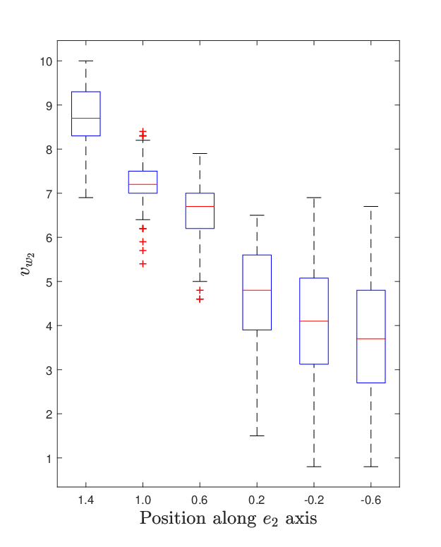
(b) Distribution of wind velocity element vw2v_{w_{2}} (m s−1\mathrm{m}\text{\,}{\mathrm{s}}^{-1} versus distances in front of the fan)
Fig. 14: Distribution of wind velocity element vw2v_{w_{2}} (m s−1\mathrm{m}\text{\,}{\mathrm{s}}^{-1} versus distances in front of the fan)

VII-A Geometric Adaptive Control for Hovering

In this section, we observe the performance of the adaptive controller for hovering flight when the quadrotor is subject to the wind.

Initially the fan is turned off, and it is turned on at about t=10t=10 seconds. The location of the quadrotor along the second inertial frame is x⁡(2)=1.0​mx(2)=1.0$\mathrm{m}$, and as such the average wind speed is about 7.3​m/s7.3$\mathrm{m}\mathrm{/}\mathrm{s}$ as shown at Figure 14.

The controller gains and parameters are chosen as

kx=16.0,kv=5.0,\displaystyle k_{x}=16.0,\quad k_{v}=5.0,
kR=1.2,kΩ=0.3,\displaystyle k_{R}=1.2,\quad k_{\Omega}=0.3,
γw1=0.3,γv1=0.3,κ1=0.0001,c1=1,\displaystyle\gamma_{w_{1}}=0.3,\quad\gamma_{v_{1}}=0.3,\quad\kappa_{1}=0.0001,\quad c_{1}=1,
γw2=0.035,γv2=0.035,κ2=0.0001,c2=1.\displaystyle\gamma_{w_{2}}=0.035,\quad\gamma_{v_{2}}=0.035,\quad\kappa_{2}=0.0001,\quad c_{2}=1.

The number of neurons in the first, hidden and output layers are

N11=6,N21=3,N31=3,\displaystyle N_{1_{1}}=6,\quad N_{2_{1}}=3,\quad N_{3_{1}}=3, (55)
N12=6,N22=3,N32=3.\displaystyle N_{1_{2}}=6,\quad N_{2_{2}}=3,\quad N_{3_{2}}=3. (56)

Experimental results are illustrated in Figure 15 and Figure 16. The trajectories without disturbance rejection are plotted in blue, and with PID controller [8] in green, and with adaptive controller in red. It can be seen that both controllers with disturbance rejection techniques improve the tracking performance. However the adaptive controller outperforms the other, while it does not result in large thrusts.

Figure 17 shows the experiment photo. The top photo is for hovering flight with the adaptive controller, and in the bottom, the quadrotor supposed to fly closer to the fan, but due to the wind it is far form the desired position22 2 For the video file this experiment, visit the FDCL YouTube channel at https://youtu.be/ouSsrDfi8DM or the experiment section of the FDCL website at http://fdcl.seas.gwu.edu/..

(a) Position error (mm)
(b) Velocity error (m s−1\mathrm{m}\text{\,}{\mathrm{s}}^{-1})

(c) Attitude error
(d) Angular velocity error (OPENr​a​ds)\frac{rad}{s}))
Fig. 15: Hovering flight (tracking errors), blue:without disturbance rejection [12], green:PID [8], red: adaptive controller

(a) Δ1\Delta_{1}, green:PID, red: adaptive with wind
(b) Δ2\Delta_{2}, green:PID, red: adaptive with wind

Refer to caption
(c) Thrust (N), blue: without disturbance rejection [12] with wind, green:PID, red: adaptive controller with wind
Fig. 16: Hovering flight (adaptive term, and thrusts), blue:without disturbance rejection [12], green:PID [8], red: adaptive controller
Refer to caption
Fig. 17: Hovering flight (snapshot), top:adaptive controller, bottom:without disturbance rejection [12].

VII-B Geometric Adaptive Control for Position Tracking

In this section, the performance of the adaptive controller for the trajectory tracking is observed. The desired trajectory is given by

xd​(t)=[−0.670.2−1.2​cos⁡(π​t12)−1.57],b1​(tk)=[100],\displaystyle x_{d}(t)=\begin{bmatrix}-0.67\\ 0.2-1.2\cos(\frac{\pi t}{12})\\ -1.57\end{bmatrix},\quad b_{1}(t_{k})=\begin{bmatrix}1\\ 0\\ 0\end{bmatrix}, (57)

which is a sinusoidal oscillation along the second inertial axis.

Figures 18–20 show the experimental data. The black lines show the desired trajectories. The trajectories without disturbance rejection are plotted in blue, and those with the proposed adaptive controller in red. It is illustrated that the proposed controller yields smaller tracking errors without excessive rotor thrust.

(a) Position (mm)
(b) Velocity (m s−1\mathrm{m}\text{\,}{\mathrm{s}}^{-1})

(c) Attitude
Fig. 18: Position tracking (position, velocity, rotation matrix) black:desired, blue:without disturbance rejection [12], red: adaptive controller

(a) Position error (mm)
(b) Velocity error (m s−1\mathrm{m}\text{\,}{\mathrm{s}}^{-1})

(c) Attitude error
(d) Angular velocity error (rad s−1\mathrm{rad}\text{\,}{\mathrm{s}}^{-1}
Fig. 19: Position tracking (tracking errors), blue:without disturbance rejection [12], red: adaptive controller

(a) Δ1\Delta_{1} for position
(b) Δ2\Delta_{2} for attitude

(c) Thrust (N\mathrm{N}), blue:without disturbance rejection [12] with wind, red: adaptive controller with wind
Fig. 20: Position tracking (adaptive terms and thrust), blue:without disturbance rejection [12], red: adaptive controller

VII-C Geometric Adaptive Control for Backflip

The illustrate the performance of the proposed control system through an agile maneuver, here we present experimental results for a backflip maneuver.

The desired trajectory is defined in the three sequences, including taking-off, backflip, and hovering. First, the quadrotor takes off to reach the desired upward velocity from t0=0​st_{0}=0$\mathrm{s}$ to t1=2.20​st_{1}=2.20$\mathrm{s}$ as follows.

xd​(t)=x0+a​t22​[001],b1d=[100],\displaystyle x_{d}(t)=x_{0}+\frac{at^{2}}{2}\begin{bmatrix}0\\ 0\\ 1\end{bmatrix},\quad b_{1_{d}}=\begin{bmatrix}1\\ 0\\ 0\end{bmatrix}, (58)

where x0=[−0.22, 0.47,−0.50]Tx_{0}=[-0.22,\,0.47,\,-0.50]^{T}, a=−0.50a=-0.50, and the quadrotor is controlled using (16)–(12).

In the next step, the attitude is controlled with (17) to rotate the quadrotor by 360∘360^{\circ} along the b1d=e1b_{1_{d}}=e_{1} axis. The desired attitude trajectory is chosen as

Rd​(t)=exp⁡(θd​(t)​b^1d),\displaystyle R_{d}(t)=\exp(\theta_{d}(t)\hat{b}_{1_{d}}), (59)

where the rotation angle is chosen as a second order polynomial of time,

θd​(t)={12​αm​(t−t1)2if t1<t<t1+δ​t212​Δt​αm​(t−t1)−12​αm​(t−t1−δ​t2)2if t1+Δt2<t<t1+68​δ​t,\theta_{d}(t)=\begin{cases}\frac{1}{2}\alpha_{m}(t-t_{1})^{2}&\text{if $t_{1}<t<t_{1}+\frac{\delta t}{2}$}\\ &\\ \frac{1}{2}\Delta_{t}\alpha_{m}(t-t_{1})&\\ -\frac{1}{2}\alpha_{m}(t-t_{1}-\frac{\delta t}{2})^{2}&\text{if $t_{1}+\frac{\Delta_{t}}{2}<t<t_{1}+\frac{6}{8}\delta t$},\end{cases} (60)

with

αm=60.0,Δt=8​παm.\displaystyle\alpha_{m}=60.0,\quad\Delta_{t}=\sqrt{\frac{8\pi}{\alpha_{m}}}. (61)

The resulting desired angular velocity is

Ωd​(t)={αm​(t−t1)​b1dif t1<t<t1+δ​t2αm​(Δt+t1−t)​b1dif t1+δ​t2<t<t1+68​δ​t,\Omega_{d}(t)=\begin{cases}\alpha_{m}(t-t_{1})b_{1_{d}}&\text{if $t_{1}<t<t_{1}+\frac{\delta t}{2}$}\\ \alpha_{m}(\Delta_{t}+t_{1}-t)b_{1_{d}}&\text{if $t_{1}+\frac{\delta t}{2}<t<t_{1}+\frac{6}{8}\delta t$},\end{cases} (62)

After backflip, again the quadrotor is controlled using (16)–(12) to make it hover at a fixed location specified as

xd​(t)=x0+a​t122​[001],b1d=[100].\displaystyle x_{d}(t)=x_{0}+\frac{at_{1}^{2}}{2}\begin{bmatrix}0\\ 0\\ 1\end{bmatrix},\quad b_{1_{d}}=\begin{bmatrix}1\\ 0\\ 0\end{bmatrix}. (63)

Figures 21–23 show the experimental results. The black lines show the desired trajectories. The trajectories without disturbance rejection are plotted in blue, and with those of the proposed adaptive controller in red. The gray lines are to separate the three stages described above. The first gray line divides the take-off from the backflip and the second one separates the backflip from the last hovering stage. For the control system presented in [12], the angular velocity diverges during the backflip stage, resulting in a large attitude tracking error afterwards. More specifically, due to wind in −e2-e_{2} direction, the quadrotor could not complete a swift rotation during the second step. Actually, it rotated only about 180∘180^{\circ} along e1e_{1} axis in the second step, and continued the rotation through the third stage, during which the quadrotor fail to regain control and crashes into the floor. See Figure 24 for snapshots.

In contrast, the proposed geometric adaptive controller with neural network result in a successful backflip maneuver followed by a stable hovering flight, as illustrated in Figure 25. It is remarkable that the neural network parameters are adjusted promptly over the short time period of the second backflip stage, to achieve the successful backflip maneuver. Such agile maneuver under the effects of wind has not been demonstrated yet33 3 For the video file of this experiment, visit the FDCL YouTube channel at https://youtu.be/a-DG2PcUu7k or the experiment section of the FDCL website at http://fdcl.seas.gwu.edu/..

(a) Position (mm)
(b) Velocity (m s−1\mathrm{m}\text{\,}{\mathrm{s}}^{-1}

(c) Attitude
Fig. 21: Backflip (position, velocity, and rotation matrix), black:desired, blue:without disturbance rejection [12], red: adaptive controller

(a) Position error (mm)
(b) Velocity error (OPENm s−1)$\mathrm{m}\text{\,}{\mathrm{s}}^{-1}$)

(c) Attitude error
(d) Angular velocity error (rad s−1\mathrm{rad}\text{\,}{\mathrm{s}}^{-1}
Fig. 22: Backflip (tracking errors), blue:without disturbance rejection [12], red: adaptive controller

(a) Δ1\Delta_{1} for position
(b) Δ2\Delta_{2} for attitude

(c) Angular velocity (rad s−1\mathrm{rad}\text{\,}{\mathrm{s}}^{-1})
(d) Thrust (N\mathrm{N})
Fig. 23: Back flip (adaptive terms, angular velocity, and thrust), black:desired, blue:without disturbance rejection [12], red: adaptive controller

Refer to caption
(a) At t=0​st=0$\mathrm{s}$

Refer to caption
(b) At t=2.20​st=2.20$\mathrm{s}$

Refer to caption
(c) At t=2.52​st=2.52$\mathrm{s}$

Refer to caption
(d) At t=2.71​st=2.71$\mathrm{s}$

Refer to caption
(e) At t=2.80​st=2.80$\mathrm{s}$

Refer to caption
(f) At t=3.24​st=3.24$\mathrm{s}$
Fig. 24: Backflip without disturbance rejection [12] (snapshots

Refer to caption
(a) At t=0​st=0$\mathrm{s}$

Refer to caption
(b) At t=2.02​st=2.02$\mathrm{s}$

Refer to caption
(c) At t=2.48​st=2.48$\mathrm{s}$

Refer to caption
(d) At t=2.55​st=2.55$\mathrm{s}$

Refer to caption
(e) At t=2.60​st=2.60$\mathrm{s}$

Refer to caption
(f) At t=2.74​st=2.74$\mathrm{s}$
Fig. 25: Backflip with the adaptive controller (snapshots)

Here we present the proof of Proposition III.1. First, in Section -D, selected identities that are used throughout the proof are presented. Then in Section -E, we analyze the error dynamics for the position tracking command, which will be integrated with the attitude error dynamics presented in -F. Finally, in Section -G, we consider the stability of the complete dynamics.

-D Identities

For any 𝒜∈ℝ3×3,x,y∈ℝ3\mathcal{A}\in\mathbb{R}^{3\times 3},x,y\in\mathbb{R}^{3}, c1,c2,c3∈ℝc_{1},c_{2},c_{3}\in\mathbb{R},

tr⁡[y​xT]=xT​y,\displaystyle\mathrm{tr}\negthickspace\left[yx^{T}\right]=x^{T}y, (64)
‖x+y‖≤‖x‖+‖y‖,\displaystyle||x+y||\leq||x||+||y||, (65)
−c1​x2+c2​x=−c12​x2−c12​[x−c2c1]2+c222​c1\displaystyle-c_{1}x^{2}+c_{2}x=-\frac{c_{1}}{2}x^{2}-\frac{c_{1}}{2}[x-\frac{c_{2}}{c_{1}}]^{2}+\frac{c_{2}^{2}}{2c_{1}}
≤−c12​x2+c222​c1,\displaystyle\leq-\frac{c_{1}}{2}x^{2}+\frac{c_{2}^{2}}{2c_{1}}, (66)
−c1​x2−c2​x​y−c3​y2≤−c1​x2+c2​x​y−c3​y2.\displaystyle-c_{1}x^{2}-c_{2}xy-c_{3}y^{2}\leq-c_{1}x^{2}+c_{2}xy-c_{3}y^{2}. (67)
𝒜T​x^+x^​𝒜=([tr⁡[𝒜]​I3×3−𝒜]​x)∧.\displaystyle\mathcal{A}^{T}\hat{x}+\hat{x}\mathcal{A}=([\mathrm{tr}\negthickspace\left[\mathcal{A}\right]I_{3\times 3}-\mathcal{A}]x)^{\wedge}. (68)

Let 𝒱0i\mathcal{V}_{0_{i}} be the part of the Lyapunov function dependent of W~i,V~i\tilde{W}_{i},\tilde{V}_{i} defined as

𝒱0i=12​γwi​tr​[W~iT​W~i]+12​γvi​tr​[V~iT​V~i],.\displaystyle\mathcal{V}_{0_{i}}=\frac{1}{2\gamma_{w_{i}}}\mathrm{tr}\negthickspace\left[\tilde{W}_{i}^{T}\tilde{W}_{i}\right]+\frac{1}{2\gamma_{v_{i}}}\mathrm{tr}\negthickspace\left[\tilde{V}_{i}^{T}\tilde{V}_{i}\right],. (69)

We find the upper bound of the following expression, defined as ℬi∈ℝ\mathcal{B}_{i}\in\mathbb{R},

ℬi=−aiT​(Δ~i)+𝒱˙0i.\displaystyle\mathcal{B}_{i}=-a_{i}^{T}(\tilde{\Delta}_{i})+\dot{\mathcal{V}}_{0_{i}}. (70)

The error dynamics of the neural network weights from (28) are give by

W~˙i=−W¯˙i,V~˙i=−V¯˙i.\displaystyle\dot{\tilde{W}}_{i}=-\dot{\bar{W}}_{i},\quad\dot{\tilde{V}}_{i}=-\dot{\bar{V}}_{i}. (71)

We substitute (25)–(26) into (71). Using (29), ℬi\mathcal{B}_{i} is rewritten as

ℬi\displaystyle\mathcal{B}_{i} =aiT​{−W~iT​[σ⁡(zi)−σ′​(zi)​zi]−W¯iT​σ′​(zi)​z~i+wi}\displaystyle=a_{i}^{T}\{-\tilde{W}_{i}^{T}[\sigma(z_{i})-\sigma^{\prime}(z_{i})z_{i}]-\bar{W}_{i}^{T}\sigma^{\prime}(z_{i})\tilde{z}_{i}+w_{i}\}
+tr⁡[W~iT​[σ⁡(zi)​aiT−σ′​(zi)​zi​aiT+κi​W¯i]]\displaystyle\quad+\mathrm{tr}\negthickspace\left[\tilde{W}_{i}^{T}[\sigma(z_{i})a_{i}^{T}-\sigma^{\prime}(z_{i})z_{i}a_{i}^{T}+\kappa_{i}\bar{W}_{i}]\right]
+tr⁡[V~iT​{xn​ni​[σ′​(zi)T​W¯i​ai]T+κi​V¯i}].\displaystyle\quad+\mathrm{tr}\negthickspace\left[\tilde{V}_{i}^{T}\{x_{nn_{i}}[\sigma^{\prime}(z_{i})^{T}\bar{W}_{i}a_{i}]^{T}+\kappa_{i}\bar{V}_{i}\}\right]. (72)

Applying (64), it reduces to

ℬi=κi​tr​[Z~iT​Z¯i]+aiT​(wi).\displaystyle\mathcal{B}_{i}=\kappa_{i}\mathrm{tr}\negthickspace\left[\tilde{Z}_{i}^{T}\bar{Z}_{i}\right]+a_{i}^{T}(w_{i}). (73)

We have

tr⁡[Z~iT​Z¯i]=tr⁡[Z~iT​Zi]−tr⁡[Z~iT​Z~i]≤||Z~i||ZMi−‖Z~i‖2.\displaystyle\mathrm{tr}\negthickspace\left[\tilde{Z}_{i}^{T}\bar{Z}_{i}\right]=\mathrm{tr}\negthickspace\left[\tilde{Z}_{i}^{T}Z_{i}\right]-\mathrm{tr}\negthickspace\left[\tilde{Z}_{i}^{T}\tilde{Z}_{i}\right]\leq||\tilde{Z}_{i}||Z_{M_{i}}-||\tilde{Z}_{i}||^{2}. (74)

The inequality (66) implies

−‖Z~i‖2+ZMi​‖Z~i‖≤−12​‖Z~i‖2+ZMi22.\displaystyle-||\tilde{Z}_{i}||^{2}+Z_{M_{i}}||\tilde{Z}_{i}||\leq-\frac{1}{2}||\tilde{Z}_{i}||^{2}+\frac{Z_{M_{i}}^{2}}{2}. (75)

Since ‖σ‖≤1,‖σ′‖≤0.25\left\|\sigma\right\|\leq 1,\,\left\|\sigma^{\prime}\right\|\leq 0.25, it can be shown that the upper bound for (31) is

‖𝒪i‖≤2+0.25​‖V~i‖​‖xn​ni‖.\displaystyle\left\|\mathcal{O}_{i}\right\|\leq 2+0.25\left\|\tilde{V}_{i}\right\|\left\|x_{nn_{i}}\right\|. (76)

From (21), the upper bound of (30) is

‖wi‖≤\displaystyle\left\|w_{i}\right\|\leq 0.25​VMi​‖W~i‖​‖xn​ni‖+WMi​‖𝒪i‖+ϵi.\displaystyle 0.25V_{M_{i}}\left\|\tilde{W}_{i}\right\|\left\|x_{nn_{i}}\right\|+W_{M_{i}}\left\|\mathcal{O}_{i}\right\|+\epsilon_{i}. (77)

Since ‖xn​ni‖≤1+‖x1i‖+‖x2i‖\left\|x_{nn_{i}}\right\|\leq 1+\left\|x_{1_{i}}\right\|+\left\|x_{2_{i}}\right\|, ‖Z~i‖≥‖W~i‖,‖Z~i‖≥‖V~i‖\left\|\tilde{Z}_{i}\right\|\geq\left\|\tilde{W}_{i}\right\|,\,\left\|\tilde{Z}_{i}\right\|\geq\left\|\tilde{V}_{i}\right\|, (21), we obtain

‖wi‖≤C1i+C2i​‖Z~i‖​(1+‖x1i‖+‖x2i‖),\displaystyle\left\|w_{i}\right\|\leq C_{1_{i}}+C_{2_{i}}||\tilde{Z}_{i}||(1+\left\|x_{1_{i}}\right\|+\left\|x_{2_{i}}\right\|), (78)

where C2i≥0.25​(VMi+WMi),C1i≥2​WMi+ϵiC_{2_{i}}\geq 0.25(V_{M_{i}}+W_{M_{i}}),\,C_{1_{i}}\geq 2W_{M_{i}}+\epsilon_{i}.

Substituting (75) and (77) into (73),

ℬi≤\displaystyle\mathcal{B}_{i}\leq −κi2​‖Z~i‖2+κi​ZMi22\displaystyle-\frac{\kappa_{i}}{2}||\tilde{Z}_{i}||^{2}+\frac{\kappa_{i}Z_{M_{i}}^{2}}{2}
+‖ai‖​{C1i+C2i​‖Z~i‖​(1+‖x1i‖+‖x2i‖)}.\displaystyle+\left\|a_{i}\right\|\{C_{1_{i}}+C_{2_{i}}||\tilde{Z}_{i}||(1+\left\|x_{1_{i}}\right\|+\left\|x_{2_{i}}\right\|)\}. (79)

-E Position Error Dynamics

Taking the derivative of (11) and substituting (8) and (2), the error dynamics are defined as

e˙x=ev,\displaystyle\dot{e}_{x}=e_{v}, (80)
m​ev˙=m​g​e3−Δ1−f​R​e3−m​x¨d.\displaystyle m\dot{e_{v}}=mge_{3}-\Delta_{1}-fRe_{3}-m\ddot{x}_{d}. (81)

Define 𝒳∈ℝ3\mathcal{X}\in\mathbb{R}^{3} as

𝒳≡fe3T​RcT​R​e3​[(e3T​RcT​R​e3)​R​e3−Rc​e3],\displaystyle\mathcal{X}\equiv\frac{f}{e_{3}^{T}R_{c}^{T}Re_{3}}[(e_{3}^{T}R_{c}^{T}Re_{3})Re_{3}-R_{c}e_{3}], (82)

where e3T​RcT​R​e3>0e_{3}^{T}R_{c}^{T}Re_{3}>0 [12]. Equation (81) is rewritten as

m​e˙v=m​g​e3−Δ1−m​x¨d−fe3T​RcT​R​e3​Rc​e3−𝒳.\displaystyle m\dot{e}_{v}=mge_{3}-\Delta_{1}-m\ddot{x}_{d}-\frac{f}{e_{3}^{T}R_{c}^{T}Re_{3}}R_{c}e_{3}-\mathcal{X}. (83)

Since b3​c=Rc​e3=−A‖A‖b_{3c}=R_{c}e_{3}=\frac{-A}{\left\|A\right\|}, f=−AT​R​e3f=-A^{T}Re_{3}, we can conclude that f=(‖A‖​Rc​e3)T​R​e3f=(\left\|A\right\|R_{c}e_{3})^{T}Re_{3}, therefore

−fe3T​RcT​R​e3​Rc​e3=A.\displaystyle-\frac{f}{e_{3}^{T}R_{c}^{T}Re_{3}}R_{c}e_{3}=A. (84)

Substituting (84), (12) into (83), the velocity error dynamics is written as

m​e˙v=−kx​ex−kv​ev−Δ~1−𝒳.\displaystyle m\dot{e}_{v}=-k_{x}e_{x}-k_{v}e_{v}-\tilde{\Delta}_{1}-\mathcal{X}. (85)

Next, we find the upper bound of 𝒳\mathcal{X}. From (84), ‖A‖=‖−fe3T​RcT​R​e3​Rc​e3‖\left\|A\right\|=\left\|-\frac{f}{e_{3}^{T}R_{c}^{T}Re_{3}}R_{c}e_{3}\right\|. Since Rc​e3R_{c}e_{3} is a unit vector, ‖A‖=‖−fe3T​RcT​R​e3‖\left\|A\right\|=\left\|-\frac{f}{e_{3}^{T}R_{c}^{T}Re_{3}}\right\|. Consequently, the norm of 𝒳\mathcal{X} can be written as

‖𝒳‖=‖A‖‖[(e3TRcTRe3)Re3−Rce3‖.\displaystyle\left\|\mathcal{X}\right\|=\left\|A\right\|\left\|[(e_{3}^{T}R_{c}^{T}Re_{3})Re_{3}-R_{c}e_{3}\right\|. (86)

Also, it is shown that ‖[(e3TRcTRe3)Re3−Rce3‖≤‖eR‖≤β<1\left\|[(e_{3}^{T}R_{c}^{T}Re_{3})Re_{3}-R_{c}e_{3}\right\|\leq\left\|e_{R}\right\|\leq\beta<1, where β=ψ1​(2−ψ1)\beta=\sqrt{\psi_{1}(2-\psi_{1})} [12]. Substituting (12) and (19), the upper bound of ‖𝒳‖\left\|\mathcal{X}\right\| is given by

‖𝒳‖≤(kx​‖ex‖+kv​‖ev‖+B1)​‖eR‖.\displaystyle\left\|\mathcal{X}\right\|\leq(k_{x}\left\|e_{x}\right\|+k_{v}\left\|e_{v}\right\|+B_{1})\left\|e_{R}\right\|. (87)

For a non-negative constant c1c_{1}, the Lyapunov function for the position dynamics is chosen as

𝒱1=12​kx​exT​ex+12​m​evT​ev+m​c1​exT​ev+𝒱01,\displaystyle\mathcal{V}_{1}=\frac{1}{2}k_{x}e_{x}^{T}e_{x}+\frac{1}{2}me_{v}^{T}e_{v}+mc_{1}e_{x}^{T}e_{v}+\mathcal{V}_{0_{1}}, (88)

where 𝒱01\mathcal{V}_{0_{1}} is given by (69). It is straightforward to show

λm​(ℳ11)​‖𝒵11‖2+𝒱01≤𝒱1≤λM​(ℳ12)​‖𝒵11‖2+𝒱01,\displaystyle\lambda_{m}(\mathcal{M}_{11})||\mathcal{Z}_{11}||^{2}+\mathcal{V}_{0_{1}}\leq\mathcal{V}_{1}\leq\lambda_{M}(\mathcal{M}_{12})||\mathcal{Z}_{11}||^{2}+\mathcal{V}_{0_{1}}, (89)

where

ℳ11=12​[kx−m​c1−m​c1m],ℳ12=12​[kxm​c1m​c1m],\displaystyle\mathcal{M}_{11}=\frac{1}{2}\begin{bmatrix}k_{x}&-mc_{1}\\ -mc_{1}&m\end{bmatrix},\quad\mathcal{M}_{12}=\frac{1}{2}\begin{bmatrix}k_{x}&mc_{1}\\ mc_{1}&m\end{bmatrix}, (90)
𝒵11=[‖ex‖,‖ev‖]T.\displaystyle\mathcal{Z}_{11}=[||e_{x}||,||e_{v}||]^{T}. (91)

If c1c_{1} is sufficiently small such that

c1<kxm,\displaystyle c_{1}<\sqrt{\frac{k_{x}}{m}}, (92)

then ℳ11,ℳ12\mathcal{M}_{11},\mathcal{M}_{12} are positive-definite.

Taking the derivative of the Lyapunov function,

𝒱˙1=\displaystyle\dot{\mathcal{V}}_{1}= kx​evT​ex+(ev+c1​ex)T​m​e˙v+m​c1​evT​ev+𝒱˙01.\displaystyle k_{x}e_{v}^{T}e_{x}+(e_{v}+c_{1}e_{x})^{T}m\dot{e}_{v}+mc_{1}e_{v}^{T}e_{v}+\dot{\mathcal{V}}_{0_{1}}. (93)

Substituting (85) into (93) and rearranging,

𝒱˙1=\displaystyle\dot{\mathcal{V}}_{1}= (m​c1−kv)​evT​ev−c1​kx​exT​ex−c1​kv​exT​ev\displaystyle(mc_{1}-k_{v})e_{v}^{T}e_{v}-c_{1}k_{x}e_{x}^{T}e_{x}-c_{1}k_{v}e_{x}^{T}e_{v}
−(ev+c1​ex)T​𝒳−(ev+c1​ex)T​Δ~1+𝒱˙01.\displaystyle-(e_{v}+c_{1}e_{x})^{T}\mathcal{X}-(e_{v}+c_{1}e_{x})^{T}\tilde{\Delta}_{1}+\dot{\mathcal{V}}_{0_{1}}. (94)

From (27), the last two terms of the above expression are the same as (70). Substituting its equivalent expression given by (79), and substituting (87),

𝒱˙1≤\displaystyle\dot{\mathcal{V}}_{1}\leq −(kv​(1−β)−m​c1)​evT​ev−c1​kx​(1−β)​exT​ex\displaystyle-(k_{v}(1-\beta)-mc_{1})e_{v}^{T}e_{v}-c_{1}k_{x}(1-\beta)e_{x}^{T}e_{x}
+c1​kv​(1+β)​‖ex‖​‖ev‖−κ12​‖Z~1‖2+κ1​ZM122\displaystyle+c_{1}k_{v}(1+\beta)\left\|e_{x}\right\|\left\|e_{v}\right\|-\frac{\kappa_{1}}{2}||\tilde{Z}_{1}||^{2}+\frac{\kappa_{1}Z_{M_{1}}^{2}}{2}
+‖a1‖​{C11+C21​‖Z~1‖​(1+‖x11‖+‖x21‖)}\displaystyle+\left\|a_{1}\right\|\{C_{1_{1}}+C_{2_{1}}||\tilde{Z}_{1}||(1+\left\|x_{1_{1}}\right\|+\left\|x_{2_{1}}\right\|)\}
+‖eR‖​{B1​(c1​‖ex‖+‖ev‖)+kx​exm​a​x​‖ev‖},\displaystyle+\left\|e_{R}\right\|\{B_{1}(c_{1}\left\|e_{x}\right\|+\left\|e_{v}\right\|)+k_{x}e_{x_{max}}\left\|e_{v}\right\|\}, (95)

where ‖ex‖≤exmax\left\|e_{x}\right\|\leq e_{x_{\max}} is used for simplifying multiplication of the three vectors, ‖eR‖​‖ex‖​‖ev‖\left\|e_{R}\right\|\left\|e_{x}\right\|\left\|e_{v}\right\|, for a fixed positive constant exmaxe_{x_{\max}}.

It is assumed that the desired trajectory is bounded such that ‖xd‖≤xdm​a​x,‖x˙d‖≤vdm​a​x\left\|x_{d}\right\|\leq x_{d_{max}},\,\left\|\dot{x}_{d}\right\|\leq v_{d_{max}}, where xdm​a​x,vdm​a​x>0x_{d_{max}},\,v_{d_{max}}>0. From (11) and x11=xx_{1_{1}}=x, x21=vx_{2_{1}}=v, ‖x1‖≤‖ex‖+xdm​a​x\left\|x_{1}\right\|\leq\left\|e_{x}\right\|+x_{d_{max}}, ‖x2‖≤‖ev‖+vdm​a​x\left\|x_{2}\right\|\leq\left\|e_{v}\right\|+v_{d_{max}}. Substituting these into (95), expanding a1a_{1}, and using (65), we obtain

𝒱˙1≤\displaystyle\dot{\mathcal{V}}_{1}\leq −(kv​(1−β)−m​c1)​evT​ev−c1​kx​(1−β)​exT​ex\displaystyle-(k_{v}(1-\beta)-mc_{1})e_{v}^{T}e_{v}-c_{1}k_{x}(1-\beta)e_{x}^{T}e_{x}
+c1​kv​(1+β)​‖ex‖​‖ev‖−κ12​‖Z~1‖2+κ1​ZM122\displaystyle+c_{1}k_{v}(1+\beta)\left\|e_{x}\right\|\left\|e_{v}\right\|-\frac{\kappa_{1}}{2}||\tilde{Z}_{1}||^{2}+\frac{\kappa_{1}Z_{M_{1}}^{2}}{2}
+C11​‖ev‖+C31​‖ev‖2+C41​‖ev‖​‖Z~1‖\displaystyle+C_{1_{1}}\left\|e_{v}\right\|+C_{3_{1}}\left\|e_{v}\right\|^{2}+C_{4_{1}}\left\|e_{v}\right\|\left\|\tilde{Z}_{1}\right\|
+c1​(C11​‖ex‖+C31​‖ex‖2+C41​‖ex‖​‖Z~1‖)\displaystyle+c_{1}(C_{1_{1}}\left\|e_{x}\right\|+C_{3_{1}}\left\|e_{x}\right\|^{2}+C_{4_{1}}\left\|e_{x}\right\|\left\|\tilde{Z}_{1}\right\|)
+(1+c1)​C31​‖ex‖​‖ev‖\displaystyle+(1+c_{1})C_{3_{1}}\left\|e_{x}\right\|\left\|e_{v}\right\|
+‖eR‖​{B1​(c1​‖ex‖+‖ev‖)+kx​exm​a​x​‖ev‖},\displaystyle+\left\|e_{R}\right\|\{B_{1}(c_{1}\left\|e_{x}\right\|+\left\|e_{v}\right\|)+k_{x}e_{x_{max}}\left\|e_{v}\right\|\}, (96)

where C11≥2​WM1+ϵ,C21≥0.25​(VM1+WM1),C31≥C21​ZM1,C41≥C21​(1+xdm​a​x+vdm​a​x)C_{1_{1}}\geq 2W_{M_{1}}+\epsilon,\,C_{2_{1}}\geq 0.25(V_{M_{1}}+W_{M_{1}}),\,C_{3_{1}}\geq C_{2_{1}}Z_{M_{1}},\,C_{4_{1}}\geq C_{2_{1}}(1+x_{d_{max}}+v_{d_{max}}).

Using (66), and defining kvβ≡kv​(1−β)−m​c1−C31k_{v_{\beta}}\equiv k_{v}(1-\beta)-mc_{1}-C_{3_{1}} and kxβ≡kx​(1−β)−C31k_{x_{\beta}}\equiv k_{x}(1-\beta)-C_{3_{1}}, the following expressions are rearranged as

−\displaystyle- kxβ​exT​ex+C11​ex≤−kxβ2​exT​ex+C1122​kxβ,\displaystyle k_{x_{\beta}}e_{x}^{T}e_{x}+C_{1_{1}}e_{x}\leq-\frac{k_{x_{\beta}}}{2}e_{x}^{T}e_{x}+\frac{C_{1_{1}}^{2}}{2k_{x_{\beta}}}, (97)
−\displaystyle- kvβ​evT​ev+C11​ev≤−kvβ2​evT​ev+C1122​kvβ.\displaystyle k_{v_{\beta}}e_{v}^{T}e_{v}+C_{1_{1}}e_{v}\leq-\frac{k_{v_{\beta}}}{2}e_{v}^{T}e_{v}+\frac{C_{1_{1}}^{2}}{2k_{v_{\beta}}}. (98)

Substituting (97)–(98) into (96) results in

𝒱˙1≤\displaystyle\dot{\mathcal{V}}_{1}\leq −c1​kxβ2​exT​ex−kvβ2​evT​ev−κ12​‖Z~1‖2+kx​v​‖ex‖​‖ev‖\displaystyle-\frac{c_{1}k_{x_{\beta}}}{2}e_{x}^{T}e_{x}-\frac{k_{v_{\beta}}}{2}e_{v}^{T}e_{v}-\frac{\kappa_{1}}{2}||\tilde{Z}_{1}||^{2}+k_{xv}\left\|e_{x}\right\|\left\|e_{v}\right\|
+C41​‖ev‖​‖Z~1‖+c1​C41​‖ex‖||Z~1||+C51\displaystyle+C_{4_{1}}||e_{v}||||\tilde{Z}_{1}||+c_{1}C_{4_{1}}||e_{x}||||\tilde{Z}_{1}||+C_{5_{1}}
+‖eR‖​{c1​B1​‖ex‖+(B1+kx​exm​a​x)​‖ev‖},\displaystyle+\left\|e_{R}\right\|\{c_{1}B_{1}\left\|e_{x}\right\|+(B_{1}+k_{x}e_{x_{max}})\left\|e_{v}\right\|\}, (99)

where kx​v=c1​[(1+β)​kv+C31]+C31k_{xv}=c_{1}[(1+\beta)k_{v}+C_{3_{1}}]+C_{3_{1}}, C51=c1​C1122​kxβ+C1122​kvβ+κ1​ZM122C_{5_{1}}=\frac{c_{1}C_{1_{1}}^{2}}{2k_{x_{\beta}}}+\frac{C_{1_{1}}^{2}}{2k_{v_{\beta}}}+\frac{\kappa_{1}Z_{M_{1}}^{2}}{2}.

-F Attitude Error Dynamics

Here, we analyze the error dynamics for the attitude tracking command. Let the attitude error function be

Ψ⁡(R,Rc)=12​tr​[I3×3−RcT​R].\displaystyle\Psi(R,R_{c})=\frac{1}{2}\mathrm{tr}\negthickspace\left[I_{3\times 3}-R_{c}^{T}R\right]. (100)

Taking the derivative of (18) and (100), and using (68), (9), and (17), the attitude error dynamics are given by

e˙R=12​(tr⁡[RT​Rc]​I3×3−RT​Rc)​eΩ≡C⁡(RcT​R)​eΩ,\displaystyle\dot{e}_{R}=\frac{1}{2}(\mathrm{tr}\negthickspace\left[R^{T}R_{c}\right]I_{3\times 3}-R^{T}R_{c})e_{\Omega}\equiv C(R_{c}^{T}R)e_{\Omega}, (101)
J​eΩ˙=−kR​eR−kΩ​eΩ−Δ~2,\displaystyle J\dot{e_{\Omega}}=-k_{R}e_{R}-k_{\Omega}e_{\Omega}-\tilde{\Delta}_{2}, (102)
Ψ˙​(R,Rc)=eRT​eΩ,\displaystyle\dot{\Psi}(R,R_{c})=e_{R}^{T}e_{\Omega}, (103)
‖C⁡(RcT​R)‖≤1.\displaystyle||C(R_{c}^{T}R)||\leq 1. (104)

For more details about proof of (101) and (103)–(104), see [12].

For a non-negative constant c2c_{2}, the Lyapunov function for the attitude dynamics is defined as

𝒱2=12​eΩT​J​eΩ+kR​Ψ​(R,Rc)+c2​eRT​J​eΩ+𝒱02,\displaystyle\mathcal{V}_{2}=\frac{1}{2}e_{\Omega}^{T}Je_{\Omega}+k_{R}\Psi(R,R_{c})+c_{2}e_{R}^{T}Je_{\Omega}+\mathcal{V}_{0_{2}}, (105)

where 𝒱02\mathcal{V}_{0_{2}} is given by (69), and

12​‖eR‖2≤Ψ⁡(R,Rc)≤12−ψ1​‖eR‖2,\displaystyle\frac{1}{2}\left\|e_{R}\right\|^{2}\leq\Psi(R,R_{c})\leq\frac{1}{2-\psi_{1}}\left\|e_{R}\right\|^{2}, (106)

with ψ1=1kR​[12​eΩ​(0)T​J​eΩ​(0)+kR​Ψ​(R⁡(0),Rc​(0))]\psi_{1}=\frac{1}{k_{R}}[\frac{1}{2}e_{\Omega}(0)^{T}Je_{\Omega}(0)+k_{R}\Psi(R(0),R_{c}(0))]. The bounds of 𝒱2\mathcal{V}_{2} are

λm​(ℳ21)​‖𝒵21‖2+𝒱02≤𝒱2≤λM​(ℳ22)​‖𝒵21‖2+𝒱02,\displaystyle\lambda_{m}(\mathcal{M}_{21})||\mathcal{Z}_{21}||^{2}+\mathcal{V}_{0_{2}}\leq\mathcal{V}_{2}\leq\lambda_{M}(\mathcal{M}_{22})||\mathcal{Z}_{21}||^{2}+\mathcal{V}_{0_{2}}, (107)

where

ℳ21=12​[kR−c2​λMJ−c2​λMJλmJ],ℳ22=12​[2​kR2−ψ1c2​λMJc2​λMJλMJ],\displaystyle\mathcal{M}_{21}=\frac{1}{2}\begin{bmatrix}k_{R}&-c_{2}\lambda_{M_{J}}\\ -c_{2}\lambda_{M_{J}}&\lambda_{m_{J}}\end{bmatrix},\mathcal{M}_{22}=\frac{1}{2}\begin{bmatrix}\frac{2k_{R}}{2-\psi_{1}}&c_{2}\lambda_{M_{J}}\\ c_{2}\lambda_{M_{J}}&\lambda_{M_{J}}\end{bmatrix}, (108)
𝒵21=[‖eR‖,‖eΩ‖]T,\displaystyle\mathcal{Z}_{21}=[||e_{R}||,||e_{\Omega}||]^{T}, (109)

with λmJ=λm​(J),λMJ=λM​(J)\lambda_{m_{J}}=\lambda_{m}(J),\lambda_{M_{J}}=\lambda_{M}(J). Provided that c2c_{2} is sufficiently small to satisfy the following inequality, the matrices ℳ21,ℳ22\mathcal{M}_{21},\mathcal{M}_{22} are positive-definite,

c2<min⁡{kR​λmJλMJ,2​kRλM​(2−ψ1)},\displaystyle c_{2}<\min\{\frac{\sqrt{k_{R}\lambda_{m_{J}}}}{\lambda_{M_{J}}},\sqrt{\frac{2k_{R}}{\lambda_{M}(2-\psi_{1})}}\}, (110)

where ψ1<2\psi_{1}<2.

The time-derivative of the Lyapunov function is given by

𝒱˙2=\displaystyle\dot{\mathcal{V}}_{2}= (eΩ+c2​eR)T​J​e˙Ω+kR​Ψ˙​(R,Rc)+c2​e˙RT​J​eΩ\displaystyle(e_{\Omega}+c_{2}e_{R})^{T}J\dot{e}_{\Omega}+k_{R}\dot{\Psi}(R,R_{c})+c_{2}\dot{e}_{R}^{T}Je_{\Omega}
+𝒱˙02.\displaystyle+\dot{\mathcal{V}}_{0_{2}}. (111)

Substituting error dynamics (101)–(104), (4), and (17),

𝒱˙2\displaystyle\dot{\mathcal{V}}_{2} =(eΩ+c2​eR)T​(−kR​eR−kΩ​eΩ−Δ~2)\displaystyle=(e_{\Omega}+c_{2}e_{R})^{T}(-k_{R}e_{R}-k_{\Omega}e_{\Omega}-\tilde{\Delta}_{2})
+kR​eRT​eΩ+c2​C​(RcT​R)​eΩT​J​eΩ+𝒱˙02.\displaystyle\quad+k_{R}e_{R}^{T}e_{\Omega}+c_{2}C(R_{c}^{T}R)e_{\Omega}^{T}Je_{\Omega}+\dot{\mathcal{V}}_{0_{2}}. (112)

From (67), (104), and ‖J‖≤λMJ\left\|J\right\|\leq\lambda_{M_{J}},

𝒱˙2≤\displaystyle\dot{\mathcal{V}}_{2}\leq −c2​kR​eRT​eR+c2​kΩ​‖eR‖​‖eΩ‖−(kΩ−c2​λMJ)​eΩT​eΩ\displaystyle-c_{2}k_{R}e_{R}^{T}e_{R}+c_{2}k_{\Omega}||e_{R}||||e_{\Omega}||-(k_{\Omega}-c_{2}\lambda_{M_{J}})e_{\Omega}^{T}e_{\Omega}
−(eΩ+c2​eR)T​(Δ~2)+𝒱˙02.\displaystyle-(e_{\Omega}+c_{2}e_{R})^{T}(\tilde{\Delta}_{2})+\dot{\mathcal{V}}_{0_{2}}. (113)

From (27), the last two terms of this expression are identical to (70). Substituting its equivalent expression given by (79),

𝒱˙2≤\displaystyle\dot{\mathcal{V}}_{2}\leq −c2​kR​eRT​eR+c2​kΩ​‖eR‖​‖eΩ‖−(kΩ−c2​λMJ)​eΩT​eΩ\displaystyle-c_{2}k_{R}e_{R}^{T}e_{R}+c_{2}k_{\Omega}||e_{R}||||e_{\Omega}||-(k_{\Omega}-c_{2}\lambda_{M_{J}})e_{\Omega}^{T}e_{\Omega}
−κ22​‖Z~2‖2+κ2​ZM222\displaystyle-\frac{\kappa_{2}}{2}||\tilde{Z}_{2}||^{2}+\frac{\kappa_{2}Z_{M_{2}}^{2}}{2}
+‖a2‖​{C12+C22​‖Z~2‖​(1+‖E⁡(R)‖+‖Ω‖)}.\displaystyle+\left\|a_{2}\right\|\{C_{1_{2}}+C_{2_{2}}||\tilde{Z}_{2}||(1+\left\|E(R)\right\|+\left\|\Omega\right\|)\}. (114)

It is assumed that ‖Δ¯˙1‖≤δ2\left\|\dot{\bar{\Delta}}_{1}\right\|\leq\delta_{2} and the desired trajectory is designed such that ‖x˙˙˙d‖≤δ3\left\|\dddot{x}_{d}\right\|\leq\delta_{3}, where δ2,δ3>0\delta_{2},\,\delta_{3}>0. Thus ‖m​x˙˙˙d+Δ¯˙1‖≤B2\left\|m\dddot{x}_{d}+\dot{\bar{\Delta}}_{1}\right\|\leq B_{2}. Taking the derivative of (12), it can be shown that

‖A˙‖≤kx​‖ev‖+kv​‖e˙v‖+B2.\displaystyle\left\|\dot{A}\right\|\leq k_{x}\left\|e_{v}\right\|+k_{v}\left\|\dot{e}_{v}\right\|+B_{2}. (115)

From (14), R˙c=[b˙1​c,b˙2​c,b˙3​c]\dot{R}_{c}=[\dot{b}_{1c},\dot{b}_{2c},\dot{b}_{3c}]. Let C=−b3c×b1dC=-b_{3_{c}}\times b_{1_{d}}. We have

b˙1​c=b˙2​c×b3​c+b2​c×b˙3​c,\displaystyle\dot{b}_{1c}=\dot{b}_{2c}\times b_{3c}+b_{2c}\times\dot{b}_{3c}, (116)
b˙2​c=−C˙‖C‖+C⁡(C⋅C)‖C‖3,\displaystyle\dot{b}_{2c}=-\frac{\dot{C}}{||C||}+\frac{C(C\cdot C)}{||C||^{3}}, (117)
b˙3​c=−A˙‖A‖+A⁡(A⋅A)‖A‖3.\displaystyle\dot{b}_{3c}=-\frac{\dot{A}}{||A||}+\frac{A(A\cdot A)}{||A||^{3}}. (118)

From (19), (115), and (118),

‖b˙3​c‖≤2​kx​‖ev‖+kv​‖e˙v‖+B2kx​‖ex‖+kv​‖ev‖+B1≡B3.\displaystyle\left\|\dot{b}_{3c}\right\|\leq 2\frac{k_{x}\left\|e_{v}\right\|+k_{v}\left\|\dot{e}_{v}\right\|+B_{2}}{k_{x}\left\|e_{x}\right\|+k_{v}\left\|e_{v}\right\|+B_{1}}\equiv B_{3}. (119)

It is assumed that the desired trajectory is designed such that ‖b˙1d‖≤δ4\left\|\dot{b}_{1_{d}}\right\|\leq\delta_{4}, where δ4>0\delta_{4}>0. Using (119), it can be shown that ‖C˙‖≤B3+δ4\left\|\dot{C}\right\|\leq B_{3}+\delta_{4}. From (117), as ‖C‖≤1\left\|C\right\|\leq 1,

‖b˙2​c‖≤2​(B3+δ4),\displaystyle\left\|\dot{b}_{2c}\right\|\leq 2(B_{3}+\delta_{4}), (120)

From (116), (119)–(120)

‖b˙1​c‖≤3​B3+2​δ4.\displaystyle\left\|\dot{b}_{1c}\right\|\leq 3B_{3}+2\delta_{4}. (121)

Thus, from (119)–(121), it can be shown that ‖R˙c‖≤B4\left\|\dot{R}_{c}\right\|\leq B_{4}, for a positive B4B_{4}. From (3), ‖Ωc‖≤B4\left\|\Omega_{c}\right\|\leq B_{4}. Since (18), ‖Ω‖≤‖eΩ‖+B4\left\|\Omega\right\|\leq\left\|e_{\Omega}\right\|+B_{4}.

We have ‖E⁡(R)‖≤Em​a​x\left\|E(R)\right\|\leq E_{max} for a positive Em​a​xE_{max}. Substituting these into (114), and expanding a2a_{2} with(65),

𝒱˙2≤\displaystyle\dot{\mathcal{V}}_{2}\leq −c2​kR​eRT​eR+c2​kΩ​‖eR‖​‖eΩ‖−(kΩ−c2​λMJ)​eΩT​eΩ\displaystyle-c_{2}k_{R}e_{R}^{T}e_{R}+c_{2}k_{\Omega}||e_{R}||||e_{\Omega}||-(k_{\Omega}-c_{2}\lambda_{M_{J}})e_{\Omega}^{T}e_{\Omega}
−κ22​‖Z~2‖2+κ2​ZM222\displaystyle-\frac{\kappa_{2}}{2}||\tilde{Z}_{2}||^{2}+\frac{\kappa_{2}Z_{M_{2}}^{2}}{2}
+C12​‖eΩ‖+C32​‖eΩ‖2+C42​‖eΩ‖​‖Z~2‖\displaystyle+C_{1_{2}}\left\|e_{\Omega}\right\|+C_{3_{2}}\left\|e_{\Omega}\right\|^{2}+C_{4_{2}}\left\|e_{\Omega}\right\|\left\|\tilde{Z}_{2}\right\|
+c2​(C12​‖eR‖+C42​‖eR‖​‖Z~2‖)\displaystyle+c_{2}(C_{1_{2}}\left\|e_{R}\right\|+C_{4_{2}}\left\|e_{R}\right\|\left\|\tilde{Z}_{2}\right\|)
+c2​C32​‖eR‖​‖eΩ‖,\displaystyle+c_{2}C_{3_{2}}\left\|e_{R}\right\|\left\|e_{\Omega}\right\|, (122)

where C12≥2​WM2+ϵ2,C22≥0.25​(VM2+WM2),C32≥C22​ZM2,C42≥C22​(1+Em​a​x+B4)C_{1_{2}}\geq 2W_{M_{2}}+\epsilon_{2},\,C_{2_{2}}\geq 0.25(V_{M_{2}}+W_{M_{2}}),\,C_{3_{2}}\geq C_{2_{2}}Z_{M_{2}},\,C_{4_{2}}\geq C_{2_{2}}(1+E_{max}+B_{4}). Using (66), the following expressions are rearranged into

−\displaystyle- kR​eRT​eR+C12​‖eR‖≤−kR2​eRT​eR+C1222​kR,\displaystyle k_{R}e_{R}^{T}e_{R}+C_{1_{2}}||e_{R}||\leq-\frac{k_{R}}{2}e_{R}^{T}e_{R}+\frac{C_{1_{2}}^{2}}{2k_{R}}, (123)
−\displaystyle- kΩβ​eΩT​eΩ+C12​‖eΩ‖≤−kΩβ2​eΩT​eΩ+C1222​kΩβ,\displaystyle k_{\Omega_{\beta}}e_{\Omega}^{T}e_{\Omega}+C_{1_{2}}||e_{\Omega}||\leq-\frac{k_{\Omega_{\beta}}}{2}e_{\Omega}^{T}e_{\Omega}+\frac{C_{1_{2}}^{2}}{2k_{\Omega_{\beta}}}, (124)

where kΩβ=kΩ−c2​λMJ−C32k_{\Omega_{\beta}}=k_{\Omega}-c_{2}\lambda_{M_{J}}-C_{3_{2}}. Then substituting (123)–(124) in (122)

𝒱˙2≤\displaystyle\dot{\mathcal{V}}_{2}\leq −c2​kR2​eRT​eR−kΩβ2​eΩT​eΩ−κ22​‖Z~2‖2\displaystyle-\frac{c_{2}k_{R}}{2}e_{R}^{T}e_{R}-\frac{k_{\Omega_{\beta}}}{2}e_{\Omega}^{T}e_{\Omega}-\frac{\kappa_{2}}{2}||\tilde{Z}_{2}||^{2}
+kR​Ω​‖eR‖​‖eΩ‖\displaystyle+k_{R\Omega}||e_{R}||||e_{\Omega}||
+C42​‖eΩ‖​‖Z~2‖+c2​C42​‖eR‖||Z~2||+C52.\displaystyle+C_{4_{2}}||e_{\Omega}||||\tilde{Z}_{2}||+c_{2}C_{4_{2}}||e_{R}||||\tilde{Z}_{2}||+C_{5_{2}}. (125)

where kR​Ω=c2​(κΩ+C32),C52=c2​C2122​kR+C2122​kΩβ+κ2​ZM222k_{R\Omega}=c_{2}(\kappa_{\Omega}+C_{3_{2}}),\,C_{5_{2}}=\frac{c_{2}C_{2_{1}}^{2}}{2k_{R}}+\frac{C_{2_{1}}^{2}}{2k_{\Omega_{\beta}}}+\frac{\kappa_{2}Z_{M_{2}}^{2}}{2}.

-G Stability Proof for Quadrotor Dynamics

Here, we combine the position error dynamics and the attitude error dynamics to show the stability properties of the complete controlled quadrotor. The Lyapunov function is chosen as 𝒱=𝒱1+𝒱2\mathcal{V}=\mathcal{V}_{1}+\mathcal{V}_{2}, where 𝒱1,𝒱2\mathcal{V}_{1},\mathcal{V}_{2} are given by (88), (105). From (89) and (107), the bound on 𝒱\mathcal{V} is given by

λm\displaystyle\lambda_{m} (ℳ11)​‖𝒵11‖2+λm​(ℳ21)​‖𝒵21‖2+𝒱01+𝒱02≤𝒱\displaystyle(\mathcal{M}_{11})||\mathcal{Z}_{11}||^{2}+\lambda_{m}(\mathcal{M}_{21})||\mathcal{Z}_{21}||^{2}+\mathcal{V}_{0_{1}}+\mathcal{V}_{0_{2}}\leq\mathcal{V}
≤λM​(ℳ12)​‖𝒵11‖2+λM​(ℳ22)​‖𝒵21‖2+𝒱01+𝒱02.\displaystyle\leq\lambda_{M}(\mathcal{M}_{12})||\mathcal{Z}_{11}||^{2}+\lambda_{M}(\mathcal{M}_{22})||\mathcal{Z}_{21}||^{2}+\mathcal{V}_{0_{1}}+\mathcal{V}_{0_{2}}. (126)

The upper bound can be rewritten as

𝒱≤\displaystyle\mathcal{V}\leq 12​𝒵1T​𝒩1′​𝒵1+12​𝒵2T​𝒩2′​𝒵2+12​𝒵3T​𝒩3′​𝒵3,\displaystyle\frac{1}{2}\mathcal{Z}_{1}^{T}\mathcal{N}_{1}^{\prime}\mathcal{Z}_{1}+\frac{1}{2}\mathcal{Z}_{2}^{T}\mathcal{N}_{2}^{\prime}\mathcal{Z}_{2}+\frac{1}{2}\mathcal{Z}_{3}^{T}\mathcal{N}_{3}^{\prime}\mathcal{Z}_{3}, (127)

where

𝒩1′=[kx2m​c10m​c1m20001min⁡{γw1,γv1}],\displaystyle\mathcal{N}_{1}^{\prime}=\begin{bmatrix}\frac{k_{x}}{2}&mc_{1}&0\\ mc_{1}&\frac{m}{2}&0\\ 0&0&\frac{1}{\min\{\gamma_{w_{1}},\gamma_{v_{1}}\}}\end{bmatrix},
𝒩2′=[kR2−ψ2c2​λMJ0c2​λMJλMJ0001min⁡{γw2,γv2}],\displaystyle\mathcal{N}_{2}^{\prime}=\begin{bmatrix}\frac{k_{R}}{2-\psi_{2}}&c_{2}\lambda_{M_{J}}&0\\ c_{2}\lambda_{M_{J}}&\lambda_{M_{J}}&0\\ 0&0&\frac{1}{\min\{\gamma_{w_{2}},\gamma_{v_{2}}\}}\end{bmatrix},
𝒩3′=[kx2000m200012−ψ2],\displaystyle\mathcal{N}_{3}^{\prime}=\begin{bmatrix}\frac{k_{x}}{2}&0&0\\ 0&\frac{m}{2}&0\\ 0&0&\frac{1}{2-\psi_{2}}\end{bmatrix},
𝒵1=[‖ex‖,‖ev‖,‖Z~1‖]T,𝒵2=[‖eR‖,‖eΩ‖,‖Z~2‖]T,\displaystyle\mathcal{Z}_{1}=[||e_{x}||,\left\|e_{v}\right\|,||\tilde{Z}_{1}||]^{T},\quad\mathcal{Z}_{2}=[\left\|e_{R}\right\|,||e_{\Omega}||,||\tilde{Z}_{2}||]^{T},
𝒵3=[‖ex‖,‖ev‖,‖eR‖]T.\displaystyle\mathcal{Z}_{3}=[\left\|e_{x}\right\|,||e_{v}||,||e_{R}||]^{T}.

As discussed above, the matrices 𝒩1′,𝒩2′,𝒩3′\mathcal{N}_{1}^{\prime},\mathcal{N}_{2}^{\prime},\mathcal{N}_{3}^{\prime} are positive-definite if c1,c2c_{1},c_{2} are sufficiently small.

The derivative of the Lyapunov function is 𝒱˙=𝒱˙1+𝒱˙2\dot{\mathcal{V}}=\dot{\mathcal{V}}_{1}+\dot{\mathcal{V}}_{2}. From (99) and (125), it can be written as

𝒱˙≤\displaystyle\dot{\mathcal{V}}\leq −12​𝒵1T​𝒩1​𝒵1−12​𝒵2T​𝒩2​𝒵2−12​𝒵3T​𝒩3​𝒵3+C5,\displaystyle-\frac{1}{2}\mathcal{Z}_{1}^{T}\mathcal{N}_{1}\mathcal{Z}_{1}-\frac{1}{2}\mathcal{Z}_{2}^{T}\mathcal{N}_{2}\mathcal{Z}_{2}-\frac{1}{2}\mathcal{Z}_{3}^{T}\mathcal{N}_{3}\mathcal{Z}_{3}+C_{5}, (128)

where C5=C51+C52C_{5}=C_{5_{1}}+C_{5_{2}}, and

𝒩1=[c1​kxβ2−kx​v2−c1​C41−kx​v2kvβ2−C41−c1​C41−C41κ1],\displaystyle\mathcal{N}_{1}=\begin{bmatrix}\frac{c_{1}k_{x_{\beta}}}{2}&-\frac{k_{xv}}{2}&-c_{1}C_{4_{1}}\\ -\frac{k_{xv}}{2}&\frac{k_{v_{\beta}}}{2}&-C_{4_{1}}\\ -c_{1}C_{4_{1}}&-C_{4_{1}}&\kappa_{1}\end{bmatrix}, (129)
𝒩2=[c2​kR2−kR​Ω−c2​C42−kR​ΩkΩβ−C42−c2​C42−C42κ2],\displaystyle\mathcal{N}_{2}=\begin{bmatrix}\frac{c_{2}k_{R}}{2}&-k_{R\Omega}&-c_{2}C_{4_{2}}\\ -k_{R\Omega}&k_{\Omega_{\beta}}&-C_{4_{2}}\\ -c_{2}C_{4_{2}}&-C_{4_{2}}&\kappa_{2}\end{bmatrix}, (130)
𝒩3=[c1​kxβ2−kx​v2−c1​B1−kx​v2c1​kvβ2−B1−kx​exm​a​x−c1​B1−B1−kx​exm​a​xc2​kR2].\displaystyle\mathcal{N}_{3}=\begin{bmatrix}\frac{c_{1}k_{x_{\beta}}}{2}&-\frac{k_{xv}}{2}&-c_{1}B_{1}\\ -\frac{k_{xv}}{2}&\frac{c_{1}k_{v_{\beta}}}{2}&-B_{1}-k_{x}e_{x_{max}}\\ -c_{1}B_{1}&-B_{1}-k_{x}e_{x_{max}}&\frac{c_{2}k_{R}}{2}\end{bmatrix}. (131)

We can show that choosing sufficiently large kxk_{x}, kvk_{v}, kRk_{R}, kΩk_{\Omega}, γwi,γvi\gamma_{w_{i}},\gamma_{v_{i}}, κi\kappa_{i}, and sufficiently small cic_{i}, for i∈{1,2}i\in\{1,2\}, the matrices 𝒩1,𝒩2,𝒩3\mathcal{N}_{1},\,\mathcal{N}_{2},\,\mathcal{N}_{3} become positive definite. Consequently, there exists μ>0\mu>0 such that

𝒱˙≤−ν​𝒱+C5,\displaystyle\dot{\mathcal{V}}\leq-\nu\mathcal{V}+C_{5}, (132)

If 𝒱>C5ν\mathcal{V}>\frac{C_{5}}{\nu}, then 𝒱˙<0\dot{\mathcal{V}}<0. Therefore, according to [22], ex,ev,eR,eΩ,Z~1e_{x},e_{v},e_{R},e_{\Omega},\tilde{Z}_{1} and Z~2\tilde{Z}_{2} are bounded and converge exponentially to the set 𝒟\mathcal{D}

𝒟\displaystyle\mathcal{D} ={ex,ev,eR,eΩ∈ℝ3,Z~1∈ℝN11+N21+2×N21+N31,\displaystyle=\{e_{x},e_{v},e_{R},e_{\Omega}\in\mathbb{R}^{3},\tilde{Z}_{1}\in\mathbb{R}^{N_{1_{1}}+N_{2_{1}}+2\times N_{2_{1}}+N_{3_{1}}},
Z~2∈ℝN12+N22+2×N22+N32|‖ex‖2+‖ev‖2+‖eR‖2\displaystyle\tilde{Z}_{2}\in\mathbb{R}^{N_{1_{2}}+N_{2_{2}}+2\times N_{2_{2}}+N_{3_{2}}}\arrowvert\left\|e_{x}\right\|^{2}+\left\|e_{v}\right\|^{2}+\left\|e_{R}\right\|^{2}
+‖eΩ‖2+1γ1∥Z~1∥2+1γ2∥Z~2∥2≤C5ν},\displaystyle+\left\|e_{\Omega}\right\|^{2}+\frac{1}{\gamma_{1}}\|\tilde{Z}_{1}\|^{2}+\frac{1}{\gamma_{2}}\|\tilde{Z}_{2}\|^{2}\leq\frac{C_{5}}{\nu}\}, (133)

where γ1=max⁡{γv1,γw1},γ2=max⁡{γv2,γw2}\gamma_{1}=\max\{\gamma_{v_{1}},\gamma_{w_{1}}\},\,\gamma_{2}=\max\{\gamma_{v_{2}},\gamma_{w_{2}}\}.

Acknowledgment

The authors would like to especially thank Mr. Kanishke Gamagedara for his contribution to the drone hardware platform which is used for experimental validation, and its maintenance.

References

  • [1] R. Gill and R. D’Andrea, “Propeller thrust and drag in forward flight,” in 2017 IEEE Conference on Control Technology and Applications (CCTA), Aug 2017, pp. 73–79.
  • [2] W. Craig, D. Yeo, and D. A. Paley, “Dynamics of a rotor-pendulum with a small, stiff propeller in wind,” in ASME 2016 Dynamic Systems and Control Conference, vol. 1, no. DSCC2016-9774. ASME, Oct. 2016, pp. V001T05A001–10. [Online]. Available: http://dx.doi.org/10.1115/DSCC2016-9774
  • [3] M. Bisheban and T. Lee, “Computational geometric system identification for the attitude dynamics on SO(3),” International Journal of Control, Automation and Systems, vol. 15, no. 6, pp. 2776–2785, Dec 2017. [Online]. Available: https://doi.org/10.1007/s12555-016-0714-2
  • [4] ——, “Computational geometric identification for quadrotor dynamics in wind fields,” in Proceedings of the IEEE Conference on Control Technology and Applications, Kohala Coast, Hawai’i, USA, August 2017, pp. 1153–1158.
  • [5] N. K. Tran, E. Bulka, and M. Nahon, “Quadrotor control in a wind field,” in 2015 International Conference on Unmanned Aircraft Systems (ICUAS), June 2015, pp. 320–328.
  • [6] M. Bangura and R. Mahony, “Thrust control for multirotor aerial vehicles,” IEEE Transactions on Robotics, vol. 33, no. 99, pp. 1–16, April 2017.
  • [7] W. S. Craig, D. W. Yeo, and D. A. Paley, “Geometric control of a quadrotor in wind with flow sensing and thrust constraints: Attitude and position control,” in AIAA Scitech 2019 Forum, 2019, p. 1192.
  • [8] F. Goodarzi, D. Lee, and T. Lee, “Geometric nonlinear pid control of a quadrotor uav on SE(3),” in 2013 European Control Conference (ECC), July 2013, pp. 3845–3850.
  • [9] ——, “Geometric adaptive tracking control of a quadrotor unmanned aerial vehicle on SE(3),” ASME Journal of Dynamic Systems, Measurement, and Control, vol. 137, no. 9, Sep. 2015.
  • [10] D. Mellinger, N. Michael, and V. Kumar, “Trajectory generation and control for precise aggressive maneuvers with quadrotors,” The International Journal of Robotics Research, vol. 31, no. 5, pp. 664–674, 2012. [Online]. Available: https://doi.org/10.1177/0278364911434236
  • [11] C. Nicol, C. J. B. Macnab, and A. Ramirez-Serrano, “Robust neural network control of a quadrotor helicopter,” in 2008 Canadian Conference on Electrical and Computer Engineering, May 2008, pp. 001 233–001 238.
  • [12] T. Lee, M. Leok, and N. McClamroch, “Geometric tracking control of a quadrotor aerial vehicle on 𝖲𝖤⁡(𝟥)\mathsf{SE(3)},” in Proceedings of the IEEE Conference on Decision and Control, Atlanta, GA, Dec. 2010, pp. 5420–5425.
  • [13] M. Bisheban and T. Lee, “Geometric adaptive control for a quadrotor uav with wind disturbance rejection,” in 2018 IEEE Conference on Decision and Control (CDC), Dec 2018, pp. 2816–2821.
  • [14] K. Hornik, M. Stinchcombe, and H. White, “Multilayer feedforward networks are universal approximators,” Neural networks, vol. 2, no. 5, pp. 359–366, 1989.
  • [15] P. A. Ioannou and J. Sun, Robust Adaptive Control. Upper Saddle River, NJ, USA: Prentice-Hall, Inc., 1995.
  • [16] T. Lee and Y. Kim, “Nonlinear adaptive flight control using backstepping and neural networks controller,” Journal of Guidance, Control, and Dynamics, vol. 24, no. 4, pp. 675–682, 2001.
  • [17] T. Lee, M. Leok, and N. McClamroch, “Nonlinear robust tracking control of a quadrotor UAV on 𝖲𝖤⁡(𝟥)\mathsf{SE(3)},” Asian Journal of Control, vol. 15, no. 2, pp. 391–408, Mar. 2013.
  • [18] G. D. Padfield, Helicopter flight dynamics: the theory and application of flying qualities and simulation modelling. Blackwill Publishing, 2007.
  • [19] G. M. Hoffmann, H. Huang, S. L. Waslander, and C. J. Tomlin, “Precision flight control for a multi-vehicle quadrotor helicopter testbed,” Control Engineering Practice, vol. 19, no. 9, pp. 1023–1036, 2011.
  • [20] N. Sydney, B. Smyth, and D. A. Paley, “Dynamic control of autonomous quadrotor flight in an estimated wind field,” in Proceedings of the IEEE Conference on Decision and Control, December 2013, pp. 3609–3616.
  • [21] M. Bisheban, “Geometric estimation and control of quadrotor UAVs in wind fields,” Ph.D. dissertation, The George Washington University, 2018.
  • [22] H. Khalil, “Noninear systems,” Prentice-Hall, New Jersey, vol. 2, no. 5, pp. 5–1, 1996.