Learning a Lattice Planner Control Set for Autonomous Vehicles
Abstract
This paper introduces a method to compute a sparse lattice planner control set that is suited to a particular task by learning from a representative dataset of vehicle paths. To do this, we use a scoring measure similar to the Fréchet distance and propose an algorithm for evaluating a given control set according to the scoring measure. Control actions are then selected from a dense control set according to an objective function that rewards improvements in matching the dataset while also encouraging sparsity. This method is evaluated across several experiments involving real and synthetic datasets, and it is shown to generate smaller control sets when compared to the previous state-of-the-art lattice control set computation technique, with these smaller control sets maintaining a high degree of manoeuvrability in the required task. This results in a planning time speedup of up to 4.31x when using the learned control set over the state-of-the-art computed control set. In addition, we show the learned control sets are better able to capture the driving style of the dataset in terms of path curvature.
I Introduction
A crucial portion of autonomous vehicle navigation is path planning. It is important for autonomous vehicles to be able to quickly generate a collision-free, kinematically feasible path towards their goal that minimizes the total cost of the path. An algorithm commonly used in path planning is the lattice planner[1]. The lattice planner is a graph-based approach to the path planning problem that reduces the search space into a uniform discretization of vertices corresponding to positions and headings. Each vertex in the discretization is connected to other points by kinematically feasible motion primitives, known as control actions[2]. The lattice planner thus reduces the path planning problem into a graph-search problem, which can be solved with A* or any other appropriate graph search algorithm[3, 4, 5, 6]. An example of a lattice graph is shown in Figure 1.

I-A Contributions
This work focuses on the task of leveraging data gathered from a particular task to optimize a sparse set of motion primitives, known as a control set, by removing control actions that are less important for planning paths similar to those in the dataset. This sparse control set should be selected such that it is specialized with respect to a given dataset; that is, it can reproduce a dataset of paths of an autonomous vehicle generated from human operation or demonstration. The sparsity of the learned control set reduces the number of edges in the search graph, and thus allows for faster online path computation. In addition, the learned control set should capture some characteristics of the driving style present in the dataset, and the learned control set should not sacrifice path quality or manoeuvrability. To learn such a control set, we require a way to measure how closely we can match paths from the dataset using a lattice planner with the given control set, as well as a way to select a sparse subset.
In this work, the first contribution is a novel algorithm for finding the closest path in a lattice graph to a given path according to a modified version of the Fréchet distance. The second contribution is a method to select a sparse subset of a given control set that still retains the ability to execute paths in a given dataset, while also capturing the driving style present in the dataset. These algorithms are tested on both real human-driven data as well as synthetic data, and compared to the state-of-the-art lattice control set reduction technique[7].
I-B Related Work
In previous work, data-driven motion planning has often focused on learning search heuristics or policies for the motion planner rather than learning the underlying structure of the planner itself. Ichter et al. developed a method for learning a sampling distribution for RRT* motion planning[8]. Imitation learning can also be used to learn a search heuristic based on previously planned optimal paths[9, 10]. Paden et al. have developed a method for optimizing search heuristics for a given kinodynamic planning problem[11]. Xu et al. used reinforcement learning to learn a control policy for quadcopters by training on MPC outputs[12].
For work involving lattice planner control set optimization, Pivtoraiko et al. have developed a D*-like (DL) algorithm for finding a subset of a lattice control set that spans the same reachability of the original control set, but does so within a multiplicative factor of each original control action’s arc length[7]. This algorithm does not rely on data, but instead relies on the structure of the original control set to find redundancy. In contrast, our method attempts to leverage data for a particular application to optimize the control set. This paper uses the DL algorithm as the state-of-the-art comparison for the quality of the presented learning algorithm.
To optimize a planner, we require a measure of similarity between two paths. This has been discussed in the field of path clustering [13], where measures such as the pointwise Euclidean distance, Hausdorff distance[14], the Longest Common Sub-Sequence, and the Fréchet distance[15] are commonly used.
The work most closely related to the process of matching a specific path in a graph is the map-matching problem[16, 17]. The problem entails finding a path in a planar graph embedded in Euclidean space that best matches a given polygonal curve according to the Fréchet distance. However, unlike our work, their algorithm requires the full graph to be defined beforehand, and cannot be used if the graph is implicitly defined in terms of the lattice control set. Another similar problem is that of following a path in the workspace for a redundant manipulator[18, 19].
In terms of driving style, Macadam gives a broad overview of the driving task[20]. This paper focuses on the properties of paths and not trajectories. For the driving style of a given path, one of the most intuitive indicators is the vehicle’s steering function, which under the commonly used bicycle model[21], is directly related to path curvature. As such, curvature serves as a natural measure for comparing the driving styles of different paths. A path with points of high curvature corresponds to a a more aggressive steering function, and vice versa.
II Sparse Control Set Problem Formulation
II-A Lattice Planner Preliminaries
In this work, the robot navigates lattice points within a subset , discretized with and resolution and , respectively, and with heading set [3]. Navigation between lattice points in is done according to control actions present in a control set . For a given control set , each heading has an associated control subset , and the control actions in that set can be applied at any lattice point . This action results in a transition to a point where the relative position is fixed for that action. Thus, the action connects all identically arranged pairs of lattice points[22]. These connections define edges , and these lattice points define vertices in a lattice graph . An example of a lattice graph is given in Figure 1. Each control action in has a corresponding path, and the path formed by the concatenation of control actions in the lattice graph is denoted as .
II-B Problem Formulation
Our main goal is to learn a sparse control set for a lattice planner that retains the driving style that is present in a dataset. We start with a dense control set and then incrementally generate a subset by selecting the control actions that best improve the ability of the lattice planner to execute the paths present in the dataset. In essence, we would like the dataset paths to become approximate subpaths of lattice paths formed using our learned control set, as in Figure 2. While optimizing in this way, however, we also want to encourage sparsity, since larger control sets result in longer planning times. We can formally state the high-level problem.
High-Level Problem. Given a dense set of control actions , and a dataset of representative paths , compute a minimal subset that allows a lattice planner to execute the paths present in .
We split the high-level problem into two sub-problems. The first is measuring how well control sets match the dataset, and the second is optimizing the control set accordingly.
Subproblem 1. Given a path and a set of control actions , compute how well executes according to a scoring measure .
Subproblem 2. Given a scoring measure , a dataset of paths , and a dense set of control actions , select as small a subset of , , as possible that best executes in aggregate according to a scoring measure .
III Sparse Control Set Generation
III-A Scoring Measure
To find the closest path generated by a lattice planner, , to a path in the dataset, , we first need a scoring measure to evaluate the similarity of two paths. For two paths parameterized by , and two monotonic increasing onto functions , the Fréchet distance is given by
However, we would like a scoring measure that rewards for matching closely at each point along the path, where points of comparison are at equal arc lengths along each path. This means that rather than allowing any monotonic increasing traversal of the paths during distance computation as in the Fréchet distance, the paths should be traversed at the same rate. In other words, if both paths were traversed at a constant velocity, then the scoring measure should compare points that are reached at the same time. When traversing both paths at the same rate, path pairs with a low score are likely to have similar driving styles along the entire path.
We therefore modify the Fréchet distance as follows. For a given path to match with arc length , a matching path that is at least as long as , and where is an arc length parameterization of both paths, then our scoring measure, denoted as , is
| (1) |

An advantage of using this measure instead of the Fréchet distance is that its simplicity allows for faster computation than the discrete Fréchet distance in a graph[23]. Note that this scoring measure is no longer a distance metric, as it is asymmetrical. The fact that we perform a comparison only along the arc length of (and no further) is motivated as follows: rather than forcing the lattice path to be the same length as , we can plan to be arbitrarily longer and then truncate to the arc length of . This opens up a greater number of terminal lattice vertices when computing , which we have found results in closer matching paths and faster runtime. The generation of is discussed in further detail in Section III-B.
Let us now assume that we are calculating for two discrete paths, sampled with respect to arc length with segments of equal length . In Appendix -B, we include implementation details, including how to handle paths with length not integer-divisible by . Let contain sampled path points, , where the point is the origin. Let denote the path point of each respective path. Then Equation (1) simplifies to
| (2) |
Equation (2) can be evaluated in time.
Finally, for the algorithm discussed in the section below, we will need to calculate between a control action and a sub-path of an input path, where the sub-path starts at path point and ends at path point of . In this case, both and the sub-path have segments between path points. This is denoted by
| (3) |
III-B Closest Path Algorithm
In lattice planning, one typically searches for the shortest path in the lattice graph to some goal point or region, where the lattice graph is constructed according to a particular control set. However, to address Subproblem 1 of Section II-B, we instead wish to compute the path in the lattice graph with minimum distance to a given dataset path . We assume both paths start at the origin .
We propose Algorithm 1 to solve this problem.
To explain it, we first describe the input of a given
problem instance. We then discuss how we generate a search graph, followed by the
searching process. Finally, we analyze our proposed algorithm.
III-B1 Algorithm Input
Figure 1 illustrates example input to our algorithm. Here we have a dataset path overlaid on top of a lattice graph constructed from an input control set . The labelled vertices correspond to particular positions and headings in space. We show a single heading across all vertices for visual clarity, except at vertex , which contains a control set for an alternative initial heading in orange. The edges correspond to the underlying paths of the control actions that join points in space according to . The set is illustrated adjacent to the lattice graph. The underlying paths of each control action are uniformly sampled with arc length , and the corresponding number of path points along each control action’s path (excluding the origin point) are given as labels.
Each path is represented by a sequence of discrete path points, and as a result, our scoring measure requires that the point along be compared with the point along during computation. To handle this, when generating the search graph we augment the lattice vertex with the number of discrete path points along the path used to reach said lattice vertex.
III-B2 Search Graph
We now describe the construction of the search graph. As shown in Figure 1, there are multiple ways to reach vertex in the lattice graph, some of which have different numbers of path points used along the way. If contains path points, our search graph contains up to copies of each vertex in the lattice graph to compute . Each copy is differentiated by the number of path points required to reach it.
These copies are illustrated in Figure 3. Revisiting vertex , we can see that there are now three copies of in the search graph, each of which have a different value for the number of path points required to reach it. The copies all correspond to the same point is space, but with a different number of path points.

To illustrate why the search graph is useful, suppose we want to compute the scoring measure of
the control action from to , as in Equation (3). This is shown in Figure 4a.
The path points along this edge must be compared
to the path points 7 to 10 of . This is shown by the dark green line segments between both
paths. The scoring measure of the control action from to is then the length of the longest
dark green line. However, if instead we wish to compute the scoring
measure of the control action from to , we instead must compare to the path points 10 to 15
of . This comparison is given by the light green lines between the paths.
III-B3 Search Process
Recall in Equation (2) that we are solving for the maximum pointwise distance between and . During our search, we seek to minimize this distance, i.e., find the closest path to in the search graph. As we explore the search graph, we need to keep track of the maximum pointwise distance computed along the closest path that reaches each search graph vertex.
To solve this search problem, let us first denote the set of search graph vertices that require path points to reach them as , and the collection of all as as shown in Line 4 of Algorithm 1. All edges entering a vertex in come from some vertex in such that . This then gives the vertices in the search graph a topological ordering we can exploit, which we iterate through in Lines 7-20. Through each iteration, successor vertices are found through applyControlAction(), which takes in a lattice vertex, a control action, and the path point of that vertex, and outputs the successor lattice vertex as well as the resulting path point after applying the control action. We can then apply a dynamic programming update for each search graph vertex in every in increasing order of that computes the closest scoring measure across all paths to each search graph vertex. If costs[] stores the best measure found so far for each vertex, is the set of all predecessors of vertex , and is computed for the control action linking to according to Equation (3), then the update is given by
This update is shown in Lines 15 to 17.


To reduce the number of vertices searched, we compute an upper bound on the optimal scoring measure by greedily selecting control actions that minimize the of the appropriate section of . This bound, which we denote as , restricts the size of each . This is illustrated in Figure 4b. Only points within the shaded green circle can meet the scoring measure threshold given by the greedy path. This means that belongs to , but does not, as it is too distant. As a result, outgoing control actions that reach can be safely ignored, as any path that passes through them is not as “close” to as the greedily selected path. This is shown on Lines 12-13. Recall the lattice resolution is given by and . If we take , the cardinality of each set is bounded by .
Figure 2 gives an example solution using this method. The algorithm takes in a path to follow, , a control set, , the origin of the lattice, , and the greedy bound, , as input. We start at the origin, iterate through each and apply the dynamic programming update described above. The are populated during the graph search by successively applying control actions. The best scoring measure for each search graph vertex (as well as the associated predecessor vertex) is stored as the search progresses. This continues until all viable vertices have been searched, at which point we have found the closest path to in the lattice graph.
III-B4 Algorithm Analysis
We now analyze the correctness and runtime of Algorithm 1. In the algorithm, an empty entry in the costs hash table corresponds to infinite cost. To show the algorithm is correct, we show that when each vertex is processed in topological order, the cost for said vertex is the minimum across all incoming paths. We then discuss its runtime. Recall that is the greedy bound, , is the number of points in . In addition, we denote the maximum number of path points across all control actions as . The proof of the following result is contained in Appendix -A.
Theorem 1.
Algorithm 1 is correct, and has runtime .
The runtime is heavily dependent on the quality of the bound provided, as a tight bound results in far fewer vertices to search. The factor is generally small relative to , so for a tight bound the runtime of the algorithm approaches . This would be ideal, as it corresponds to searching the control set at each point along the path.
III-C Control Set Optimization
Now we present a method for optimizing the control set structure such that it is best able to reproduce a given dataset. This is required to address Subproblem 2 in Section II-B. Recall that our objective is to select as small of a subset as possible, , of an original dense control set , while still maintaining the ability to execute the paths in a given dataset. To accomplish this our objective function should trade off between the sparsity of and the ability of to match the dataset. Recall that the scoring measure in Equation (2) is denoted as , the dataset of paths as , the initial dense control set as , and the optimized control set as . Define the set of all potential paths in the lattice as , and the parameter that trades off between sparsity and dataset matching as . Then, our objective formulation is
| (4) |
For each , we are computing between and the closest path in the lattice graph constructed from , and summing over the entire dataset. We normalize this value by the size of the dataset, to ensure consistency between different dataset sizes. The second term penalizes the size of the learned control set to encourage sparsity, and is normalized by the size of the initial dense control set. The term is what trades off between sparsity and dataset matching; a larger results in a sparser control set, whereas a smaller allows the control set to fit the data more closely. In this sense, the term acts as a regularizer in the objective function. Occam’s Razor objective functions that encourage simplicity are commonly used for tasks such as model selection or learning, one of which is the Bayesian Information Criterion (BIC)[24].
To perform the optimization, we start with a small control set . We then greedily add the control action that results in the largest decrease in Equation (4), and repeat until no control action can be added to further decrease the objective. We use Algorithm 1 when computing the closest path according to as required by Equation (4).
III-D Clustering
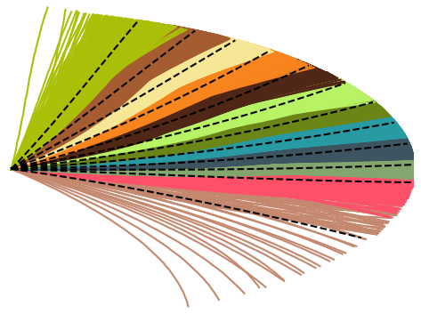
The optimization method above requires us to evaluate the objective function for each available control action not yet within across all dataset paths to determine which control action is best to add. However, this is computationally expensive. In addition, real world data often contains many similar paths. This is because there are often a limited number of ways to navigate a given scenario, and certain ways are more common than others. To alleviate these issues, we first cluster the dataset using the K-means algorithm[24]. To measure the distance between paths, we use the pointwise Euclidean norm[14]. An example of a clustering result is shown in Figure 5.
After clustering, we bias our search process based on how well our learned control set is currently matching each path cluster. Initially, each cluster has a large, equal weight. Our optimization algorithm proceeds as follows:
Control Set Optimization
- 1.
Select a path cluster according to the selection weights, and randomly sample a subset of the path cluster and a subset of control actions.
- 2.
Compute the optimization objective for these subsets, adding each control action individually to and calling Algorithm 1 for each path in the cluster subset.
- 3.
Add the control action that decreases the objective the most to permanently. Terminate if no control action improved the objective.
- 4.
Update the cluster selection weights with the resulting value of the optimization objective. Return to 1).
This method focuses our optimization on clusters that are poorly matched. Through this process, the optimization runs faster, and is more likely to match all types of paths present in the dataset, rather than the most common ones.
IV Results
To evaluate our method, we devised three experiments. The first two used data from human-driven trajectories around a roundabout, and the third used synthetic paths created through randomly generated scenarios. In all three experiments, we performed an 85-15 split of the dataset between the training and test sets. The algorithms were written in Julia. The source code for the experiments can be seen at https://github.com/rdeiaco/learning_lattice_planner. For all experiments, the dense initial control set was a set of cubic spirals[25] arranged in a cone, generated for all . The endpoints of the control actions in the cone had a range of values between 0.4m and 4.0m, a range of values between -2.0m to 2.0m, and values within [0, , , , , ]. These angles were chosen because they encourage straight line traversal between vertices in the lattice graph, which improves path quality[1]. The initial dense control set is shown in Figure 6a.
In each experiment we compared the performance of our learning algorithm to the state-of-the-art lattice computation algorithm[7]. The learning algorithm was run with and . These values were determined by logarithmically spaced grid search. Values of larger than this were found to generate control sets that were too sparse with poor manoeuvrability. Swath-based collision checking was performed using a rectangular vehicle footprint of length 4.5m and width 1.7m. Since the goal was not necessarily reachable in the lattice graph, the lattice planner instead searched for goal points that minimized the distance and heading difference from this goal.


IV-A Experimental Setups
Experiment 1: Roundabout Scenario
The first experiment involved taking 213 paths in a roundabout dataset11 1 Dataset obtained with permission from DataFromSky. The paths were extracted from cars driving through a European roundabout. The paths ranged in length from 27.6 to 87.4m.and sampling them at a constant arc length step size. The roundabout is illustrated in Figure 7a. The training portion of the dataset was then sliced into 10m arc length slices using a sliding window with a 1m step size. These slices were then taken as input to the clustering and optimization algorithms. This slicing method allows us to extract as much information as possible from the dataset[26]. To evaluate our learned control sets, we then took the test portion of our dataset and constructed scenarios from each path. To do this, we took the test set path as the lane centerline, with lateral offsets from the path forming the lane boundaries in an occupancy grid. Finally, we used the endpoint of the test set path as the goal, as well as the occupancy grid, and ran a lattice planner using each generated control set to compare the quality of each control set’s planned paths.


Experiment 2: Roundabout Lane Change Scenario
The second experiment also involved the same training paths from the roundabout dataset, except this time we added a second lane to the test set by extending the lateral offset forming the lane boundaries. Rather than the goal being to travel to the end of the original lane, the goal was changed to be the end of the adjacent lane. This meant that the planner was required to perform a lane change, in order to demonstrate that the learned control set could generalize to a situation not explicitly present in the training set. The direction of the lane change was equally distributed between a left and right lane change. Otherwise, scenario generation was the same as in Experiment 1.
Experiment 3: Synthetic Double Swerve Scenario
For the third experiment, we generated 100 different lane structures by randomly sampling clothoids of varying length and curvature connected to straightaways of varying length. Next, a second lane was then added, along with an obstacle in the first lane. The goal of this experiment was for the planner to perform a double swerve manoeuvre to avoid the obstacle. We then used the motion planner currently used on the University of Waterloo Autonomoose self-driving car[27] to generate the training set of synthetic paths. This dataset is shown in Figure 7b.
| Experiment 1 | Dense | DL[7] | ||
| Control Set Size | 311 | 194 | 64 | 109 |
| Planning Speedup Ratio | 1.00 | 1.82 | 6.40 | 3.49 |
| Matching Differential (31 Scenarios) | - | -1 | +9 | +11 |
| Experiment 2 | ||||
| Control Set Size | 311 | 194 | 65 | 109 |
| Planning Speedup Ratio | 1.00 | 1.73 | 7.46 | 3.83 |
| Matching Differential (31 Scenarios) | - | +7 | +13 | +23 |
| Experiment 3 | ||||
| Control Set Size | 311 | 194 | 57 | 83 |
| Planning Speedup Ratio | 1.00 | 1.90 | 7.73 | 4.70 |
| Matching Differential (15 Scenarios) | - | +5 | +11 | +13 |
IV-B Experimental Results
The results of all 3 experiments are shown in Table I. Here we can see that the learned control sets are significantly smaller than both the dense control set as well as the control set formed after performing the DL[7] lattice computation algorithm, illustrated in Figure 6. Notably, this results in up to an approximately 7.5x planning speedup over the dense set and up to a 4.31x planning speedup over the DL[7] set when executing the test set.
To measure how well each control set matched the dataset in terms of driving style, we computed the curvature at each point along each planned path and dataset path as a proxy for the steering function, as discussed in Section I-B. Next, we computed the maximum difference in curvature between each path point along the planned path and the dataset path. We call this the curvature matching score. Afterwards, we compare these curvature matching scores across the planned paths for each control set. The value in the table reports the number of times a planned path had a lower maximum curvature deviation than the dense set’s planned path; a positive number denotes the control set was better at matching more often than the dense set, and negative the opposite. A sample comparison between the DL control set and the control set is given in Figure 8.
From this, we can see that the learned control sets match the driving style (measured by curvature) of the dataset more closely than both the dense and DL[7] control sets, while also offering faster planning times. In addition, we can see that as gets smaller, the planned paths more closely match the data, at the cost of a larger control set and slower planning times.

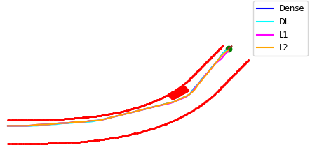
Figure 9 shows a sample planning run from Experiment 3, comparing all 4 control sets. The red box denotes the obstacle for the scenario. We can see that all 4 planners were able to complete a plan to the goal state equally well, which shows that the learned planners had no loss of manoeuvrability.
V Conclusions
This work presents a novel method for learning a lattice planner control set from a dataset of paths for a particular application. We demonstrated its efficacy through experiments involving real and synthetic data. The learned control sets are able to plan more quickly than the state of the art control set generation technique, and they better capture the driving style of the dataset during the planning process. In the future, we would like to explore combining learning the structure of a lattice planner with learning the lattice planner’s search heuristic, to see if lattice planner performance can be improved even further for specific applications. We would also like to extend this algorithm to handle trajectories rather than paths.
-A Proof of Theorem 1
We begin by proving correctness. To do this, we use induction on the vertices processed from , as well as the fact that the vertices are processed in topological order.
Induction Assumption. For each vertex processed from each , we have that the cost assigned to is the minimal possible on any path from the origin to , when comparing said path to to the subpath
Base Case. The origin is the first processed vertex, and since starts at the origin, is zero, which is the correct distance.
Induction. Now, assume every processed vertex satisfies the induction assumption. Suppose vertex is the current vertex to be processed. Since the algorithm processes vertices in topological order, all potential predecessors of have already been processed, and therefore satisfy the induction assumption. By the dynamic programming update, taking to be the set of predecessors of , we then have that
Now, let in denote the optimal predecessor of . By the update, we have that
thus the induction assumption holds for .
For runtime, Algorithm 1 iterates through a topological ordering of the search graph, which can be thought of as groups of at most vertices. For each vertex in the topological ordering, we perform a dynamic programming update for each control action available to it. Across all headings, the total number of control actions available to any particular vertex is , which in aggregate gives us . Each dynamic programming update calculates for an edge, which takes time. Combining, this gives us a computational complexity of .
-B Practical Considerations
Arc Length Relaxation. Since the lattice control actions connect vertices in the lattice graph, a realistic application of this method would require a small line segment length , which would in turn increase the size of required in each path matching calculation. To remedy this, we relax the requirement that each control action has an arc length that is integer-divisible by . This potentially results in a leftover portion of each control action that would be left out of the closest path calculation. We overcome this by checking if the leftover portion of the control action is greater than or equal to half of . If it is, then we treat it as a full line segment for computation. Otherwise, we ignore it. In practice, using a that is a of allows for good results.
Optimization Initialization. Finally, we initialize the learned control set with a single short, straight action for each possible initial direction, to ensure that the closest path algorithm can make forward progress when it encounters a point with any particular heading.
References
- [1] M. Pivtoraiko and A. Kelly, “Generating near minimal spanning control sets for constrained motion planning in discrete state spaces,” IEEE/RSJ IROS, 2005.
- [2] M. Pivtoraiko, I. A. Nesnas, and A. Kelly, “Autonomous robot navigation using advanced motion primitives,” IEEE Aerospace Conference, 2009.
- [3] M. Pivtoraiko, R. A. Knepper, and A. Kelly, “Differentially constrained mobile robot motion planning in state lattices,” Journal of Field Robotics, vol. 26, no. 3, pp. 308–333, 2009.
- [4] M. Mcnaughton, C. Urmson, J. M. Dolan, and J.-W. Lee, “Motion planning for autonomous driving with a conformal spatiotemporal lattice,” IEEE ICRA, 2011.
- [5] T. Gu, “Improved trajectory planning for on-road self-driving vehicles via combined graph search, optimization and topology analysis,” Ph.D. dissertation, Carnegie Mellon University, 2017.
- [6] J. Ziegler and C. Stiller, “Spatiotemporal state lattices for fast trajectory planning in dynamic on-road driving scenarios,” IEEE/RSJ IROS, 2009.
- [7] M. Pivtoraiko and A. Kelly, “Kinodynamic motion planning with state lattice motion primitives,” IEEE/RSJ IROS, 2011.
- [8] B. Ichter, J. Harrison, and M. Pavone, “Learning sampling distributions for robot motion planning,” arXiv preprint arXiv:1709.05448, Sep 2017.
- [9] S. Choudhury, M. Bhardwaj, S. Arora, A. Kapoor, G. Ranade, S. Scherer, and D. Dey, “Data-driven Planning via Imitation Learning,” ArXiv e-prints, Nov. 2017.
- [10] M. Bhardwaj, S. Choudhury, and S. Scherer, “Learning heuristic search via imitation,” CoRR, vol. abs/1707.03034, 2017. [Online]. Available: http://arxiv.org/abs/1707.03034
- [11] B. Paden, V. Varricchio, and E. Frazzoli, “Verification and synthesis of admissible heuristics for kinodynamic motion planning,” IEEE Robotics and Automation Letters, vol. 2, no. 2, pp. 648–655, 2017.
- [12] T. Zhang, G. Kahn, S. Levine, and P. Abbeel, “Learning deep control policies for autonomous aerial vehicles with MPC-guided policy search,” IEEE ICRA, 2016.
- [13] G. Yuan, P. Sun, J. Zhao, D. Li, and C. Wang, “A review of moving object trajectory clustering algorithms,” Artificial Intelligence Review, vol. 47, pp. 123–144, Mar 2016.
- [14] J. Chen, R. Wang, L. Liu, and J. Song, “Clustering of trajectories based on Hausdorff distance,” International Conference on Electronics, Communications and Control (ICECC), 2011.
- [15] T. Eiter and H. Mannila, “Computing discrete Fréchet distance,” Technische Universitat Wien, Tech. Rep. CD-TR 94/64, 1994.
- [16] C. Wenk, “Shape matching in higher dimensions,” Ph.D. dissertation, FU Berlin, 2003.
- [17] D. Chen, A. Driemel, L. J. Guibas, A. Nguyen, and C. Wenk, “Approximate map matching with respect to the Fréchet distance,” Proceedings of the Thirteenth Workshop on Algorithm Engineering and Experiments (ALENEX), pp. 75–83, 2011.
- [18] G. Oriolo, M. Ottavi, and M. Vendittelli, “Probabilistic motion planning for redundant robots along given end-effector paths,” IEEE/RSJ IROS, 2002.
- [19] R. M. Holladay and S. S. Srinivasa, “Distance metrics and algorithms for task space path optimization,” IEEE/RSJ IROS, 2016.
- [20] C. C. Macadam, “Understanding and modeling the human driver,” Vehicle System Dynamics, vol. 40, no. 1-3, pp. 101–134, Jan 2003.
- [21] P. Polack, F. Altche, B. Dandrea-Novel, and A. D. L. Fortelle, “The kinematic bicycle model: A consistent model for planning feasible trajectories for autonomous vehicles?” IEEE Intelligent Vehicles Symposium, 2017.
- [22] M. N. Pivtoraiko, “Differentially constrained motion planning with state lattice motion primitives,” Ph.D. dissertation, Carnegie Mellon University, 2012.
- [23] C. Wenk, R. Salas, and D. Pfoser, “Addressing the need for map-matching speed: Localizing global curve-matching algorithms,” 18th International Conference on Scientific and Statistical Database Management, 2006.
- [24] K. P. Murphy, Machine learning: a probabilistic perspective. MIT Press, 2012.
- [25] A. Kelly and B. Nagy, “Reactive nonholonomic trajectory generation via parametric optimal control,” The International Journal of Robotics Research, vol. 22, no. 7, pp. 583–601, Jan 2003.
- [26] F. Altche and A. D. L. Fortelle, “An LSTM network for highway trajectory prediction,” IEEE ITSC, 2017.
- [27] Y. Zhang, H. Chen, S. L. Waslander, T. Yang, S. Zhang, G. Xiong, and K. Liu, “Toward a more complete, flexible, and safer speed planning for autonomous driving via convex optimization,” Sensors, 2018.