Implicit Regularization in Over-parameterized Neural Networks
Abstract
Over-parameterized neural networks generalize well in practice without any explicit regularization. Although it has not been proven yet, empirical evidence suggests that implicit regularization plays a crucial role in deep learning and prevents the network from overfitting. In this work, we introduce the gradient gap deviation and the gradient deflection as statistical measures corresponding to the network curvature and the Hessian matrix to analyze variations of network derivatives with respect to input parameters, and investigate how implicit regularization works in ReLU neural networks from both theoretical and empirical perspectives. Our result reveals that the network output between each pair of input samples is properly controlled by random initialization and stochastic gradient descent to keep interpolating between samples almost straight, which results in low complexity of over-parameterized neural networks.
1 Introduction
Deep neural networks (DNNs) have achieved high performance in application domains such as computer vision, natural language processing and speech recognition. It is widely known that neural networks (NNs), which are very often used in the over-parameterized regime, generalize well without overfitting [36, 54]. However, the reason is not clear yet, and related questions remain largely open [40, 24]. Recent works have shown that with over-parameterization and random initialization, stochastic gradient descent (SGD) can find the global minima of NNs in polynomial time [13, 2], but trained network behavior in input data except for training samples is still not well-understood, and seems to be relevant to generalization in deep learning [51].
It has been known that a NN with i.i.d. random parameters can be equivalent to a Gaussian process, in the limit of infinite network width [34, 23, 30]. NNs often have significantly more parameters than samples in practice, and increasing the number of parameters can lead to a decrease in generalization error [6, 7]. It has been shown that the expressive power of NNs grows exponentially with depth for example by investigation into the number of linear regions [32, 49], analysis using Riemannian geometry and mean field theory [41], and study using tensor decomposition [11]. If the enormous expressive power is not controlled, deep learning architectures with large capacity will not generalize properly. However, these large NNs often generalize well in practice, despite the lack of explicit regularization. It is considered that implicit regularization plays a crucial role in deep learning and prevents the NN from overfitting [54, 46, 24].
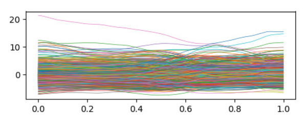
In order to estimate variations of NN derivatives with respect to input parameters, we define the gradient gap deviation and the gradient deflection, and investigate how implicit regularization works in ReLU activated neural networks (ReLU NNs) from both theoretical and experimental perspectives. Our result reveals that although the NN derivatives between each pair of input samples seem to change almost randomly, ReLU NNs interpolate almost linearly between the samples because of small variations of their derivatives (See Figure 1). In other words, we show that the NN output between the samples is properly controlled by weight initialization and SGD to keep connecting the samples almost straight, which results in low complexity of over-parameterized NNs. This result is consistent with the theoretical analysis and the experiments [33, 4, 24].
 (a) output on linear input path
 (b) gradient on linear input path
|
One key challenge in the behavior of NNs is that
the corresponding output functions and training objectives
are non-smooth due to the ReLU activation.
Whereas calculation of the network curvature and the Hessian matrix
w.r.t. input variables are necessary so as to make the evaluation of
such geometric complexity of ReLU NNs between each pair of input samples,
it is difficult to estimate them because the second order derivatives
cannot be defined as functions in .
Even though the input changes linearly,
the ReLU NN output changes piecewise linearly
and has many non-differentiable points
(break points)11
1
Strictly speaking, the NN output does not have gradient everywhere due to the non-smoothness of ReLU..
According to [1]:
One may naively think that since a ReLU network is infinite-order differentiable everywhere except a measure zero set, so we can safely ignore the Hessian issue and proceed by pretending that the Hessian of ReLU is always zero. This intuition is very wrong. (p.15)
All information about network variations is ingeniously encoded into the set of the break points caused by activation of ReLU, which has measure zero. We should analyze the behavior of the network output in an open neighborhood of this zero measure set to decode its global geometric information. In order to define alternatives to the network curvature and the Hessian matrix, it is necessary to characterize gradient gaps, that is, the slope changes at break points. Accordingly, we model the NN derivative (NN gradient) as a random walk bridge [26] on a linearly interpolating path between each pair of input samples (linear input path) to express quantitatively the global variations of NNs. By leveraging the random walk bridge, we investigate how the NN gradient changes as the input sweeps along the linear input path.
In the same line, the work in [6]
introduces a random walk for the gradient of a single hidden
layer network to show the gradient converges to Brownian motion
in the limit of infinite network width.
The work in [42, 37]
analyzes trajectory length and the number of linear regions,
which measure how the NN output (not the NN gradient) changes
as the input sweeps along a one-dimensional path,
and find that the trajectory length grows exponentially with depth.
Comparing with these results,
we present theoretical estimates of the gradient gap deviation
and numerical calculations of the gradient deflection,
and evaluate random variations of NN gradients statistically
to study the effect of implicit regularization by
random initialization and SGD.
These estimates depend only on
the feedforward map from input to output,
thus can be applied to a wide range of standard architectures
(e.g., VGG [44] and ResNet [18]).
Main Contributions
- •
We model a ReLU NN gradient w.r.t. input variables on a linear input path as a random walk bridge, and define the gradient gap deviation (7), that is, the standard deviation of NN gradient gaps between samples.
- •
We define the gradient deflection (8) as the amount of global variations of a ReLU NN between samples. Our result shows that the standard network models (MLP, VGG and ResNet) on the standard datasets (MNIST, CIFAR10 and CIFAR100) have small gradient deflection between samples (i.e., they interpolate almost linearly between samples), and also reveals that one of the mechanisms of implicit regularization by SGD is to keep gradient gaps to be small.
- •
We show that for the standard DNN models, the difference between the gradient gap deviation and the gradient deflection is relatively small, that is, the NN gradient is probably close to a random walk bridge on the linear input path.
- •
We also estimate the NN output itself and experimentally investigate the difference between the output variations on the linear input path and the mean margin at each pair of samples, which relate to the observed performance.
Notation. We use to denote . Let us denote the Euclidean norms of vectors by , and the spectral norms of matrices by . Let us denote the indicator function for event by .
2 Preliminaries
Consider an -layer fully-connected feedforward NN with units in each hidden layer. An activation function ReLU is given by , and for a vector , we define . The activation of hidden units and the output of each layer are given by
| (1) |
where is the input to the network, , , and are the weight matrices. For the input and the weight matrices , the NN output is also denoted by . Let us define indicator matrix , the diagonal elements of which are activation patterns ( or ) at each layer , as follows: For ,
| (2) |
Since the ReLU activation is positive homogeneous, we obtain the following equality:
| (3) |
For simplicity, we denote by the set of indicator matrices
.
We assume the following weight initialization [17]:
| (4) |
3 Random Walk Bridge for ReLU NNs
In this section, we define the gradient gap deviation and the gradient deflection on each NN, and show their theoretical estimates and experimental studies. We evaluate the estimates on three canonical machine learning datasets: MNIST [22], CIFAR10, and CIFAR100 [21] in our experiments.
3.1 Fully-connected Feedforword NNs (MLPs)
Now we consider a fully-connected feedforward NN (MLP) with ReLU activation for -classes classification, and show that the NN gradient between samples can be regarded as a random walk bridge.
We denote by and respectively the training inputs and the labels, where and . For weight matrices and an input , we denote by the NN output (1). The target function in learning is the cross entropy loss over the softmax defined as follows:
We randomly choose from training data or test data, and denote a direction vector by . We define a linear interpolation between and by , which is called the linear input path. We estimate the variation of the NN output pattern on the linear input path . Since the number of classes in the dataset is , is a -dimensional vector . We will link the directional derivative of each component function to a random walk bridge. For , we define the NN output between two points as follows:
For simplicity, we denote by the NN output . We define the NN gradient between and as follows22 2 It can be defined as a function :
Here NN gradient is normalized such that it is independent of the length of a direction vector . In particular, if then is equal to an ordinary derivative .
Since is a piecewise linear function due to ReLU [6, 42], we can define nodes of (i.e., break points at which the sign of the input to ReLU is switched) as . Here, is the number of times breaks in the interval . For notational simplicity, we denote both ends of the interval by and respectively. The number of nodes is equivalent to how many times the input linear path passes through other linear regions. The total number of linear regions of the input space is studied as a measure to evaluate expressivity and approximating ability of NNs [32, 42, 49]. For a single hidden layer MLP with ReLU activation (i.e., ), we can estimate the number of nodes as follows. This estimate can be proved by using random initialization, over-parameterization and input randomness. Moreover, since over-parameterization and random initialization jointly restrict every weight vector to be close to its initialization for all iterations [13, 2], it follows that this estimate changes little even after training.
Theorem 3.1 (Estimate of Number of Nodes)
Consider a two-layer fully-connected NN with rectified linear units and -dimensional input. Let , be random vectors with i.i.d. entries , and let be a weight matrix of the first layer with i.i.d. entries . Then the number of nodes in the interval is in distribution identical to binomial distribution with trials and success rate.
Our experimental results show that the mean of the number of nodes is approximately half of the number of entire hidden units for an even deeper network.
For each interval and for each layer , we denote by the indicator matrix (2) on the linear input path. We also abbreviate as . The diagonal elements of show ReLU activation of layer in the interval . By definition, the indicator matrices are different from each other. Since is constant in each interval , is a linear function and is a constant function. For , we use to denote NN gradient. For each node , we define NN gradient gap as . This implies that
| (5) |
We define a probability measure as distribution of NN gradient gaps when choosing randomly, and denote by the variance of . We assume that the mean of is zero, and define as i.i.d. random variables from the probability distribution . Then we model the NN gradient as a random walk bridge generated by , which satisfies the following:
| (6) |
If gradient gaps are i.i.d. random variables, then is the random walk bridge satisfying the boundary conditions on and . For a standard random walk, the boundary value at one out of both ends is fixed. For a random walk bridge, the both end values are fixed, which is represented by a conditional probability. In this setting (6), the following theorem evaluates to what extent a random walk bridge deviates from a linear interpolation between the both ends.
Theorem 3.2 (Estimate of Gradient Gap Deviation)
Let be a random walk bridge (6) generated by a probability distribution with mean and variance , and let be a random walk bridge defined by . We define gradient gap deviation for distribution as follows:
| (7) |
Then the gradient gap deviation is equal to .
Using the gradient gap deviation, which attains the maximum value at the midpoint , we estimate stochastically the difference between a random walk bridge and the linear interpolation from one end to the other.
In contrast, we also define the difference between the NN gradient on the linear input path and a linear interpolation of both end values of the NN gradient: For the input samples and ,
Suppose and are chosen uniformly from a certain training or test dataset. Then we define deflection of the NN gradient (gradient deflection) by the following expectation:
| (8) |
Here the difference between the gradient gap deviation (7) and the gradient deflection (8) is corresponding to the one between the amount of change in the random walk bridge and the network output change in the actual case. Inspecting this difference enables us to statistically measure the extent to which the NN changes contrivedly. Then, since the distribution is determined by activation patterns of ReLU, we obtain the following estimate:
Theorem 3.3 (Estimate of Gradient Gap)
Consider an -layer fully-connected neural network with rectified linear units in each layer. If , with probability at least over the randomness of , then gradient gaps are in distribution almost identical to the combination of and .
 (a) Number of nodes
 (b) Gradient Gap Deviation
 (c) Gradient Deflection
|
First we show experimental observations of the two-layer MLPs in the initial state (without training). Figure 2 (a) shows that the number of nodes is approximately equal to its theoretical value . The values of gradient gap deviation and gradient deflection are small in Figure 2 (b) and (c). Even if the number of units increases, both values of gradient gap deviation and gradient deflection hardly vary. In particular, the theoretical value of gradient gap deviation (Theorem 3.2) for the two-layer MLPs in the initial state is as follows:
where is the number of hidden units, and is the input dimensions.
Normalization procedure for network output. If the variance of the output pattern (i.e., ) changes by training or network architecture, it is difficult to compare with other NN gradients . Weights are initialized randomly so that the variance of the input will not change in each layer [17]. It is known that much deeper NNs can be trained by intensifying such effect of initialization [52, 55]. In this work, we adopt the following method, which is the same as [12, 7, 25]: Without loss of accuracy in classification, we can replace the output with , where is an arbitrary fixed number for each input . Therefore, we define each fixed number for normalization of random walk bridge as follows: For each input , define as the norm of the output vector . In other words, we normalize the NN output by letting . Now using the normalized NN output enables us to estimate random walk bridge even if the weights change with SGD training steps.
Numerical finite difference approximations of derivatives.
As the number of units or the number of layers increases
the number of nodes becomes large and the length of each
interval becomes extremely short.
In particular, we cannot calculate precisely
the derivative of the output function
by subtracting in the short interval
owing to cancellation of significant digits
in GPU calculation using single precision floating point arithmetic.
Instead, we propose a method of replacing each ReLU activation layer with
indicator matrix (2),
and only need to calculate the product of the matrix
(See Appendix (9)).
Next we show that the complexity measures (the number of nodes, the gradient gap deviation and the gradient deflection) change with SGD training steps for two-layer MLPs with different number of units. We observe that the number of nodes converges relatively fast and does not change significantly in Figure 3 (a).
 (a) Number of nodes
 (b) Gradient Gap Deviation
 (c) Gradient Deflection
|
We investigate how randomly an MLP changes between samples. Let denote a random walk bridge (6) generated by the probability distribution . Figure 3 (b) and (c) show the gradient gap deviation of and the gradient deflection (i.e., deviation of actual gradient change of MLP: ) at midpoint with SGD training steps. Although in the above-mentioned figures we sample randomly a pair of from training data, we obtain the same result even when we sample randomly them from test data.
3.2 VGG and Residual Networks
Now we show that for VGG [44] and residual network (ResNet) [18, 19], the NN gradient between samples can be regarded as a random walk bridge. We also show experimental results of the gradient gap deviation and the gradient deflection.
Let us denote the output of VGG or ResNet by for weight matrices and an input sample . As with §3.1, we investigate the variation of the NN output between two input samples . Let be a linear interpolation , and be a direction vector . Then, by using the NN output , we similarly define and between two points as follows:
Let be the nodes of a piecewise linear function . The number of nodes corresponds to the number of linear regions intersecting the linear input path. The number of linear regions of deep models (VGG and ResNet) grows exponentially in and polynomially in , which is much faster than that of shallow models with hidden units [32, 43]. In contrast, our experimental results for VGG and ResNet show that the number of nodes is half of the number of entire hidden units or less. The number of nodes increases linearly rather than exponentially with the depth (the number of layers), which is completely different from linear regions. Thus, by Theorem 3.2, gradient gap deviation, which is the fluctuation of random walk bridge, is relatively small. Since in the over-parameterized setting, SGD learns a NN close to the random initialization, the number of nodes is proved to change little.
 (a) Number of nodes
 (b) Gradient Gap Deviation
 (c) Gradient Deflection
|
 (d) Number of nodes
 (e) Gradient Gap Deviation
 (f) Gradient Deflection
|
We also define a NN gradient at as for VGG or ResNet. For each node let , be a gap of NN gradients. If each is an i.i.d. random variable, then is a random walk bridge between . Let be the distribution of as the inputs are chosen randomly from training or test samples, and let be a random walk bridge (6) generated from i.i.d. random variables with the distribution . As with an MLP, the initial weights determine the gap distribution , and weights change little in the over-parameterized setting. Accordingly, also changes little.
First we show experimental results for VGG and ResNet in the initial state (without training) on MNIST, CIFAR10 and CIFAR100. Figure 4 (a) and Figure 5 (a) show that the number of nodes is only half of the number of entire hidden units over VGG and ResNet or less. Figure 4 (b-c) for VGG and Figure 5 (b-c) for ResNet show that the values of gradient gap deviation and gradient deflection are small (). Next, we make use of the normalized NN output to handle the weight change with training. Figure 4 (d) and Figure 5 (d) show the changes in the number of nodes between samples with SGD training steps. In order to calculate precise NN gradient and avoid cancellation of significant digits, we also use the method of replacing each ReLU activation layer with indicator matrix (2). In Figure 4 (e-f) and Figure 5 (e-f), we show the changes in the gradient gap deviation and the gradient deflection at midpoint with SGD training steps.
 (a) Number of nodes
 (b) Gradient Gap Deviation
 (c) Gradient Deflection
|
 (d) Number of nodes
 (e) Gradient Gap Deviation
 (f) Gradient Deflection
|
By measuring the difference between gradient gap deviation and gradient deflection, it is possible to estimate systematically the variations in output between samples in comparison with completely random state. In other words, the above difference indicates the degree of randomness of NN gradients. Figure 4 (e-f) and Figure 5 (e-f) show that NNs tend to be random between a pair of samples after enough training, which suggests that NNs become passive or do not control the network output between samples actively.
No matter how large the complexity and expressivity of deep models are, random variation of the models between samples keeps small , which results in smoothness between a pair of samples (Figure 4 (e-f) and Figure 5 (e-f)). This suggests that more expressive power of deep models than needed is restricted, which is thought to be one of revealed abilities of implicit regularization in the over-parameterized regime. We also compare the results on training data with the ones on test data in Appendix, which suggests that there is no large difference between training data and test data.
 (a) The 2-layer MLP on MINST
 (b) VGG C8L3 on CIFAR10
 (c) ResNet34 on CIFAR100
|
In order to estimate the generalization ability on a linear interpolation between each pair of training samples, we introduce the following pair margin : For the input sample , its correct label and the normalized output vector , we define as . This value is the margin [7], which measures the gap between the output for the correct label and other labels. Then let be an average of these two values: . This is corresponding to the value that interpolates the margin linearly at the midpoint of and (i.e., ).
Next, we introduce the following pair fluctuation as the amount of fluctuation of the NN output between two samples. Let us denote by , a pair of samples, and by the normalized NN output between two points . We define the pair fluctuation between the two points as the difference between the mid point value and the mean of edge values and : .
Figure 6 shows the changes in the pair margin and the pair fluctuation with SGD training steps. As the training progresses, the value of exceeds the one of , which suggests that the accuracy increases even at the midpoint of two training samples, and the relation between and is likely to be coupled with the validation accuracy.
4 Related Works
Recently, many works try to explain generalization of neural networks linked to random initialization and over-parameterization. Recent work has shown that the difference between the learned weights and the initialization is small compared to the initialization in the over-parameterized regime [53, 50, 24], and SGD can find global minima of the training objective of DNNs with ReLU activation in polynomial time [13, 2]. Our method was inspired by a line of work [3, 2], which presents a method of estimating weight variation and NN norm. The work in [1] explains implicit regularization for two-layer NNs without weight regularizer. Many recent works also study the importance of random initialization [15, 17, 29, 48, 47, 31, 14].
It was pointed out empirically that the generalization ability of over-parameterized NNs cannot be estimated properly in classic learning theory [36, 54], which triggered various research on generalization. The relationship between loss landscape and generalization [20, 12, 51, 10], and the degree of memorization and generalization [5] have revealed. Several different measures for the generalization capabilities of DNNs have been examined, and generalization bounds for NNs with ReLU activation have been presented in terms of the product of the spectral norm and the Frobenius norm of their weights [16, 35, 7, 4]. Theoretical analysis on generalization on over-parameterized NNs has been presented [39, 40].
The work in [45] shows that bounding the Frobenius norm of the Jacobian matrix, which is first-order derivatives, reduces the obtained generalization error. The work in [37] shows that NNs implement more robust functions in the vicinity of the training data manifold than away from it, as measured by the norm of the Jacobian matrix. While they use the norm of the Jacobian matrix to estimate generalization and sensitivity, we evaluate the gradient gap deviation and the gradient deflection corresponding to Hessian and curvature to see NN ability in a different light. We therefore find that although the NN derivative changes rather randomly between samples, it interpolates between samples linearly because the amount of its variation is small.
Some recent studies [27, 28, 8] indicate that the generalization error of a NN is small because a NN interpolates smoothly between a pair of samples. The work in [9, 46, 24, 38] uses low complexity of the solution found by SGD to explain the small generalization error of over-parameterized models measured by classification margin. However, without any additional assumption on the dataset structure and the network architecture, the direct reason why SGD can find smooth and low-complexity solutions is unknown. In the present work, we tackle this question, and show that in the general setting, SGD restricts gradient gap and the number of nodes to be small, and the NN output between samples is properly controlled by weight initialization and SGD to keep connecting samples almost straight.
The work in [6] demonstrates the connection between the gradients of a two-layer fully-connected NN and discrete Brownian motion (random walk). In this work, we model the NN gradient as a random walk bridge to estimate the amount of change in the network gradient, and explain the low complexity of the learned solution, as measured by gradient gap deviation and gradient deflection. The work in [42, 37] investigates trajectory length of a one-dimensional path, and finds that the trajectory length grows exponentially in the depth of the NN. In contrast, we stochastically estimate gradient variation between samples and show that the motion of the network gradient is probably close to a random walk bridge.
5 Discussion
We model the gradient of NN output between a pair of samples as a random walk bridge, and introduce the gradient gap deviation and the gradient deflection. Furthermore, we estimate the global variation of ReLU NNs between samples, and reveal that ReLU NNs interpolate almost linearly between samples even in the over-parameterized regime. For standard ReLU NNs (MLP, VGG and ResNet) and datasets (MNIST, CIFAR10 and CIFAR100), we measure these values and investigate how implicit regularization works. The experimental observations suggest that the gradient gap deviation and the gradient deflection are both small for at least the above networks, which means that the network output interpolates between samples almost linearly. NNs converge to small fluctuation depending on the dataset, because excessive complexity and a large degree of freedom due to over-parameterization are controlled by SGD properly (we also ensured this result is independent of whether we use Momentum SGD or vanilla SGD). In order to keep the NN fluctuation to be small, it is necessary to prevent the gradient gap and the number of nodes from being larger than needed. In other words, one of the mechanisms of implicit regularization by SGD seems to restrict the gradient gap and the number of nodes.
One of the interesting questions for future work is to prove that for more deep networks, the number of nodes is only half of the number of entire hidden units or less. Our work is a step towards theoretical understanding of implicit regularization by random initialization and optimization algorithm for neural networks, and the study of constitutive relations between generalization and implicit regularization is left for future work.
References
- [1] Zeyuan Allen-Zhu, Yuanzhi Li, and Yingyu Liang. Learning and generalization in overparameterized neural networks, going beyond two layers. arXiv preprint arXiv:1811.04918, 2018.
- [2] Zeyuan Allen-Zhu, Yuanzhi Li, and Zhao Song. A convergence theory for deep learning via over-parameterization. arXiv preprint arXiv:1811.03962, 2018.
- [3] Zeyuan Allen-Zhu, Yuanzhi Li, and Zhao Song. On the convergence rate of training recurrent neural networks. arXiv preprint arXiv:1810.12065, 2018.
- [4] Sanjeev Arora, Rong Ge, Behnam Neyshabur, and Yi Zhang. Stronger generalization bounds for deep nets via a compression approach. arXiv preprint arXiv:1802.05296, 2018.
- [5] Devansh Arpit, Stanisław Jastrzębski, Nicolas Ballas, David Krueger, Emmanuel Bengio, Maxinder S Kanwal, Tegan Maharaj, Asja Fischer, Aaron Courville, Yoshua Bengio, et al. A closer look at memorization in deep networks. arXiv preprint arXiv:1706.05394, 2017.
- [6] David Balduzzi, Marcus Frean, Lennox Leary, JP Lewis, Kurt Wan-Duo Ma, and Brian McWilliams. The shattered gradients problem: If resnets are the answer, then what is the question? arXiv preprint arXiv:1702.08591, 2017.
- [7] Peter L Bartlett, Dylan J Foster, and Matus J Telgarsky. Spectrally-normalized margin bounds for neural networks. In Advances in Neural Information Processing Systems, pages 6240–6249, 2017.
- [8] Mikhail Belkin, Alexander Rakhlin, and Alexandre B Tsybakov. Does data interpolation contradict statistical optimality? arXiv preprint arXiv:1806.09471, 2018.
- [9] Alon Brutzkus, Amir Globerson, Eran Malach, and Shai Shalev-Shwartz. Sgd learns over-parameterized networks that provably generalize on linearly separable data. arXiv preprint arXiv:1710.10174, 2017.
- [10] Pratik Chaudhari and Stefano Soatto. Stochastic gradient descent performs variational inference, converges to limit cycles for deep networks. In 2018 Information Theory and Applications Workshop (ITA), pages 1–10. IEEE, 2018.
- [11] Nadav Cohen, Or Sharir, and Amnon Shashua. On the expressive power of deep learning: A tensor analysis. In Conference on Learning Theory, pages 698–728, 2016.
- [12] Laurent Dinh, Razvan Pascanu, Samy Bengio, and Yoshua Bengio. Sharp minima can generalize for deep nets. arXiv preprint arXiv:1703.04933, 2017.
- [13] Simon S Du, Xiyu Zhai, Barnabas Poczos, and Aarti Singh. Gradient descent provably optimizes over-parameterized neural networks. arXiv preprint arXiv:1810.02054, 2018.
- [14] Raja Giryes, Guillermo Sapiro, and Alexander M Bronstein. Deep neural networks with random gaussian weights: A universal classification strategy? IEEE Trans. Signal Processing, 64(13):3444–3457, 2016.
- [15] Xavier Glorot and Yoshua Bengio. Understanding the difficulty of training deep feedforward neural networks. In Proceedings of the thirteenth international conference on artificial intelligence and statistics, pages 249–256, 2010.
- [16] Moritz Hardt, Benjamin Recht, and Yoram Singer. Train faster, generalize better: Stability of stochastic gradient descent. arXiv preprint arXiv:1509.01240, 2015.
- [17] Kaiming He, Xiangyu Zhang, Shaoqing Ren, and Jian Sun. Delving deep into rectifiers: Surpassing human-level performance on imagenet classification. In Proceedings of the IEEE international conference on computer vision, pages 1026–1034, 2015.
- [18] Kaiming He, Xiangyu Zhang, Shaoqing Ren, and Jian Sun. Deep residual learning for image recognition. In Proceedings of the IEEE conference on computer vision and pattern recognition, pages 770–778, 2016.
- [19] Kaiming He, Xiangyu Zhang, Shaoqing Ren, and Jian Sun. Identity mappings in deep residual networks. In European Conference on Computer Vision, pages 630–645. Springer, 2016.
- [20] Nitish Shirish Keskar, Dheevatsa Mudigere, Jorge Nocedal, Mikhail Smelyanskiy, and Ping Tak Peter Tang. On large-batch training for deep learning: Generalization gap and sharp minima. arXiv preprint arXiv:1609.04836, 2016.
- [21] Alex Krizhevsky and Geoffrey Hinton. Learning multiple layers of features from tiny images. Technical report, Citeseer, 2009.
- [22] Yann LeCun, Léon Bottou, Yoshua Bengio, Patrick Haffner, et al. Gradient-based learning applied to document recognition. Proceedings of the IEEE, 86(11):2278–2324, 1998.
- [23] Jaehoon Lee, Yasaman Bahri, Roman Novak, Samuel S Schoenholz, Jeffrey Pennington, and Jascha Sohl-Dickstein. Deep neural networks as gaussian processes. arXiv preprint arXiv:1711.00165, 2017.
- [24] Yuanzhi Li and Yingyu Liang. Learning overparameterized neural networks via stochastic gradient descent on structured data. In Advances in Neural Information Processing Systems, pages 8167–8176, 2018.
- [25] Qianli Liao, Brando Miranda, Andrzej Banburski, Jack Hidary, and Tomaso Poggio. A surprising linear relationship predicts test performance in deep networks. arXiv preprint arXiv:1807.09659, 2018.
- [26] Thomas M Liggett. An invariance principle for conditioned sums of independent random variables. Journal of Mathematics and Mechanics, 18(6):559–570, 1968.
- [27] Siyuan Ma, Raef Bassily, and Mikhail Belkin. The power of interpolation: Understanding the effectiveness of sgd in modern over-parametrized learning. arXiv preprint arXiv:1712.06559, 2017.
- [28] Hartmut Maennel, Olivier Bousquet, and Sylvain Gelly. Gradient descent quantizes relu network features. arXiv preprint arXiv:1803.08367, 2018.
- [29] James Martens. Deep learning via hessian-free optimization. In ICML, volume 27, pages 735–742, 2010.
- [30] Alexander G de G Matthews, Mark Rowland, Jiri Hron, Richard E Turner, and Zoubin Ghahramani. Gaussian process behaviour in wide deep neural networks. arXiv preprint arXiv:1804.11271, 2018.
- [31] Dmytro Mishkin and Jiri Matas. All you need is a good init. arXiv preprint arXiv:1511.06422, 2015.
- [32] Guido F Montufar, Razvan Pascanu, Kyunghyun Cho, and Yoshua Bengio. On the number of linear regions of deep neural networks. In Advances in neural information processing systems, pages 2924–2932, 2014.
- [33] Vaishnavh Nagarajan and J Zico Kolter. Generalization in deep networks: The role of distance from initialization. In NIPS workshop on Deep Learning: Bridging Theory and Practice, 2017.
- [34] Radford M. Neal. Bayesian Learning for Neural Networks. PhD thesis, University of Toronto, Dept. of Computer Science, 1994.
- [35] Behnam Neyshabur, Srinadh Bhojanapalli, David McAllester, and Nathan Srebro. A pac-bayesian approach to spectrally-normalized margin bounds for neural networks. arXiv preprint arXiv:1707.09564, 2017.
- [36] Behnam Neyshabur, Ryota Tomioka, and Nathan Srebro. In search of the real inductive bias: On the role of implicit regularization in deep learning. arXiv preprint arXiv:1412.6614, 2014.
- [37] Roman Novak, Yasaman Bahri, Daniel A Abolafia, Jeffrey Pennington, and Jascha Sohl-Dickstein. Sensitivity and generalization in neural networks: an empirical study. arXiv preprint arXiv:1802.08760, 2018.
- [38] Guillermo Valle Pérez, Ard A Louis, and Chico Q Camargo. Deep learning generalizes because the parameter-function map is biased towards simple functions. arXiv preprint arXiv:1805.08522, 2018.
- [39] Tomaso Poggio, Kenji Kawaguchi, Qianli Liao, Brando Miranda, Lorenzo Rosasco, Xavier Boix, Jack Hidary, and Hrushikesh Mhaskar. Theory of deep learning iii: explaining the non-overfitting puzzle. arXiv preprint arXiv:1801.00173, 2018.
- [40] Tomaso Poggio, Qianli Liao, Brando Miranda, Andrzej Banburski, Xavier Boix, and Jack Hidary. Theory iiib: Generalization in deep networks. arXiv preprint arXiv:1806.11379, 2018.
- [41] Ben Poole, Subhaneil Lahiri, Maithra Raghu, Jascha Sohl-Dickstein, and Surya Ganguli. Exponential expressivity in deep neural networks through transient chaos. In Advances in neural information processing systems, pages 3360–3368, 2016.
- [42] Maithra Raghu, Ben Poole, Jon Kleinberg, Surya Ganguli, and Jascha Sohl-Dickstein. On the expressive power of deep neural networks. arXiv preprint arXiv:1606.05336, 2016.
- [43] Thiago Serra, Christian Tjandraatmadja, and Srikumar Ramalingam. Bounding and counting linear regions of deep neural networks. arXiv preprint arXiv:1711.02114, 2017.
- [44] Karen Simonyan and Andrew Zisserman. Very deep convolutional networks for large-scale image recognition. arXiv preprint arXiv:1409.1556, 2014.
- [45] Jure Sokolić, Raja Giryes, Guillermo Sapiro, and Miguel RD Rodrigues. Robust large margin deep neural networks. IEEE Transactions on Signal Processing, 65(16):4265–4280, 2017.
- [46] Daniel Soudry, Elad Hoffer, Mor Shpigel Nacson, Suriya Gunasekar, and Nathan Srebro. The implicit bias of gradient descent on separable data. Journal of Machine Learning Research, 19(70), 2018.
- [47] David Sussillo and LF Abbott. Random walk initialization for training very deep feedforward networks. arXiv preprint arXiv:1412.6558, 2014.
- [48] Ilya Sutskever, James Martens, George Dahl, and Geoffrey Hinton. On the importance of initialization and momentum in deep learning. In International conference on machine learning, pages 1139–1147, 2013.
- [49] Matus Telgarsky. Benefits of depth in neural networks. arXiv preprint arXiv:1602.04485, 2016.
- [50] Russell Tsuchida, Farbod Roosta-Khorasani, and Marcus Gallagher. Invariance of weight distributions in rectified mlps. arXiv preprint arXiv:1711.09090, 2017.
- [51] Lei Wu, Zhanxing Zhu, and Weinan E. Towards understanding generalization of deep learning: Perspective of loss landscapes. arXiv preprint arXiv:1706.10239, 2017.
- [52] Lechao Xiao, Yasaman Bahri, Jascha Sohl-Dickstein, Samuel S Schoenholz, and Jeffrey Pennington. Dynamical isometry and a mean field theory of cnns: How to train 10,000-layer vanilla convolutional neural networks. arXiv preprint arXiv:1806.05393, 2018.
- [53] Bo Xie, Yingyu Liang, and Le Song. Diverse neural network learns true target functions. arXiv preprint arXiv:1611.03131, 2016.
- [54] Chiyuan Zhang, Samy Bengio, Moritz Hardt, Benjamin Recht, and Oriol Vinyals. Understanding deep learning requires rethinking generalization. arXiv preprint arXiv:1611.03530, 2016.
- [55] Hongyi Zhang, Yann Dauphin, and Tengyu Ma. Fixup initialization: Residual learning without normalization. arXiv preprint arXiv:1901.09321, 2019.
Appendix A Proofs
A.1 Proof of Theorem 3.1
By assumption we know that
, are random vectors with i.i.d. entries
, ,
and the weight matrix of the first layer is initialized with
.
Now for fixed , let us denote
the row of as
We know that with high probability, for large enough input dimension ,
We define input vectors of hidden units and as follows:
, .
Then we obtain
,
and the two random variables ( and ) are independent.
Thus, it indicates that the signs of input and
are also independent, and each sign is chosen with half probability.
This means that the number of coincidences of
the two signs, namely, #,
is in distribution identical to binomial distribution
with trials and success rate.
We complete the proof.
A.2 Proof of Theorem 3.2
By assumption we know that .
Then we obtain by simple calculation
We complete the proof.
A.3 Proof of Theorem 3.3
We define a linear interpolation of two points , which are chosen from training data or test data. For a parameter , let us denote the interpolation as and its direction vector as . We define a vector valued function .
Let us assume that is a nodes of , and is the indicator matrices (2) defined with respect to .
By the randomness of the weight matrices , for small enough , it can be shown that with probability , the difference between indicator matrices and is only one element of one indicator matrix of a certain layer (i.e., one element difference between and for some ).
Let us denote and . For simplicity, we assume that the difference between indicator matrices and is only one element difference between and .
For , let us denote . Then we have
Under the above assumption, we set and obtain
Since is linear on a small neighborhood of , the gradient at is equal to for small enough , and we obtain
| (9) |
where is the normalized vector.
Similarly, we know that is equal to the following:
This implies that the gradient gap at is as follows:
For small enough , only one element of the matrix is non-zero, and the value of the element is equal to .
Next, in order to estimate the gradient gap ,
using concentration inequalities,
we obtain the following estimate
(see Lemma 4.1 in [2]):
Lemma. If , with probability at least
over the randomness ,
for a fixed unit vector and with ,
we have
This Lemma implies that with probability at least over the randomness , we have
In the following, for a fixed unit vector , we will estimate the norm of the layer activation
(Remark: If , then is equal to the unit vector .)
By the assumption, except for the one element of the matrix , all elements of the matrix are equal to zero. Thus, without loss of generality, we assume that the diagonal element is not equal to zero.
This implies that the nonzero element of is equal to the component of . Then we have
We also define the column vector of :
By the assumption, we know that
By the definition of weight initialization of , we have .
We define . By the above lemma, we know that with probability at least ,
By definition of , we have .
This implies that each element of is in distribution identical to .
Taking into consideration the estimates mentioned above, we have with probability at least :
We complete the proof.