Output Feedback Controllers Based on a Bank of High-Gain Observers: Robustness Analysis Against Measurement Noise
Abstract
This paper analyzes output feedback control of a class of unknown nonlinear systems in the presence of measurement noise using multiple high-gain observers (MHGO). It is well-known that single high-gain observers (HGO) are not able to provide satisfactory performance when the system output is contaminated by noise. More specifically, there is a trade-off between the convergence speed of state estimation and the bound of steady estimation error in HGO when the output measurement is contaminated by noise. In the presented scheme, the output feedback controller utilizes the state estimation obtained from an appropriate combination of information provided by a bank of HGOs. The proposed strategy is capable of mitigating the destructive effects of measurement noise and speeding up the convergence process, and it does that because it introduces an extra design parameter. The performance recovery capabilities of MHGO-based controllers and the stability of the closed-loop system are discussed. Simulations are performed on an underwater vehicle system and a mechanical system to evaluate the performance of the MHGO-based controller. Furthermore, a detailed comparison between the MHGO-based controller and controllers based on conventional HGO, HGO with switching gain, and multi-observer approach is provided, which shows the superiority of the MHG-based controller over the other methods.
I Introduction
States of systems have a prominent role in control theory, and many different strategies are developed by using them. Since all of the system states are not measurable in practice, different observation schemes are presented in the control literature. However, most of the previous studies were confined to the systems with noise-free output to simplify the understudied problem. This assumption is not realistic since measurements are mostly contaminated by noise; not only does this cause unsatisfactory performance, but it may also push the closed-loop system into instability. Hence, it is necessary to investigate the robustness of observers and observer-based controllers [1]. If a priori knowledge exists about the plant, Kalman filter is known as a powerful tool for estimation purposes [2], [3]. In [4], a fusion estimation algorithm is presented in terms of linear matrix inequalities for a class of uncertain linear systems. This scheme is based on the assumptions that the uncertain part of the plant satisfies certain conditions and multiple sensors measure the output. In [5], an adaptive observer is designed for a class of nonlinear systems with known dynamics and noisy measurements, and the relation between the observation error and bound of measurement noise is derived. However, the assumption of availability of a priori knowledge about system dynamics is not always valid. Moreover, the control problem, which is more challenging than the state estimation problem, has remained intact in the works above.
On the other hand, high gain observers (HGOs) are well-known as powerful structures for state estimation of nonlinear systems. These observers are capable of handling system uncertainties and providing fast and accurate estimations if their gains are chosen sufficiently large [6]. For control purposes, it has been shown that by feeding sufficiently fast HGO-based state estimations into a globally bounded controller, the output feedback controller can recover the performance of the state feedback controller [7]. HGOs, having these nice features, have attracted a great deal of attention in the past few decades and have been widely used in systems and control theory [8, 9, 10]. However, conventional HGOs with large gains yield state estimations with substantial over/undershoots in the transient response, known as the peaking phenomenon. Such behavior may result in a closed-loop system with a finite escape time, and in turn, might destabilize the overall plant [11]. In some works, intelligent strategies, (e.g., fuzzy systems, neural networks, etc.) are employed to estimate the system uncertainties and that approximation is fed into the dynamical equation of the HGO-based structure [12], [13], [14]. Although such structures may be applicable to a wide class of systems, they do not necessarily provide a nice transient response, specially when the initial conditions are chosen arbitrarily. Because, it takes a relatively long time for the intelligent part to learn the system dynamics, and in turn, these approaches result in an oscillatory response which is an inherent drawback of single adaptive models/structures [15], [16], [17]. On the other hand, in the past few decades, it has been shown that multiple model-based typologies are capable of providing parameter/state estimations with improved transient response [18], [19], [20], [21], [22], [23]. In these approaches, multiple models are run simultaneously, and the final estimation is obtained either by switching between different models [19], [20], [21] or by combining the available information [22, 23].
In addition to the peaking phenomenon, another problem with the conventional HGOs is sensitivity to measurement noise [6]. That is because the basic idea behind the conventional HGOs is to differentiate the system output to get estimations of immeasurable states. Thus, the performance of HGO-based structures should be evaluated with extra attention since the effects of measurement noise will be greatly amplified by differentiating the system output. The impact of measurement noise on the state estimations of HGOs is discussed in [24], and it has been shown that the gain of observer should not be selected too large or too small. In general, there is a trade-off between measurement noise sensitivity and the convergence rate of state estimation [25]. However, in HGO-based feedback controllers, sufficiently fast reconstruction of system states is a must (before that the system states leave the region of attraction) [11]. In [26], a new HGO structure is proposed for nonlinear systems in the presence of noise. In this approach, a large gain is employed, initially, to estimate system states fast; then the observer gain is switched to a smaller value to get a better steady state behavior. Although the basic idea behind this observation strategy is valuable, determining the switching time and the transient peaks may become challenging.
As motivated above, we will investigate output feedback control problem of nonlinear systems in the presence of measurement noise. In this regard, a bank of HGOs are utilized for state estimation purposes, which enables us to improve the transient response of conventional HGOs. The employed observation strategy, MHGO, uses all the information gathered from various observers simultaneously, and a weighted summation of these observations is considered as the final estimation. The main contributions of the paper can be summarized as follows:
- •
It is shown that there exist some weights enabling us to estimate the system states accurately and to speed up the estimation process in the presence of noise. This re-parameterization introduces an extra design parameter to the problem; hence the need for a large gain, which is required in the conventional HGO, is mitigated.
- •
The output feedback control problem in the presence of measurement noise is addressed, and by using the Lyapunov’s direct method, it is proven that a semi-separation principle is valid when using the state estimations provided by the MHGO.
- •
The robustness analysis of the MHGO-based controller is discussed, and the conditions on the bound of measurement noise and observer gain are derived.
- •
Capabilities of the MHGO-based controller in recovering performance of the state feedback controller are shown, and its supremacy of with respect to controllers based on conventional HGO, HGO with switching gains, and multi-observer approach are provided via simulations.
The remainder of this paper is organized as follows: The system equation and the problem under consideration are stated in Section II. Section III includes some preliminaries about convex sets and the HGO as well as the structure of the MHGO and comments on its performance. The key results on robustness analysis of the closed-loop system when the MHGO-based estimations are fed into a controller are presented in Section IV. Section V provides simulation results, and finally Section VI summarizes the paper.
II System Description and Problem Formulation
Consider a class of nonlinear systems in canonical form,
| (1) |
where represents the system state vector, and and denote the system input and output, respectively. Furthermore, expresses the output measurement noise with an unknown upper bound of , i.e., , and is an unknown nonlinear function. To guarantee the uniqueness of the system solution, is assumed to be locally Lipschitz in its arguments over the domain of interest and zero in a compact positively invariant set [6]. By defining , , and as
one can rewrite the system dynamics (1) in the following compact form
| (2) |
The system dynamics (2) cover a wide range of practical systems including electrical systems, mechanical systems, chemical processes, etc. Moreover, many other systems, which are not in the canonical form, can be transformed into the above standard form by employing appropriate transformations.
It is assumed that if all the system states are measurable, the following state feedback controller is capable of making the closed-loop system uniformly asymptotically stable concerning set [6],
| (3) |
where and are locally Lipschitz in their arguments over the domain of interest and globally bounded functions of . Furthermore, let us denote an open connected subset of the corresponding region of attraction by . Note that the considered class of control signal (3) covers a wide range of control inputs. The control input can be designed using feedback linearizion approach, sliding mode technique, any adaptive approach (conventional or intelligent), etc. Thus, the analysis provided in the subsequent sections are valid regardless of the way that the controller has been designed. In other words, one can design a state feedback controller separately and then replace the system states by the MHGO-based state estimations.
The understudy control problem is more general than the stabilization of an equilibrium point. In other words, lots of control problems (e.g., regulation, tracking, etc.) can be treated by properly defining the set . For instance, the stabilization problem of the origin is a special case of the problem above in which .
Since the assumption of availability of all system states is not always feasible in practice, the aforementioned controller cannot be applied to all real-life processes. To relax this assumption, it is required to estimate the system states suitably and feed them back to the controller. However, in this case, the stability of the closed-loop system should be investigated carefully. In the subsequent sections, the assumption of availability of all system states is removed by utilizing an observer-based controller, and the robustness of the closed-loop system when the system output is contaminated by measurement noise is analyzed.
III Observation Structure
This section presents the structures of conventional HGO and MHGO. In addition, a brief comparison between these two state estimation strategies are provided to elucidate more on the advantages obtained from combining observations collected from different sources/observers.
III-A High-gain Observer
The dynamical equation of a single HGO is as follows:
| (4) |
where and . Function is a nominal model of function which is locally Lipschitz in its arguments, globally bounded in , and zero in . In addition, are chosen such that the real parts of all roots of polynomial lie in the open left-half plane. Such a selection ensures that is a Hurwitz matrix.
It is well-known that the single HGO (4) can estimate system state vector accurately by selecting sufficiently large gains. However, the classic HGO (4) suffers from two major issues:
- (i)
undesirable peaks exist in the transient response of the estimated states, and if they are fed into the controller, they may push the system into instability
- (ii)
In the following subsection, several HGOs with suitable initial conditions are run, and the collected state estimations are employed to estimate the system state vector in a manner such that the aforementioned issues are mitigated.
III-B Multiple High-gain Observers
In this section, the MHGO structure and its capabilities in providing reliable state estimations are presented. Since this structure utilizes some properties of convex sets, it is useful to present the following lemma.
Lemma 1
[27] Let be a convex subset of a linear space. Then, any element of the convex hull of , i.e., , can be expressed as where are constant terms and .
In order to provide state estimations using multiple HGOs, inspired by [22], the dynamical equation for MHGO strategy is considered as follows:
| (5) |
where , is the state estimation obtained from the th observer. Besides, represent estimations of constant parameters , and they are calculated such that the equality holds. Note that to be able to use Lemma 1, the number of observers should be larger than the number of state variables, i.e., . Regarding the parameters , the following lemma is considered.
Lemma 2
Consider the state estimation (5). Let the initial conditions be chosen such that lies in their convex hull. Then, there exist some positive constant terms , with such that the state estimation error depends on and .
Proof: In order to prove the preceding lemma, let us use the facts that are constant terms and , and derive the dynamical equation of error as follows:
By substituting (2) and (5) into the preceding equation, one can get
| (6) |
Now, let us define a scaled version of the estimation error as , where the matrix is defined as follows:
| (7) |
Taking the time derivative of the scaled error and using (6), one can get
| (8) |
where and
Consider the Lyapunov function candidate for system (8), where is a positive definite matrix whose the largest and the smallest eigenvalues are denoted by and , respectively. It is assumed that satisfies the Lyapunov’s equation, i.e.,
| (9) |
Taking the time derivative of and utilizing (8) and (9), yield
| (10) |
Due to the globally boundedness of function in the domain of interest, one has . Using this fact and performing some basic mathematical manipulations on (10), one can get
The preceding equation can be rewritten as
This equation implies that as long as
As a result, the set
is an invariant set for the system.
Using the fact that the initial conditions of observers, , are selected such that lies in their convex hull, there exist constant terms such that or equivalently (see Lemma 1), and in turn, . Therefore, the estimation error is initiated from inside of the invariant set ; furthermore, we have . According to these facts, it is valid to say that . By using the preceding inequality and , one can show that
| (11) |
Consequently, there exists a bounded term such that . It is worth mentioning that when there is no measurement noise, , the ultimate estimation error bound can become arbitrarily small by choosing small enough .
It is well-known that the stability and performance of observer-based control strategies greatly depend on the convergence rate of the observer. More clearly, as will be shown later, if the state estimation error enters an invariant set fast enough, the closed loop system is stable. As it was shown in Lemma 2, we have ; hence the following equality holds.
| (12) |
Now, let us define and substitute (12) and (5) into it. Thus, we get
By adding to and subtracting from the right-hand side of the preceding equality (), it is valid to conclude that
| (13) |
where and . It is clear that since the final estimation error is the multiplication of two estimation errors and , this observation error is capable of entering the invariant set very fast. In other words, this type of problem re-parameterization (converting the state estimation problem into estimation of constant parameters ) expedites the convergence process. To obtain estimations of , the following RLS algorithm is employed,
| (14) | ||||||
where , , , is the identity matrix, and is a positive constant. Furthermore, the th column of is defined as .
Remark 1: In conventional HGOs the state estimation process can be performed fast enough by choosing a sufficiently small value for design parameter . However, this results in large peaks in the transient response of the state estimation, known as peaking phenomenon, and makes the ultimate state observation error large. For MHGO, it was shown that the speed of observer depends on the convergence rate of and (see (13)). On the other hand, it is well-known that the convergence rate of individual observers (5), , and the RLS algorithm (14), , depend on and , respectively. Thus, the need for considering a very small value for can be relaxed. To get the desired state estimation performance, the parameter needs to be selected large for making the ultimate estimation error small as well as avoiding the peaking, and the parameter should appropriately be chosen for improving the transient response and expediting the convergence rate. In regard to the initial conditions , if there is no a priori knowledge about how close the initial condition of the th observer () is to the system states, one can set the initial weights equally, i.e., . In the case that a prior knowledge exists, then we will give a higher initial weight to the closest observer.
IV Robustness Analysis of MHGO in Feedback Control
It is well-known that performance of observer-based controllers are dictated by the utilized state estimation. Due to the advantages mentioned for the state estimation obtained from MHGO, such a estimation is used for control purposes in this section, and the robustness and stability analyses of the closed-loop system are fully discussed. In this case, one can feed the estimated system states into the control signal (3), and get the output feedback controller as
| (15) |
In the sequel, it will be shown that the MHGO-based control signal (15) is capable of recovering the performance of the state feedback controller.
To analyze the performance of the closed-loop system, first let us subtract (2) from (5) and get the error dynamics of each observer as follows:
| (16) |
Now, define a scaled version of the estimation error , where is as presented in (7). Taking the time derivative of the scaled error and utilizing (16), result in
| (17) |
By using the fact that and the definition of (5), one can write the scaled state estimation error as follows:
| (18) |
where the th column of is . Besides, by employing (17), it is straightforward to show that
| (19) |
To get the dynamical equation of , it is required to take the time derivative of (18), and employ (14), (17), (19). Thus, one can get
By employing the facts that , , and , one can rewrite the preceding equation as follows,
| (20) |
Now, let us employ (2) and (20) and write the system dynamics under the output feedback controller (15) as follows:
| (21) | ||||
| (22) | ||||
The obtained dynamical equations represent a system in the standard singularity perturbed form. In order to analyze the closed-loop system behavior, one needs to consider the following facts and lemma.
Fact 1: Because is a positive definite matrix and (see (14)), it is valid to conclude that is bounded.
Fact 2: Since the matrix is Hurwitz, the dynamical equation (19) results in a bounded term . In other words, there exist positive constants and such that .
Lemma 3
Consider the nonlinear function with positive constants , , and . Then, there exist , and such that for every and a given constant term , inequality holds for every .
Proof: To prove the lemma, we will first show that has only one minimum point at . Then, this fact will be utilized to prove the lemma.
To prove the first part, it will be first shown that has at most two roots. Then, all possible scenarios will be discussed in detail, and it will be concluded that has exactly one minimum point. In this regard, the partial derivative of with respect to can be taken as follows:
| (23) |
To find extrema of , one should set . Since , this is equivalent to setting the numerator of the preceding equation equal to zero, i.e., . In order to show that the number of roots of is at most two, will be checked. By performing some basic manipulations, one can get , which has only one solution at . Hence, sign of changes one time (from a negative value to a positive value), and in turn, it is valid to conclude that has at most two solutions.
Now, let us consider the following three possible cases: (i) has no solution (ii) has one solution (iii) has two distinct solutions. Let us check some properties of function and show that case (i) results in a contradiction. Since function has a negative slope for small values of (see (23)), , this function is indeed decreasing at the beginning. On the other hand, we have and . Thus, the slope of this function should change its sign at some points, which contradicts with the assumption of having no solution for , i.e., case (i). For case (ii), let us assume that denotes the root of . Since and both and tend to , is the minimum point of function . On the other hand, we have ; thus, in this case, the minimum occurs at . For case (iii), let us denote the two distinct roots of by and . Using a similar discussion presented for cases (i) and (ii), one can conclude that at least one of these distinct roots should be the minimum point of function , e.g., . For the other root, i.e., , since we assumed that , this point can be a minimum or a maximum or an inflection point of function . Because no function can have two consecutive minimum points (without having any maximum point in the between of them), cannot be a minimum point. It cannot be a maximum point either since this assumption contradicts with the fact that . On the other hand, is not an inflection point of function since for all bounded values of . In other words, case (iii) does not occur.
So far, it was proven that function has exactly one minimum at . To find the largest possible (less conservative) upper bound of , for a given constant , we need to check . Toward this end, by performing some basic manipulations on , one can conclude that the upper bound of noise, , should be less than or equal to . On the other hand, it is clear that if , then the equation has two solutions at and . Hence, the inequality holds for every .
The following theorem summarizes performance recovery of the singularly perturbed closed-loop system in the presence of measurement noise (refer to (21) and (22)).
Theorem 1
Let us consider the dynamical system (1) with the control input (3). If the system states are estimated using the observer (5) with the adaptive law (14), then for any compact set (where is an open connected subset of the region of attraction) and any compact set , there exist constants , and such that for every , , the solution , starting in , is bounded for all . Furthermore, the adaptive parameters and the individual observers estimations are bounded as well.
Proof: To prove the theorem, a positive invariant set will be derived for the system dynamics; then this will be utilized to ensure boundedness of all signals of the closed-loop system. Toward this end, let us consider the Lyapunov function candidate for system (22). Taking the time derivative of this function and substituting (22) and (9) into it, yield
| (24) |
Due to the globally boundedness of controller in its arguments and locally Lipschitz property of , one has over a domain of interest ( will be defined later). By using the preceding inequality and performing some basic mathematical manipulations on (24), one can get
where , , and . With regard to Facts 1 and 2, one can conclude that constant is a bounded term.
Now let us define the compact set
| (25) |
Outside of the above set, one has
By using Fact 2 and performing some basic manipulations on the preceding inequality, one can get
| (26) |
where . Note that by utilizing Facts 1 and 2, it is straightforward to conclude that the positive constant is bounded. By using inequality and (26), one has
| (27) |
where and denote the largest and smallest eigenvalues of the matrix . Taking integral over (27), results in
Since there exists a positive constant such that , one can get
| (28) |
Therefore, if is outside of the compact set (25), there exists a finite time after which will enter that set. To obtain a closed form for , the preceding inequality can be utilized to get
| (29) |
On the other hand, as long as the scaled state estimation error is inside , satisfies the following inequality
| (30) |
where . Hence, we showed that is bounded; however, the provided analysis were based on the assumption that . In the sequel, the analysis of this part is divided into two steps. First, we will ensure that when starts from inside of the set , will enter the set before that leaves , i.e., the provided analysis for is valid during this time interval. Second, it will be shown that is a positive invariant set, and in turn, and will remain inside the set thereafter.
Since the system dynamics are in the form of standard singularly perturbed systems [6], let us substitute into (21) and get
| (31) |
It is obvious that the reduced system is identical to the system under the state feedback controller (3), and in turn uniformly asymptotically stable with respect to the positively invariant set . According Lyapunov’s converse Theorem [6], there exists a Lyapanuv’s function and positive definite functions , , and for system (31) such that
| (32) |
where is an open connected subset of the region of attraction; moreover there exists such that .
Since the nonlinear function is locally Lipschitz function and is globally bounded over the set of interest , one has
where is a constant term. Taking integral over both sides of the preceding equation and using the fact that , yields . Moreover, we have ; thus the inequality implies that there exists such that is inside the set as long as . On the other hand, since tends to zero as (refer to (29)), there exists a constant term such that for we have . In other words, the scaled state estimation error enters the set fast enough before that the system states leave the set .
In the next step, it will be shown that if lies inside of the set , this pair will always remain there. In other words, is a positive invariant set. In this regard, by using the Lyapunov’s function for closed-loop system (21), one can get
Due to the fact that and the Lipschitz property of function over the domain of interest, it is valid to conclude that
where denotes the Lipschitz constant. Inside of the set the presented upper bound in (30) is valid; thus by utilizing this upper bound and , the preceding inequality can be rewritten as follows:
By setting in Lemma 3, we get for and . On the other hand, (obtained earlier for ensuring for all ) gives us an upper bound for the measurement noise, i.e., . Thus, the parameters , , and (used in the theorem) can be defined as , , and . Note that we showed that and for all . Hence, the set is a positive invariant set.
In summary, we proved that if and is outside of the set , then and will enter the set after units of time and will remain there for . This means that the solution is bounded.
To complete the proof and ensure boundedness of the other signals of the closed-loop system, it is needed to guarantee that . Toward this end, first let us show that each observer yields a bounded state estimation vector, i.e., . In this regard, one can rewrite dynamical equation (5) as
| (33) |
It was proven earlier that belongs to ; moreover is bounded as well. Therefore, equation (33) represents a linear system with Hurwitz matrix and bounded input , and in turn, .
To prove that , let us take integrate over (14) and get , and in turn, one has . Since , the preceding inequality can be rewritten as
| (34) |
As it was shown earlier ; thus belongs to . Using the preceding equality, Facts 1 and 2, and (34), one has , with where is a bounded constant. Hence, one has , and it is valid to conclude that .
V Simulation Results
In this section, two simulation results are presented to shed some light on the presented theoretical discussions. In the first simulation, a numerical example is considered and the obtained results for MHGO-based controller are compared with the conventional HGO-based approach as well as HGO with switching gain strategy [26]. In the second example, simulations are carried out on a mechanical system, and the superiority of the MHGO-based approach over conventional HGO-based schemes and multi-observer-based approaches is shown.
V-A Example 1: Underwater Vehicle
In this subsection, a simplified model of underwater vehicle in yaw with dynamical equation of
is selected for simulation purposes, where denotes the heading angle and is a positive constant. Let us assume that only the heading angle is measured and that measurement is contaminated by noise , i.e., . In this simulation, and the measurement noise, generated by Matlab uniform random number block with sampling time , is in the interval .
The control objective is to steer the heading angle to follow the sinusoidal wave . It is obvious that the state feedback controller can force the heading angle to track asymptotically. Since is not measurable, it should be reconstructed appropriately and fed into the above controller. As stated in the previous section, MHGOs are capable of providing such an estimation; hence they are used in this regard. For comparison purposes, simulations are also performed by utilizing the conventional HGO and the HGO with switching gain [26]. The basic idea behind the letter observation scheme, HGO with switching gain, is to switch from a small gain to a larger gain. More clearly, a small value for is employed in the beginning to get a fast response, then it is switched to a larger value to avoid large steady observation errors caused by the measurement noise [26].
The design parameters of the conventional HGO are selected as , , . Furthermore, the design parameters of the switching HGO change from , , to , , . Besides, it is assumed that the implemented control effort by the actuator is restricted by amplitude of . For the MHGO, to be able to run the adaptive laws (14), initial conditions of the RLS algorithm are selected as follows: , , and in turn . In addition, parameters and are set equal to the corresponding parameters of the conventional HGO. It is clear that the three approaches will eventually have , and in turn, all of them will affect the measurement noise with the same , which allows us to make an accurate comparison. Moreover, the initial conditions of the multiple observers, employed in MHGO, are required to be selected such that the initial system states, i.e., lie in their convex hull. Toward this end, three observers are initiated from and ; thus starts from . To make the simulation results more comparable, the initial condition of the conventional HGO and HGO with switching are set equal to as well.
The evolution of system states are depicted in Figs. 1 and 2. From these two figures, it is clear that the MHGO-based controller recovers performance of the state feedback controller faster than the two others. Also, due to the existence of the measurement noise on the system output , the controllers based on these observation strategies result in a bounded error. The state estimation process is also presented in Fig. 3 and 4. The obtained observation results are also in commensurate with the aforementioned discussions. These figures show that because a small value is considered for in the transient phase in switching gain approach, this scheme reconstructs system states faster than the conventional HGO. Nonetheless, as it is well-known in the control literature, such a selection yields to a large overshoot in the beginning of the estimation (see Fig. 5), which is not preferable in practice. While the obtained final estimation error for MHGO outperforms the other two approaches regarding the convergence rate and the avoidance of peaks since MHGO benefits from the advantages of using information/estimations gathered from various sources. Because, during the transient phase, the adaptive terms , , presented for re-parameterizing the observation problem and combining the estimations of each observer, assist the observation structure to result in better estimations (see Remark 1). Note that in the long run converge to their final values and since , MHGO behaves similarly to a HGO.
V-B Example 2: Connected Inverted Pendulums on Carts
Consider two inverted pendulums mounted on two carts and connected by a spring, as shown in Fig. 6. The governing dynamical equation of this mechanical system can be expressed as [28],
| (35) |
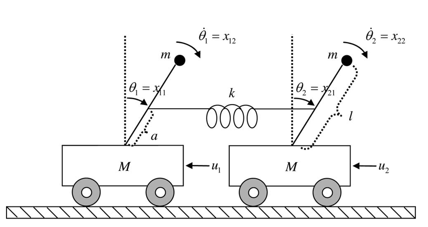
where and () represent the vertical angle of the th pendulum and its angular velocity , respectively, is the system state vector, denotes measurement noise, and with and . In this simulation, the following values are considered for system parameters: mass of pendulum kg, mass of cart kg, constant term , distance of the cart from the spring along with the bar m, length of pendulum m, spring constant N/m, and gravity acceleration m/s2.
In order to make the closed-loop system asymptotically stable and force its output vector to track the desired trajectory , the state feedback controller
which is saturated outside , is considered. Since it was assumed that only and are available, system states should be reconstructed appropriately. In the sequel, the state reconstruction process is performed using three different approaches, namely a single HGO, multi-observer, and MHGO, and capabilities of these observation strategies in recovering performance of the state feedback controller are compared.
Note that (35) is a multi-input multi-output (MIMO) system, hence, it is required to explain how the MHGO scheme can be employed for estimating the system states. Toward this end, by using the fact that (35) represents a special class of MIMO systems with two subsystems in normal form, one can employ two sets of MHGO for state estimation of the overall system. One MHGO uses to estimate and , and the other one employs for estimating and . Each set of MHGO has HGOs and the parameters estimations () obtained from the RLS algorithm (14). It is clear that the aforementioned approach can be easily extended to a class of MIMO nonlinear systems consisted of more than two () subsystems in normal form.
To carry out the simulations, the initial conditions of the system are considered as , and the measurement noise vector is generated by two uniform random number blocks of Matlab Simulink with the values restricted to the interval and sampling time . Note that from this point forward, the superscript is used to denote the state estimation of subsystem . In order to investigate the performance of conventional HGO-based controller, the state variables of each subsystem are estimated using a single HGO. For that, the design parameters and initial conditions of the th observers are selected as: , , , . In multi-observer approach, HGOs are run from various initial conditions to estimate states of the th subsystem, and at each time instant, the performance criterion obtained from is checked to find the best observer [20]. More clearly, the best observer for subsystem is chosen as , and in turn, the best estimation is (note that the observers do not cooperate). For multi-observer approach, first we will use three observers, , with initial conditions , , and to estimate the states of subsystem . Moreover, the rest of design parameters of the HGOs employed in the multi-observer method are chosen as same as the single HGO. To be able to make a reasonable comparison between the performance recovery of the MHGO-based controller and the aforementioned methods, the design parameters (i.e., , , ), the number of observers (i.e., ), and initial conditions (i.e., ) of MHGO are set equal to the ones selected for the multi-observer scheme. The RLS algorithm design parameters are considered as , . Thus, it is clear that such a selection results in . Furthermore, in multi-observer is set as ; hence all the observers have the same initial condition, i.e., .
The performance of the system states under the state feedback controller as well as the discussed output feedback controllers are illustrated in Figs. 7 and 8. These two figures obviously show that although the multi-observer-based controller yields a better response in comparison to the conventional HGO-based method, it does not outperform the MHGO-based controller. In other words, the MHGO-based controller has recovered the performance of the state feedback controller much faster than the other two methodologies. As discussed earlier and it is obvious from the zoomed parts in F-gs. 7 and 8, performance of the state feedback controller cannot be recovered perfectly due to the existence of measurement noise . Because of the space limitation and the fact the two subsystems behave similarly, only the observation errors of the first subsystem are provided (Figs. 9 and 10). According to these figures, one can easily see that the state estimation errors of MHGO strategy converge to a small neighborhood of the origin rapidly.
As mentioned in [20], [21], the multi-observer approach provides better results when the number of observers is increased. This implies that to assure that at least one of the models is sufficiently close to the plant, a quite large number of models is required. Hence, to make a more comprehensive comparison and show that the MHGO-based controller can outperform the multi-observer-based controller even when the number of observers are increased, another simulation with is carried out. In this simulation, all the design parameters are chosen the same as the previous scenario. For providing the initial conditions of observers for subsystem , four points , , , and are considered as the vertices of uncertainty region , within which the initial conditions of subsystem lies. Then, is sampled uniformly to obtain initial conditions for each set of observers. Simulation results are presented in Figs. 11-14. Figs. 11 and 12 clearly show that performance of the multi-observer-based approach is improved in comparison to the multi-observer with (see Figs. 7 and 8); however, it is computationally more expensive than that case. These figures also demonstrate that the MHGO-based control approach results in a better performance in this scenario as well. It is worth noting that in these simulations the MHGO-based controller with also outperforms the multi-observer-based controller with , which demonstrates the superiority of the MHGO-based strategy (refer to Figs. 7, 8, 11, 12). The obtained observations errors are also shown in Figs. 13 and 14, based on which it is clear that the MHGO scheme forces the observation errors to tend to a small neighborhood of the origin faster than other methods.
VI Conclusions
This paper investigates the analysis of the performance of MHGO-based controllers when the system output is contaminated by measurement noise. It is well-known that in this case, increasing the gain of a single observer deteriorates the steady state bound of estimation error. Hence, one cannot choose an arbitrarily large gain to speed up the transient response, which is necessary for control purposes. The MHGO utilizes the observations obtained from various sources and introduces new design parameters. In turn, it provides a suitable tool for solving the aforementioned trade-off in conventional HGO. The necessary conditions under which such a structure was capable of recovering performance of the state feedback controllers in the presence of measurement noise were derived, and the stability of the closed-loop system was investigated. Two simulations were carried out for comparison purposes and to validate the theoretical discussions.
Several simulations performed on various dynamical systems have shown that the MHGO-based control strategy has a larger region of attraction in comparison to the conventional HGO. The focus of our future work is to investigate this problem further and provide a rigorous proof for this claim.
References
- [1] J. C. Doyle and G. Stein, “Robustness with observers,” IEEE Trans. Autom. Contr., vol. 24, no. 4, pp. 607–611, 1979.
- [2] R. E. Kalman, “A new approach to linear filtering and prediction problems,” Fluids Eng., vol. 82, no. 1, p. 35–45, 1960.
- [3] Z. Xing, Y. Xia, L. Yan, K. Lu, and Q. Gong, “Multisensor distributed weighted kalman filter fusion with network delays, stochastic uncertainties, autocorrelated, and cross-correlated noises,” IEEE Trans. Syst. Man. Cybern.: Syst., vol. 48, no. 5, p. 716–726, 2018.
- [4] B. Chen, G. Hu, D. W. C. Ho, W. A. Zhang, and L. Yu, “Distributed robust fusion estimation with application to state monitoring systems,” IEEE Trans. Syst. Man. Cybern.: Syst., vol. 47, no. 11, pp. 2994–3005, 2017.
- [5] S. Battilotti, “Robust observer design under measurement noise with gain adaptation and saturated estimate,” Automatica, vol. 81, pp. 75–86, 2017.
- [6] H. K. Khalil and J. Grizzle, Nonlinear systems. Prentice hall New Jersey, 1996.
- [7] A. N. Atassi and H. K. Khalil, “A separation principle for the stabilization of a class of nonlinear systems,” IEEE Trans. Autom. Control, vol. 44, no. 9, pp. 1672–1687, 1999.
- [8] W. He, A. O. David, Z. Yin, and C. Sun, “Neural network control of a robotic manipulator with input deadzone and output constraint,” IEEE Trans. Syst., Man, Cybern.: Syst., vol. 46, no. 6, pp. 759–770, 2016.
- [9] K. Esfandiari, F. Abdollahi, and H. A. Talebi, “Adaptive control of uncertain nonaffine nonlinear systems with input saturation using neural networks,” IEEE Trans. Neural Netw. Learn. Syst., vol. 26, no. 10, pp. 2311–2322, 2015.
- [10] M. Shakarami, K. Esfandiari, M. A. Shamsi, and M. B. Menhaj, “High-gain observer-based identification scheme for estimation of physical parameters of synchronous generators,” 24th Iranian Conference on Electrical Engineering (ICEE), pp. 1422–1427, 2016.
- [11] F. Esfandiari and H. K. Khalil, “Output feedback stabilization of fully linearizable systems,” Int. J. Control, vol. 56, no. 5, pp. 1007–1037, 1992.
- [12] C. Li, S. Tong, and W. Wang, “Fuzzy adaptive high-gain-based observer backstepping control for siso nonlinear systems,” Info. Sci., vol. 181, pp. 2405–2421, 2011.
- [13] C. Ren, S. Tong, and Y. Li, “Fuzzy adaptive high-gain-based observer backstepping control for siso nonlinear systems with dynamical uncertainties,” Nonlinear Dyn., vol. 67, no. 2, pp. 941–955, 2012.
- [14] K. Esfandiari, F. Abdollahi, and H. A. Talebi, “Adaptive output feedback tracking control for nonaffine nonlinear systems,” in 2015 23rd Iranian Conference on Electrical Engineering. IEEE, 2015, pp. 976–981.
- [15] K. S. Narendra and A. Annaswamy, Stable adaptive systems. Prentice hall New Jersey, 1989.
- [16] K. Esfandiari, F. Abdollahi, and H. A. Talebi, “Stable adaptive output feedback controller for a class of uncertain non-linear systems,” IET Control Theory, Appl., vol. 9, no. 9, pp. 1329–1337, 2015.
- [17] K. Esfandiari, F. Abdollahi, and H. A. Talebi, “Adaptive near-optimal neuro controller for continuous-time nonaffine nonlinear systems with constrained input,” Neural Netw., vol. 93, pp. 195–204, 2017.
- [18] K. S. Narendra and K. Esfandiari, “Adaptive control of linear periodic systems using multiple models,” 2018 IEEE Conference on Decision and Control (CDC), pp. 589–594, 2018.
- [19] K. S. Narendra and O. A. Driollet, “Adaptive control using multiple models, switching, and tuning,” in Adaptive Systems for Signal Processing, Communications, and Control Symposium. IEEE, 2000, pp. 159–164.
- [20] R. Postoyan, M. H. Hamid, and J. Daafouz, “A multi-observer approach for the state estimation of nonlinear systems,” in 2015 54th IEEE Conference on Decision and Control (CDC). IEEE, 2015, pp. 1793–1798.
- [21] M. S. Chong, D. Nešić, R. Postoyan, and L. Kuhlmann, “Parameter and state estimation of nonlinear systems using a multi-observer under the supervisory framework,” IEEE Trans. Autom. Control, vol. 60, no. 9, pp. 2336–2349, 2015.
- [22] M. Shakarami, K. Esfandiari, A. A. Suratgar, and H. A. Talebi, “On the peaking attenuation and transient response improvement of high-gain observers,” 2018 IEEE Conference on Decision and Control (CDC), pp. 577–582, 2018.
- [23] Z. Han and K. S. Narendra, “New concepts in adaptive control using multiple models,” IEEE Trans. Autom. Control, vol. 57, no. 1, p. 78–89, 2012.
- [24] L. K. Vasiljevica and H. K. Khalil, “Error bounds in differentiation of noisy signals by high-gain observers,” Control Syst. Letters, vol. 57, no. 10, pp. 856–862, 2001.
- [25] H. Kwakernaak and R. Sivan, Linear Optimal Control Systems. New York: Wiley-Interscience, 1972.
- [26] J. H. Ahrens and H. K. Khalil, “High-gain observers in the presence of measurement noise: A switched-gain approach,” Control, Syst., Letters, vol. 45, no. 4, pp. 936–943, 2009.
- [27] I. J. Bakelman, Convex analysis and nonlinear geometric elliptic equations. Springer Science & Business Media, 2012.
- [28] W. Y. Wang, Y. H. Chien, and T. T. Lee, “Observer-based t–s fuzzy control for a class of general nonaffine nonlinears systems using generalized projection-update laws,” IEEE Trans. Fuzzy Syst., vol. 19, no. 3, pp. 493–504, 2011.