Long-lived circulating currents in strongly correlated nanorings
B. M. Schoenauer
Affiliation: Institute for Theoretical Physics, Center for Extreme Matter and Emergent Phenomena, Utrecht University, Princetonplein 5, 3584 CE Utrecht, The Netherlands
N. M. Gergs
Affiliation: Institute for Theoretical Physics, Center for Extreme Matter and Emergent Phenomena, Utrecht University, Princetonplein 5, 3584 CE Utrecht, The Netherlands
P. Schmitteckert
Affiliation: Institute for Theoretical Physics and Astrophysics, Julius-Maximilians University of Würzburg, Am Hubland, 97074 Würzburg, Germany
Affiliation: HQS Quantum Simulations GmbH, 76131 Karlsruhe, Germany
F. Evers
Affiliation: Institute of Theoretical Physics, University of Regensburg, 93040 Regensburg, Germany
D. Schuricht
Affiliation: Institute for Theoretical Physics, Center for Extreme Matter and Emergent Phenomena, Utrecht University, Princetonplein 5, 3584 CE Utrecht, The Netherlands
3 July 2019
Abstract
We study the time evolving currents flowing in an interacting, ring-shaped nanostructure after a bias voltage has been switched on. The source-to-drain current exhibits the expected relaxation towards its quasi-static equilibrium value at a rate reflecting the lead-induced broadening of the ring states. In contrast, the current circulating within the ring decays with a different rate , which is a rapidly decaying function of the interaction strength and thus can take values orders of magnitude below . This implies the existence of a regime in which the nanostructure is far from equilibrium even though the transmitted current is already stationary. We discuss experimental setups to observe the long-lived ring transients.
Introduction.—Isolated quantum systems, such as small molecules, feature a discrete set of energy levels. When brought to contact with two electrodes, a nano-junction can form and a current begins to flow. At weak coupling, the associated level broadening, , is still small as compared to the typical energy spacing, , of the isolated system. One might perhaps suspect that these energies by themselves set the only relevant time scales. But in fact a prominent exception is known, the Kondo phenomenon Hewson93, which occurs in a situation where is dominated by strong on-site repulsion between the charge carriers. This suppresses charge fluctuations but allows for spin fluctuations, leading to an emergent energy scale, the Kondo temperature , which is parametrically small compared to the native scales and .
In this work, we report another example of an emergent energy scale, ; it manifests in the relaxation of circulating currents in mesoscopic nanostructures. Like the Kondo temperature, the new scale is a many-body phenomenon, originating from interactions between particles on the nanostructure. However, the manifestation of the new relaxation rate requires the nanostructure to be brought out of equilibrium.
A sketch of a minimal model system that exhibits the novel scale is displayed in Fig. 1. Originally, similar ring-shaped devices served as a toy-models to study the interplay of interaction and interference BohrSchmitteckert12; Schmitteckert13 and to explain quantum-interference effects in transport through functionalised graphene ribbons Walz-14. The ring geometry supports stationary circulating (“orbital”) currents that can exceed the source-drain (“transport”) current by orders of magnitude at Fermi-energies situated close to a Fano-resonance.
Strong circulating currents in ring-shaped devices, Fig. 1, generically arise as transients after a voltage quench. They then carry an oscillating amplitude with a frequency resembling the lowest lying excitation gap of the nanostructure. We here report results from time-dependent density matrix renomalisation group (tdDMRG) Vidal04; WhiteFeiguin04; Daley-04; Schmitteckert04 simulations showing that in situations where the interaction is the dominating native scale of the nanoring, these oscillations can be very pronounced and very long-lived. They exhibit a lifetime that exceeds the transients in transport currents, , by orders of magnitude if the repulsive interaction becomes strong. The computational finding is complemented with perturbative arguments that explain this effect and clarify the relevant physical processes. In essence, the strong suppression of originates in a large energy gap between the two low-lying states and the rest of the spectrum on the nanoring (see Fig. 2), with ring current connecting the low-lying states. Possible experimental signatures of the effect proposed here are discussed. We note that in contrast to previously discussed MedenSchollwoeck03; Molina-03; RejekRamsak03 persistent ring currents driven by magnetic fields, the oscillating ring current we observe is a pure non-equilibrium effect.
Figure 1: Schematic representation of the nanostructure. The ring (red and green dots) is coupled by to left and right leads (blue dots). Spinless fermions can hop within the ring and leads with amplitude , the top site (site 2) on the ring is subject to the potential , and inside the ring a nearest-neighbour interaction is present.Figure 2: Time evolution of the transmitted and ring currents, and , evaluated using tdDMRG on the links and in Fig. 1. The recurrence time is indicated by the black arrow. While the transmitted current quickly relaxes to a stationary value, the ring currents show persistent oscillations with frequencies over the accessible times. The simulation parameters are , , , and .
Nanostructure.—The model associated with Fig. 1 is represented by the Hamiltonian describing the ring, the leads and their mutual coupling, respectively. The ring Hamiltonian is given by
(1)
with operators and creating/annihilating spinless fermions at site and denoting the corresponding density. The first term describes hopping of the fermions between nearest neighbours, while the second represents the repulsive nearest-neighbour interaction. The last term is an external potential at the top site which breaks the symmetry between the upper and lower path through the ring. The lead Hamiltonian reads
(2)
where and create and annihilate a spinless fermion at site in the lead . For simplicity we assume the hopping parameter in the ring and lead to be equal. Finally, the coupling between both subsystems is facilitated by
(3)
coupling the outer sites on the ring to the leads.
In the following we analyse the non-equilibrium currents in the nanostructure by three different methods: (i) tdDMRG simulations, (ii) a reduced density-operator transport theory (RDTT) Schoeller09; SaptsovWegewijs12, and (iii) mapping to an effective two-state nanostructure Bravyi-11.
Figure 3: Spectrum of the uncoupled ring relative to the ground-state energy . The ground state is a CDW state with particles, for the first excited state is also a CDW state with two particles. The corresponding particle densities are shown for . The observed oscillation frequencies of the ring currents match the energy difference between these two states. The higher excited states are obtained by adding or removing particles, with denoting the corresponding energies.
tdDMRG simulations.—First, we study the time evolution after a voltage quench using the tdDMRG algorithm BohrSchmitteckert07; Boulat-08; Kirino-08; DiasdaSilva-08; Heidrich-Meisner-09; Branschadel-10; Schwarz-18. Specically we use the time evolution scheme outlined in Refs. Schmitteckert04; Branschadel-10; supplement performing the evaluation of the time evolution via matrix exponentials within the framework of Krylov spaces. At times the system is prepared in the ground state of the model with an additional charge excess induced by a stationary gating with . At the gate is switched off, so the electrodes begin to discharge and currents start to flow through the system. We simulate the time evolution with finite leads which are long enough to be able to study the transient regime all the way into the quasi-stationary, non-equilibrium limit. Finite-size effects will interfere only at times exceeding the recurrence time , at which the electrons reach the boundary of the leads. (For details of the quenching protocol see Ref. Branschadel-10.) Here denotes the total number of sites, ie, the length of the leads is given by , and is the Fermi velocity of the lead electrons.
During the time evolution we determine the expectation values of the local currents and flowing in the leads and the impurity, respectively, where and are neighbouring sites. The local current densities after quenching are displayed in Fig. 2. The transport (“transmitted”) current initially fluctuates in response to the quench for times , where we use with the density of states in the leads as our time unit. After this transient the transmitted current appears to have reached a largely time-independent steady state in line with predictions from non-equilibrium Green function formalism Jauho-94; Tuovinen-13.
In contrast, for the local currents in the ring we observe a drastically different behaviour. Although some transient features decay quickly, the ring currents oscillate with a distinct frequency for long times. In fact, for sufficiently strong Coulomb repulsions we do not observe a significant reduction of the oscillation amplitude within the observation times accessible to our simulations. Qualitatively similar results were obtained for a ring structure with eight sites supplement.
The frequency of the oscillations can be understood based on the spectrum supplement of the uncoupled ring shown in Fig. 2. We find that the frequency extracted from the tdDMRG simulations matches the energy gap between the two lowest-lying states on the ring. These two states can be identified as charge-density wave (CDW) states with particles on the ring, one being the ground state and the other the first excited state . Thus we confirm that the ring current originates from the mixing of these two states by the time evolution, which is driven by the coupling of the ring to the leads as exemplified by the proportionality of the ring current to the coupling shown in the inset of Fig. 5.
Figure 4: Decay rate of the ring current extracted from tdDMRG simulations. For the decay rate appears to be exponentially suppressed in .
For the decay is consistent with predicted using an effective two-level system (5), as is indicated by the dashed line. All other parameters as in Fig. 2. Inset: Dependence of the amplitude of the ring current on the coupling to the leads.
The decay rate of the ring currents is rapidly decreasing with the interaction strength , see Fig. 5, exhibiting a wide regime with . To understand the origin of this regime, we proceed with the RDTT analysis.
Figure 5: (a) Decay rate obtained from RDTT for the temperature . Inset: In --parameter space we identify five distinct regions labeled (i) to (v), in which takes strongly different values. The dashed lines indicate cuts shown in the main figure. (b) Relaxation processes contributing to the rate , which result in the distinct regions (i)–(v). Red and green dots represent initial and final configurations, respectively, denotes the energy required to add or remove a particle (see Fig. 2), while is the energy gap between the two CDW states.
RDTT analysis.—The RDTT Schoeller09; SaptsovWegewijs12 method aims at determining the time evolution of the reduced density matrix of the nanostructure, , where the trace is taken over the lead degrees of freedom in the density matrix of the full system. The time evolution of can be cast in the form , with the effective Liouvillian governing the relaxation of the nanostructure. Since the ring current originates from the mixing of the two CDW states and , its decay is related to the decay of the off-diagonal elements and of . We have determined the corresponding decay rate from the Liouvillian calculated supplement to first order in the bare coupling rate , with the perturbative regime set by with the temperature .
The obtained results for the decay rate of the ring current are shown in Fig. 9(a). The results are qualitatively similar to the ones obtained via tdDMRG shown in Fig. 5 in the sense that the rate is strongly suppressed at large . The quantitative differences between the RDTT and tdDMRG results reflect the fact that both methods operate in different parameter regimes.
Furthermore, the RDTT allows us to identify supplement the relaxation processes contributing to the decay rate, which are visualised in Fig. 9(b). The dominant processes are shown in sketches (1) and (2), which involve the tunneling of a particle off or onto the ring, while the sub-leading processes are shown in sketches (3) and (4). All processes are constraint by energetics: (1) and (2) only contribute in the regions (i) and (ii) in Fig. 9(a), (3) only in regions (i) and (iii), and (4) is relevant in the regions (i)–(iv). We stress that in region (v) no relaxation processes in order exist. Thus at sufficiently large interaction strengths the rate essentially drops to zero (to order ), explaining the very slow decay of the ring current.
Schrieffer–Wolff transformation.—Finally we focus on the regime of strong interactions, , where we can derive the analytic dependence consistent with our computational results, Fig. 5. As can be seen from the spectrum of the bare ring (Fig. 2), in this limit the two CDW states and will be well separated by an energy splitting from the higher excited states. It is thus instructive to construct an effective two-level system containing only these states, where the couplings to the higher excited states are treated using a Schrieffer–Wolff transformation Bravyi-11 in fourth order in the couplings and . Going to this order in the expansion is necessary since all off-diagonal matrix elements exactly cancel in second order due to the mirror symmetry of the isolated ring structure supplement.
The resulting two-level system can be written in the form of an electronic Kondo model, with the localised spin identified with the CDW states as and and the corresponding spin operator denoted by . An effective reservoir electronic degree of freedom can be formed via from the leads (2) of the original model; the effective spin operator formed from the first sites () is denoted by . With this notation the effective model reads supplement
(4)
where the first term is the energy of the electronic reservoir, the second and third are effective magnetic fields and acting on the two-level system and spin of the electron reservoir, and the fourth and fifth term represent a Kondo coupling between the two, with the coupling being strongly anisotropic with and , and thus .
Due to the formation of the effective reservoir electron spin from the leads L,R the bias voltage enters the effective Kondo model in the form of a transverse field in the reservoir, ie, as with being the x-component of the Pauli matrices. Finally, the ring current corresponds to oscillations between the two CDW states and thus is related to the localised spin via . Performing a suitable spin rotation in the electronic reservoir we calculated supplement the corresponding relaxation rate using standard perturbation theory in the Kondo system Schoeller09; Rosch-03prl; SchoellerReininghaus09 with the result
(5)
We stress that in the considered regime of strong interactions this rate is vanishingly small, , in accordance with our finding of long-lived oscillations in the ring current. In particular, the predicted behaviour is consistent with our tdDMRG simulations shown in Fig. 5. We note that the result (5) is applicable deep in region (v) of Fig. 9(a), where we found that processes of order vanish. Furthermore, the effective model (4) will show the Kondo effect, however, the relevant energy scale will be much smaller than the energy scales we consider here, in particular . Thus the equilibrium Kondo effect is not observable in our setup.
Finally we note that nanostructures with two energetically well separated low-lying states can generically be approximated by an effective Kondo model using a Schrieffer–Wolff transformation. In the absence of the above mentioned mirror symmetry the exchange couplings will be of the order , resulting in a relaxation rate . Thus ring currents that couple to these low-lying states are still expected to decay very slowly.
Experimental verification.—We see a possible experimental realisation of the ring-shaped model system, Fig. 1, in molecules such as porphyrines or phthalocyanines. Single molecule conductance measurements have indeed been performed at these systems Sedghi-11; Schmaus-11; Bagrets-12 so the possibility for bias-ramping has also been demonstrated already. As an observable indicating the slow decay of the ring currents we propose to measure the photons that are emitted when these currents decay via coupling to the radiation field. In this context we note that single-molecule electroluminscence measurements have been performed Marquardt-10; Reecht-14 already and thus are indeed experimentally feasible. An alternative realisation of our ring-shaped model may be provided by quantum dot arrays Mukhopadhyay-18, which in particular offer a high level of control of the couplings and allow to enter the regime of strong interactions essential for the long-lived ring currents.
Conclusion.—We have studied the relaxation of transport processes in an interacting ring-shaped nanostructure. Owing to a mirror symmetry of the Hamiltonian, the system supports oscillating ring currents long after the transmitted current has died out, with the ratio of the respective relaxation rates being strongly suppressed by the interactions. Our work provides a striking example for an untypical situation in thermodynamic relaxation processes: Two observable currents approach their equilibrium values on timescales that are parametrically separated with rates differing by orders of magnitude. In addition, our system provides new insight into the field of quantum devices as we show that internal oscillations can be longer-lived than observed in currents through the system. While we have focused on a ring-shaped nanostructure, the appearance of the suppressed relaxation rate is generally expected in systems that can be effectively described by a two-level model with the ring current connecting the low-lying states.
We thank Theo Costi, Mikhail Pletyukhov and Peter Wölfle for useful discussions. This work is part of the D-ITP consortium, a program of the Netherlands Organisation for Scientific Research (NWO) that is funded by the Dutch Ministry of Education, Culture and Science (OCW). BMS and PS thank the HPC project QWHISTLE at the Steinbuch Centre of Computing at Karlsruhe Institute of Technology (KIT). PS was supported by ERC-StG-Thomale-TOPOLECTRICS-336012. FE thanks the DFG for support under grant EV30/08-1 and SFB 1277 project A03. BMS and DS were supported by the Netherlands Organisation for Scientific Research (NWO) under FOM 14PR3168.
References
(1)
A. C. Hewson, The Kondo Problem to Heavy Fermions (Cambridge University Press, Cambridge, 1993).
(2)
D. Bohr and P. Schmitteckert, The dark side of benzene: Interference vs. interaction,
Ann. Phys. 524, 199 (2012).
(3)
P. Schmitteckert, The dark side of DFT based transport calculations,
Phys. Chem. Chem. Phys. 15, 15845 (2013).
(4)
M. Walz, J. Wilhelm, and F. Evers, Current patterns and orbital magnetism in mesoscopic dc transport, Phys. Rev. Lett. 113, 136602 (2014).
(5)
G. Vidal, Efficient simulation of one-dimensional quantum many-body systems,
Phys. Rev. Lett. 93, 040502 (2004).
(6)
S. R. White and A. E. Feiguin, Real-time evolution using the density matrix
renormalization group, Phys. Rev. Lett. 93, 076401 (2004).
(7)
A. J. Daley, C. Kollath, U. Schollwöck, and G. Vidal,
Time-dependent density-matrix renormalization-group using adaptive
effective Hilbert spaces, J. Stat. Mech. P04005 (2004).
(8)
P. Schmitteckert, Nonequilibrium electron transport using the density matrix
renormalization group method, Phys. Rev. B 70, 121302(R) (2004).
(9)
V. Meden and U. Schollwöck, Conductance of interacting nanowires, Phys. Rev. B 67, 193303 (2003).
(10)
R. A. Molina, D. Weinmann, R. A. Jalabert, G.-L. Ingold, and J.-L. Pichard, Conductance through a one-dimensional correlated system: Relation to persistent currents and the role of the contacts, Phys. Rev. B 67, 235306 (2003).
(11)
T. Rejec and A. Ramšak, Formulas for zero-temperature conductance through a region with interaction, Phys. Rev. B 68, 035342 (2003).
(12)
H. Schoeller, A perturbative nonequilibrium renormalization group method for
dissipative quantum mechanics, Eur. Phys. J. Special Topics 168, 179 (2009).
(13)
R. B. Saptsov and M. R. Wegewijs, Fermionic superoperators for zero-temperature nonlinear transport: Real-time perturbation theory and renormalization group for Anderson
quantum dots, Phys. Rev. B 86, 235432 (2012).
(14)
S. Bravyi, D. P. DiVincenzo, and D. Loss,
Schrieffer–Wolff transformation for quantum many-body systems, Ann. Phys. 326, 2793 (2011).
(15)
D. Bohr and P. Schmitteckert, Strong enhancement of transport by interaction on contact links,
Phys. Rev. B 75, 241103(R) (2007).
(16)
E. Boulat, H. Saleur, and P. Schmitteckert,
Twofold advance in the theoretical understanding of
far-from-equilibrium properties of interacting nanostructures,
Phys. Rev. Lett. 101, 140601 (2008).
(17)
S. Kirino, T. Fujii, J. Zhao, and K. Ueda,
Time-dependent DMRG study on quantum dot under a finite bias
voltage, J. Phys. Soc. Jpn. 77, 084704 (2008).
(18)
L. G. G. V. Dias da Silva, F. Heidrich-Meisner, A. E. Feiguin, C. A.
Büsser, G. B. Martins, E. V. Anda, and E. Dagotto,
Transport properties and Kondo correlations in nanostructures:
Time-dependent DMRG method applied to quantum dots coupled to Wilson
chains, Phys. Rev. B 78, 195317 (2008).
(19)
F. Heidrich-Meisner, A. E. Feiguin, and E. Dagotto,
Real-time simulations of nonequilibrium transport in the
single-impurity Anderson model, Phys. Rev. B 79, 235336 (2009).
(20)
F. Schwarz, I. Weymann, J. von Delft, and A. Weichselbaum,
Nonequilibrium steady-state transport in quantum impurity models: A
thermofield and quantum quench approach using matrix product states, Phys. Rev. Lett. 121, 137702 (2018).
(21)
A. Branschädel, G. Schneider, and P. Schmitteckert,
Conductance of inhomogeneous systems: Real-time dynamics,
Ann. Phys. 522, 657 (2010).
(22)
Supplementary material.
(23)
A.-P. Jauho, N. S. Wingreen, and Y. Meir,
Time-dependent transport in mesoscopic systems: general formalism
and applications, Semicond. Sci. Technol. 9, 926 (1994).
(24)
R. Tuovinen, R. van Leeuwen, E. Perfetto, and G. Stefanucci,
Time-dependent
Landauer–Büttiker formula for
transient dynamics, J. Phys. Conf. Ser. 427, 012014 (2013).
(25)
A. Rosch, J. Paaske, J. Kroha, and P. Wölfle,
Nonequilibrium transport through a Kondo dot in a magnetic
field: Perturbation theory and poor man’s scaling, Phys. Rev. Lett. 90, 076804 (2003).
(26)
H. Schoeller and F. Reininghaus,
Real-time renormalization group in frequency space: A 2-loop
analysis of the nonequilibrium Kondo model at finite magnetic field, Phys. Rev. B 80, 045117 (2009); ibid.80, 209901(E) (2009).
(27)
G. Sedghi, V. M. García-Suárez,
L. J. Esdaile, H. L. Anderson, C. J. Lambert, S.
Martín, D. Bethell, S. J.
Higgins, M. Elliott, N. Bennett, J. E. Macdonald, and R. J.
Nichols, Long-range electron tunnelling in oligo-porphyrin molecular wires, Nat. Nanotechnol. 6, 517 (2011).
(28)
S. Schmaus, A. Bagrets, Y. Nahas, T. K. Yamada, A. Bork, M. Bowen, E. Beaurepaire, F. Evers, and W. Wulfhekel,
Giant magnetoresistance through a single molecule, Nat. Nanotechnol. 6, 185 (2011).
(29)
A. Bagrets, S. Schmaus, A. Jaafar, D. Kramczynski, T. K. Yamada, M. Alouani, W. Wulfhekel, and
F. Evers,
Single molecule magnetoresistance with combined antiferromagnetic
and ferromagnetic electrodes, Nano Lett. 12, 5131 (2012).
(30)
C. W. Marquardt, S. Grunder, A. Błaszczyk, S. Dehm, F. Hennrich, H. von Löhneysen, M. Mayor,
and R. Krupke, Electroluminescence from a single
nanotube–molecule–nanotube junction,
Nat. Nanotechnol. 5, 863 (2010).
(31)
G. Reecht, F. Scheurer, V. Speisser, Y. J. Dappe, F. Mathevet, and G. Schull,
Electroluminescence of a polythiophene molecular wire suspended
between a metallic surface and the tip of a scanning tunneling microscope,
Phys. Rev. Lett. 112, 047403 (2014).
(32)
U. Mukhopadhyay, J. P. Dehollain, C. Reichl, W. Wegscheider, and L. M. K. Vandersypen,
A quantum dot array with controllable inter-dot tunnel
couplings, Appl. Phys. Lett. 112, 183505 (2018).
O
Supplementary material for
Long-lived circulating currents in strongly correlated nanorings
B. M. Schoenauer, N. M. Gergs, P. Schmitteckert, F. Evers, D. Schuricht
I Exact diagonalization of the decoupled ring impurity
Figure 1: Parameter ranges and in which our
employed methods are applicable. For
the DMRG time evolutions we require a coupling between leads and impurity
which is large enough to allow relaxation to the nonequilibrium steady
state within the maximum simulation time . The coupling
also needs to be
larger than the typical level splitting . The range of
interaction strengths for our DMRG method is restricted by the limitations
of our fitting procedure. For large enough interaction strength the
fitting error exceeds the value of the fitted decay rate. The
perturbation theory (more precisely reduced density-operator transport theory) is perturbative in and therefore
requires small to be valid. The Schrieffer-Wolff transformation is
perturbative in . It is thus only valid in the regime
.
Spectrum and particle densities
Figure 2: Relative, low-energy spectrum of the bare ring impurity as a
function of the interaction strength in the repulsive regime . The
red line indicates the ground state energy . The blue line shows the
energy of the excited charge density wave (CDW) state. denotes
the applied gate potential. The points indicate the values obtained
within
DMRG calculations for the oscillation frequency of the local currents inside the ring
impurity.
(a)
(b)
(c)
(d)
Figure 3: Local electron density on the four lattice sites in the ring for
and . (a) Density for . (b) Density for . We find the
characteristics of charge density waves for (a) and (b). (c) Density for
. (d) Density for .
We have performed an exact numerical diagonalization of the Hamiltonian
matrix of the ring impurity in the absence of the leads. In figure 2 we plot the relative spectrum for the for
eigenstates with the lowest energy. The energy of these states is shown as a
function of the interaction strength and a gate potential
. The ground state features half-filling of the
ring () and is indicated by the red line. The other eigenstate in
the spectrum with half-filling is shown as the blue line. The
state marked by the orange line features only a single electron in the
ring while the state indicated by the magenta line has three electrons
in the ring. For interaction we observe an
increasing energy separation between the two
eigenstates at half-filling and the rest of the spectrum. When comparing
the frequency of the observed oscillations of the local currents in the
ring with the relative spectrum of the ring, we find an excellent
agreement of the frequencies with the energy gap between the ground
state and the second
eigenstate at half-filling . The frequencies that we
have obtained from the fit of a cosine function to the data of the ring
current are displayed as black dots in figure 2. We show the local electron density on the ring sites for the
four low energy eigenstates in figure 2. We find that the two eigenstates at half-filling exhibit
characteristics of charge density waves. The ground state has a
significantly increased electron density on site and of the
ring, while the excited state features an increased density on sites
and . The other two states have a more evenly distributed electron
density. We will therefore refor to the states and
as charge density wave (CDW) states from now on.
Time evolution of an initial superposition
We have performed DMRG calculations of the time-dependent reduced
density matrix of the ring impurity. We find finite occupation
probabilities for both CDW states at time . With increasing bias
voltage, the occupation probability of the excited CDW state tends to
grow as well. We have used these occupation probabilities from the DMRG
to construct an initial pure state
(6)
where is a normalization factor, refers to the ground state occupation probability and
to the occupation probability of the excited CDW state.
Using exact diagonalization we
then perform the time evolution of this initial state in the bare ring
impurity as
(7)
and calculate the expectation values and of the local currents in the ring.
The results of this calculation are in good agreement with our DMRG
results in both amplitude and frequency.
II DMRG
DMRG implementation
For our numerical calculation of the time evolution of the complete
system including ring impurity and leads we have employed a typical
finite lattice Density
Matrix Renormalization Group (DMRG) algorithm. We keep a maximum of
states per block and set the maximum amount of discarded entanglement entropy to
in each DMRG step. We use a Krylov subspace method to
calculate the matrix exponential, allowing us to chose larger time steps
up to of order one. Each state that is reached through
application of the matrix exponential onto the initial state is included
into the density matrix from which we determine the subspace of the
Hilbert that we project onto in each DMRG step. At each time step we
measure the observables of interest as where the operator has
also been projected onto the retained subspace of the Hilbert space.
Quench protocol
At time we prepare the system in the ground state of
(8)
and perform the time evolution using . We simulate time
evolution up
, where is the
length of the chain (usually ) and is the Fermi
velocity of the fermions in the leads. During the time evolution we
measure the expectation value of the local currents in the leads as
(9)
and on specific bonds and in the ring (see Fig. 1 in the main paper) as
(10)
(11)
For the majority of our calculations we have used a set of default parameters, namely
, , and .
Detailed discussion of the DMRG time evolution results
(a)
(b)
(c)
(d)
Figure 4: Time dependent currents calculated within DMRG. The red line
denotes the transport (“transmitted”) current . Blue dots mark the upper link
current and green dots the lower link current . (a):
, , , (b): ,
, , (c): , ,
, (d): , , . The solid
black lines indicate a fit function .
In figure 4 we plot the time-dependent expectation values of the
operators , and using our default parameters and
interaction strengths . We begin by discussing the results for
weak interaction shown in figure 4 (a). For the transmitted current we observe
significant initial oscillations inside the typical transient regime
that appear to have decayed for
while a weak periodic oscillation remains even for large times. This
periodic oscillation is not physical but a known finite size effect with a frequency
. For the local currents in the ring we first verify that
as a consistency check of our results. For times
we find the oscillations of and small when compared to the
oscillations of . The finite size effect with
for
the the local currents in the ring on the other hand is large when
compared to the transmitted current. We also indicate as a
dashed black line in fig. 4. This observable corresponds to a ring current in
clockwise direction. For interaction strength , shown in fig.
4 (b), we solely
observe quantitative differences for . While
the initial transient features remain largely unchanged, the steady
state current for is reduced. For we observe what seems to be an initial
oscillatory feature that is not due to finite size effect for . Due to the small window a fit
does not yield reliable results for frequency and decay rate. For
the steady state value of the transmitted current experiences
yet another significant reduction, whereas the transient features
remain of similar size as for . We stil observe that the
transient features of the transmitted current have largely decayed by
. For the ring currents we find a qualitatively different
behavior. The ring current exhibits periodic oscillations with a distinct
frequency and a visible decay rate which is an order of magnitude smaller than
. For the directional ring current there is even a window in which the direction
of the current has changed. By increasing the interaction strength to
we find yet another decrease of the steady state trnamsitted
current. In the transient regime we now also observe
an additional sign change of the transmitted current. We also no longer
see the oscillations due to the finite system size. The oscillations of
the local currents in the ring and become even more
pronounced and feature a periodic change of direction. Through a fit we find that the decay rate of these
oscillations is an order of magnitude smaller than in the case
and now amounts to . There is
a clear separation of scales between the typical decay rate
which holds for the transmitted current and the decay rate
of the local currents in the ring impurity.
Calculations for stronger interaction show a continuation of
this trend.
Fitting procedure for the computation of
To determine the oscillation frequency and decay rate
we fit a function
(12)
to our DMRG data for the local currents where , , ,
and are fitting parameters. The fit is performed for . This fitting procedure only yields reliable results for . For weak interaction the decay time is too
short to observe the amount of sine waves necessary to reliably
determine the decay rate. For very strong interaction the decay rate
becomes so small that it does not lead to a visible reduction in
oscillation amplitude for . As a result, the fitting error
associated with decay rate becomes larger than the decay rate itself.
These limitation of the fitting procedure limit the application of our
DMRG method as a tool to determine the decay rate
to a parameter range as indicated in figure
5.
II.1 DMRG calculations for the decay rate
We have performed a set of DMRG calculations to study
the behavior of the decay rate as a function
of for a range of specifically chosen parameters ,
and . The results of these calculations are shown in
figures 5 (a) and (b). Due to
the aforementioned limitations of our fitting procedure
it is not possible to quantify
for
. In the vicinity of a
comparison of the log-linear and log-log plots indicates a small region of
exponential suppression.
For stronger interactions we observe a power law
behavior of the
decay rates as a function of . The fit of a power law to the data
indicates a smaller exponent for smaller values of .
In the case of we are safely in the regime
for . In this regime one could consider the data
comparable to results obtained in the limit . The fit of a power law finds an exponent in
this case.
(a)
(b)
Figure 5: Decay rate of the oscillating ring current obtained within DMRG calculations for several values
of on a log-linear (a) and a log-log scale (b). We find that for
the decay rate appears to be exponential in
whereas
for the decay rate exhibits an algebraic behavior.
We plot a power law in (b) for comparison.
II.2 DMRG calculations for an eight-site ring
(a)
(b)
Figure 6: (a) Schematic representation of the ring consisting of eight sites.
A gate potential is applied to the site in green .
Between neighboring sites inside the ring there is a hopping amplitude
and a repulsive fermion-fermion interaction . The ring is
connected to two tight-binding leads with an amplitude .
(b) Low-energy spectrum of the eight site ring disconnected from the
leads as a function of the interaction strength . The black circles
indicate the fitted values for the oscillation frequency for the current
data obtained with td-DMRG. As can be seen in figure 7,
the fitting is accurate only for intermediate values of the interaction strength, since at weak interactions only one oscillation cycle has finished in the available time window, while for stronger interactions additional fast modulations appear.
As a test of generality of the ring current oscillations, we have
performed additional calculations for an asymmetric ring consisting
of eight lattice sites.
The corresponding Hamiltonian reads
(13)
and
(14)
where again denotes neighboring sites, and the
gate potential is now applied to the site with index . A sketch of
the ring is shown in figure 6 (a). We plot the low-energy spectrum of
the uncoupled ring, which was obtained by means of exact
diagonalization, as a function of the interaction strength in
figure. 6 (b).
Once again, we find a large separation in energy between the two lowest
eigenstates ( and ) and the
remainder of the spectrum for . The particular eigenstates
again correspond to CDWs at half-filling, namely .
We have performed several td-DMRG calculations in the same fashion as
for the four site ring. We have chosen parameters for interaction
strength and coupling as well as lead sizes
, for which we have previously
observed slowly decaying ring current oscillations in the four site
ring.
(a)
(b)
(c)
Figure 7: td-DMRG data for the transmitted and the local currents in the
ring for a system with lattice sites, a ring-lead coupling
, a gate potential . A bias
voltage was applied to the leads at . The
repulsive nearest neighbor interaction is (a) , (b) and
(c) . For all values of the interaction strength , we observe
a slowly decaying oscillation of the ring current with
a frequency of the order of the energy gap between ground state and first excited state at half-filling
.
We show the results for the time-dependent currents that have been measured in
the td-DMRG calculations in figure 7. In each calculation we observe an
overall increase in transient features, both for the transmitted current and the ring
current , where and . In case of the ring current, these transient features are modulated on top of a single
dominant oscillation. These modulations increase the difficulty of
fitting an exponentially decaying cosine function to the data, such that
the obtained values are less reliable than in the case of the four site
ring. In
figure 7 (a) we find a noticable decay of the ring current oscillation
within the simulation time for . For interaction strength
(see figure 7 (b)), the decay rate
diminishes further to .
In the case , shown in figure 7 (c), other transient features of higher frequency have
become significantly more pronounced. One can nevertheless still observe the
underlying oscillation of frequency .
A fit of an exponential decay to the data is however no longer feasible due to
the other transient features. We show the fitted values for the
oscillation frequencies
in figure 6 (b). For we find very good agreement.
The deviation for the other values of the interaction strength, can be explained
with the deficiencies of the fitting procedure.
III Perturbation theory in the limit of small hybridization
For our computation of the decay rate , which is
associated with the oscillation of the local currents in the ring, we
make use of the reduced density-operator transport theory (RDTT). We mainly follow Schoeller,
Eur. Phys. J. Special Topics 168, 179 (2009).
The RDTT approach is exact in the
Hilbert space of the impurity and perturbative in the hybridization
between impurity and reservoirs. It may be applied if the
associated perturbative scale satisfies
, where denotes the system temperature.
The RDTT
determines the time-dependent reduced density-matrix
of an impurity by calculating corrections to the Liouvillian of the
impurity caused by tunneling processes between impurity and leads.
The Liouvillian can be understood as a superoperator that
corresponds to the action of the commutator
between the Hamiltonian and a second operator ,
(15)
The von Neumann equation, which governs the time-evolution
of the density matrix , can be written in terms of the
Liouvillian as
(16)
and is in turn solved by
(17)
A Laplace transform and a subsequent trace over the reservoir degrees of
freedom of solution (17) yields the expression
(18)
where denotes the original Liouvillian of the impurity
and the Liouvillian of
the reservoirs, i.e., the total Liouvillian is decomposed as . Expression (18) can conveniently be expanded in powers of , the contribution
to the Liouvillian
containing the coupling between the impurity and the reservoirs. The
resulting series expansion for reads
(19)
In the limit we can set up a perturbation theory in
. The effective Liouvillian of the impurity then obtains
perturbative corrections that are functions of the Laplace variable .
It reads
(20)
The transient features of the reduced density matrix are encoded in non-zero poles of
(21)
To obtain these poles we solve for the complex roots of
(22)
The Laplace variables , that are roots of equation
(22), have a real part that
corresponds to an oscillation frequency of the
associated transient feature and an imaginary
part denoting its decay rate . Our aim is to compute
the particular of the transient features whose frequency
coincide with the frequency of the oscillation of the currents in the
ring shaped impurity.
Properties of the Liouville space
In order to represent the Liouvillians and as well as other
superoperators as matrices we introduce a new vector space
that we refer to as Liouville space. Objects that act as matrices in the
Hilbert space of the impurity can be thought of as
vectors in this Liouville space . The most relevant example
of such an object is the reduced density matrix of the
impurity. Each matrix element of
corresponds to a basis vector of the Liouville
space . We
will subsequently denote vectors in as
and vectors in as . To represent each element
of an operator as a basis vector of ,
the size of the vector space has to be chosen such that
.
Definition of the superoperators
The coupling Liovilliain , which can be interpreted as the
interaction vertex of the perturbation theory, induces charge
fluctuations on the impurity. It has the form
(23)
where denotes the superoperator acting on the impurity and
the normal ordered field superoperator acting on the reservoirs.
The reservoir field superoperator is defined by its action on operators
acting in the reservoir Hilbert space and reads
where is a collection of indices classifying
the field operator such that
Similarly we define .
The action of the impurity vertex superoperator on this specific
eigenvector is given by
The index , that appears in the definition of both superoperators,
determines whether the respective field operator acts on the second
operator from the left () or from the right (). It can be
interpreted as indicating the position of the field operator on the Keldysh
contour and is thus sometimes referred to as Keldysh index.
The operator accounts for fermionic sign factors. It
returns a negative sign if
(30)
such that
(31)
Reservoir contractions
We perform the trace over the lead degrees of freedom
by contracting pairs of reservoir field superoperators in our series
expansion of . We denote these contractions
(32)
where indicates that we assume the
semi-infinite reservoirs to be in thermal equilibrium. The contractions
are thus proportional to the equilibrium distribution function
at temperature . We can simplify the subsequent
calculations by separating the distribution function into a
symmetric and an antisymmetric contribution. The reservoir contraction
then reads
(33)
with the symmetric contribution
(34)
and the antisymmetric contribution
(35)
where is the density of states in the reservoir. It is possible
to absorb
the Keldysh index appearing in the contraction (33)
by introducing the vertices
(36)
(37)
Definition of the perturbative corrections
The leading order correction to the effective impurity
Liouvillian , which derives from charge fluctuations, has
the form
(38)
As with the reservoir contractions we can separate in
a symmetric and an antisymmetric term,
(39)
where does not depend on the Laplace variable . When using the
redefined vertices and we can write
as
(40)
where we have integrated over all reservoir frequencies
ranging from the
lower to the upper reservoir band edge . The symmetric contribution
turns out
to be entirely imaginary. It thus adds only to the decay rate of
transient features but not to their oscillation frequency.
The antisymmetric contribution is a function of the
Laplace variable. It reads
(41)
where is the Digamma function and are the
eigenvectors of the initial impurity Liouvillian associated
with the eigenvalues of . The imaginary part of
, which is the part contributing to the decay rate, takes a
more simple, intuitive form. It reads
(42)
In the basis spanned by the eigenvectors of the
impurity Hamiltonian the initial impurity Liouvillian
is
diagonal as well and one can easily establish a one-to-one
correspondence between an eigenvector of and a matrix element of
in this eigenbasis through
(43)
with the associated eigenvalue
(44)
where is the energy difference between the
two eigenstates and of the
Hamiltonian . There are two eigenvalues
of
the impurity Liovilliain that correspond to the energy difference
between the two charge density wave eigenstates and
. We denote the
eigenvector that corresponds to the positive eigenvalue
as
(45)
The action of the impurity vertex superoperators on this eigenvector is
given by
(46)
(47)
where creates or annihilates a particle on lattice sites
or of the impurity.
Perturbative diagonalization of
While is diagonal in the eigenbasis of , the corrections
and are not. Due to the large size of the
Liouville space, , an analytical
diagonalization of the effective Liouvillian
is not feasible.
To determine the eigenvalues of we therefore
treat as perturbations to the initial
Liouvillian and calculate the leading order corrections to its
eigenvalues . This approximation is reasonable because
. The eigenvalue corresponding to is
then given by
(48)
The particle number symmetry of the impurity Hamiltonian
() guarantees that
. We therefore find
(49)
(50)
Using (49) and (50) the perturbation theory corrections from the symmetric
contribution reduce to
(51)
We see that the symmetric contribution from the leading order tunneling
processes between reservoirs and impurity causes
a decay rate equal to the typical decay rate
of transient features. However, this contribution does not
yet
factor in the fermion distribution function in the reservoirs,
meaning that
each tunneling process is treated equally. The information about the distribution
function is encoded in the antisymmetric correction .
Matrix elements of the antisymmetric contribution
The evaluation of the antisymmetric corrections is more involved as the
contribution from each intermediate eigenstate of the
Liouvillian is
individually
weighted by . First, we identify
the intermediate states that feature in the finite
contributions
(52)
The impurity vertex superoperator either creates or annihilates a
fermion on the impurity.
Finite contributions thus only involve eigenstates
which
satisfy or such that . One finds in total
eigenstates in the Hilbert space with particle number or ,
implying finite matrix elements. A quantitative study of
the matrix elements reveals large contributions for two eigenstates . The
two particular eigenstates are
(53)
(54)
where and
are the two
low-energy eigenstates of the impurity Hamiltonian that do not exhibit a
charge density wave character and for
which the energy, , is plotted in
figure 2. The matrix elements read
(55)
(56)
where we note that the difference in Keldysh index of the vertex
superoperators causes the opposite sign of the matrix
elements. An analysis of the remaining matrix elements reveals a third matrix
element that gives a sizable contribution to the self energy. Here, the
intermediate state is
(57)
and the matrix element evaluates to
(58)
The contribution from this matrix element becomes particularly relevant
in the vicinity of due to the analytic structure of its
associated weight function.
Weight function
(a)
(b)
Figure 8: Weight function for
two values of the interaction strength, (a)
and (b) . The orange line indicates and the green line . When
and the weight function changes sign
and leads to complete a cancellation of the symmetric and antisymmetric
corrections. The weight function becomes finite
if . (a): ,
(b): .
The weight function contains the information about the fermionic
distribution function in the leads, which details the probability for an
eigenstate of the lead Hmailtonian with energy to be occupied by a fermion.
Our aim is to determine the decay rate which
directly
corresponds to the imaginary part of the the eigenvalue
of
the effective Liouvillian that satisfies
(59)
The imaginary part of originates entirely from the
imaginary part of the self-energy
correction, which for the asymmetric correction stems from the weight
function . The imaginary part of the weight function evaluated at the
eigenvalue has the simple
form
(60)
We know that . We can thus also express the
weigth function as
(61)
The eigenvalues that correspond to the three largest matrix
elements read
(62)
(63)
(64)
It is easy to see that, depending on the eigenvalue , either the
dependence on or is removed from the argument of the weight
function. To simplify the expression we introduce . The weight
function then reads
(65)
In the limit we can approximate
the weight function as
(66)
When evaluating this approximation for the three relevant eigenvalues
one finds
(67)
(68)
(69)
where we note that .
Decay channels
The three matrix elements ,
and correspond to four
different decay channels that cause the decoherence of a state of the
form . A schematic
of these decay channels is shown in figure 10. We now turn to the
discussion of the decay channels and why they become
suppressed for specific sets of parameters , and .
:
An electron is ejected from the ring impurity, which has initially been in the ground state
. Due to the particle hole symmetry of the repulsive nearest neighbor
interaction , this requires the energy . Said energy
needs to be supplied by the increase of chemical potential energy
, which the
electron gains by entering the metallic lead. The process is thus only
possible if . Here, we have assumed that the
electron can only enter the lead to which a negative chemical
potential was applied. The condition is reflected by
the weigth function , which evaluates to zero if
surpasses . Then the imaginary part of the asymmetric correction
does not
compensate the constant imaginary part of the symmetric correction
for this decay channel.
A sketch of the decay process is shown
figure 10 (1), where red in indicates the initial and green the
final configuration of the decay process.
:
An electron tunnels onto the ring impurity, which has initially been in
the excited charge density wave state . The
additional electron increases the interaction energy on the ring
impurity by . This energy has to be supplied by the
additional electron. The process is thus only possible if the chemical
potential in the lead that the electron originates from satisfies . As with the previous matrix element,
vanishes once such that the constant
negative imaginary part of the symmetric correction is not
compensated. We display a sketch of this decay channel in figure
10 (2).
The decay channels and are closely related - one involves the
ground state while the other one involves the excited state - and are thus
respectively allowed
or suppressed in the same parameter regimes.
:
An electron tunnels out of the ring impurity, which has initially been
in the excited charge density wave state . Depending
on the interaction strength , this tunneling process is energetically
favorable or unfavorable. For the one particle state
is lower in energy than . Since
the electron can carry this excess energy it can tunnel into either lead
as long as . Having two effective decay
channels, one for
each lead, increases the decay rate as can be seen in sector (i) and
(iii) of
figure 9. The weight function reflects this as
, which adds to the imaginary part of
the symmetric
correction instead of compensating for it.
A schematic of this process is shown in figure 10 (3) and
(4).
For the state becomes higher in
energy than . For an electron to tunnel out of the
ring additional energy is now required. This energy needs to be
provided by the increase in chemical potential energy that the
electron gains by entering the lead. The tunneling process is thus only
possible if . We sketch this process
in figure 10 (4).
For and each decay channel
becomes suppressed and we find
(70)
The first order corrections to the imaginary part of the transient feature with
oscillation frequency therefore vanish entirely.
Discussion of the phase diagram
(a)
(b)
Figure 9: (a) Perturbation theory results for the decay rate
of the transient feature with oscillation frequency as a
function of the interaction strength and bias
voltage in units of . We observe five
distinct sectors in which the decay rate
assumes different values. These sectors are characterized by their available
decay channels. In sector (i) the decay rate
exceeds due to the presence of an
unconventional decay channel, see fig. 10 (3). For
we find the dominant decay channels suppressed, leading to a decrease
of the decay rate by an order of magnitude
compared to . In sector (v) each decay channel is suppressed
leading to an effective decay rate . (b) shows the decay rate
as a function of for
three distinct values of the bias voltage . The chosen parameters
are indicated by the blue, red and green dashed lines in (a).Figure 10: Dominant decay channels in the first order perturbation
theory. The red circles indicate the initial configuration and the
green circles mark the final configuration of the process. (1): Decay
channel associated with the matrix element . An
electron tunnels from the impurity into a lead, causing a transition
from the ground state to the excited state . (2): Decay
channel associated with the matrix element . An
electron tunnels from a lead onto the impurity, causing a transition
from the excited state into the excited state . (3): First decay
channel associated with the matrix element for
. An
electron tunnels from the impurity into the lead with positive
chemical potential , causing a transition
from the excited state to the excited state which releases the energy . (4): Second decay
channel associated with the matrix element . An
electron tunnels from the impurity into the lead with negative chemical
potential ,
causing a transition
from the excited state to the excited state which releases the energy for
and requires the energy for
.
In figure 9 we plot the decay rate of the eigenvalue
as a function of the ratios
and . We identify five different
sectors of these ratios in which the decay rate
take different values due to the presence or absence of the previously
outlined decay channels respectively. In sector (i) we find the
presence of the decay channels (1), (2), (3) and (4). The decay
channel (3) does not exist for many of the typical quantum dot systems.
Its presence leads to a decay rate that exceeds the
typical level broadening . By increasing the bias voltage
one crosses from sector (i) into sector (ii) where the decay channel
(3) becomes suppressed as there is no remaining unoccupied state with energy
available in the left lead
. In sector (ii) we find . By
increasing the interaction strength sufficiently one
passes from sector (ii) into sector (iv). The increase in interaction
strength causes an increased energy gap . As soon as
both the decay channels (1) and (2) simultaneously
become suppressed. This leads to a significant reduction of the decay
rate by almost two orders of magnitude such that
. For the reduction of the bias voltage facilitates a
crossover from sector (iv) into sector (iii). In this sector, the decay
channel (3) is no longer suppressed leading to small increase of . For and
every decay channel is
suppressed as is shown in sector (v). The corresponding decay rate becomes
. For a finite decay rate, higher order
perturbation theory corrections would be required. However, these
corrections can
induce no more than a decay rate .
Eigenvalue spectrum of the effective Liouvillian
The disappearance of the decay rate for an
eigenvalue of the effective Liouvillian with finite real
part is unique to the eigenvalues .
In figure 11 we display the real and
imaginary part of each root of
(71)
where are the eigenvalues of the effective Liouvillian.
(a)
(b)
(c)
(d)
Figure 11: Roots of . (a),(b):
and (c),(d): .
We find that the imaginary part of the majority of
roots is of
order . In addition we find four
roots with an imaginary part orders of magnitude smaller than
. In (b) and (d) we zoom in on these four roots. We find that the
imaginary part of three poles is two orders of magnitude smaller than
for and five orders of magnitude
smaller for . The root with imaginary part is associated
with the stationary state.
We find that the imaginary part of all but four roots is of order
. This means that almost all transient features
decay on the
expected time scale. In figure 11 (d) we zoom in on the
four extraordinary roots. We see that their imaginary part is
. This indicates a clear separation
of scales between the decay rate of these four roots and each
other root. Such a separation of scales in the solutions to
(71) is sometimes referred to as dissipative phase transition. The four roots that feature a small imaginary part belong to with root , with root , with root , and with root
.
III.1 Inverse transformation to realtime
The effective reduced density matrix matrix of the impurity in Laplace
space is given by
(72)
where each pole of the resolvent
(73)
has an imaginary part . We can therefore replace the
inverse Laplace transform by a Fourier transform and close the
integration contour in the lower half-plane such that
(74)
Each pole of (72) corresponds to a transient feature with frequency
and decay rate .
III.2 Coupling of the current operators to the pole
Ring current
The operator measuring the local current in the ring reads
(75)
(76)
(77)
with
(78)
After a transformation of the current operator and the reduced density
matrix to the basis of the eigenstates of Hamiltonian, this becomes
(79)
where denotes the time-dependent reduced density matrix
expressed in the basis given by the eigenstates of the Hamiltonian.
We are mainly interested in the matrix element of that couples to
the matrix element
of the reduced density matrix
(80)
In figure 12 (a) we plot the absolute value of the coupling of
the current operator to the off-diagonal matrix element of the reduced density matrix. We find that after an
initial increase with interaction strength, the coupling decreases with
interaction strength. In the entire range of values for the interaction
strength that we have studied, the matrix element exceed
every other matrix element of the current operator .
Transmitted current
We determine the extent to which the operator , measuring the transmitted
current, couples to the matrix elements and
of the reduced density matrix
directly from the perturbation theory. The
expectation value of the transmitted current in Laplace space is given by
(81)
where
(82)
The modified vertex superoperator is defined as
where the operator acts in the Hilbert space of the ring as
(85)
The part of the transmitted current that acquires the small decay rate
is given by
(86)
where the vectors form a basis of the Hilbert space of
the ring. In figure 12 (b) we plot the real and imaginary
part of as a function of . We find that
the real part of is small but features a reasonance at
. We thus find that only a small part of the
transmitted current decays with the decay rate while the
majority relaxes with the decay rate .
(a)
(b)
Figure 12: (a) Matrix element of the ring current operator coupling
to the transient feature of the reduced density matrix
with oscillation frequency . (b)
Real and imaginary part of the matrix element of the transmitted current operator coupling
to the transient feature of the reduced density matrix
with oscillation frequency .
IV Schrieffer-Wolff transformation and perturbation theory
IV.1 Schrieffer-Wolff transformation of the impurity
system
In the limit the low-energy sector of the
spectrum of the uncoupled ring impurity features only
the two charge density wave eigenstates and . From figure 2 it becomes obvious that for
the energy gap between the two CDW eigenstates becomes small
compared to the energy separation between the CDW states and the
remainder of the spectrum. It is then intuitive to construct an
effective low-energy Hamiltonian in the subspace of the Hilbert space
, which is
spanned by the two CDW eigenstates. In the limit and the CDW eigenstates take the form of simple product
states and . We define the operator that projects onto this low-energy subspace
as
(87)
The Hamiltonian of the full system can be separated into a
contribution that is diagonal in this new basis
(88)
and a contribution that connects the subspace spanned by the CDW
eigenstates with the rest of the Hilbert space, which reads
(89)
The second contribution can be regarded as a small perturbation. We then perform a
Schrieffer-Wolff transformation to project onto the subspace spanned by
the CDW states and to virtually include transitions to states orthogonal
to the CDW eigenstates. We follow the work by Bravyi, DiVincenzo and Loss [Ann. Phys. 326, 2793 (2011)] to expand the general expression for a transformation of the Hamiltonian
(90)
where is a unitary operator, into a power series up to fourth order
in the perturbation
reading
(91)
where denotes the part of the perturbation that
facilitates transitions between the low-energy Hilbert and the
complementary Hilbert space and denotes the part of the
perturbation that only connects states exclusively inside either subspace. We use the shorthand
(92)
to denote the inverse energy difference between two states and that are connected through the operator .
After evaluation of the commutators we arrive at the expression for the
effective Hamiltonian . It reads
(93)
where the first line includes all contributions up to second order in
the perturbation and lines two through five contain the
contributions up to fourth order.
Second order correction
Evaluating the diagonal contribution for the two CDW eigenstates
yields the effective Hamiltonian in zeroth order as
where from now on we treat the two CDW states like pseudo-spins defined as
The leading order corrections to the effective Hamiltonian are of second
order in the perturbation . The corrections encompass
two consecutive tunneling processes, either tunneling within the ring impurity
leading to corrections
, or tunneling between the ring and the leads and back
yielding corrections . In the follwing we show the
calculation of each correction term featured in
(100)
The first leading order correction term gives
(101)
where and is the electron density on the site of the
lead
closest to the impurity for the left and the right lead respectively.
The second term of the leading order correction yields
(102)
Assuming that the mean electron density in both leads combined is
, the two correction terms are identical.
The effective Hamiltonian in leading order then
reads
(103)
We see that the effective energy gap between the ground state and the excited state is reduced
as compared to the bare energy gap by the
perturbative corrections.
In leading order we furthermore find no off-diagonal terms and as it turns out
not in any higher order of perturbations which feature
only in-ring hopping terms .
Since the hopping between ring and leads alone cannot facilitate a
pseudo-spin flip, one finds that they are not possible in leading order.
Mirror symmetry
Figure 13: Schematic representation of the correction terms connecting
and in second order in the
perturbation . There are two sets of two processes with the same
amplitude that corresponds to processes which are mirror images of one
another in the axis through sites and . These processes are of
opposite sign and we thus find pairwise cancellation of the off-diagonal
correction terms.
We attribute the lack of the off-diagonal, pseudo-spin flip terms to a
symmetry of the nanostructure associated with the mirror symmetry in the
axis through lattice sites and or equivalently an exchange of
lattice sites
. The operator corresponding to this
symmetry reads
(104)
The symmetry operator satisfies
(105)
(106)
as well as
(107)
and
(108)
The CDW eigenstates of the Hamiltonian for are
also eigenstates of the symmetry operator with
eigenvalues .
Since commutes with the Hamiltonian of the
uncoupled impurity for arbitrary , the in-ring hopping terms of
cannot couple
the different eigenstates of . For the Hamiltonian , which couples the ring to the leads,
we instead find . As a consequence we have
, indicating that off-diagonal, pseudo-spin flip terms can
occur in higher orders of the perturbation.
We illustrate the connection between the mirror symmetry and the absence of
off-diagonal terms in leading order in figure 13. Each
process connecting and has a
mirror image with opposite sign leading to pairwise cancellation of all
terms.
Fourth order correction
In order to obtain finite off-diagonal terms in the effective
Hamiltonian one needs to include the fourth
order corrections. Here we show an example calculation of one
such correction term. All other fourth order correction terms follow accordingly.
(109)
The contributions that feature the underlined term in equation
(IV.1) combine into
(110)
We find that the pseudo-spins on the impurity
couple to a second spin-like degree of freedom in the leads which can be
associated with the symmetric
and antisymmetric modes in the leads. We define the annihilation
operator for an electron with pseudo-spin in the leads as
(111)
(112)
We use this pseudo-spin notation for the lead degrees of freedom and
collect the different correction terms up to fourth order in the perturbation.
The corrections read
(113)
(114)
(115)
(116)
First, we identify the off-diagonal terms which couple and . Now, unlike the leading order corrections, the off-diagonal terms are finite
and cause a simultaneous pseudo-spin-flip on the impurity and in the leads. We can
thus express the off-diagonal terms as
(117)
We find that the off-diagonal terms describe a spin-spin interaction in the
x and y direction with an amplitude . The
diagonal correction terms are
(118)
The diagonal correction terms contain three different couplings. A spin-spin interaction in the
z-direction with amplitude , a correction to the effective magnetic field on
the impurity and a small effective magnetic field
on the sites of the
leads
next to the impurity. The corrections expressed in the pseudo-spin notation
are
(119)
In the last step we collect the correction terms arising from lines three through
five of (IV.1). These read
(120)
(121)
Adding the correction terms up to fourth order in the perturbation
to the Hamiltonian describing
the lead degrees of freedom we arrive at the effective low-energy Hamiltonian
which reads
(122)
where constitutes an effective magnetic
field on the impurity and incorporates all terms coupling to , denotes the terms proprotional to
, and and
feature all terms coupling the impurity
spin and the lead spins in the
z-direction or x-y-direction respectively.
This effective model is reminiscent of the anisotropic
single-channel Kondo model
with anisotropic coupling between lead spins and impurity spin in the z-direction and
the x-y-plane as well as a magnetic field on the
impurity.
In our effective model the spin degrees of freedom do not correspond to physical
spins. Instead, we identify pseudo-spins and on the
impurity. For vanishing bias voltage, , we can identify with the antisymmetric and
with symmetric modes in the leads. The
operators creating these modes read
(123)
For finite
bias voltage, , the term
(124)
leads to a hybridization of these two modes, which means they are no longer eigenstates
of the lead Hamiltonian. The conserved quantum number becomes the lead
index instead. The linear dependance between lead index
and pseudo-spin index in the leads proves to be responsible for
differing properties, e.g. decay rates, of our effective model as compared to the
anisotropic Kondo model.
IV.2 Schrieffer-Wolff transformation of the current operators
To determine how the operator representing the ring current couples to
to the matrix elements of the reduced impurity density matrix
we perform a second Schrieffer-Wolff
transformation up to leading order in . From this we obtain an effective ring
current operator acting in the subspace .
The operators measuring the local currents in the ring were previously defined as
(125)
(126)
(127)
The Schrieffer-Wolff of the current operators has been performed in the same fashion as the
transformation for the effective Hamiltonian.
The resulting effective ring current operator in leading order reads
(128)
One consequently finds that
and
.
The effective current operator couples exclusively to the off-diagonal
matrix elements and
of the reduced impurity density
matrix in the context the effective low-energy decription.
The transient decay rate of the ring current is therefore determined
by the decay rate of these two particular matrix elements.
In contrast, the current, which is transmitted through the ring, is equivalent to
(129)
as the sum of the two local currents amounts to the total current flowing from one lead through the ring to the second lead.
Using the effective operators for the local currents and after a Schrieffer-Wolff transformation,
we find for the transmitted current in leading order the effective operator
(130)
It is immediately obvious that the effective operator for the transmitted current for .
As a consequence, the coupling of the transmitted current to the off-diagonal elements of the effective reduced density matrix,
which are the ones exhibiting the small decay rate, is strongly suppressed for strong interaction.
This is consistent with our numerical data from tdDMRG, where we also do not
observe a slow decay of the transmitted current, but a decay on the time scale given by the hybridization .
IV.3 Limitations on the viability of the effective low-energy model
As a consistency check of the effective model up to order
we
perform a series expansion of the perturbative corrections in around
. The results of this series expansion for the
amplitudes of the spin-spin
interaction terms read
(131)
(132)
When expanding the expression for up to fourth order in the
inverse interaction strength we encounter an inconsistency of
our
Schrieffer-Wolff transformation as vanishes up to this
order. We can therefore not assume with certainty that the
spin-spin interaction
in the effective model is finite.
IV.4 Perturbation theory for the effective model
in the limit
In our effective model the hybridization between the impurity and the
leads satisfies
(133)
which is small in the limit even in the
case of a chosen bare coupling . In the limit we can
thus perform a perturbation theory calculation for the effective low-energy model
whilst employing the same values for the bare model parameters , as in our
initial DMRG
calculations. This way we can compare the results from both methods for the decay rate of
the off-diagonal matrix elements
and
and thus the decay rate of the transient ring current in the strong interaction limit. In contrast to the earlier perturbation
theory calculation, we no longer study charge fluctuations on the
impurity but pseudo-spin fluctuations instead. This requires a few
modifications to the procedure outlined in the previous section on the
perturbation theory. The coupling Liovilliain now features two
field superoperators for the leads and the impurity, instead of just one. It
reads
(134)
where
The field superoperators for the leads remain unchanged
As a consequence, the first order corrections to the Liouvillian now contain
two reservoir contractions which in turn requires
integration over two reservoir frequencies and . The
perturbative correction reads
(139)
It is again possible to separate the corrections into a symmetric and an
antisymmetric part. In the zero temperature limit the two contributions read
(140)
(141)
First we discuss the integrals over the reservoir frequencies
and . For this we introduce the density of states
(142)
The integral in the symmetric part of the self-energy correction
evaluates to
(143)
Similarly, the integral in the antisymmetric self-energy correction
gives
(144)
Next, we discuss the superoperators acting in the Liouville space of the
impurity. We follow the notation introduced in Schoeller and Reininghaus [Phys. Rev. B 80, 045117 (2009)]. First we define
the Liouville superoperators that act as the spin operators
on the impurity. These Liouville superoperators are
(145)
where the sign indicates the order of the operators as
(146)
A matrix representation of these superoperators in the basis , , , reads
(147)
(148)
From these superoperators we can construct a basis of superoperators
sufficient to describe the spin-spin interaction processes between
impurity and lead pseudo-spins. We further introduce the
’scalar’ superoperators
(149)
as well as the vector superoperators
(150)
Due to the anisotropy of the interactions we need to introduce a third
set of superoperators, which reads
(151)
In terms of these basis superoperators the bare Liouvillian is given as
(152)
where is the effective magnetic field on
the impurity and represents the action of on the
impurity.
The effective Liouvillian for the impurity in first order perturbation
theory reads
(153)
The first order, energy-dependent self-energy corrections are
(154)
where and
as well as
It is then straightforward to calculate the self energy corrections that
are proportional to simple products
and .
The two different products of superoperators evaluate to
(159)
and
(160)
To calculate terms involving and a rotation to a different
basis is necessary.
IV.5 Modifications to the perturbation theory for spin
fluctuations due to the
linear dependence between pseudo-spin and lead index
From eq. (IV.1) we see that the magnetic field
,
experienced by the pseudo-spins on the lead sites closest to the
impurity, is small up to order , ie
and we can thus neglect it. It is then more useful to express the Hamiltonian
in the basis of the lead index eigenstates, which corresponds to a rotation
,
,
in the leads.
In terms of the rotated operators, , the effective Hamiltonian reads
(161)
In this rotated basis the part of the Hamiltonian acting exclusively on the
leads is diagonal so
the reservoir contractions reduce to simple fermionic
distribution functions. After rotation the vertex
superoperators read
and
where we have dropped the factor resulting from the substitution
for
convenience. We reintroduce the factor in the final result.
The first set of self-energy corrections that are affected by the
linear dependance between pseudo-spin index and lead index involve terms
proportional to
and
.
The first term reads
(166)
In the following we evaluate the cases and
separately. For each example calculation we
set without loss of generality. For
we find
(167)
and for we obtain
(168)
This term, proportional to the bias voltage , does not appear in the
perturbation theory of
the regular anisotropic Kondo model. The correction term still satisfies
such that , a
necessary requirement for the validity of the perturbation theory.
Similarly for we find
(169)
which satisfies as well.
Next we discuss the
correction terms proportional to . We know
that which means that the
perturbative corrections to the roots of the
unperturbed Liovillian are small. We can thus safely assume
. As such we
evaluate the correction terms proportional to for and obtain
(170)
where and we verify that
.
Lastly we discuss the correction term that involves the logarithm of the
Liouvillian . We abbreviate and approximate . The correction term
then evaluates to
(171)
With all the self-energy terms evaluated we can determine the
eigenvalues of the effective Liouvillian . To obtain
an analytical result for the roots we perform the
diagonalization of perturbatively as well. In first
order
(172)
we find
(173)
where and denotes the root of the bare Liouvillian
. The imaginary part of the
root , which corresponds to its transient decay rate, reads
(174)
We see that for the imaginary part of is essentially given
by the terms proportional to . For we thus find a power law
decrease of the decay rate with and . For
finite bias voltage and the terms proportional to
become dominant and we observe a power law decrease of the decay
rate with
and .
(a)
(b)
Figure 14: Decay rate of the roots
and for (a): , ,
and (b): , , .
In figure 14 we plot our numerical results for the
decay rates with . We find that for the
decay rates obey a power law, ,
the same as the spin-flip interaction . For finite bias
voltage we observe a different power law, , a behavior shared by . Our numerical findings
support our perturbative result for the decay rates
(174). The perturbation theory for the effective
model finds that for and
supports our findings from DMRG calculations and perturbation theory in
the limit of small coupling which see very long life times of the ring current oscillations.
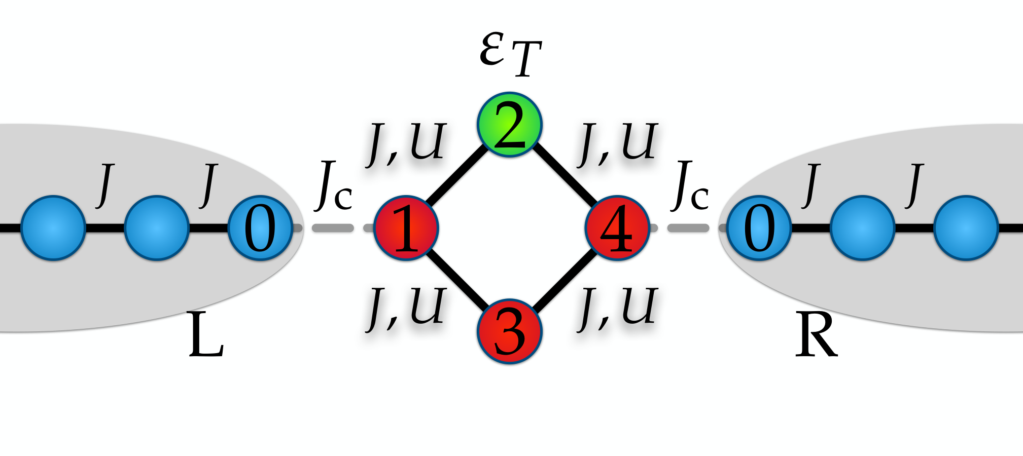

 (b)
(b)
 (b)
(b)

