Quasioptical modeling of wave beams with and without mode conversion:
III. Numerical simulations of mode-converting beams

Here, we outline how the general theory developed in Paper I can be applied, with some adjustments, to describe mode-converting wave beams. The general idea is similar to that presented in Paper II for single-mode waves. We assume a general linear equation for the electric field $\boldsymbol{\rm E}$ of a wave,

$$\displaystyle\smash{\widehat{\boldsymbol{\rm D}}}\boldsymbol{\rm E}=0,$$

(1)

where $\smash{\widehat{\boldsymbol{\rm D}}}$ is a linear dispersion operator. We also assume that this field can be represented in the eikonal form,

$$\displaystyle\boldsymbol{\rm E}=\boldsymbol{\rm\psi}e^{i\theta},$$

(2)

where $\boldsymbol{\rm\psi}$ is a slow complex vector envelope and $\theta$ is a fast real “reference phase” to be prescribed. The wave is considered stationary, so it has a constant frequency $\omega$; then $\boldsymbol{\rm\psi}$ and $\theta$ are functions of the spatial coordinate $\boldsymbol{\rm x}$. Correspondingly, the envelope $\boldsymbol{\rm\psi}$ satisfies

$$\displaystyle\smash{\widehat{\boldsymbol{\rm\mathcal{D}}}}\boldsymbol{\rm\psi}=0,\quad\smash{\widehat{\boldsymbol{\rm\mathcal{D}}}}\doteq e^{-i\theta(\boldsymbol{\rm x})}\smash{\widehat{\boldsymbol{\rm D}}}e^{i\theta(\boldsymbol{\rm x})},$$

(3)

where $\smash{\widehat{\boldsymbol{\rm\mathcal{D}}}}$ serves as the “envelope dispersion operator” ($\doteq$ denotes definitions). We introduce $\boldsymbol{\rm k}\doteq\nabla\theta(\boldsymbol{\rm x})$ for the local wave vector, $\lambda\doteq 2\pi/k$ for the corresponding wavelength, $L_{\parallel}$ for the inhomogeneity scale of $\boldsymbol{\rm\psi}$ along the beam, and $L_{\perp}$ for the minimum scale of $\boldsymbol{\rm\psi}$ across the beam. The medium-inhomogeneity scale is assumed to be larger than or comparable with $L_{\parallel}$, and we adopt

$$\displaystyle\epsilon_{\parallel}\doteq\lambda/L_{\parallel},\quad\epsilon_{\perp}\doteq\lambda/L_{\perp},\quad\epsilon_{\parallel}\sim\epsilon_{\perp}^{2}\ll 1.$$

(4)

Then, Eq. (3) becomes

$$\displaystyle\boldsymbol{\rm\mathsf{D}}\boldsymbol{\rm\psi}+\smash{\widehat{\boldsymbol{\rm\mathcal{L}}}}_{\epsilon}\boldsymbol{\rm\psi}=0,$$

(5)

where $\boldsymbol{\rm\mathsf{D}}$ serves as the “effective dispersion tensor” found from $\smash{\widehat{\boldsymbol{\rm D}}}$ and the operator $\smash{\widehat{\boldsymbol{\rm\mathcal{L}}}}_{\epsilon}=O(\epsilon_{\perp})$ is specified in Paper I (also see below). We suppose the following ordering:

$$\displaystyle\boldsymbol{\rm\mathsf{D}}_{H}=O(1),\quad\boldsymbol{\rm\mathsf{D}}_{A}=O(\epsilon_{\parallel}),$$

(6)

where the indices $H$ and $A$ denote the Hermitian and anti-Hermitian parts of $\smash{\widehat{\boldsymbol{\rm D}}}$, respectively. Assuming that the spatial dispersion is weak, $\boldsymbol{\rm\mathsf{D}}$ can be replaced with the homogeneous-plasma dispersion tensor,

$$\displaystyle\boldsymbol{\rm D}(\boldsymbol{\rm x},\boldsymbol{\rm p})=\frac{c^{2}}{16\pi\omega^{2}}\,[\boldsymbol{\rm p}\boldsymbol{\rm p}-(\boldsymbol{\rm p}\cdot\boldsymbol{\rm p})\mathbb{1}]+\frac{1}{16\pi}\,\boldsymbol{\rm\varepsilon}(\boldsymbol{\rm x},\boldsymbol{\rm p}),$$

(7)

where $\mathbb{1}$ is a unit matrix and $\boldsymbol{\rm\varepsilon}$ is the homogeneous-plasma dielectric tensor book:stix; its dependence on $\omega$ is assumed but not emphasized, since $\omega$ is constant. (Here, $\boldsymbol{\rm p}$ denotes any given wave vector, as opposed to $\boldsymbol{\rm k}$, which is the specific wave vector determined by $\theta$; see above.) Note that Eq. (7) assumes the Euclidean metric. Although we shall also use curvilinear coordinates below, expressing $\boldsymbol{\rm D}$ in those coordinates will not be necessary as explained in Sec. VI D of Paper I.

With $\boldsymbol{\rm\mathsf{D}}\approx\boldsymbol{\rm D}$ and $\boldsymbol{\rm D}$ given by Eq. (7), Eq. (6) implies $\boldsymbol{\rm\varepsilon}_{A}=O(\epsilon_{\parallel})$. Hence, $\boldsymbol{\rm D}_{H}$ is the dominant part of $\boldsymbol{\rm D}$, and Eq. (5) yields

$$\displaystyle\boldsymbol{\rm D}_{H}\boldsymbol{\rm\psi}=O(\epsilon_{\perp}).$$

(8)

Since the Hermitian matrix $\boldsymbol{\rm D}_{H}=O(1)$ is the dominant part of $\boldsymbol{\rm D}$ and has enough eigenvectors $\boldsymbol{\rm\eta}_{s}$ to form a complete orthonormal basis, it is convenient to represent the envelope $\boldsymbol{\rm\psi}$ in this basis,

$$\displaystyle\boldsymbol{\rm\psi}=\boldsymbol{\rm\eta}_{s}a^{s},$$

(9)

where $a^{s}$ are the complex amplitudes. [Summation over repeating indices is assumed. For all functions derived from $\boldsymbol{\rm D}$, such as $\boldsymbol{\rm\eta}_{s}$, the notation convention $f\equiv f(\boldsymbol{\rm x})\equiv f(\boldsymbol{\rm x},\boldsymbol{\rm k}(\boldsymbol{\rm x}))$ will also be assumed by default.] Then,

$$\displaystyle\boldsymbol{\rm D}_{H}\boldsymbol{\rm\psi}=\boldsymbol{\rm\eta}_{s}\Lambda_{s}a^{s},\quad\boldsymbol{\rm D}_{H}\boldsymbol{\rm\eta}_{s}=\Lambda_{s}\boldsymbol{\rm\eta}_{s}{\color[rgb]{0,0,0},}$$

(10)

where $\Lambda_{s}$ are the corresponding eigenvalues. Due to Eq. (8) and the mutual orthogonality of all $\boldsymbol{\rm\eta}_{s}$, this means that $\Lambda_{s}a^{s}$ is small for every given $s$ individually; hence, either $a^{s}$ is small or $\Lambda_{s}$ is small. In the latter case, $\boldsymbol{\rm\eta}_{s}$ approximately satisfies the eigenmode equation, $\boldsymbol{\rm D}_{H}\boldsymbol{\rm\eta}_{s}=\Lambda_{s}\boldsymbol{\rm\eta}_{s}\approx 0$, so it can be viewed as the local polarization vector of a GO mode. Then, the corresponding $a^{s}$ can be understood as the local scalar amplitude of an actual GO mode, and $a^{s}=O(1)$ is allowed.

In this paper, we consider the situation when there are two modes, henceforth called O and X modes, whose eigenvalues $\Lambda_{\rm o}\approx\Lambda_{\rm x}$ are both small within the region of interest. (This assumption is specified in Sec. II.4. Also note that the single-mode case is discussed in Paper II.) In other words, the two modes are approximately in resonance with each other. Then,

$$\displaystyle\boldsymbol{\rm\psi}=\boldsymbol{\rm\eta}_{\rm o}a^{\rm o}+\boldsymbol{\rm\eta}_{\rm x}a^{\rm x}+\bar{\boldsymbol{\rm\eta}}\bar{a},$$

(11)

where $\boldsymbol{\rm\eta}_{\rm o}$ and $\boldsymbol{\rm\eta}_{\rm x}$ are the O- and X-mode polarization vectors, $\bar{\boldsymbol{\rm\eta}}$ is some third eigenvector of $\boldsymbol{\rm D}$ that is orthogonal to both of them, and

$$\displaystyle a^{\rm o}=O(1),\quad a^{\rm x}=O(1),\quad\bar{a}=O(\epsilon_{\perp}).$$

(12)

The small amplitude $\bar{a}$ can be easily calculated as a perturbation and is included in our theory foot:paper1 but does not need to be considered below explicitly. Instead, we introduce a two-dimensional amplitude vector

$$\displaystyle\boldsymbol{\rm a}=\left(\begin{array}[]{c}a^{\rm o}\\ a^{\rm x}\end{array}\right)$$

and the $3\times 2$ “polarization matrix” $\boldsymbol{\rm\Xi}$ that contains the vectors $\boldsymbol{\rm\eta}_{\rm o}$ and $\boldsymbol{\rm\eta}_{\rm x}$ as its columns,

$$\displaystyle\boldsymbol{\rm\Xi}=\left(\begin{array}[]{cc}\boldsymbol{\rm\eta}_{\rm o}&\boldsymbol{\rm\eta}_{\rm x}\end{array}\right).$$

Then, $\boldsymbol{\rm\psi}$ can be expressed as follows:

$$\displaystyle\boldsymbol{\rm\psi}=\boldsymbol{\rm\Xi}\boldsymbol{\rm a}+O(\epsilon_{\perp}).$$

(16)

We also introduce the dual basis vectors $\boldsymbol{\rm\eta}^{\rm o}$ and $\boldsymbol{\rm\eta}^{\rm x}$ and an auxiliary polarization matrix

$$\displaystyle\boldsymbol{\rm\Xi}^{+}=\left(\begin{array}[]{c}\boldsymbol{\rm\eta}^{{\rm o}*}\\ \boldsymbol{\rm\eta}^{{\rm x}*}\end{array}\right).$$

As seen easily, this matrix satisfies $\boldsymbol{\rm\Xi}^{+}\boldsymbol{\rm\Xi}=\mathbb{1}$, and

$$\displaystyle\boldsymbol{\rm\Lambda}\doteq\boldsymbol{\rm\Xi}^{+}\boldsymbol{\rm D}_{H}\boldsymbol{\rm\Xi}=\left(\begin{array}[]{cc}\Lambda_{\rm o}&0\\ 0&\Lambda_{\rm x}\end{array}\right).$$

Also, one can express the amplitude vector as

$$\displaystyle\boldsymbol{\rm a}=\boldsymbol{\rm\Xi}^{+}\boldsymbol{\rm\psi}$$

(21)

[here, there is no $O(\epsilon_{\perp})$ correction, unlike in Eq. (16)], whose squared length $|\boldsymbol{\rm a}|^{2}\equiv|a^{\rm o}|^{2}+|a^{\rm x}|^{2}$ satisfies

$$\displaystyle|\boldsymbol{\rm a}|^{2}\approx|\boldsymbol{\rm\psi}|^{2}\equiv|\psi^{x}|^{2}+|\psi^{y}|^{2}+|\psi^{z}|^{2}$$

(22)

up to $O(\epsilon_{\parallel})$. Since we consider the beam dynamics in coordinates that are close to Euclidean, it will be sufficient, within the accuracy of our model, to adopt foot:paper1

$$\displaystyle\boldsymbol{\rm\eta}^{\rm o}\approx\boldsymbol{\rm\eta}_{\rm o}\quad\boldsymbol{\rm\eta}^{\rm x}\approx\boldsymbol{\rm\eta}_{\rm x}.$$

(23)

Then, $\boldsymbol{\rm\Xi}^{+}$ is simply the Hermitian conjugate of $\boldsymbol{\rm\Xi}$.

We consider the wave evolution in curvilinear coordinates that are linked to a “reference ray” (RR), which is governed by

$$\displaystyle\frac{\mathrm{d}X^{\alpha}}{\mathrm{d}\zeta}=\frac{V^{\alpha}_{\star}}{V_{\star}},\quad\frac{\mathrm{d}K_{\alpha}}{\mathrm{d}\zeta}=-\frac{1}{V_{\star}}\,\frac{\partial H_{\star}}{\partial X^{\alpha}}.$$

(24)

Here, $\zeta$ is the path along the ray, $\boldsymbol{\rm X}$ and $\boldsymbol{\rm K}$ are the RR coordinate and wave vector,

$$\displaystyle V_{\star}^{\alpha}(\zeta)\doteq\frac{\partial H(\boldsymbol{\rm X},\boldsymbol{\rm K})}{\partial K_{\alpha}}$$

(25)

is the group velocity, $V_{\star}\doteq|\boldsymbol{\rm V}_{\star}|$, and the index $\star$ denotes that the corresponding quantity is evaluated on $(\boldsymbol{\rm X},\boldsymbol{\rm K})$. In particular, $H_{\star}\doteq H(\boldsymbol{\rm X},\boldsymbol{\rm K})$, and $H$ is defined as follows:

$$\displaystyle H(\boldsymbol{\rm x},\boldsymbol{\rm p})\doteq\frac{1}{2}\,[\Lambda_{\rm o}(\boldsymbol{\rm x},\boldsymbol{\rm p})+\Lambda_{\rm x}(\boldsymbol{\rm x},\boldsymbol{\rm p})].$$

(26)

We require $H_{\star}$ to be exactly zero initially, which is ensured by choosing an appropriate $\boldsymbol{\rm K}$; then, $H_{\star}$ remains zero at all $\zeta$, as seen from Eqs. (24).

The RR-based coordinates are introduced as $\tilde{x}\equiv\{\zeta,\tilde{\varrho}^{1},\tilde{\varrho}^{2}\}$, where $\tilde{\varrho}^{\sigma}$ are orthogonal coordinates transverse to the RR as specified in Paper II. (Here and further, the indices $\sigma$ and ${\bar{\sigma}}$ span from 1 to 2; other Greek indices span from 1 to 3.) The basis vectors $\tilde{\boldsymbol{\rm e}}_{\mu}$ of the new coordinates ($\mathrm{d}\boldsymbol{\rm x}=\tilde{\boldsymbol{\rm e}}_{\mu}\mathrm{d}\tilde{x}^{\mu}$) are defined such that

$$\displaystyle\tilde{\boldsymbol{\rm e}}_{\star\mu}\cdot\tilde{\boldsymbol{\rm e}}_{\star\nu}=\delta_{\mu\nu},\quad\left[\partial\tilde{\boldsymbol{\rm e}}_{\sigma}(\tilde{x})/\partial\tilde{\varrho}^{\bar{\sigma}}\right]_{\star}=0.$$

(27)

Then,

$$\displaystyle\boldsymbol{\rm x}\approx\boldsymbol{\rm X}(\zeta)+\left(\begin{array}[]{cc}\tilde{\boldsymbol{\rm e}}_{\star 1}&\tilde{\boldsymbol{\rm e}}_{\star 2}\end{array}\right)\left(\begin{array}[]{c}\tilde{\varrho}^{1}\\ \tilde{\varrho}^{2}\end{array}\right).$$

For the transformation matrices defined as

	$$\displaystyle\mathcal{X}^{\alpha}{}_{\mu}\doteq\frac{\partial x^{\alpha}}{\partial\tilde{x}^{\mu}}=(\tilde{\boldsymbol{\rm e}}_{\mu})^{\alpha},$$		(31)
	$$\displaystyle\tilde{\mathcal{X}}^{\mu}{}_{\alpha}\doteq\frac{\partial\tilde{x}^{\mu}}{\partial x^{\alpha}}=(\boldsymbol{\rm\mathcal{X}}^{-1})^{\mu}{}_{\alpha},$$		(32)

this leads to

	$$\displaystyle\mathcal{X}^{\alpha}{}_{\zeta}\approx\mathcal{X}^{\alpha}_{\star}{}_{\zeta}+[(\tilde{\boldsymbol{\rm e}}_{\star\sigma})^{\alpha}]^{\prime}\tilde{\varrho}^{\sigma},$$		(33)
	$$\displaystyle\mathcal{X}^{\alpha}{}_{\sigma}\approx\mathcal{X}^{\alpha}_{\star}{}_{\sigma},$$		(34)
	$$\displaystyle\mathcal{X}^{\alpha}_{\star}{}_{\mu}=(\tilde{\boldsymbol{\rm e}}_{\star\mu})^{\alpha}{\color[rgb]{0,0,0}.}$$		(35)

The specific choice of $\tilde{\boldsymbol{\rm e}}_{\star\mu}$ is described in Paper II.

We shall use tilde to denote the components of vectors and tensors measured in the RR-based coordinates $\tilde{x}$. These components can be mapped to those in the laboratory coordinates using the standard formulas foot:paper2. For example, for any vector or covector $\boldsymbol{\rm A}$, one has

$$\displaystyle A^{\alpha}=\mathcal{X}^{\alpha}{}_{\mu}\tilde{A}^{\mu},\quad A_{\alpha}=\tilde{A}_{\mu}\tilde{\mathcal{X}}^{\mu}{}_{\alpha}.$$

(36)

We also introduce first-order partial derivatives

$$\displaystyle f_{|\alpha}\doteq\frac{\partial f(\boldsymbol{\rm x},\boldsymbol{\rm k})}{\partial x^{\alpha}},\quad f^{|\alpha}\doteq\frac{\partial f(\boldsymbol{\rm x},\boldsymbol{\rm k})}{\partial k_{\alpha}},$$

(37)

and the second-order derivatives are denoted as follows:

$$\displaystyle f_{|\alpha\beta}\doteq\frac{\partial^{2}f(\boldsymbol{\rm x},\boldsymbol{\rm k})}{\partial x^{\alpha}\partial x^{\beta}},\kern 5.0ptf^{|\alpha\beta}\doteq\frac{\partial^{2}f(\boldsymbol{\rm x},\boldsymbol{\rm k})}{\partial k_{\alpha}\partial k_{\beta}},\kern 5.0ptf^{|\alpha}_{|\beta}\doteq\frac{\partial^{2}f(\boldsymbol{\rm x},\boldsymbol{\rm k})}{\partial k_{\alpha}\partial x^{\beta}}.$$

Accordingly, $\tilde{f}_{|\mu}\doteq\partial f(\boldsymbol{\rm x},\boldsymbol{\rm k})/\partial\tilde{x}^{\mu}$, and so on.

Let us split the matrix (II.2) into its scalar part $H$ and its traceless part $\boldsymbol{\rm M}$; this gives $\boldsymbol{\rm\Lambda}=H\mathbb{1}+\boldsymbol{\rm M}$. We assume $\boldsymbol{\rm M}(\boldsymbol{\rm x},\boldsymbol{\rm k}(\boldsymbol{\rm x}))\lesssim O(\epsilon_{\perp})$ and $\boldsymbol{\rm M}_{\star}\lesssim O(\epsilon_{\parallel})$; then,

$$\displaystyle\boldsymbol{\rm M}(\boldsymbol{\rm x},\boldsymbol{\rm k}(\boldsymbol{\rm x}))=\boldsymbol{\rm M}_{\star}+\tilde{\boldsymbol{\rm M}}_{\star|\sigma}\tilde{\varrho}^{\sigma}+\tilde{\boldsymbol{\rm M}}{}_{\star}^{|\mu}\tilde{\pi}_{\mu}+o(\epsilon_{\parallel}),$$

(38)

where $\tilde{\pi}_{\mu}\doteq\tilde{k}_{\mu}(\boldsymbol{\rm x})-\tilde{K}_{\mu}(\zeta)$ is given by $\tilde{\pi}_{\mu}=-\tilde{\varrho}^{\sigma}\tilde{H}_{\star|\sigma}\tilde{V}_{\star\mu}/V_{\star}^{2}$ foot:paper2. We can also rewrite this as

	$$\displaystyle\boldsymbol{\rm M}(\boldsymbol{\rm x},\boldsymbol{\rm k}(\boldsymbol{\rm x}))=\boldsymbol{\rm M}_{\star}+\boldsymbol{\rm M}_{\star|\alpha}\varrho^{\alpha}+\boldsymbol{\rm M}{}_{\star}^{|\beta}\pi_{\beta}+o(\epsilon_{\parallel}),$$		(39)
	$$\displaystyle\varrho^{\alpha}\doteq\mathcal{X}_{\star}^{\alpha}{}_{\sigma}\tilde{\varrho}^{\sigma},\quad\pi_{\beta}=-\varrho^{\alpha}H_{\star|\alpha}V_{\star\beta}/V_{\star}^{2}.$$		(40)

This leads to

	$$\displaystyle\boldsymbol{\rm\Lambda}(\boldsymbol{\rm x},\boldsymbol{\rm k}(\boldsymbol{\rm x}))\approx H\mathbb{1}+\boldsymbol{\rm M}_{\star}+\tilde{\boldsymbol{\rm\mathfrak{M}}}_{\star\sigma}\tilde{\varrho}^{\sigma},$$
	$$\displaystyle\tilde{\boldsymbol{\rm\mathfrak{M}}}_{\star\sigma}\doteq(\boldsymbol{\rm M}_{\star|\alpha}-\boldsymbol{\rm M}{}_{\star}^{|\beta}H_{\star|\alpha}V_{\star\beta}/V_{\star}^{2})\mathcal{X}_{\star}^{\alpha}{}_{\sigma}.$$		(41)

Let us also introduce the matrices $\boldsymbol{\rm u}^{\alpha}\doteq\boldsymbol{\rm M}^{|\alpha}\lesssim O(\epsilon_{\perp})$,

$$\displaystyle\tilde{\boldsymbol{\rm u}}^{\sigma}=\tilde{\mathcal{X}}^{\sigma}{}_{\alpha}\boldsymbol{\rm u}^{\alpha}\approx\tilde{\boldsymbol{\rm u}}^{\sigma}_{\star}=\tilde{\mathcal{X}}^{\sigma}_{\star}{}_{\alpha}\boldsymbol{\rm M}^{|\alpha}_{\star},$$

(42)

and a rescaled amplitude vector

$$\displaystyle\boldsymbol{\rm\phi}\doteq\sqrt{V_{\star}}\boldsymbol{\rm a}.$$

(43)

By combining the results of Papers I and II, one readily finds that $\boldsymbol{\rm\phi}$ is governed by the following parabolic partial differential equation, which is the main “quasioptical” equation used in PARADE:

	$\displaystyle V_{\star}\partial_{\zeta}\boldsymbol{\rm\phi}=$	$\displaystyle-(\tilde{\boldsymbol{\rm u}}^{\sigma}_{\star}+\tilde{\boldsymbol{\rm\vartheta}}_{\star}^{\sigma}{}_{{\bar{\sigma}}}\tilde{\varrho}^{{\bar{\sigma}}})\partial_{\sigma}\boldsymbol{\rm\phi}-\frac{\tilde{\boldsymbol{\rm\vartheta}}_{\star}^{\sigma}{}_{\sigma}}{2}\boldsymbol{\rm\phi}$
		$\displaystyle+\frac{i}{2}\,\tilde{\boldsymbol{\rm\Phi}}^{\sigma{\bar{\sigma}}}_{\star}\partial^{2}_{\sigma{\bar{\sigma}}}\boldsymbol{\rm\phi}+\boldsymbol{\rm\Gamma}\boldsymbol{\rm\phi}$
		$\displaystyle-i(\tilde{\boldsymbol{\rm\mathfrak{L}}}_{\star\sigma{\bar{\sigma}}}\tilde{\varrho}^{\sigma}\tilde{\varrho}^{{\bar{\sigma}}}+\tilde{\boldsymbol{\rm\mathfrak{M}}}_{\star\sigma}\tilde{\varrho}^{\sigma}+\boldsymbol{\rm M}_{\star}-\boldsymbol{\rm U}_{\star})\boldsymbol{\rm\phi}.$		(44)

Here, we introduced the notation

$$\displaystyle\partial_{\zeta}\equiv\frac{\partial}{\partial\zeta},\quad\partial_{\sigma}\equiv\frac{\partial}{\partial\varrho^{\sigma}},\quad\partial_{{\bar{\sigma}}}\equiv\frac{\partial}{\partial\varrho^{{\bar{\sigma}}}}$$

(45)

and the following coefficients:

	$$\displaystyle\tilde{\boldsymbol{\rm\Phi}}^{\sigma{\bar{\sigma}}}_{\star}=\tilde{\mathcal{X}}_{\star}^{\sigma}{}_{\alpha}\tilde{\mathcal{X}}_{\star}^{{\bar{\sigma}}}{}_{\beta}H_{\star}^{|\alpha\beta}\mathbb{1},$$
	$$\displaystyle\boldsymbol{\rm\Gamma}=\boldsymbol{\rm\Xi}^{+}_{\star}\boldsymbol{\rm D}_{A}(\boldsymbol{\rm X}+\boldsymbol{\rm\varrho},\boldsymbol{\rm K}+\boldsymbol{\rm\pi})\boldsymbol{\rm\Xi}_{\star},$$
	$$\displaystyle\boldsymbol{\rm U}_{\star}=(H_{\star|\alpha}\boldsymbol{\rm\Xi}_{\star}^{+}\boldsymbol{\rm\Xi}_{\star}^{|\alpha}-H_{\star}^{|\alpha}\boldsymbol{\rm\Xi}_{\star}^{+}\boldsymbol{\rm\Xi}_{\star|\alpha}+\boldsymbol{\rm\Xi}_{\star}^{+|\alpha}\boldsymbol{\rm D}_{H}\boldsymbol{\rm\Xi}_{\star|\alpha})_{A}.$$

(As a reminder, the index $A$ in the latter formula denotes the anti-Hermitian part.) Also,

$$\tilde{\boldsymbol{\rm\vartheta}}_{\star}^{\sigma}{}_{{\bar{\sigma}}}=[H^{|\alpha}_{\star|\beta}-(V_{\star\gamma}/V^{2}_{\star})\,H^{|\alpha\gamma}_{\star}H_{\star|\beta}]\tilde{\mathcal{X}}^{\sigma}_{\star}{}_{\alpha}\mathcal{X}^{\beta}_{\star}{}_{{\bar{\sigma}}}\mathbb{1}\\ -(\tilde{\boldsymbol{\rm\mathcal{X}}}_{\star}\boldsymbol{\rm\mathcal{Y}}_{\star{\bar{\sigma}}}\tilde{\boldsymbol{\rm\mathcal{X}}}_{\star}\boldsymbol{\rm V}_{\star})^{\sigma},$$

(46)

the matrix $\tilde{\boldsymbol{\rm\vartheta}}_{\star}^{\sigma}{}_{\sigma}$ is obtained from here by setting ${\bar{\sigma}}=\sigma$ and summing over $\sigma$ accordingly, and

$$\displaystyle\boldsymbol{\rm\mathcal{Y}}_{\star\sigma}=\left(\begin{array}[]{ccc}[(\tilde{\boldsymbol{\rm e}}_{\star\sigma})^{1}]^{\prime}&0&0\\[3.0pt] [(\tilde{\boldsymbol{\rm e}}_{\star\sigma})^{2}]^{\prime}&0&0\\[3.0pt] [(\tilde{\boldsymbol{\rm e}}_{\star\sigma})^{3}]^{\prime}&0&0\end{array}\right).$$

Finally,

$$\tilde{\boldsymbol{\rm\mathfrak{L}}}_{\star\sigma{\bar{\sigma}}}=\frac{1}{2}\bigg(H_{\star|\alpha\beta}-\frac{2V_{\star\gamma}}{V^{2}_{\star}}\,H_{\star|\alpha}^{|\gamma}H_{\star|\beta}\\ +\frac{V_{\star\gamma}V_{\star\delta}}{V^{4}_{\star}}\,H^{|\gamma\delta}_{\star}H_{\star|\alpha}H_{\star|\beta}\bigg)\mathcal{X}_{\star}^{\alpha}{}_{\sigma}\mathcal{X}_{\star}^{\beta}{}_{{\bar{\sigma}}}\mathbb{1}.$$

(50)

Note that the structure of the two-mode quasioptical equation (44) is the same as that of the single-mode equation in Paper II except for the following: (i) there are additional terms $\tilde{\boldsymbol{\rm u}}_{\star}$, $\smash{\tilde{\boldsymbol{\rm\mathfrak{M}}}_{\star}}$, and $\boldsymbol{\rm M}_{\star}$; and (ii) the coefficients are matrices rather than scalars. In particular, $\boldsymbol{\rm U}$ and $\boldsymbol{\rm\Gamma}$ are generally non-diagonal and thus can cause mode conversion. Also note that, like in Paper II, one finds the following corollary:

$$\displaystyle\frac{\mathrm{d}P}{\mathrm{d}\zeta}=2\int(\boldsymbol{\rm a}^{\dagger}\boldsymbol{\rm\Gamma}\boldsymbol{\rm a})\,d^{2}\tilde{\varrho},$$

(51)

where $P\doteq\int|\boldsymbol{\rm\phi}|^{2}\,d^{2}\tilde{\varrho}$ equals, up to a constant coefficient, the energy flux carried by the beam. This shows that the total energy flux of the beam is conserved when $\boldsymbol{\rm\Gamma}=0$.

To facilitate benchmarking of PARADE, we also introduce the electromagnetic-field parametrization in terms of the polarization angles book:born65 used in the 1DFW code presented in . The two components of the field envelope $\boldsymbol{\rm\psi}$ projected on the transverse space $\{\tilde{\varrho}^{1},\tilde{\varrho}^{2}\}$ can be expressed as follows:

$$\displaystyle\left(\begin{array}[]{c}\tilde{\psi}^{1}_{\star}\\ \tilde{\psi}^{2}_{\star}\end{array}\right)=|\boldsymbol{\rm\psi}_{\star}|\left(\begin{array}[]{c}\cos\alpha\cos\beta-i\sin\alpha\sin\beta\\ \sin\alpha\cos\beta+i\cos\alpha\sin\beta\end{array}\right).$$

The geometrical meaning of the polarization angles $\alpha$ and $\beta$ can be understood from Fig. 1. Explicitly, these angles can be expressed through $\boldsymbol{\rm\psi}$ as book:born65

	$$\displaystyle\alpha=\frac{1}{2}\tan^{-1}\bigg(\frac{2|\tilde{\psi}^{1}_{\star}||\tilde{\psi}^{2}_{\star}|}{|\tilde{\psi}^{1}_{\star}|^{2}-|\tilde{\psi}^{2}_{\star}|^{2}}\cos\delta\bigg),$$		(56)
	$$\displaystyle\beta=\frac{1}{2}\sin^{-1}\bigg(\frac{2|\tilde{\psi}^{1}_{\star}||\tilde{\psi}^{2}_{\star}|}{|\tilde{\psi}^{1}_{\star}|^{2}+|\tilde{\psi}^{2}_{\star}|^{2}}\sin\delta\bigg)$$		(57)

(note the difference in the signs in the denominators), where $\delta\doteq\arg(\tilde{\psi}^{2}_{\star})-\arg(\tilde{\psi}^{1}_{\star})$. In the following PARADE simulations, the initial $\boldsymbol{\rm a}$ is prescribed by prescribing $\alpha$ and $\beta$. Specifically, $\alpha$ and $\beta$ determine $\tilde{\psi}^{\mu}$ via Eq. (II.5), and Eq. (21) yields $a^{s}=\eta^{s*}{}_{\alpha}\mathcal{X}^{\alpha}{}_{\mu}\tilde{\psi}^{\mu}$.

PARADE is also advantageous in that it can efficiently model splitting of multi-mode beams. To demonstrate this capability, we performed numerical simulations in a slab geometry with

	$$\displaystyle n=n_{0}\exp\bigg[-\frac{(x-x_{0})^{2}}{L_{n}^{2}}\bigg],$$		(66)
	$$\displaystyle\boldsymbol{\rm B}=\boldsymbol{\rm e}_{z}B_{0}\exp\bigg[-\frac{(x-x_{0})^{2}}{L_{b}^{2}}\bigg].$$		(67)

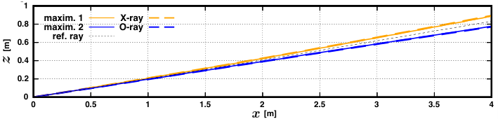
Here, $n_{0}=1.0\times 10^{19}$ m^-3, $x_{0}=4.0$ m, $L_{n}=4.0$ m, $B_{0}=1.0$ T, $L_{b}=4.0$ m, and $\boldsymbol{\rm e}_{z}$ is the unit vector along the $z$ axis. (The orientation of the magnetic field $\boldsymbol{\rm B}/|\boldsymbol{\rm B}|$ is chosen to be constant here to suppress the shear-driven mode conversion.) The origin is chosen to be the RR starting point, and $\{x,y,z\}=\{1.0,0.0,0.2\}$ m is chosen to be the target point, which is used to fix the orientation of the RR initial wave vector. The initial polarization angles are $\alpha=10.0^{\circ}$ and $\beta=-30.0^{\circ}$. Also, for the initial beam profile, we adopt a Gaussian profile foot:paper2; book:yariv with the focal lengths $\mathcal{Z}_{1}=\mathcal{Z}_{2}=3.0$ m and waist sizes $w_{0,1}=w_{0,2}=5.0$ cm. The wave frequency is chosen to be $f=77.0$ GHz. Figure 6 shows the evolution of the transverse profile of $|\boldsymbol{\rm a}|$ at different locations along the RR. One can see the gradual splitting of the original beam into O-mode and X-mode beams propagating along separate ray trajectories. (Note that a single RR is used for this simulation, in contrast to single-mode simulations, where each mode would have its own RR.) Figure 7 shows the trajectories of the locations of the amplitude maxima. For comparison, this figure also shows the trajectories obtained from ray-tracing simulations, where O and X waves are modeled as independent. It is seen that PARADE’s quasioptical simulations are in good agreement with conventional ray tracing. Importantly, such quasioptical modeling of a two-mode beam is adequate only as long as the group velocities of the O and X waves remain close enough to each other; otherwise the ordering (4) cannot be maintained. (That is why we consider only weak splitting here.) However, by the time the two group velocities become very different, the O and X waves also become nonresonant and thus independent. Such waves can also be modeled with PARADE, except the single-mode algorithm foot:paper2 must be used instead.

References

- (1) T. I. Tsujimura, S. Kubo, H. Takahashi, R. Makino, R. Seki, Y. Yoshimura, H. Igami, T. Shimozuma, K. Ida, C. Suzuki, M. Emoto, M. Yokoyama, T. Kobayashi, C. Moon, K. Nagaoka, M. Osakabe, S. Kobayashi, S. Ito, Y. Mizuno, K. Okada, A. Ejiri, T. Mutoh, and the LHD Experiment Group, Development and application of a ray-tracing code integrating with 3D equilibrium mapping in LHD ECH experiments, Nucl. Fusion 55, 123019 (2015).
- (2) N. B. Marushchenko, Y. Turkin, and H. Maassberg, Ray-tracing code TRAVIS for ECR heating, EC current drive and ECE diagnostic, Comput. Phys. Commun. 185, 165 (2014).
- (3) E. Mazzucato, Propagation of a Gaussian beam in a nonhomogeneous plasma, Phys. Fluids B 1, 1855 (1989).
- (4) S. Nowak and A. Orefice, Quasioptical treatment of electromagnetic Gaussian beams in inhomogeneous and anisotropic plasmas, Phys. Fluids B 5, 1945 (1993).
- (5) A. G. Peeters, Extension of the ray equations of geometric optics to include diffraction effects, Phys. Plasmas 3, 4386 (1996).
- (6) D. Farina, A quasi-optical beam-tracing code for electron cyclotron absorption and current drive: GRAY, Fusion Sci. Tech. 52, 154 (2007).
- (7) G. V. Pereverzev, Beam tracing in inhomogeneous anisotropic plasmas, Phys. Plasmas 5, 3529 (1998).
- (8) E. Poli, G. V. Pereverzev, A. G. Peeters, and M. Bornatici, EC beam tracing in fusion plasmas, Fusion Eng. Des. 53, 9 (2001).
- (9) E. Poli, A. G. Peeters, and G. V. Pereverzev, TORBEAM, a beam tracing code for electron-cyclotron waves in tokamak plasmas, Comput. Phys. Commun. 136, 90 (2001).
- (10) E. Poli, A. Bock, M. Lochbrunner, O. Maj, M. Reich, A. Snicker, A. Stegmeir, F. Volpe, N. Bertelli, R. Bilato, G. D. Conway, D. Farina, F. Felici, L. Figini, R. Fischer, C. Galperti, T. Happel, Y. R. Lin-Liu, N. B. Marushchenko, U. Mszanowski, F. M. Poli, J. Stober, E. Westerhof, R. Zille, A. G. Peeters, and G. V. Pereverzev, TORBEAM 2.0, a paraxial beam tracing code for electron-cyclotron beams in fusion plasmas for extended physics applications, Comput. Phys. Commun. 225, 36 (2018).
- (11) A. A. Balakin, M. A. Balakina, and E. Westerhof, ECRH power deposition from a quasi-optical point of view, Nucl. Fusion 48, 065003 (2008).
- (12) A. A. Balakin, M. A. Balakina, G. V. Permitin, and A. I. Smirnov, Quasi-optical description of wave beams in smoothly inhomogeneous anisotropic media, J. Phys. D: Appl. Phys. 40, 4285 (2007).
- (13) A. A. Balakin, M. A. Balakina, G. V. Permitin, and A. I. Smirnov, Scalar equation for wave beams in a magnetized plasma, Plasma Phys. Rep. 33, 302 (2007).
- (14) S. Kubo, H. Igami, T. I. Tsujimura, T. Shimozuma, H. Takahashi, Y. Yoshimura, M. Nishiura, R. Makino, and T. Mutoh, Plasma interface of the EC waves to the LHD peripheral region, AIP Conf. Proc. 1689, 090006 (2015).
- (15) I. Y. Dodin, D. E. Ruiz, and S. Kubo, Mode conversion in cold low-density plasma with a sheared magnetic field, Phys. Plasmas 24, 122116 (2017).
- (16) D. E. Ruiz, Geometric theory of waves and its applications to plasma physics, Ph.D. Thesis, Princeton Univ. (2017), arXiv:1708.05423.
- (17) D. E. Ruiz and I. Y. Dodin, Extending geometrical optics: A Lagrangian theory for vector waves, Phys. Plasmas 24, 055704 (2017).
- (18) D. E. Ruiz and I. Y. Dodin, Lagrangian geometrical optics of nonadiabatic vector waves and spin particles, Phys. Lett. A 379, 2337 (2015).
- (19) D. E. Ruiz and I. Y. Dodin, First-principles variational formulation of polarization effects in geometrical optics, Phys. Rev. A 92, 043805 (2015).
- (20) I. Y. Dodin, D. E. Ruiz, K. Yanagihara, Y. Zhou, and S. Kubo, Quasioptical modeling of wave beams with and without mode conversion: I. Basic theory, arXiv:1901.00268.
- (21) K. Yanagihara, I. Y. Dodin, and S. Kubo, Quasioptical modeling of wave beams with and without mode conversion: II. Numerical simulations of single-mode beams, submitted in parallel.
- (22) K. Y. Bliokh, F. J. Rodríguez-Fortuño, F. Nori, and A. V. Zayats, Spin-orbit interactions of light, Nat. Photonics 9, 796 (2015).
- (23) M. A. Oancea, C. F. Paganini, J. Joudioux, and L. Andersson, An overview of the gravitational spin Hall effect, arXiv:1904.09963.
- (24) K. Yanagihara, S. Kubo, T. I. Tsujimura, and I. Y. Dodin, Mode purity of electron cyclotron waves after their passage through the peripheral plasma in the Large Helical Device, to appear in Plasma Fusion Res..
- (25) T. H. Stix, Waves in Plasmas (AIP, New York, 1992).
- (26) M. Born and E. Wolf, Principles of Optics (Pergamon Press, Oxford, 1965).
- (27) A. Yariv, Quantum Electronics (Wiley, New Jersey, 1967).