Non-Hermitian dynamics without dissipation in quantum systems

A standard two-mode $\mathcal{PT}$ dimer consists of two tunnel-coupled modes (amplitudes $\alpha_{1}(t),\alpha_{2}(t)$) where mode $1$ ($2$) is subject to gain (loss), with the gain and loss rates set equal to $\gamma$ (see Fig. 1). The equations of motion are

where the $2\times 2$ effective non-Hermitian Hamiltonian is

$g$ is the tunneling amplitude (which we take without loss of generality to be real and positive), and $\sigma_{z},\sigma_{x}$ are standard Pauli matrices. We will use the calligraphic symbol $\mathcal{H}$ throughout to denote non-Hermitian Hamiltonians. Defining the time-reversal operation $\mathcal{T}$ as complex conjugation, and defining parity $\mathcal{P}$ as the interchange of the two modes, we see that ${\mathcal{H}_{\mathcal{PT}}}$ is invariant under $\mathcal{PT}$.

The eigenvalues of ${\mathcal{H}_{\mathcal{PT}}}$ are given by

At the critical point $g=\gamma/2\equiv g_{c}$, the $\mathcal{PT}$-symmetric Hamiltonian $\mathcal{H}_{\mathcal{PT}}$ is defective, corresponding to a (second order) exceptional point in parameter space. For $g<g_{c}$, the mode eigenvalues become complex, implying exponential growth and decay in the time domain; this transition is often referred to as the “spontaneous breaking of $\mathcal{PT}$ symmetry”.

Consider next a more general non-Hermitian 2 mode problem, where the dynamics are again given by Eq. (1) with $\mathcal{H}_{\mathcal{PT}}$ replaced by a more general effective Hamiltonian:

Here ${\vec{c}}$, $\vec{d}$ are real vectors, and we have ignored any constant-matrix part of $\mathcal{H}$ (as this has a trivial effect on dynamics). This general non-Hermitian Hamiltonian is unitarily equivalent to $\mathcal{H}_{\mathcal{PT}}$ (and has eigenvalues of the form in Eq. (3)) whenever its Hermitian and anti-Hermitian parts are orthogonal, i.e.

While the preceding discussion is all classical, one might think that the extension to a quantum setting is trivial: just replace mode amplitudes $\alpha_{1}(t),\alpha_{2}(t)$ in Eq. (1) by canonical bosonic Heisenberg-picture annihilation operators $\hat{a}_{1}(t),\hat{a}_{2}(t)$, and interpret the result as a set of coupled Heisenberg equations of motion. This in general is not a valid evolution, as the dynamics will not preserve canonical commutation relations, i.e. at all times $[\hat{a}_{j}(t),\hat{a}^{\dagger}_{j^{\prime}}(t)]=\delta_{jj^{\prime}}$. This is perhaps most evident in the simple case where $g=0$, and one has simple exponential growth (decay) of mode 1 (2).

At a physical level, this inconsistency arises because the gain/loss terms that give rise to the non-Hermitian part of $\mathcal{H}$ arise from couplings to dissipative environments. In addition to providing gain/loss, these baths will also drive the system with noise, and this noise cannot be neglected in the quantum case. By adding appropriate inhomogeneous quantum noise terms to the RHS of Eq. (1), one can then obtain an allowed quantum evolution (i.e. commutation relations are preserved in time). A systematic procedure for constructing quantum noise terms consistent with a given non-Hermitian Hamiltonian was presented recently in Ref. HKLau2018.

Our goal is to realize the effective non-Hermitian dynamics of Eq. (1) in a quantum system without having dissipation and the corresponding driving noise. To that end, we consider the quantum Hamiltonian of a single bosonic mode $\hat{a}$ that is parametrically driven (i.e. subject to two-photon driving). In an appropriate rotating frame, the Hamiltonian is:

where $\delta$ represents a detuning term, and $\nu$ is the magnitude of the parametric drive. This is the basic Hamiltonian of a degenerate parametric amplifier (DPA). Without loss of generality, we work in a gauge where $\nu$ is real and positive in what follows.

Despite having only a single mode, the dynamics has a 2 component structure, as the parametric drive couples $\hat{a}$ and $\hat{a}^{\dagger}$. Defining a vector of operators

the Heisenberg equations of motions can be written as

where the dynamical matrix $\mathcal{M}_{\mathrm{DPA}}$ is

We see immediately that the structure of the Heisenberg EOM for this Hermitian problem mirrors that of the effective non-Hermitian dimer system in Eq. (1), with the dynamical matrix $\mathcal{M}_{\mathrm{DPA}}$ playing the role of an effective non-Hermitian Hamiltonian $\mathcal{H}$. Further, $\mathcal{M}_{\mathrm{DPA}}$ satisfies the condition in Eq. (4), implying that it is unitarily equivalent to $\mathcal{H}_{\mathcal{PT}}$ in Eq. (2) (with $\delta=g$ and $\nu=\gamma/2$). This effective $\mathcal{PT}$ symmetry cannot be broken in our single mode problem (as Eq. (6) is the most general single-mode, quadratic, Hermitian and bosonic Hamiltonian).

Not surprisingly, the eigenvalues of $\mathcal{M}_{\mathrm{DPA}}$ have exactly the same structure as the $\mathcal{PT}$ dimer:

It follows that the parametric drive $\nu$ plays the role of the incoherent gain/loss in $\mathcal{H}_{\mathcal{PT}}$, whereas the detuning $\delta$ plays the role of the tunnel coupling. As we show in the next subsection, this allows us to directly map the physics of the threshold transition in our DPA system to the “spontaneous” breaking of $\mathcal{PT}$-symmetry that occurs in $\mathcal{H}_{\mathcal{PT}}$ when $\gamma/2$ is made larger than $g$. In particular, the DPA dynamical matrix exhibits an exceptional point when $\nu=\delta$, i.e. at the parametric oscillation threshold.

Before exploring this connection, we return to the problem of commutation relations: why doesn’t the non-Hermitian nature of the dynamical matrix (and the possibility of exponential growth / decay) in time cause issues in our DPA system? The easiest way of seeing this is to explicitly make the unitary transformation that maps the dynamical matrix $\mathcal{M}_{\mathrm{DPA}}$ in Eq. (9) to the gain-loss form of $\mathcal{H}_{\mathcal{PT}}$ in Eq. (2). With this transformation, the Heisenberg equations of motion in Eq. (8) now take the form:

where $\hat{q}\equiv(\hat{a}+\hat{a}^{\dagger})/\sqrt{2}$, $\hat{p}\equiv i(\hat{a}^{\dagger}-\hat{a})/\sqrt{2}$ are canonical (Hermitian) quadrature operators. With this transformation, we see that the dynamical matrix for the DPA in the quadrature basis has explicitly the same form as the non-Hermitian Hamiltonian $\mathcal{H}_{\mathcal{PT}}$ in Eq. (2) describing the gain-loss $\mathcal{PT}$ dimer. We can also see why there is no longer any issue with commutation relations: the exponential growth that occurs when $|\delta|<\nu$ causes $\hat{q}$ to grow exponentially in time, and $\hat{p}$ to decay exponential in time, at the same rate. This is just standard, unitary squeezing dynamics. This exponential growth preserves the canonical $[\hat{q},\hat{p}]=i$ commutation relation at all times.

We thus see that by exploiting the squeezing / anti-squeezing, we can replicate the dynamics of the non-Hermitian $\mathcal{PT}$ dimer in Eq. (1). Of course, in this mapping we have just a single mode, and hence only a single complex degree of freedom (whereas in Eq. (1), there are two complex degrees of freedom). In Eq. (11), this manifests itself in the fact that the relative phase between the two amplitudes must be $i$. By using a two-mode, non-degenerate parametric amplifier system, this phase constraint can be lifted; this will be discussed in Sec. III.1. Sec. II.4 presents yet another approach allowing even more flexibility.

Before proceeding, we briefly pause to note another connection between the $\mathcal{PT}$ dimer Hamiltonian $\mathcal{H}_{\mathcal{PT}}$ and the DPA dynamical matrix $\mathcal{M}_{\mathrm{DPA}}$: they are are both pseudo-Hermitian matrices. By definition, a pseudo-Hermitian matrix is isospectral with its Hermitian conjugate, so that

where $\eta$ is Hermitian and invertible JMP20021. It is easy to see that the dynamical matrix of a generic multi-mode bosonic parametric amplifier system is pseudo-Hermitian; this was recently explicitly pointed out by Lieu Lieu2018 (see also Appendix A). This connection is however of limited use for our problem: while a given $\mathcal{PT}$-symmetric Hamiltonian is always pseudo-Hermitian, it is not necessarily unitarily equivalent to the dynamical matrix of some quantum bosonic system having the same number of modes (see Appendix E).

A consequence of the above mapping is that the so-called $\mathcal{PT}$ symmetry breaking phase transition in $\mathcal{H}_{\mathcal{PT}}$ is equivalent to the threshold transition in a parametric amplifier. Recall that $\mathcal{H}_{\mathcal{PT}}$ exhibits a transition in the eigenvectors and eigenvalues as a function of $g$; this is referred to as the “spontaneous breaking of $\mathcal{PT}$ symmetry” Bender2013. The transition occurs at $g=\gamma/2\equiv g_{c}$, i.e. the point at which $\mathcal{H}_{\mathcal{PT}}$ has an exceptional point. When $g>g_{c}$, one is in the $\mathcal{PT}$-unbroken phase. $\mathcal{H}_{\mathcal{PT}}$ has purely real eigenvalues, and its right eigenvectors ${{\vec{r}}_{\pm}}$ are delocalized (i.e. their amplitudes in each mode are equal) as

with $\alpha=\arccos\left({\gamma/2g}\right)$. In contrast, when $g$ is reduced below $g_{c}$, one is in the $\mathcal{PT}$-broken phase. $\mathcal{H}_{\mathcal{PT}}$ has purely imaginary eigenvalues, and the eigenvectors now exhibit localization.

The above behaviour is equivalent to the threshold behaviour of a detuned DPA. For $|\delta|>\nu$, the parametric drive is too non-resonant to cause any instability, and the system has purely oscillatory dynamics (as it would if $\nu=0$). In contrast, when $|\delta|$ is reduced below $\nu$, one crosses the threshold for parametric instability. One now has exponential decay and growth, which (as discussed) corresponds to the squeezing / anti-squeezing of canonically conjugate quadratures. The effective localization of the eigenvectors in this regime corresponds to the fact that the amplified quadrature is predominantly $\hat{q}$, while the squeezed quadrature is predominantly $\hat{p}$.

Finally, consider the case where one tunes $\delta=\nu$ and is thus exactly at the EP. The DPA Hamiltonian in this case is:

The Hermitian quadrature operator $\hat{Q}$ is a conserved quantity, and thus $\hat{H}_{\rm DPA}$ is said to possess a quantum non-demolition (QND) structure. This structure is directly responsible for the lack of any oscillatory dynamics. The co-existence of exceptional points and conserved QND quadrature operators is not just limited to this simple example: it is a generic feature in particle non-conserving bosonic Hamiltonians. For example, in Appendix F, we discuss a 3-mode system that can be tuned to a third-order EP; this coincides with it having two conserved QND quadrature operators.

We now discuss a more general approach for realizing non-Hermitian two-mode dynamics in dissipation-free quantum systems. Unlike the mapping to a DPA discussed in Sec. II.2, this alternate method does not require a $\mathcal{PT}$-symmetric non-Hermitian Hamiltonian $\mathcal{H}$, and does not place restrictions on the phases of mode amplitudes. Our approach adapts the concept of quantum-mechanics free subsystems (QMFS) introduced by Tsang and Caves Caves2012: by introducing extra bosonic modes, one can have a commuting set of operators with arbitrary (possibly non-Hermitian) dynamics. As all relevant operators commute, there is no need to add noise terms. While QMFS are conventionally discussed and utilized for quantum back-action evasion Caves2012; Clerk2013; Clerk2015; Polzik2017; Polzik2018, we show here that they are also a powerful tool for realizing effective non-Hermitian quantum dynamics in a dissipationless setting.

Consider a two-mode non-Hermitian system where $\mathcal{PT}$ is explicitly broken by the addition of a detuning term $\omega$:

This Hamiltonian is not unitarily equivalent to a $\mathcal{PT}$ system (c.f. Eq. (5)), and thus its dynamics cannot be realized by a DPA using the mapping of Sec. II.2.

As usual, the goal is to have a quantum system whose Heisenberg equations of motion are governed by $\mathcal{H}_{\omega}$ without any extra added quantum noise terms, i.e.

The operators $\hat{z}_{j}$ should play the analogous role of the mode amplitudes in the classical coupled-mode equations Eq. (2), and hence should encode two complex degrees of freedom. As discussed, the obvious choice where $\hat{z}_{j}$ represent canonical annihilation operators of two bosonic modes does not work: the resulting dynamics would not in general preserve canonical commutation relations.

Clearly, a simple solution would be to use operators $\hat{z}_{j}$ where for all $j,j^{\prime}$

As all operators commute, there would be no additional quantum constraints on Eq. (16). Throughout this paper, we will use the term pseudo-modes to denote a set of fully commuting operators $\hat{z}_{j},\hat{z}^{\dagger}_{j}$ that obey some desired non-Hermitian dynamics. While these pseudo-mode operators are not canonical bosonic annihilation / creation operators, they can play the role of mode amplitudes in the classical coupled mode theory.

For our two-mode problem, we can construct appropriate pseudo-modes by considering a system of four canonical bosonic modes, with annihilation operators $\hat{a}_{1},\hat{a}_{2},\hat{b}_{1},\hat{b}_{2}$. Each mode can be written in terms of Hermitian quadrature operators ($j=1,2$):

One could now also define collective quadrature operators in the standard manner:

These satisfy standard canonical commutation relations, namely $\left[{{{\hat{x}}_{\pm,j}},{{\hat{p}}_{\pm,j^{\prime}}}}\right]=i{{\delta}_{jj^{\prime}}}$, $\left[{{{\hat{x}}_{\pm,j}},{{\hat{x}}_{\mp,j^{\prime}}}}\right]=\left[{{{\hat{p}}_{\pm,j}},{{\hat{p}}_{\mp,j^{\prime}}}}\right]=\left[{{{\hat{x}}_{\pm,j}},{{\hat{p}}_{\mp,j^{\prime}}}}\right]=0$. Note that all $+$ collective quadrature operators commute with all $-$ operators.

We can now construct non-Hermitian pseudo-mode operators $\hat{z}_{j}$ with the desired properties by building them out of a fully commuting set of four collective quadrature operators. While there are many possible choices, we will use:

Eq. (17) is thus satisfied: we have two complex degrees of freedom where there are no constraints from commutation relations.

All that remains is to construct a physical (Hermitian) Hamiltonian where the four collective quadratures of interest are dynamically coupled as per Eq. (16). This can be accomplished using

This represents a system of two tunnel-coupled non-degenerate parametric amplifiers. One can verify that the Heisenberg equations of motion for collective quadratures generated by the Hermitian Hamiltonian ${{\hat{H}}_{\omega\mathrm{PA}}}$ correspond to Eq. (16), with the pseudo-modes defined in Eq. (21). We thus have our desired mapping.

Note that with this choice, the collective quadratures that do not appear in the definition of $\hat{z}_{j}$ can be used to construct another pair of pseudo-modes:

The dynamics does not couple $\hat{z}$ and $\hat{\tilde{z}}$ operators; using Eq. (22), the latter satisfy:

Thus, in doubling the degrees of freedom, we have constructed two sets of commuting “pseudo-mode” operators; the first set evolves according to $\mathcal{H}_{\omega}$, the second to $\mathcal{H}^{\dagger}_{\omega}$.

It is instructive to also consider the structure of the Heisenberg equations of motion when written in terms of the true canonical mode annihilation operators; the desired non-Hermitian structure is present there as well. Letting $\left|{\hat{v}}_{2}\right\rangle$ denote the four-vector of operators ${({{\hat{a}_{1}},{\hat{a}_{2}},{\hat{b}_{1}^{\dagger}},{\hat{b}_{2}^{\dagger}}})^{T}}$, the Heisenberg equations of motion generated by $\hat{H}_{\omega\mathrm{PA}}$ have the general form

Here ${{\mathcal{M}}_{\omega\mathrm{PA}}}$ is the system’s mode-basis dynamical matrix; it is unitarily equivalent to a $\mathcal{PT}$-symmetric matrix:

This provides another way to interpret our mapping: by doubling the degrees of freedom and introducing a mirror system of the detuned $\mathcal{PT}$ dimer $\mathcal{H}_{\omega}$ in Eq. (15) which evolves under $\mathcal{H}^{*}_{\omega}=\mathcal{H}^{\dagger}_{\omega}$, we effectively restore $\mathcal{PT}$ symmetry for the entire, composite system, allowing a mapping to a parametrically-driven bosonic Hamiltonian.

We end this section by stressing that our construction using four modes is not limited to the particular non-Hermitian Hamiltonian $\mathcal{H}_{\omega}$, but can be used to realize the dynamics of any non-Hermitian two-mode Hamiltonian $\mathcal{H}$. One again represents the quasi-mode operators $\hat{z}_{1}$ and $\hat{z}_{2}$ using Eqs. (21). One obtains the desired dynamics in Eq. (16) (with $\mathcal{H}_{\omega}$ replaced by $\mathcal{H}$) if the Hermitian Hamiltonian describing the four mode system is taken to be:

We see that the particle-number conserving terms are associated with the Hermitian part of $\mathcal{H}$, whereas the non-Hermitian parts of $\mathcal{H}$ are associated with particle-nonconserving two-photon driving terms.

We start with a simple, but paradigmatic case: a one-dimensional, nearest-neighbour tight-binding chain with on-site gain/loss terms that respects $\mathcal{PT}$ symmetry. We refer to this as a “standard” $\mathcal{PT}$ tight-binding chain. Non-Hermitian lattice models of this form have been the subject of many recent studies (see, e.g., Christodoulides2011; Wiersig2014; Yang2017; Szameit2017; Barnett2013; Lieu2018; Lieu2018a). We show that it is possible to realize identical dynamics in a Hermitian driven bosonic system, without any need to introduce dissipation or double the number of degrees of freedom. We also show that this approach can be generalized to a wider class of models.

We consider a 1D lattice of coupled modes having $2N$ sites, labelled (from left to right) by $j\in\{-N,-N+1,...,-1,1,...,N-1,N\}$. We will also (as is common) describe our non-Hermitian Hamiltonian using second-quantized notation, with $\hat{c}_{j}$ being the mode annihilation operator on site $j$. The non-Hermitian lattice Hamiltonian then has the form:

The first three terms represents Hermitian hopping on the lattice, with hopping strength $t_{j}$ on each bond (which we take to be real without loss of generality). The last, non-Hermitian term describes on-site gain/loss on each site, with a corresponding rate $\gamma_{j}/2$.

We now constrain this model by insisting that it be $\mathcal{PT}$-symmetric. $\mathcal{P}$ is defined as the real-space operation which maps $\hat{c}_{j}$ to $\hat{c}_{-j}$, and $\mathcal{T}$ is defined as before as simple complex conjugation of the Hamiltonian matrix. $\mathcal{PT}$ symmetry thus requires:

Note that the class of models of this form includes the widely-studied non-Hermitian $\mathcal{PT}$-symmetric Su-Schrieffer-Heeger (SSH) model SSH1979; Szameit2017; Barnett2013; OL2013. This would correspond to a dimerized structure for the hoppings and loss: ${t_{j}}=t+{\left(-\right)^{j}}t^{\prime}$ and ${\gamma_{j}}={\left(-\right)^{j}}{\gamma_{0}}$.

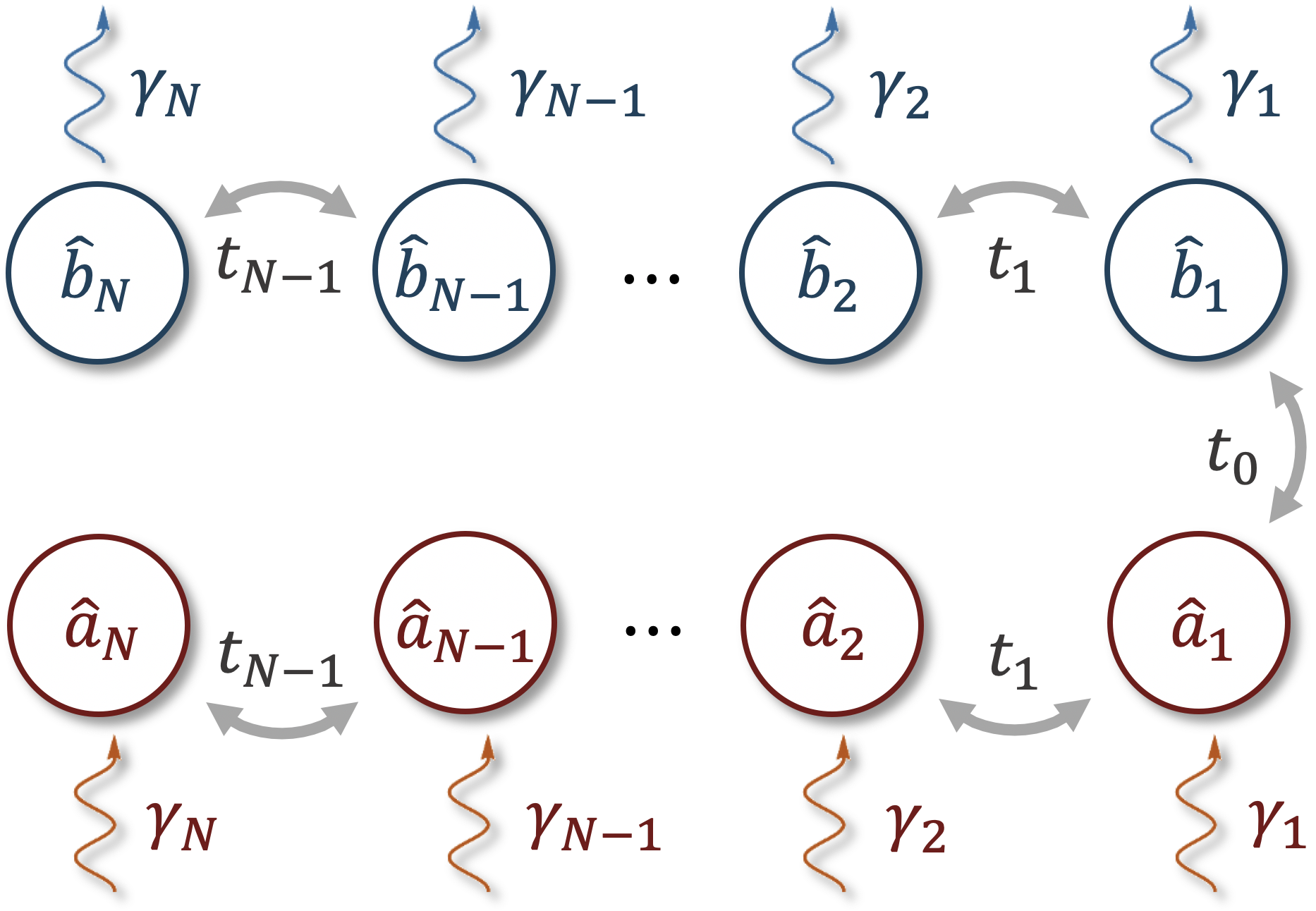
It will be useful to re-write the Hamiltonian in a more structured form by relabelling the mode operators via

As depicted in Fig. 2, the Hamiltonian becomes

where $\Omega,\Gamma,J$ and ${\tilde{J}}$ are all $N\times N$ coefficient matrices with entries given by

In this new basis, $\mathcal{P}$ is simply the operation which interchanges ${{a}_{j}}$ and ${{b}_{j}}$ ($j=1,2,\cdots,N$).

We now proceed in analogy to our treatment of the $\mathcal{PT}$ dimer in Sec. II.2. We first obtain the equations of motion for the ${{a}_{j}}$ and ${{b}_{j}}$ modes amplitudes ${{\alpha}_{j}}$ and ${{\beta}_{j}}$, generated by $\hat{\mathcal{H}}_{\rm tb}$ as

with the resulting non-Hermitian dynamical matrix given by

with ${\tilde{J}}=J$.

The block structure of the matrix $\mathcal{H}_{\mathrm{tb}}$ (corresponding to ${{a}_{j}}$/${{b}_{j}}$ modes) allows us to make a simple rotation ${\mathcal{U}_{\mathrm{tb}}}$ which moves the non-Hermitian gain/loss terms to the off-diagonal blocks:

In analogy to the two-mode problem in Sec. II.2, the rotated matrix ${\mathcal{M}_{\mathrm{tb}}}$ now has the form of a dynamical matrix of a parametrically driven bosonic system with $2N$ sites. However, unlike the mapping in Sec. II.2, the relevant system here involves non-degenerate parametric drives (i.e. two-photon driving terms that involve distinct modes). The dynamical matrix ${\mathcal{M}_{\mathrm{tb}}}$ above corresponds to the Hermitian bosonic Hamiltonian

To be explicit, the Heisenberg equations of motion corresponding to this Hermitian Hamiltonian can be compactly written as

where $\left|{\hat{v}}_{N}\right\rangle={({{\hat{a}_{1}},{\hat{a}_{2}},\cdots,{\hat{a}_{N}},{\hat{b}_{1}^{\dagger}},{\hat{b}_{2}^{\dagger}},\cdots,{\hat{b}_{N}^{\dagger}}})^{T}}$. Thus, we see that the dynamics of the general $\mathcal{PT}$-symmetric non-Hermitian gain-loss lattice model in Eq. (36) can be realized by the non-dissipative, Hermitian quantum Hamiltonian in Eq. (46). As before, the exponential growth and decay that could result from the gain and loss terms are mapped onto a unitary squeezing operations in the driven quantum model (in this case two-mode squeezing operations).

With this explicit non-degenerate parametric-amplifier (NDPA) Hamiltonian ${\hat{H}}_{\mathrm{NDPA}}$ in hand, it is interesting to return to the simple $\mathcal{PT}$ dimer discussed in Sec. II.2. This corresponds to the case $N=1$ of the 1D $\mathcal{PT}$ chain considered in this section. In this case, the matrix $\Omega$ becomes an overall constant in the non-Hermtian Hamiltonian $\hat{\mathcal{H}}_{\rm tb}$ and can be ignored, and our mapping shows that the dynamics is equivalent to a simple two-mode NDPA in Eq. (46). We stress that this is a distinct mapping from that in Sec. II.2, which involves a single-mode DPA. By having two modes here, there is no constraint on the phases of mode amplitudes, as the number of complex degrees of freedom is the same as the original non-Hermitian coupled-mode problem. As we will show in the next section, this lack of constraints remains the same in the general multi-mode version of the problem as well.

We now consider more general $\mathcal{PT}$-symmetric non-Hermitian lattice models, which could be in higher dimensions, have long range hopping terms, and have non-local non-Hermitian terms. The unitary mapping ${\mathcal{U}_{\mathrm{tb}}}$ derived above is also valid for a wide class of these generalized models. Note first that a generic $\mathcal{PT}$-symmetric non-Hermitian Hamiltonian (in arbitrary dimensions, with $2N$ sites) can always be written in the form given in Eq. (36), where $\mathcal{PT}$ symmetry requires that the coefficient matrices $\Omega,\Gamma$ are real, as well as $\tilde{J}=J^{*}$. Our mapping to a Hermitian parametric amplifier problem (as per Eq. (46)) remains valid as long as the coefficient matrices $\Omega$, $\Gamma$ and $J$ are all real, symmetric matrices. This encompasses a much broader class of models than the 1D nearest neighbour, imaginary potential model described by Eqs. (37).

Among the extra kinds of terms that can be accommodated in the starting non-Hermitian $\mathcal{PT}$ lattice model are:

• •

  real detunings of $a_{j}$ and $b_{j}$ modes, given by real, diagonal matrix elements of $\Omega$;

• •

  real, coherent (i.e. Hermitian) coupling between any two $a_{j}$ and $a_{j^{\prime}}$ (or $b_{j}$ and $b_{j^{\prime}}$) modes with a completely real coupling strength, represented by off-diagonal matrix elements of $\Omega$;

• •

  real, coherent coupling between any two $a_{j}$ and $b_{j^{\prime}}$ modes with a completely real coupling strength, represented by corresponding matrix elements of $J$;

• •

  imaginary, dissipative (i.e. non-Hermitian) couplings between any two different modes, represented by off-diagonal matrix elements of $\Gamma$.

As an example, our mapping to a NDPA system remains valid for a 2D tight-binding $\mathcal{PT}$ lattice, as long as the coherent couplings are purely real, and the dissipative couplings are purely imaginary. Conversely, for non-Hermitian tight-binding models where hopping phases encode non-trivial fluxes, we may construct an example where the mapping does not work. Necessary conditions for such a mapping to exist are presented in Appendix C, while simple four mode systems where the correspondence fails are discussed in Appendix E.

In Sec. III.1 and III.2, we described a general mapping between a wide class of non-Hermitian, $\mathcal{PT}$ symmetric lattice models and the dynamical matrix of a Hermitian, parametrically driven bosonic system. Crucially, this mapping preserved the number of modes. As discussed, it cannot be applied to all possible $\mathcal{PT}$ lattice models, nor can it be used for systems with broken $\mathcal{PT}$.

In this section, we show how the general QMFS strategy introduced in Sec. II.4 can be generalized to map an arbitrary non-Hermitian lattice model to a Hermitian, parametrically-driven bosonic problem. While more general, this strategy comes with a price: the driven bosonic system will have twice the number of modes as in the original non-Hermitian Hamiltonian.

The approach is to generalize the construction presented in Eq. (32) of Sec. II.4 to a general $N$-mode non-Hermitian Hamiltonian $\mathcal{H}_{N}$. We will use a $2N$-mode bosonic system, with canonical quadrature operators ${\hat{x}_{\pm,j}}$ and ${\hat{p}_{\pm,j}}$ for $j=1,2,\ldots,N$. The only nonzero commutators between the quadratures are

for $j,j^{\prime}=1,2,\ldots,N$.

To implement the general QMFS strategy, we wish to construct a Hamiltonian where a set of fully commuting collective quadratures has a linear dynamics corresponding to $\mathcal{H}_{N}$. Following the convention for the two-mode case in Eqs. (21,23), we first introduce two sets of pseudo-modes $\hat{{z}}_{\pm,j}~(j=1,2,\ldots,N)$ as

Mirroring the strategy of Sec. II.4, we want a Hermitian bosonic Hamiltonian that yields the equations of motion:

where we define $N$-vectors ${\vec{\hat{z}}}_{\pm}$ consisting of the pseudo-mode operators ${{\hat{z}}}_{\pm,j}$, respectively, for notational convenience. As before, the desired dynamics will only couple mutually commuting quadratures. It is straightforward to prove that the two equations above generate a dynamics that preserve all canonical commutation relations, i.e. they generate a symplectic transformation of the bosonic system (see Appendix G.2 for details). Further, one can show that this dynamics is generated by the Hermitian $2N$-mode Hamiltonian

where we define the bosonic mode operators in parallel to Eq. (21) as

The approach here is of course directly applicable to the case where the non-Hermitian $\mathcal{H}_{N}$ describes a lattice model in real space. Our mapping doubles the number of modes: for every lattice site in the original model, there are now two bosonic modes $\hat{a}_{j},\hat{b}_{j}$. Note however from Eq. (51) that our mapping is fully local. For every band $E_{n}(\vec{k})$ of $\mathcal{H}_{N}$, the closed-form dynamics of the ${\hat{a}}_{j}$ and ${\hat{b}_{j}^{\dagger}}$ operators will correspondingly contribute two independent bands $E_{n}(\vec{k})$ and $E_{n}^{*}(\vec{k})$ in the bosonic problem; this follows directly from Eqs. (50a)-(50b). We stress that this doubled band structure only solves half of the entire BdG problem of the bosonic Hamiltonian; the full band structure will also include contributions from dynamics of the ${\hat{b}}_{j}$ and ${\hat{a}_{j}^{\dagger}}$ operators, which can also be obtained from Eqs. (50a)-(50b) as the $-E_{n}(\vec{k})$ and $-E_{n}^{*}(\vec{k})$ bands.

We first consider sensing methods that exploit the strong sensitivity of mode eigenvalues of a $\mathcal{PT}$-symmetric non-Hermitian system that is tuned to the vicinity of an exceptional point (EP) Wiersig2014; Yang2017. The most common version of this scheme involves a simple gain-loss $\mathcal{PT}$ dimer (c.f. Sec. II.1) with an effective non-Hermitian Hamiltonian

The goal is to estimate the small parameter $\epsilon$. If the unperturbed Hamiltonian $\mathcal{H}\left[0\right]$ is tuned to the EP by choosing $g_{0}=\gamma/2=g_{c}$, then the perturbation $\epsilon$ induces an eigenvalue splitting that scales as $\sqrt{\epsilon}$, i.e. from Eq. (3), we have:

For small $\epsilon\ll g_{0}$, this is parametrically larger than a conventional mode splitting in a Hermitian system, which would be proportional to $\epsilon$.

To exploit this eigenvalue sensitivity for measurement, it was suggested in Refs. Wiersig2014; Yang2017 to look at the reflection of a probe tone applied to the system at frequency $\omega_{\rm p}$. The frequency-dependent reflection coefficient $R[\omega_{\rm p}]$ would then reflect the parametric mode-splitting of the eigenvalues. While the advantage of this approach seems obvious, recent studies have shown that the unavoidable noise associated with incoherent gain and loss in the quantum regime can limit any enhancement of signal-to-noise ratio HKLau2018; LJiang2018.

Here, we show an analogous EP sensing scheme can be implemented in a parametric amplifier setup, without having to introduce any incoherent gain and loss, and corresponding noise. While there are many ways to proceed, the simplest is to use the unitary mapping introduced in Sec. II.2 that maps the $\mathcal{PT}$ dimer in Eq. (53) to a single-mode, degenerate parametric amplifier (DPA). Letting $\delta=g_{0}$ and $\nu=\gamma/2$, the Hermitian DPA Hamiltonian corresponding to $\mathcal{H}[\epsilon]$ is then given by:

As usual, the tunneling in $\mathcal{H}[\epsilon]$ becomes a detuning term, and the gain/loss terms in $\mathcal{H}[\epsilon]$ become a two-photon drive. We stress that the dynamical matrix of this Hermitian Hamiltonian is unitarily equivalent to $\mathcal{H}[\epsilon]$, and has the same eigenvalues. Note that the perturbation $\epsilon$ is now a standard dispersive coupling, something that arises in many measurement contexts. In the case where $\epsilon$ corresponds to the state of a qubit, this exact setup was realized in a recent superconducting quantum circuit experiment (though operated in a different regime) Siddiqi2018.

We now mimic the EP sensing protocol, by first tuning $\delta=\nu$ so that the unperturbed system is at the EP. To probe the $\epsilon$-induced mode splitting, we will again look at the reflection of a probe tone applied at frequency $\omega_{p}$. We couple the cavity $\hat{a}$ to an input-output waveguide (or transmission line), with a coupling rate $\kappa$. Using standard input-output theory Gardiner2004, the Heisenberg equation of motion of $\hat{a}$ is

where $\alpha_{\rm in}$ is the amplitude of the probe tone, and ${{\hat{\zeta}}_{\mathrm{in}}}(t)$ describes vacuum noise entering through the waveguide. Note that we are working in a rotating frame determined by the frequency of the pump field used to realize the parametric interaction.

The introduction of the waveguide shifts the eigenvalues of the dynamical matrix by a constant, but the system still possesses an EP. We pick the pump detuning $\delta=\nu\equiv\delta_{c}$ so that the unperturbed system is tuned to this EP. We then calculate the total output flux $P_{\mathrm{out}}\left(\omega_{p}\right)$ (including both the reflected signal and idler beams), as a function of the probe frequency $\omega_{p}$, to see how the $\epsilon$-induced mode splitting impacts the light leaving the cavity. Using the standard input-output relation ${{\hat{a}}_{\mathrm{out}}}={{\hat{a}}_{\mathrm{in}}}+{\sqrt{\kappa}}{\hat{a}}$ Gardiner2004, the output flux is

where $f\left[\omega_{p}\right]={\omega_{p}^{2}}+{\left({\kappa/2}\right)^{2}}-{\delta^{2}}+{\nu^{2}}$. Note that we do not include the contribution from amplified vacuum fluctuations here, as this yields a background that is independent of both $\omega_{p}$ and $\alpha_{\rm in}$. In the limit of a weak coupling to the waveguide, we will observe narrow peak(s) in $P_{\mathrm{out}}$ that correspond to the dynamical matrix eigenvalues $\lambda_{\pm}$, see Fig. 3. For $\epsilon=0$, there is just a single peak, whereas for non-zero $\epsilon$ there are two peaks, with the expected splitting $\left|{\lambda_{+}-\lambda_{-}}\right|\simeq{\rm{2}}\sqrt{{\rm{2}}\epsilon\delta_{c}}\gg\epsilon$ (see also Eq. (54)).

We thus see that the EP sensing scheme of Refs. Wiersig2014; Yang2017 can be directly implemented in a parametric-amplifier setup, without any need for incoherent gain and loss. We leave a full analysis of the noise properties and ultimate sensitivity of this scheme (both in the linear and nonlinear response regimes) to a future work. Note that the general analysis in Ref. HKLau2018 of linear-response EP sensing assumed a Hamiltonian that conserves particle number, and thus does not apply directly to the DPA setup described here. Also note that higher-order exceptional points have been discussed in the context of sensing; these too can be realized without dissipation using parametrically-driven bosonic modes (see Appendix F).

Another striking effect associated with exceptional points involves the chirality of non-adiabatic effects in non-Hermitian systems whose parameters are cyclically varied Moiseyev2011; Uzdin2011; Moiseyev2013; Killingbeck2013; Moiseyev2013b; Viennot2014; Milburn2015; Harris2016; Rotter2016. The paradigmatic system is the detuned gain-loss dimer $\mathcal{H}_{\omega}$ in Eq. (15), where now the tunneling $g$ and detuning $\omega$ are made time-dependent:

Consider a cyclic time-variation of parameters, where $\left(g\left(t\right),\omega\left(t\right)\right)$ follow a closed path in parameter space that encloses one of the two EPs at $\left(g_{c}=\pm\gamma/2,\omega=0\right)$ (see inset in Fig.4a). Non-adiabatic effects in such a setup depend crucially on the direction one traverses the path in parameter space: for one direction, there is no switching between adiabatic eigenmodes, whereas for the other direction, there is appreciable switching. Appendix H gives a basic introduction to this phenomena; see Ref. Milburn2015 for a more comprehensive discussion.

Recent experiments have probed this EP encircling physics in classical settings Harris2016; Rotter2016, and it has been suggested that such effects could be useful in quantum settings Moiseyev2013. As usual though, the unavoidable noise associated with incoherent gain and loss in quantum systems would be problematic. We show here how the mapping introduced in Sec. II.4 to a dissipation-free driven bosonic system allows one to realize this chiral switching behaviour without any dissipation or noise. As a concrete quantum application of our mapping, we show how the chiral switching behaviour impacts the evolution of entanglement in our system.

As discussed in Sec. II.4, we can realize the dynamics of $\mathcal{H}_{\omega}(t)$ in Eq. (58) without dissipation using a four-mode, parametrically-driven bosonic system with a Hamiltonian $\hat{H}_{\omega\mathrm{PA}}(t)$ given by Eq. (22). First, consider the non-Hermitian system described by $\mathcal{H}_{\omega}(t)$. The time-evolution matrix $\mathcal{U}_{\omega}(t)$ corresponding to this Hamiltonian relates final and initial mode amplitudes, and is determined by

Our Hermitian, bosonic four mode system has been constructed so that the quasi-mode operators $\hat{z}_{1},\hat{z}_{2}$ defined in Eq. (21) evolve exactly like amplitudes in the non-Hermitian system. This implies that

where we stress that these are operator equations. Thus, the chiral switching behaviour encoded in $\mathcal{U}_{\omega}(t)$ will directly manifest itself in the quantum bosonic system, without any need to inject noise to preserve commutation relations.

The chiral switching behaviour is best understood by analyzing the dynamics in terms of the instantaneous eigemodes $\vec{r}_{\pm}(t)$ of $\mathcal{H}_{\omega}(t)$. These are defined via

where explicit forms for the eigenmodes and eigenvalues $\lambda_{\pm}(t)$ are given Eq. (156) of Appendix H. Classically, we could describe the instantaneous state of our system in terms of the amplitudes $c_{\pm}(t)$ of the two eigenmodes. In our quantum parametric amplifier analogue, these amplitudes become operators:

Not surprisingly, the average values of these operators behave exactly as the corresponding amplitudes in the classical setup. Preparing a particular initial condition would involve displacing the four bosonic modes appropriately. In Fig. 4, we show the evolution of the average instantaneous mode amplitudes $\left|\langle\hat{c}_{\pm}\left(t\right)\rangle\right|$, for evolution along a circular path in the $(g,\omega)$ parameter space that encircles an EP. In both cases, the initial state is chosen so that only the $+$ eigenmode is initially excited, i.e. $\left\langle\right.\vec{\hat{z}}(t=0)\left.\right\rangle={{\vec{r}}_{+}(t=0)}$. As can be seen from the figure, for evolution corresponding to a counter-clockwise (CCW) encircling, the amplitudes of the pseudo-modes correspond to predominantly exciting the instantaneous $+$ eigenmode. In contrast, for a clockwise encircling, one sees that there is a switching: at the final time $T$, the pseudo-mode amplitudes correspond to predominantly exciting the $-$ instantaneous eigenmode. Note that because of the EP structure in our system, the instantaneous eigenmodes at the final time $t=T$ are flipped versions of those at $t=0$, i.e. $\vec{r}_{\pm}(t=T)=\vec{r}_{\mp}(t=0)$ Milburn2015.

A more interesting situation is to consider the evolution of a general quantum state for either a CW or CCW parameter evolution. In Appendix I, we derive the quantum unitary transformations describing both these cases, and discuss them using the Bloch-Messiah decomposition Braunstein2005. This allows us to view each transformation as the product of two beam-splitter operations, interspersed with a squeezing operation. Interestingly, we find that both the CW and CCW complete encirclings are described by the same squeezing operation; the chirality only appears in the initial and final beam-splitter operations.

To see a direct consequence of this, imagine a quantum state with non-zero photon number, but where $\langle\hat{z}_{1}\rangle=\langle\hat{z}_{2}\rangle=0$. Classically, we could imagine at $t=0$ stochastically preparing the system in the $+$ eigenmode with a random phase; the simplest choice would be to take $c_{+}(0)$ to be a Gaussian random variable (while $c_{-}(0)$ is set to zero). Using our equivalent quantum parametric amplifier setup $\hat{H}_{\omega\mathrm{PA}}(t)$, we could consider an analogous initial condition. In particular, we start the quantum four-mode system in a zero-mean Gaussian pure state whose covariance matrix at $t=0$ predominantly populates the $+$ eigenmode. By this, we mean an initial state where $\langle\hat{c}_{+}\hat{c}_{+}\rangle\gg\langle\hat{c}_{-}\hat{c}_{-}\rangle$. This state will necessarily have entanglement correlations between the $a$ subsystem (formed by modes $a_{1}$, $a_{2}$) and the $b$ subsystem (formed by modes $b_{1}$, $b_{2}$). We can now ask how this entanglement evolves in time as we cyclically vary $g$ and $\omega$ as before.

In Fig. 5, we show the evolution of the $a$-$b$ subsystem entanglement (as quantified by the logarithmic negativity Vidal2002; Plenio2005), for various circular parameter variations. In each case, we start with zero-mean Gaussian states of our four bosonic modes with the same amount of initial entanglement. This initial state is chosen to have an average total photon number of approximately $100$, and an asymmetry quantified by

Further details and motivation for this choice are given in App. I.4; our chosen state corresponds to $e^{\lambda_{0}}=10$ in Eq. (177). The two curves in each panel correspond to CW and CCW traversal of the same circular path in the $(g,\omega)$ parameter space. The first panel corresponds to the same path as in Fig. 4; in the remaining panels, we displace the path so that it eventually no longer encloses the EP. For paths enclosing the EP, we see that the entanglement evolution exhibits a marked chiral behaviour: the amount of entanglement depends crucially on the direction that the path is traversed. This asymmetry gradually becomes negligible as we displace the circular path away from the EP. The results here show that the chirality associated with EP encircling can indeed have impliciations for quantum dynamics (e.g. in determining the generation of entanglement).

As a final application, we discuss how our mappings can be applied to non-Hermitian lattice models with topologically non-trivial bands. There has been considerable recent interest in studying such models, see e.g. Lee2016; Lieu2018; Lieu2018a; Ueda2018; Sato2018. Our mappings provide a route for realizing these topological bands in fully Hermitian bosonic systems, without any need to couple to external dissipation. More specifically, in Ref. Fu2018, a non-Hermitian Chern number was introduced to characterize bands in 2D non-Hermitian systems. Using our mapping, it is straightforward to show that these Chern numbers are equivalent to topological invariants that were introduced earlier to characterize bands in Hermitian bosonic systems with pairing terms Shindou2013; Peano2016; this is demonstrated in Appendix J. Our discussion here complements recent studies showing that the symmetry-based classification of non-Hermitian Hamiltonians can also be applied to anomalous bosonic systems Lieu2018; Sato2018.

Despite the immense interest in non-Hermitian topology, most work has focused on models that are topological even if the non-Hermitian terms are set to zero (i.e. in the absence of gain and loss). As discussed below, our approach allows us to construct a model where this is no longer true: non-trivial band topology only emerges in the presence of non-zero gain and loss. We accomplish this by constructing the non-Hermitian equivalent of a recently-studied bosonic model where parametric driving induces topology Peano2016.

References

- (1) El-Ganainy, R. et al. Non-hermitian physics and pt symmetry. Nature Physics 14, 11– (2018). URL https://doi.org/10.1038/nphys4323.
- (2) Uzdin, R., Mailybaev, A. & Moiseyev, N. On the observability and asymmetry of adiabatic state flips generated by exceptional points. Journal of Physics A: Mathematical and Theoretical 44, 435302 (2011). URL http://stacks.iop.org/1751-8121/44/i=43/a=435302.
- (3) Berry, M. V. & Uzdin, R. Slow non-hermitian cycling: exact solutions and the stokes phenomenon. Journal of Physics A: Mathematical and Theoretical 44, 435303 (2011). URL http://stacks.iop.org/1751-8121/44/i=43/a=435303.
- (4) Gilary, I., Mailybaev, A. A. & Moiseyev, N. Time-asymmetric quantum-state-exchange mechanism. Phys. Rev. A 88, 010102 (2013). URL https://link.aps.org/doi/10.1103/PhysRevA.88.010102.
- (5) Leclerc, A., Jolicard, G. & Killingbeck, J. P. Discussion of the adiabatic hypothesis in control schemes using exceptional points. Journal of Physics B: Atomic, Molecular and Optical Physics 46, 145503 (2013). URL http://stacks.iop.org/0953-4075/46/i=14/a=145503.
- (6) Graefe, E.-M., Mailybaev, A. A. & Moiseyev, N. Breakdown of adiabatic transfer of light in waveguides in the presence of absorption. Phys. Rev. A 88, 033842 (2013). URL https://link.aps.org/doi/10.1103/PhysRevA.88.033842.
- (7) Viennot, D. Almost quantum adiabatic dynamics and generalized time-dependent wave operators. Journal of Physics A: Mathematical and Theoretical 47, 065302 (2014). URL http://stacks.iop.org/1751-8121/47/i=6/a=065302.
- (8) Milburn, T. J. et al. General description of quasiadiabatic dynamical phenomena near exceptional points. Phys. Rev. A 92, 052124 (2015). URL https://link.aps.org/doi/10.1103/PhysRevA.92.052124.
- (9) Xu, H., Mason, D., Jiang, L. & Harris, J. G. E. Topological energy transfer in an optomechanical system with exceptional points. Nature 537, 80– (2016). URL https://doi.org/10.1038/nature18604.
- (10) Doppler, J. et al. Dynamically encircling an exceptional point for asymmetric mode switching. Nature 537, 76 (2016). URL https://doi.org/10.1038/nature18605.
- (11) Kepesidis, K. V. et al. -symmetry breaking in the steady state of microscopic gain-loss systems. New Journal of Physics 18, 095003 (2016). URL http://stacks.iop.org/1367-2630/18/i=9/a=095003.
- (12) Zhang, X.-L., Wang, S., Hou, B. & Chan, C. T. Dynamically Encircling Exceptional Points: In situ Control of Encircling Loops and the Role of the Starting Point. Phys. Rev. X 8, 021066 (2018).
- (13) Holler, J., Read, N. & Harris, J. G. E. Non-hermitian adiabatic transport in the space of exceptional points. arXiv:1809.07175 (2018).
- (14) Lin, Z. et al. Unidirectional invisibility induced by -symmetric periodic structures. Phys. Rev. Lett. 106, 213901 (2011). URL https://link.aps.org/doi/10.1103/PhysRevLett.106.213901.
- (15) Wiersig, J. Enhancing the sensitivity of frequency and energy splitting detection by using exceptional points: Application to microcavity sensors for single-particle detection. Phys. Rev. Lett. 112, 203901 (2014). URL https://link.aps.org/doi/10.1103/PhysRevLett.112.203901.
- (16) Wiersig, J. Sensors operating at exceptional points: General theory. Phys. Rev. A 93, 033809 (2016). URL https://link.aps.org/doi/10.1103/PhysRevA.93.033809.
- (17) Chen, W., Kaya Özdemir, c., Zhao, G., Wiersig, J. & Yang, L. Exceptional points enhance sensing in an optical microcavity. Nature 548, 192– (2017). URL https://doi.org/10.1038/nature23281.
- (18) Lau, H.-K. & Clerk, A. A. Fundamental limits and non-reciprocal approaches in non-hermitian quantum sensing. Nature Communications 9, 4320– (2018). URL https://doi.org/10.1038/s41467-018-06477-7.
- (19) Zhang, M. et al. Quantum noise theory of exceptional point sensors. arXiv:1805.12001 (2018). URL http://arxiv.org/abs/1805.12001v1. eprint 1805.12001.
- (20) Assawaworrarit, S., Yu, X. & Fan, S. Robust wireless power transfer using a nonlinear parity-time-symmetric circuit. Nature 546, 387– (2017). URL https://doi.org/10.1038/nature22404.
- (21) Ashida, Y., Furukawa, S. & Ueda, M. Parity-time-symmetric quantum critical phenomena. Nat. Commun. 8, 15791 (2017).
- (22) Naghiloo, M., Abaasi, M., Joglekar, Y. N. & Murch, K. W. arXiv:1901.07968v1 (2019).
- (23) McDonald, A., Pereg-Barnea, T. & Clerk, A. A. Phase-dependent chiral transport and effective non-hermitian dynamics in a bosonic kitaev-majorana chain. Phys. Rev. X 8, 041031 (2018). URL https://link.aps.org/doi/10.1103/PhysRevX.8.041031.
- (24) Lieu, S. Topological symmetry classes for non-hermitian models and connections to the bosonic bogoliubov–de gennes equation. Phys. Rev. B 98, 115135 (2018). URL https://link.aps.org/doi/10.1103/PhysRevB.98.115135.
- (25) Gong, Z. et al. Topological phases of non-hermitian systems. Phys. Rev. X 8, 031079 (2018). URL https://link.aps.org/doi/10.1103/PhysRevX.8.031079.
- (26) Mostafazadeh, A. Pseudo-hermiticity versus pt symmetry: The necessary condition for the reality of the spectrum of a non-hermitian hamiltonian. Journal of Mathematical Physics 43, 205–214 (2002). URL https://doi.org/10.1063/1.1418246.
- (27) Bender, C. M., Berntson, B. K., Parker, D. & Samuel, E. Observation of pt phase transition in a simple mechanical system. American Journal of Physics 81, 173–179 (2013). URL https://doi.org/10.1119/1.4789549.
- (28) Tsang, M. & Caves, C. M. Evading quantum mechanics: Engineering a classical subsystem within a quantum environment. Phys. Rev. X 2, 031016 (2012). URL https://link.aps.org/doi/10.1103/PhysRevX.2.031016.
- (29) Woolley, M. J. & Clerk, A. A. Two-mode back-action-evading measurements in cavity optomechanics. Phys. Rev. A 87, 063846 (2013). URL https://link.aps.org/doi/10.1103/PhysRevA.87.063846.
- (30) Didier, N., Kamal, A., Oliver, W. D., Blais, A. & Clerk, A. A. Heisenberg-limited qubit read-out with two-mode squeezed light. Phys. Rev. Lett. 115, 093604 (2015). URL https://link.aps.org/doi/10.1103/PhysRevLett.115.093604.
- (31) Møller, C. B. et al. Quantum back-action-evading measurement of motion in a negative mass reference frame. Nature 547, 191 (2017). URL https://doi.org/10.1038/nature22980.
- (32) Khalili, F. Y. & Polzik, E. S. Overcoming the standard quantum limit in gravitational wave detectors using spin systems with a negative effective mass. Phys. Rev. Lett. 121, 031101 (2018). URL https://link.aps.org/doi/10.1103/PhysRevLett.121.031101.
- (33) Weimann, S. et al. Topologically protected bound states in photonic parity鈥搕ime-symmetric crystals. Nature Materials 16, 433– (2017). URL https://doi.org/10.1038/nmat4811.
- (34) Barnett, R. Edge-state instabilities of bosons in a topological band. Phys. Rev. A 88, 063631 (2013). URL https://link.aps.org/doi/10.1103/PhysRevA.88.063631.
- (35) Lieu, S. Topological phases in the non-hermitian su-schrieffer-heeger model. Phys. Rev. B 97, 045106 (2018). URL https://link.aps.org/doi/10.1103/PhysRevB.97.045106.
- (36) Su, W. P., Schrieffer, J. R. & Heeger, A. J. Solitons in polyacetylene. Phys. Rev. Lett. 42, 1698–1701 (1979). URL https://link.aps.org/doi/10.1103/PhysRevLett.42.1698.
- (37) Schomerus, H. Topologically protected midgap states in complex photonic lattices. Opt. Lett. 38, 1912 (2013). URL http://ol.osa.org/abstract.cfm?URI=ol-38-11-1912.
- (38) Eddins, A. et al. High-efficiency measurement of an artificial atom embedded in a parametric amplifier. Phys. Rev. X 9, 011004 (2019). URL https://link.aps.org/doi/10.1103/PhysRevX.9.011004.
- (39) Gardiner, C. & Zoller, P. Quantum Noise: A Handbook of Markovian and Non-Markovian Quantum Stochastic Methods with Applications to Quantum Optics. Springer Series in Synergetics (Springer, 2004). URL https://www.springer.com/us/book/9783540223016.
- (40) Braunstein, S. L. Squeezing as an irreducible resource. Phys. Rev. A 71, 055801 (2005). URL https://link.aps.org/doi/10.1103/PhysRevA.71.055801.
- (41) Vidal, G. & Werner, R. F. Computable measure of entanglement. Phys. Rev. A 65, 032314 (2002). URL https://link.aps.org/doi/10.1103/PhysRevA.65.032314.
- (42) Plenio, M. B. Logarithmic negativity: A full entanglement monotone that is not convex. Phys. Rev. Lett. 95, 090503 (2005).
- (43) Lee, T. E. Anomalous edge state in a non-hermitian lattice. Phys. Rev. Lett. 116, 133903 (2016). URL https://link.aps.org/doi/10.1103/PhysRevLett.116.133903.
- (44) Kawabata, K., Shiozaki, K., Ueda, M. & Sato, M. Symmetry and topology in non-hermitian physics. arXiv:1812.09133 (2018). URL https://arxiv.org/abs/1812.09133. eprint 1812.09133.
- (45) Shen, H., Zhen, B. & Fu, L. Topological band theory for non-hermitian hamiltonians. Phys. Rev. Lett. 120, 146402 (2018). URL https://link.aps.org/doi/10.1103/PhysRevLett.120.146402.
- (46) Shindou, R., Matsumoto, R., Murakami, S. & Ohe, J.-i. Topological chiral magnonic edge mode in a magnonic crystal. Phys. Rev. B 87, 174427 (2013).
- (47) Peano, V., Houde, M., Brendel, C., Marquardt, F. & Clerk, A. A. Topological phase transitions and chiral inelastic transport induced by the squeezing of light. Nature Communications 7, 10779– (2016). URL https://doi.org/10.1038/ncomms10779.
- (48) Zhou, H. et al. Observation of bulk Fermi arc and polarization half charge from paired exceptional points. Science 359, 1009–1012 (2018).
- (49) Mostafazadeh, A. Pseudo-hermiticity versus pt-symmetry. ii. a complete characterization of non-hermitian hamiltonians with a real spectrum. Journal of Mathematical Physics 43, 2814 (2002). URL https://aip.scitation.org/doi/abs/10.1063/1.1461427. eprint https://aip.scitation.org/doi/pdf/10.1063/1.1461427.
- (50) Mostafazadeh, A. Pseudo-hermiticity versus pt-symmetry iii: Equivalence of pseudo-hermiticity and the presence of antilinear symmetries. Journal of Mathematical Physics 43, 3944 (2002). URL https://doi.org/10.1063/1.1489072. eprint https://doi.org/10.1063/1.1489072.
- (51) Demange, G. & Graefe, E.-M. Signatures of three coalescing eigenfunctions. Journal of Physics A: Mathematical and Theoretical 45, 025303 (2011). URL https://doi.org/10.1088/1751-8113/45/2/025303.
- (52) Lin, Z., Pick, A., Lončar, M. & Rodriguez, A. W. Enhanced spontaneous emission at third-order dirac exceptional points in inverse-designed photonic crystals. Phys. Rev. Lett. 117, 107402 (2016). URL https://link.aps.org/doi/10.1103/PhysRevLett.117.107402.
- (53) Jing, H., Özdemir, Ş. K., Lü, H. & Nori, F. High-order exceptional points in optomechanics. Scientific Reports 7, 3386– (2017). URL https://doi.org/10.1038/s41598-017-03546-7.
- (54) Hodaei, H. et al. Enhanced sensitivity at higher-order exceptional points. Nature 548, 187– (2017). URL https://doi.org/10.1038/nature23280.
- (55) Wang, Y.-D. & Clerk, A. A. Reservoir-engineered entanglement in optomechanical systems. Phys. Rev. Lett. 110, 253601 (2013). URL https://link.aps.org/doi/10.1103/PhysRevLett.110.253601.
- (56) Tian, L. Robust photon entanglement via quantum interference in optomechanical interfaces. Phys. Rev. Lett. 110, 233602 (2013). URL https://link.aps.org/doi/10.1103/PhysRevLett.110.233602.
- (57) Wang, Y.-D., Chesi, S. & Clerk, A. A. Bipartite and tripartite output entanglement in three-mode optomechanical systems. Phys. Rev. A 91, 013807 (2015). URL https://link.aps.org/doi/10.1103/PhysRevA.91.013807.
- (58) Zhong, C. et al. Heralded generation and detection of entangled microwave–optical photon pairs. arXiv:1901.08228 (2019).
- (59) Braunstein, S. L. & Loock, P. v. Quantum information with continuous variables. Rev. Mod. Phys. 77, 513 (2005).
- (60) Peano, V., Houde, M., Marquardt, F. & Clerk, A. A. Topological quantum fluctuations and traveling wave amplifiers. Phys. Rev. X 6, 041026 (2016). URL https://link.aps.org/doi/10.1103/PhysRevX.6.041026.