跳到论文正文
W Papers独立论文阅读器 arXiv:1903.00945 论文正文 计算阅读时间 · 0%
引用这篇论文根据当前论文元数据生成,正式投稿前建议核对。


License: arXiv.org perpetual non-exclusive license
arXiv:1903.00945v1 [cs.IT] 03 Mar 2019

Energy Efficiency Analysis of Collaborative Compressive Sensing Scheme in Cognitive Radio NetworksThanks: This work has appeared in part in [1].Thanks: R. Kishore is with the Department of Electrical and Electronics Engineering, BITS Pilani, K. K. Birla Goa Campus, Goa 403726, India (email: lekshminair2k@yahoo.com).Thanks: S. Gurugopinath is with the Department of Electronics and Communication Engineering, PES University, Bengaluru 560085, India, (email: sanjeevg@pes.edu).Thanks: S. Muhaidat and P. C. Sofotasios are with the Department of Electrical and Computer Engineering, Khalifa University of Science and Technology, Abu Dhabi, UAE (emails: {muhaidat, p.sofotasios}@ieee.org).Thanks: Mehrdad Dianati is with the Warwick Manufacturing Group, University of Warwick, United Kingdom. (email: M.Dianati@warwick.ac.uk ).Thanks: N. Al-Dhahir is with the Department of Electrical Engineering, University of Texas at Dallas, TX 75080 Dallas, USA (e-mail: aldhahir@utdallas.edu).

Rajalekshmi Kishore       Sanjeev Gurugopinath    Affiliation: Sami Muhaidat, , Paschalis C. Sofotasios, , Affiliation: Mehrdad Dianati, , and Naofal Al-Dhahir,
Abstract

In this paper, we investigate the energy efficiency of conventional collaborative compressive sensing (CCCS) scheme, focusing on balancing the tradeoff between energy efficiency and detection accuracy in cognitive radio environment. In particular, we derive the achievable throughput, energy consumption and energy efficiency of the CCCS scheme, and formulate an optimization problem to determine the optimal values of parameters which maximize the energy efficiency of the CCCS scheme. The maximization of energy efficiency is proposed as a multi-variable, non-convex optimization problem, and we provide approximations to reduce it to a convex optimization problem. We highlight that errors due to these approximations are negligible. Later, we analytically characterize the tradeoff between dimensionality reduction and collaborative sensing performance of the CCCS scheme – the implicit tradeoff between energy saving and detection accuracy, and show that the loss due to compression can be recovered through collaboration which improves the overall energy efficiency.

Index Terms:
Achievable throughput, collaborative compressive sensing, energy consumption, energy efficiency, spectrum sensing.

I Introduction

With growing concern about environmental issues and an emerging green communications paradigm ([2], [3]) in wireless communications, the design of cognitive radio (CR) networks (CRNs) have to be considered from the energy efficiency perspective ([4], [5]). A fundamental feature of a CR is spectrum sensing [6], which is typically carried out by the CR users or secondary users (SU) to find the unused licensed resources for implementing a CRN or a secondary network.

It is well-understood that larger the bandwidth of the licensed or primary user (PU) spectrum, the SUs will have more transmission opportunity for communication. Towards this end, wideband spectrum sensing (WSS) [7],[8] has attracted considerable research attention, to design efficient algorithms for detecting multiple bands simultaneously. Typically, the duration of a spectrum sensing slot includes two phases, namely, the sensing phase and the data transmission phase. If the sensing phase is not optimally designed, the energy consumption of SUs increases. Such a design problem is of primary importance for WSS [9]. The energy consumption for spectrum sensing, mainly caused by the analog-to-digital converter (ADC), is proportional to the sensing time and the sampling rate ([10], [11]). However, it has been observed that at a given time instant, only a small number of frequency bins (channels) across the entire bandwidth are occupied by PUs. In other words, the occupancy of the PU network over a wideband is sparse in the frequency-domain. Such inherent sparsity of the spectrum is taken as an advantage in compressed sensing (CS)-based approaches, which was originally envisioned to reduce the sampling rate below the Nyquist rate [12]. Based on this key observation, the authors in [13] present an extensive survey on compressive sensing techniques and discuss about the classification of these techniques, their potential applications and metrics to optimally design and evaluate their performances in the context of CRNs. To summarize, CS, when compared to the conventional WSS, reduces the sampling rate to below Nyquist rate [14], which in turn reduces the sensing time, favoring considerable saving in energy consumption. For this reason, the CS-based spectrum sensing methods have been proposed for improving the energy efficiency [15] in CRNs.

Despite its attractiveness as an energy efficient sensing technique, CS suffers from a few major drawbacks which limit its applicability in practice. A CS based sensing scheme incurs a considerable performance loss due to compression when compared to the conventional sensing scheme, while detecting non-sparse signals. This performance loss is characterized in terms of the probabilities of false-alarm and signal detection. Recently, the authors in [16] proposed a collaborative compressive detection framework, in which group of spatially distributed nodes sense the presence of phenomenon independently, and send a compressed summary of observations to a fusion center (FC) where a global decision is made about the presence or absence of the phenomenon. This technique was designed to compensate for the performance loss due to compression, and it was shown that the amount of loss can be improved and recovered through collaborative detection. In particular, it was shown that as the the degree of compression is decreased (keeping number of collaborating nodes fixed), or as the number of collaborating nodes is increased (keeping the degree of compression fixed), the overall probability of error in detection can be made arbitrarily small. However, the study in [16] never addressed energy efficiency and was restricted to the detection performance of the collaborative compressive detection scheme, in a non-CR context.

In this work, we have shown that a similar trend observed in [16] can be seen in CRNs, with energy efficiency as a metric. In particular, we derive the expressions for the average energy consumption and the average achievable throughput of a conventional collaborative compressive sensing (CCCS) scheme. Next, we derive an expression for the energy efficiency of CCCS, and formulate an optimization problem that maximizes the energy efficiency, subjected to constraints on probability of detection and probability of false-alarm. We provide some approximations to reduce the proposed non-convex optimization problem to a convex optimization problem. Later, we establish that these approximations are sufficiently accurate, and result only in an insignificant performance loss. The motivation to consider the proposed CCCS is threefold. First, it reduces the sampling rate below the Nyquist rate, which results in a shorter sensing duration and much lesser energy consumption. Secondly, by exploiting the collaboration between the sensors, the achievable detection performance can be maintained to a target limit. Finally, since it promotes energy saving and ensures a desirable detection performance, the energy efficiency is guaranteed. In the process of determining optimal system parameters such as the degree of compression (or the compression ratio) and number of collaborative nodes, we seek the answer to the following question: For a given compression ratio, what would be the minimum number of collaborative nodes required to maximize the energy efficiency of the CRN??11 1 A related question would be that given a number of collaborative nodes NN, what is the maximum allowable degree of compression, such that the energy efficiency of the network is maximized?

On a related note, the energy efficiency using compressed sensing in wideband CRNs was studied in [17], where the authors show that by optimizing the sampling rate, energy efficiency of the network can be maximized. It was also shown that as the sparsity of the wideband spectrum increases (that is, as the associated vector becomes more and more sparse), the energy consumption decreases, and the energy efficiency increases. But the analysis in [17] was restricted to strictly sparse signals. However, in this work, we have considered the utility of both compressed sensing and collaborative sensing to guarantee dimensionality reduction and detection performance, respectively, that yields improvement in energy efficiency to a greater extent. Moreover, our approach is also applicable to non-sparse signals. To the best of our knowledge, such an analysis on energy efficiency for the CCCS scheme has not been considered earlier in the literature.

The main contributions of this paper are as follows.

  • •

    Energy efficiency of the CCCS scheme for CRNs is studied, in terms of the average achievable throughput and the average energy consumption in the network.

  • •

    Maximization of the energy efficiency is posed as a non-convex optimization problem, to find the number of sensors required for collaboration (or the degree of compression), that satisfies a given constraints on probability of false-alarm and probability of detection.

  • •

    A study on the effect of reducing the number of samples due to CS, and its impact on the energy efficiency is carried out, considering the random and deterministic PU signal models. In both cases, we show that the energy efficiency is improved by either decreasing the compression ratio, or by increasing the number of collaborative nodes.

  • •

    Through numerical results, we compare the performances of the conventional collaborative sensing (CCS) and CCCS schemes in terms of the energy efficiency, and highlight the regimes where CCCS outperforms the CCS scheme. Such an improvement in energy efficiency of the CCCS scheme is shown to be due to a significant amount of saving in the energy consumption, with a relatively insignificant performance loss due to detection accuracy, in comparison to the CCS scheme.

The remainder of this paper is organized as follows. We propose the system model for CCCS scheme and review the CCCS and CCS schemes for random PU signal case in Sec. II. The optimization problem to maximize the energy efficiency of the CCCS scheme is proposed in Sec. III, and associated approximations, reformulation and detailed analysis are provided in Sec. III-A. A similar energy efficiency formulation, approximations, and analysis for a deterministic PU signal is presented in Secs. IV. Numerical results and discussion on performance comparison are presented in Sec. V and concluding remarks are provided in Sec. VI.

II System Model

Refer to caption
Refer to caption
Figure 1: (a) System model for collaborative conventional compressive sensing (CCCS) scheme (b) Time slot structure for CCCS scheme.

We first describe the conventional cooperative sensing (CCS) framework. Consider a CRN – as depicted in Fig. 1(a) – with NN CR nodes denoted by C1,…,CNC_{1},\ldots,C_{N} that record PP observations each from a licensed band owned by a primary user (PU). These nodes forward their observation vectors over a lossless link to a fusion center (FC), where they are fused to make an overall decision on the availability of the primary spectrum. The hypothesis testing problem governing this scenario can be written as

ℋ0:𝐲⁡(n)=𝐰⁡(n)\displaystyle\mathcal{H}_{0}:\mathbf{y}(n)=\mathbf{w}(n)
ℋ1:𝐲(n)=𝐱(n)+𝐰(n),n=1,…,N,\displaystyle\mathcal{H}_{1}:\mathbf{y}(n)=\mathbf{x}(n)+\mathbf{w}(n),\penalty\ \penalty\ n=1,\ldots,N, (1)

where 𝐰⁡(n)\mathbf{w}(n) represents the P×1P\times 1 noise vector, and 𝐱⁡(n)\mathbf{x}(n) represents a P×1P\times 1 primary signal vector, whose entries are assumed to be i.i.d. Gaussian random variables with zero mean and variance σw2\sigma_{w}^{2} and σx2\sigma_{x}^{2}, respectively. That is, if 𝒩⁡(𝝁,𝚺)\mathcal{N}(\boldsymbol{\boldsymbol{\mu}},\boldsymbol{\Sigma}) denotes a Gaussian random vector with mean vector 𝝁\boldsymbol{\boldsymbol{\mu}} and covariance matrix 𝚺\boldsymbol{\Sigma}, then 𝐰⁡(n)∼𝒩⁡(𝟎,σw2​IP)\mathbf{w}(n)\sim\mathcal{N}(\boldsymbol{0},\sigma_{w}^{2}\mathrm{I}_{\scriptscriptstyle P}), and 𝐱⁡(n)∼𝒩⁡(𝟎,σx2​IP)\mathbf{x}(n)\sim\mathcal{N}(\boldsymbol{0},\sigma_{x}^{2}\mathrm{I}_{\scriptscriptstyle P}), where IP\mathrm{I}_{\scriptscriptstyle P} is a P×PP\times P identity matrix.

Next, we focus on the conventional collaborative compressive sensing (CCCS) framework. Here, instead of P×1P\times 1 vector 𝐲⁡(n)\mathbf{y}(n), each node sends an M×1M\times 1 compressed vector 𝐳⁡(n)\mathbf{z}(n) to the FC, with M<PM<P. The collection of these MM-length universally sampled observations is given by {𝐳⁡(n)=ϕ​𝐲​(n),n=1,…,N}\{\mathbf{z}(n)=\boldsymbol{\phi}\mathbf{y}(n),n=1,\ldots,N\}, where ϕ\boldsymbol{\phi} is an M×PM\times P fat compression matrix, which is assumed to be the same across all nodes. With this setup, the problem in (1) reduces to

ℋ0:𝐳⁡(n)=ϕ​𝐰​(n)\displaystyle\mathcal{H}_{0}:\mathbf{z}(n)=\boldsymbol{\phi}\mathbf{w}(n)
ℋ1:𝐳(n)=ϕ(𝐱(n)+𝐰(n)),n=1,…,N,\displaystyle\mathcal{H}_{1}:\mathbf{z}(n)=\boldsymbol{\phi}(\mathbf{x}(n)+\mathbf{w}(n)),\penalty\ \penalty\ n=1,\ldots,N, (2)

The FC receives the observation matrix 𝐙=[𝐳(1)⋯𝐳(N)]\mathbf{Z}=[\mathbf{z}(1)\cdots\mathbf{z}(N)], and makes a decision on the availability of the primary spectrum, by employing the likelihood ratio test (LRT), which is Neyman-Pearson optimal. The LRT at the FC, with a detection threshold λL\lambda_{L}, is given as

∏n=1Nf⁡(𝐳⁡(n),ℋ1)f⁡(𝐳⁡(n),ℋ0)​≷ℋ0ℋ1​λL,\displaystyle\prod_{n=1}^{N}\frac{f(\mathbf{z}(n);\mathcal{H}_{1})}{f(\mathbf{z}(n);\mathcal{H}_{0})}\overset{\mathcal{H}_{1}}{\underset{\mathcal{H}_{0}}{\gtrless}}\lambda_{L}, (3)

where f⁡(𝐳⁡(n),ℋ0)f(\mathbf{z}(n);\mathcal{H}_{0}) and f⁡(𝐳⁡(n),ℋ1)f(\mathbf{z}(n);\mathcal{H}_{1}) represent the PDF of 𝐳⁡(n)\mathbf{z}(n) under ℋ0\mathcal{H}_{0} and ℋ1\mathcal{H}_{1}, and are respectively given by

f⁡(𝐳⁡(n),ℋ0)=exp⁡(−𝐳T​(n)​(σw2​ϕ​ϕT)−1​𝐳​(n)2)(2​π)M/2​|σw2​ϕ​ϕT|1/2\displaystyle f(\mathbf{z}(n);\mathcal{H}_{0})=\dfrac{\exp\left(-\frac{\mathbf{z}^{T}(n)(\sigma_{w}^{2}\boldsymbol{\phi}\boldsymbol{\phi}^{T})^{-1}\mathbf{z}(n)}{2}\right)}{(2\pi)^{M/2}|\sigma_{w}^{2}\boldsymbol{\phi}\boldsymbol{\phi}^{T}|^{1/2}}\penalty\ \penalty\ \vskip 56.9055pt (4)
f⁡(𝐳⁡(n),ℋ1)=exp⁡(−𝐳T​(n)​((σx2+σw2)​ϕ​ϕT)−1​𝐳​(n)2)(2​π)M/2​|(σx2+σw2)​ϕ​ϕT|1/2.\displaystyle f(\mathbf{z}(n);\mathcal{H}_{1})=\dfrac{\exp\left(-\frac{\mathbf{z}^{T}(n)((\sigma_{x}^{2}+\sigma_{w}^{2})\boldsymbol{\phi}\boldsymbol{\phi}^{T})^{-1}\mathbf{z}(n)}{2}\right)}{(2\pi)^{M/2}|(\sigma_{x}^{2}+\sigma_{w}^{2})\boldsymbol{\phi}\boldsymbol{\phi}^{T}|^{1/2}}. (5)

Substituting in (3) and simplifying, yields

[|σw2​ϕ​ϕT|1/2|(σx2+σw2)​ϕ​ϕT|1/2]Nexp[−∑n=1N(𝐳T​(n)​(ϕ​ϕT)−1​𝐳​(n)2​(σx2+σw2)\displaystyle\left[\frac{|\sigma_{w}^{2}\boldsymbol{\phi}\boldsymbol{\phi}^{T}|^{1/2}}{|(\sigma_{x}^{2}+\sigma_{w}^{2})\boldsymbol{\phi}\boldsymbol{\phi}^{T}|^{1/2}}\right]^{N}\hskip-5.69046pt\exp\hskip-2.84544pt\left[\hskip-2.13387pt-\hskip-2.84544pt\sum_{n=1}^{N}\left(\frac{\mathbf{z}^{T}(n)(\boldsymbol{\phi}\boldsymbol{\phi}^{T})^{-1}\mathbf{z}(n)}{2(\sigma_{x}^{2}+\sigma_{w}^{2})}\right.\right.
−𝐳T​(n)​(ϕ​ϕT)−1​𝐳​(n)2​σw2)]≷ℋ0ℋ1λL.\displaystyle\penalty\ \penalty\ \penalty\ \penalty\ \penalty\ \penalty\ \penalty\ \penalty\ \penalty\ \penalty\ \penalty\ \penalty\ \penalty\ \penalty\ \penalty\ \penalty\ \penalty\ \penalty\ \penalty\ \penalty\ \penalty\ \penalty\ \penalty\ \penalty\ \penalty\ \left.\left.-\frac{\mathbf{z}^{T}(n)(\boldsymbol{\phi}\boldsymbol{\phi}^{T})^{-1}\mathbf{z}(n)}{2\sigma_{w}^{2}}\right)\right]\overset{\mathcal{H}_{1}}{\underset{\mathcal{H}_{0}}{\gtrless}}\lambda_{L}. (6)

Recalling that 𝐳⁡(n)=ϕ​𝐲​(n)\mathbf{z}(n)=\boldsymbol{\phi}\mathbf{y}(n), it is easy to see that the above test reduces to the form

T⁡(𝐘)≜∑n=1N𝐲T​(n)​ϕT​(ϕ​ϕT)−1​ϕ​𝐲​(n)​≷ℋ0ℋ1​λ,\displaystyle T(\mathbf{Y})\triangleq\sum\limits_{n=1}^{N}\mathbf{y}^{T}(n)\boldsymbol{\phi}^{T}(\boldsymbol{\phi}\boldsymbol{\phi}^{T})^{-1}\boldsymbol{\phi}\mathbf{y}(n)\overset{\mathcal{H}_{1}}{\underset{\mathcal{H}_{0}}{\gtrless}}\lambda, (7)

where λ≜log⁡{[|σx2+σw2||σw2|]N/2​λL}​{2​σw2​(σw2+σx2)σx2}\lambda\triangleq\log\left\{\left[\frac{|\sigma_{x}^{2}+\sigma_{w}^{2}|}{|\sigma_{w}^{2}|}\right]^{N/2}\lambda_{L}\right\}\left\{\frac{2\sigma_{w}^{2}(\sigma_{w}^{2}+\sigma_{x}^{2})}{\sigma_{x}^{2}}\right\} is the detection threshold, which is chosen based on the Neyman-Pearson criterion. To simplify performance characterization of the above test in (7), we assume that the linear mapping ϕ\boldsymbol{\phi} satisfies the ϵ\epsilon-embedding property, as considered in [16]. However, designing such a ϕ\boldsymbol{\phi} that satisfies the ϵ\epsilon-embedding property is beyond the scope of the current study.

Let γ≜σx2σw2\gamma\triangleq\frac{\sigma_{x}^{2}}{\sigma_{w}^{2}} denote the average received SNR at a CR node, and 𝐏^≜ϕT​(ϕ​ϕT)−1​ϕ\widehat{\mathbf{P}}\triangleq\boldsymbol{\phi}^{T}(\boldsymbol{\phi}\boldsymbol{\phi}^{T})^{-1}\boldsymbol{\phi} the projection matrix on the row space of ϕ\boldsymbol{\phi}. Following the central limit theorem for large values of the product N​MNM, it can be shown that the test statistic under both ℋ0\mathcal{H}_{0} and ℋ1\mathcal{H}_{1} is distributed as

T⁡(𝐘)σk2​∼N​M→∞​{𝒩⁡(N​M,2​N​M),under​ℋ0𝒩⁡(N​M,2​N​M),under​ℋ1\displaystyle\frac{T(\mathbf{Y})}{\sigma_{k}^{2}}\overset{NM\rightarrow\infty}{\sim}\left\{\begin{array}[]{cl}\mathcal{N}(NM,2NM),&\hbox{under}\ \mathcal{H}_{0}\\ \mathcal{N}(NM,2NM),&\hbox{under}\ \mathcal{H}_{1}\end{array}\right.\hskip-4.26773pt

where k=0,1k=0,1, that is, σ02=σw2\sigma_{0}^{2}=\sigma_{w}^{2}, and σ12=σx2+σw2\sigma_{1}^{2}=\sigma_{x}^{2}+\sigma_{w}^{2}. Let 𝚌≜MP∈(0,1)\mathtt{c}\triangleq\frac{M}{P}\in(0,1) denote the compression ratio. Based on (II), the probability of false-alarm at the FC is given by

PfC​C​C​S≜P⁡(T⁡(𝐘)>λ|ℋ0)=Q⁡(λP​σw2−𝚌​N2​𝚌​N​P).\displaystyle P_{\scriptstyle f}^{\scriptscriptstyle CCCS}\triangleq P(T(\mathbf{Y})>\lambda|\mathcal{H}_{0})=Q\left(\frac{\frac{\lambda}{P\sigma_{w}^{2}}-\mathtt{c}N}{\sqrt{2\mathtt{c}NP}}\right). (11)

Similarly, the probability of detection at the FC is given by

PdC​C​C​S=P⁡(T⁡(𝐘)>λ|ℋ1)=Q⁡(λP⁡(σx2+σw2)−𝚌​N2​𝚌​N​P).\displaystyle P_{\scriptstyle d}^{\scriptscriptstyle CCCS}\hskip-2.84544pt=\hskip-2.84544ptP(T(\mathbf{Y})>\lambda|\mathcal{H}_{1})=\hskip-2.84544ptQ\left(\hskip-2.84544pt\frac{\frac{\lambda}{P(\sigma_{x}^{2}+\sigma_{w}^{2})}-\mathtt{c}N}{\sqrt{2\mathtt{c}NP}}\hskip-2.84544pt\right). (12)

Note that the expressions for PfC​C​C​SP_{\scriptstyle f}^{\scriptscriptstyle CCCS} and PdC​C​C​SP_{\scriptstyle d}^{\scriptscriptstyle CCCS} depend on the value of 𝚌\mathtt{c}, which dictates the loss in the detection accuracy due to the compressed measurements {𝐳⁡(n),n=1,…,N}\{\mathbf{z}(n),n=1,\ldots,N\}. The time slot structure indicating the sensing, reporting and total duration for the CCCS scheme is as shown in Fig. 1(b). Since the detection accuracy is also a function of NN, it can be improved by increasing NN. In other words, the loss in detection accuracy due to compression can be recovered by increasing the number of collaborative nodes, NN. This observation is shown in Fig. 2, where the variation of PdC​C​C​SP_{\scriptstyle d}^{\scriptscriptstyle CCCS} across γ\gamma is plotted, with PfC​C​C​S=0.1P_{\scriptstyle f}^{\scriptscriptstyle CCCS}=0.1, for different values of 𝚌\mathtt{c} and NN. The case of 𝚌=1\mathtt{c}=1 corresponds to Nyquist sampling, i.e., the CCS approach. As 𝚌\mathtt{c} decreases, PdC​C​C​SP_{\scriptstyle d}^{\scriptscriptstyle CCCS} decreases, which can be increased to a desired level by increasing NN. Interestingly, as NN increases, even though the probability of detection – and consequently, the achievable throughput of the secondary network – increases, the total energy consumption in the secondary network also increases, thereby decreasing the energy efficiency. Towards this end, it is of paramount importance to optimally determine system parameters 𝚌\mathtt{c} and NN in order to maximize the energy efficiency. In other words, we seek to answer the following question. Given a CR network with NN nodes, how small can the compression ratio 𝚌\mathtt{c} be, such that the energy efficiency is maximized? To answer this question – which is the main contribution of this paper, we next derive expressions for the average achievable throughput, average energy consumption and energy efficiency of the CR network, and formulate an optimization problem to maximize the energy efficiency.

Refer to caption
Figure 2: Variation of probability of detection, PdC​C​C​SP_{\scriptstyle d}^{\scriptscriptstyle CCCS}, for different values of average SNR, γ\gamma. Probability of false-alarm, PfC​C​C​S=0.1P_{\scriptstyle f}^{\scriptscriptstyle CCCS}=0.1. Note that as 𝚌\mathtt{c} decreases, PdC​C​C​SP_{\scriptstyle d}^{\scriptscriptstyle CCCS} decreases. However, PdC​C​C​SP_{\scriptstyle d}^{\scriptscriptstyle CCCS} can be increased to a desired level by increasing NN.

III Energy Efficiency and Problem Formulation

In this section, our aim is to find the optimal value of the compression ratio 𝚌\mathtt{c}, for a given NN, such that the energy efficiency is maximized. To this end, we first derive expressions for the average achievable throughput and the average energy consumption, and then derive the energy efficiency of the network. For the underlying CCCS, the average achievable throughput and the average energy consumption depend on the communication link between the PU node and the sensing nodes, and can be calculated based on the following scenarios, where π0\pi_{0} and π1\pi_{1} denote the prior probability that the channel is vacant and occupied, respectively.

Table I: Achievable throughput and energy consumption by the CR network employing CCCS, for scenarios S1-S4.
Scenario Probability Energy Consumed (J) Achievable Throughput (bits/Hz)
S1 π1\pi_{1} PdC​C​C​SP_{\scriptstyle d}^{\scriptscriptstyle CCCS} N​Ps​𝚌​τsNP_{s}\mathtt{c}\tau_{s}+N​Pt​𝚌​τrNP_{t}\mathtt{c}\tau_{r} 0
S2 π0\pi_{0} PfC​C​C​SP_{\scriptstyle f}^{\scriptscriptstyle CCCS} N​Ps​𝚌​τsNP_{s}\mathtt{c}\tau_{s}+N​Pt​𝚌​τrNP_{t}\mathtt{c}\tau_{r} −ϕ​𝒞​(TT​o​t​a​l−𝚌​Ts)-\phi\mathcal{C}(T_{\scriptscriptstyle Total}-\mathtt{c}T_{s})
S3 π1\pi_{1} (1−PdC​C​C​S)(1-P_{\scriptstyle d}^{\scriptscriptstyle CCCS}) N​Ps​𝚌​τsNP_{s}\mathtt{c}\tau_{s}+N​Pt​𝚌​τr+Pt​(TT​o​t​a​l−𝚌​Ts)NP_{t}\mathtt{c}\tau_{r}+P_{t}(T_{\scriptscriptstyle Total}-\mathtt{c}T_{s}) κc​𝒞​(TT​o​t​a​l−𝚌​Ts)\kappa_{c}\mathcal{C}(T_{\scriptscriptstyle Total}-\mathtt{c}T_{s})
S4 π0\pi_{0} (1−PfC​C​C​S)(1-P_{\scriptstyle f}^{\scriptscriptstyle CCCS}) N​Ps​𝚌​τsNP_{s}\mathtt{c}\tau_{s}+N​Pt​𝚌​τr+Pt​(TT​o​t​a​l−𝚌​Ts)NP_{t}\mathtt{c}\tau_{r}+P_{t}(T_{\scriptscriptstyle Total}-\mathtt{c}T_{s}) 𝒞⁡(TT​o​t​a​l−𝚌​Ts)\mathcal{C}(T_{\scriptscriptstyle Total}-\mathtt{c}T_{s})

In a CR network with CCCS, the average achievable throughput and the average energy consumption depend on the communication link between the PU node and the sensing nodes, which can be calculated based on four scenarios denoted by S1-S4, detailed below.

  1. S1.

    The first scenario corresponds to the case when the PU is present, and the FC correctly declares its presence, which occurs with probability π1​PdC​C​C​S\pi_{1}P_{\scriptstyle d}^{\scriptscriptstyle CCCS}. Hence, the CR network throughput achieved is zero.

  2. S2.

    The second scenario covers the case when PU is absent but incorrectly declared as present by the FC, which occurs with probability π0​PfC​C​C​S\pi_{0}P_{\scriptstyle f}^{\scriptscriptstyle CCCS}. Since the CR network misses a transmission opportunity in this case, the achievable throughput in this case is calculated as −ϕ​𝒞​(TT​o​t​a​l−𝚌​Ts)-\phi\mathcal{C}(T_{\scriptscriptstyle Total}-\mathtt{c}T_{s}), where Ts=(τs+N​τr)T_{s}=(\tau_{s}+N\tau_{r}), 𝒞\mathcal{C} is the capacity of the secondary link, and ϕ∈(0,1)\phi\in(0,1) is a suitably chosen penalty factor. For simplicity, ϕ\phi can be considered to be zero.

  3. S3.

    In the third scenario, FC makes an incorrect decision that the PU is absent, when it is actually present, which occurs with probability π1​(1−PdC​C​C​S)\pi_{1}(1-P_{\scriptstyle d}^{\scriptscriptstyle CCCS}). In this case, the CR network transmits and causes interference to the PU. Even with the interference to the PU, the CR communication achieves a partial throughput of κc​𝒞​(TT​o​t​a​l−𝚌​Ts)\kappa_{c}\mathcal{C}(T_{\scriptscriptstyle Total}-\mathtt{c}T_{s}) units, for some κc∈[0,1)\kappa_{c}\in[0,1). Additionally, we assume that the CR nodes are located far from the PU network, such that the interference term due to PU is negligible.

  4. S4.

    The last scenario corresponds to the case when the PU is absent and the FC makes a correct decision, which occurs with probability π0​(1−PfC​C​C​S)\pi_{0}(1-P_{\scriptstyle f}^{\scriptscriptstyle CCCS}). In this case, the achievable throughput is maximum, and is given by 𝒞⁡(TT​o​t​a​l−𝚌​Ts)\mathcal{C}(T_{\scriptscriptstyle Total}-\mathtt{c}T_{s}) units.

The achievable throughput, along with the energy consumed in each of the above scenarios are listed in Tab. I, on the top of the next page, where PsP_{s} and PtP_{t} denote the power required for each SU node for sensing and data transmission, respectively. Considering all the above cases, the average throughput of the CCCS scheme is given by

RC​C​C​S​(λ,𝚌,N)=π0​(1−PfC​C​C​S)​(TT​o​t​a​l−𝚌​Ts)​𝒞\displaystyle\hskip-4.26773ptR_{\scriptscriptstyle CCCS}(\lambda,\mathtt{c},N)\hskip-2.84544pt=\hskip-2.84544pt\pi_{0}(1-P_{\scriptstyle f}^{\scriptscriptstyle CCCS})(T_{\scriptscriptstyle Total}-\mathtt{c}T_{s})\mathcal{C}
+κc​𝒞​(TT​o​t​a​l−𝚌​Ts)​π1​(1−PdC​C​C​S)\displaystyle\penalty\ \penalty\ \penalty\ \penalty\ \penalty\ \penalty\ \penalty\ \penalty\ \penalty\ \penalty\ \penalty\ \penalty\ \penalty\ \penalty\ \penalty\ \penalty\ \penalty\ \penalty\ +\kappa_{c}\mathcal{C}(T_{\scriptscriptstyle Total}-\mathtt{c}T_{s})\pi_{1}(1-P_{\scriptstyle d}^{\scriptscriptstyle CCCS})
−ϕ​𝒞​(TT​o​t​a​l−𝚌​Ts)​π0​PfC​C​C​S.\displaystyle\penalty\ \penalty\ \penalty\ \penalty\ \penalty\ \penalty\ \penalty\ \penalty\ \penalty\ \penalty\ \penalty\ \penalty\ \penalty\ \penalty\ \penalty\ \penalty\ \penalty\ \penalty\ -\phi\mathcal{C}(T_{\scriptscriptstyle Total}-\mathtt{c}T_{s})\pi_{0}P_{\scriptstyle f}^{\scriptscriptstyle CCCS}. (13)

Similarly, the average energy consumption of the CCCS scheme, as illustrated in Tab. I, can be written as

EC​C​C​S​(λ,𝚌,N)=(N​Ps​𝚌​τs+N​Ps​𝚌​τr)\displaystyle\hskip-4.26773ptE_{\scriptscriptstyle CCCS}(\lambda,\mathtt{c},N)\hskip-2.84544pt=\hskip-2.84544pt\left(NP_{s}\mathtt{c}\tau_{s}+NP_{s}\mathtt{c}\tau_{r}\right)
+Pt​(TT​o​t​a​l−𝚌​Ts)​(1−π1​PdC​C​C​S−π0​PfC​C​C​S).\displaystyle\penalty\ \penalty\ \penalty\ +P_{t}(T_{\scriptscriptstyle Total}-\mathtt{c}T_{s})\left(1-\pi_{1}P_{\scriptstyle d}^{\scriptscriptstyle CCCS}-\pi_{0}P_{\scriptstyle f}^{\scriptscriptstyle CCCS}\right). (14)

Based on above, the energy efficiency, measured in (bits/Hz/J), of the underlying CR network is given by

E​EC​C​C​S​(λ,𝚌,N)≜RC​C​C​S​(λ,𝚌,N)EC​C​C​S​(λ,𝚌,N).EE_{\scriptscriptstyle CCCS}(\lambda,\mathtt{c},N)\triangleq\frac{R_{\scriptscriptstyle CCCS}(\lambda,\mathtt{c},N)}{E_{\scriptscriptstyle CCCS}(\lambda,\mathtt{c},N)}. (15)

Recall that our goal here is to design λ\lambda and 𝚌\mathtt{c}, for a given NN, such that the energy efficiency E​EC​C​C​S​(λ,𝚌,N)EE_{\scriptscriptstyle CCCS}(\lambda,\mathtt{c},N) is maximized, subject to constraints on the sensing errors. The optimization problems can be divided into two sub-categories, namely, optimizing NN for a given 𝚌\mathtt{c}, and optimizing 𝚌\mathtt{c} for a given NN. For a given 𝚌\mathtt{c}, the governing optimization problem is:

𝒪​𝒫C​C​C​S(N):max𝑁E​EC​C​C​S​(𝚌,N)\displaystyle\mathcal{OP}^{(N)}_{\scriptscriptstyle CCCS}:\underset{N}{\max}\penalty\ \penalty\ \penalty\ EE_{\scriptscriptstyle CCCS}(\mathtt{c},N)
s.t.PfC​C​C​S≤P¯f,\displaystyle\penalty\ \penalty\ \penalty\ \penalty\ \penalty\ \penalty\ \penalty\ \penalty\ \penalty\ \penalty\ s.t.\penalty\ \penalty\ P_{\scriptstyle f}^{\scriptscriptstyle CCCS}\leq\overline{P}_{f},
PdC​C​C​S≥P¯d,\displaystyle\penalty\ \penalty\ \penalty\ \penalty\ \penalty\ \penalty\ \penalty\ \penalty\ \penalty\ \penalty\ \penalty\ \penalty\ \penalty\ \penalty\ \penalty\ \penalty\ P_{\scriptstyle d}^{\scriptscriptstyle CCCS}\geq\overline{P}_{d}, (16)

and for a given NN, the governing optimization problem is given as

𝒪​𝒫C​C​C​S(𝚌):max𝚌E​EC​C​C​S​(𝚌,N)\displaystyle\mathcal{OP}^{(\mathtt{c})}_{\scriptscriptstyle CCCS}:\underset{\mathtt{c}}{\max}\penalty\ \penalty\ \penalty\ EE_{\scriptscriptstyle CCCS}(\mathtt{c},N)
s.t.PfC​C​C​S≤P¯f,\displaystyle\penalty\ \penalty\ \penalty\ \penalty\ \penalty\ \penalty\ \penalty\ \penalty\ \penalty\ \penalty\ s.t.\penalty\ \penalty\ P_{\scriptstyle f}^{\scriptscriptstyle CCCS}\leq\overline{P}_{f},
PdC​C​C​S≥P¯d.\displaystyle\penalty\ \penalty\ \penalty\ \penalty\ \penalty\ \penalty\ \penalty\ \penalty\ \penalty\ \penalty\ \penalty\ \penalty\ \penalty\ \penalty\ \penalty\ \penalty\ P_{\scriptstyle d}^{\scriptscriptstyle CCCS}\geq\overline{P}_{d}. (17)

In the subsequent analysis, we assume that 0≤P¯f<P¯d≤10\leq\overline{P}_{f}<\overline{P}_{d}\leq 1. This is followed from the IEEE 802.22 standard [18] requirements, where the lower bound on the probability of signal detection and upper bound on the probability of false-alarm are 0.90.9 and 0.10.1, respectively.

The problems given in (16) and (17) are hard to solve, because the expression for E​EC​C​C​S​(𝚌,N)EE_{\scriptscriptstyle CCCS}(\mathtt{c},N) calculated from (15) is lengthy. For the ease of analysis, we approximate the cost function in the above problems, and mention the conditions under which the problem can be reduced to a convex optimization problem. Later, in Sec. V, we demonstrate that the corresponding error due to these approximations is negligible.

III-A Approximation, Reformulation and Analysis

In this section, we first provide an approximation of E​EC​C​C​SEE_{\scriptscriptstyle CCCS} and reformulate the optimization problems (16) and (17). On a general note, the apriori probability of channel availability should be large enough to maintain the detection accuracy. That is, we assume that π0​(1−PfC​C​C​S)>π1​(1−PdC​C​C​S)\pi_{0}(1-P_{\scriptstyle f}^{\scriptscriptstyle CCCS})>\pi_{1}(1-P_{\scriptstyle d}^{\scriptscriptstyle CCCS}), which is justified in a typical CR scenario [19],[20]. Following this, the average throughput in (13) can be approximated by the above inequalities and setting κc=0\kappa_{c}=0 as

R~c​c​c​s​(λ,𝚌,N)≈π0​𝒞​(TT​o​t​a​l−𝚌​Ts)​(1−(1+ϕ)​PfC​C​C​S).\displaystyle\tilde{R}_{\scriptscriptstyle cccs}(\lambda,\mathtt{c},N)\approx\pi_{0}\mathcal{C}(T_{\scriptscriptstyle Total}-\mathtt{c}T_{s})\left(1-(1+\phi)P_{\scriptstyle f}^{\scriptscriptstyle CCCS}\right). (18)

Similarly EC​C​C​S​(λ,𝚌,N)E_{\scriptscriptstyle CCCS}(\lambda,\mathtt{c},N) can be approximated as

E~c​c​c​s​(λ,𝚌,N)≈(N​Ps​𝚌​τs+N​Ps​𝚌​τr)\displaystyle\hskip-4.26773pt\tilde{E}_{\scriptscriptstyle cccs}(\lambda,\mathtt{c},N)\hskip-2.84544pt\approx\hskip-2.84544pt\left(NP_{s}\mathtt{c}\tau_{s}+NP_{s}\mathtt{c}\tau_{r}\right)
+Pt​(TT​o​t​a​l−𝚌​Ts)​π0​(1−PfC​C​C​S).\displaystyle\penalty\ \penalty\ \penalty\ \penalty\ \penalty\ \penalty\ \penalty\ \penalty\ \penalty\ \penalty\ +P_{t}(T_{\scriptscriptstyle Total}-\mathtt{c}T_{s})\pi_{0}(1-P_{\scriptstyle f}^{\scriptscriptstyle CCCS}). (19)

Consequently, E​EC​C​C​S​(λ,𝚌,N)EE_{\scriptscriptstyle CCCS}(\lambda,\mathtt{c},N) can be approximated as

E​E~c​c​c​s​(λ,𝚌,N)=R~c​c​c​s​(λ,𝚌,N)E~c​c​c​s​(λ,𝚌,N),\displaystyle\tilde{EE}_{\scriptscriptstyle cccs}(\lambda,\mathtt{c},N)=\frac{\tilde{R}_{\scriptscriptstyle cccs}(\lambda,\mathtt{c},N)}{\tilde{E}_{\scriptscriptstyle cccs}(\lambda,\mathtt{c},N)}, (20)

and the optimization problems 𝒪​𝒫C​C​C​S(N)\mathcal{OP}^{(N)}_{\scriptscriptstyle CCCS} and 𝒪​𝒫C​C​C​S(𝚌)\mathcal{OP}^{(\mathtt{c})}_{\scriptscriptstyle CCCS} can be respectively reformulated as

𝒪​𝒫​1C​C​C​S(N):maxλ,NE​E~c​c​c​s​(λ,𝚌,N)=R~c​c​c​s​(λ,𝚌,N)E~c​c​c​s​(λ,𝚌,N)\displaystyle\mathcal{OP}1^{(N)}_{\scriptscriptstyle CCCS}:\underset{\lambda,N}{\max}\penalty\ \penalty\ \penalty\ \tilde{EE}_{\scriptscriptstyle cccs}(\lambda,\mathtt{c},N)=\frac{\tilde{R}_{\scriptscriptstyle cccs}(\lambda,\mathtt{c},N)}{\tilde{E}_{\scriptscriptstyle cccs}(\lambda,\mathtt{c},N)}
s.t.PfC​C​C​S≤P¯f,\displaystyle\hskip-19.91684pts.t.\penalty\ \penalty\ \penalty\ \penalty\ P_{\scriptstyle f}^{\scriptscriptstyle CCCS}\leq\overline{P}_{f},
PdC​C​C​S≥P¯d,\displaystyle\hskip-19.91684pt\penalty\ \penalty\ \penalty\ \penalty\ \penalty\ \penalty\ \penalty\ \penalty\ P_{\scriptstyle d}^{\scriptscriptstyle CCCS}\geq\overline{P}_{d}, (21)

and

𝒪​𝒫​1C​C​C​S(𝚌):maxλ,𝚌E​E~c​c​c​s​(λ,𝚌,N)=R~c​c​c​s​(λ,𝚌,N)E~c​c​c​s​(λ,𝚌,N)\displaystyle\mathcal{OP}1^{(\mathtt{c})}_{\scriptscriptstyle CCCS}:\underset{\lambda,\mathtt{c}}{\max}\penalty\ \penalty\ \penalty\ \tilde{EE}_{\scriptscriptstyle cccs}(\lambda,\mathtt{c},N)=\frac{\tilde{R}_{\scriptscriptstyle cccs}(\lambda,\mathtt{c},N)}{\tilde{E}_{\scriptscriptstyle cccs}(\lambda,\mathtt{c},N)}
s.t.PfC​C​C​S≤P¯f,\displaystyle\hskip-19.91684pts.t.\penalty\ \penalty\ \penalty\ \penalty\ P_{\scriptstyle f}^{\scriptscriptstyle CCCS}\leq\overline{P}_{f},
PdC​C​C​S≥P¯d.\displaystyle\hskip-19.91684pt\penalty\ \penalty\ \penalty\ \penalty\ \penalty\ \penalty\ \penalty\ \penalty\ P_{\scriptstyle d}^{\scriptscriptstyle CCCS}\geq\overline{P}_{d}. (22)

Later, in Sec. V, we show that the errors due to these approximations are negligible.

Note that PdC​C​C​SP_{\scriptstyle d}^{\scriptscriptstyle CCCS} and PfC​C​C​SP_{\scriptstyle f}^{\scriptscriptstyle CCCS} are dependent on 𝚌\mathtt{c} and NN, only through their product 𝚌​N\mathtt{c}N. The following theorem provides the solution to the optimal threshold, λ∗\lambda^{*}, for the optimization problems in (21) and (22).

Theorem 1.

The optimal threshold λ∗\lambda^{*} for the optimization problem 𝒪​𝒫​1C​C​C​S(c)\mathcal{OP}1^{(c)}_{\scriptscriptstyle CCCS} satisfies the constraint PdC​C​C​S≥P¯dP_{\scriptstyle d}^{\scriptscriptstyle CCCS}\geq\overline{P}_{d} with equality, and is given by

λ∗=σw2​(1+γ)​{2​𝚌​N​P​Q−1​(P¯d)+𝚌​N​P}.\displaystyle\lambda^{*}=\sigma_{w}^{2}(1+\gamma)\left\{\sqrt{2\mathtt{c}NP}Q^{-1}(\overline{P}_{d})+\mathtt{c}NP\right\}. (23)
Proof.

See Appendix VII-A. ∎

As a consequence of the above theorem, we now show that the other constraint in (22), namely PfC​C​C​S≤P¯fP_{\scriptstyle f}^{\scriptscriptstyle CCCS}\leq\overline{P}_{f}, reduces to an upper bound on the product 𝚌​N\mathtt{c}N. By substituting λ=λ∗\lambda=\lambda^{*} in the constraint PfC​C​C​S≤P¯fP_{\scriptstyle f}^{\scriptscriptstyle CCCS}\leq\overline{P}_{f}, we get

P¯f≥Q⁡(σw2​(1+γ)​{2​𝚌​N​P​Q−1​(P¯d)+𝚌​N​P}σw2−𝚌​N​P2​𝚌​N​P).\displaystyle\overline{P}_{f}\geq Q\left(\frac{\frac{\sigma_{w}^{2}(1+\gamma)\left\{\sqrt{2\mathtt{c}NP}Q^{-1}(\overline{P}_{d})+\mathtt{c}NP\right\}}{\sigma_{w}^{2}}-\mathtt{c}NP}{\sqrt{2\mathtt{c}NP}}\right). (24)

Rearranging the above equation, this condition reduces to

𝚌​N≤2γ2​P​{Q−1​(P¯f)−(1+γ)​Q−1​(P¯d)}2.\displaystyle\mathtt{c}N\leq\frac{2}{\gamma^{2}P}\left\{Q^{-1}(\overline{P}_{f})-(1+\gamma)Q^{-1}(\overline{P}_{d})\right\}^{2}. (25)

Now, the optimization problem 𝒪​𝒫​1C​C​C​S(𝚌)\mathcal{OP}1^{(\mathtt{c})}_{\scriptscriptstyle CCCS} given in (22) can be reformulated as

𝒪​𝒫​2C​C​C​S(𝚌):max𝚌E​E~c​c​c​s​(λ∗,𝚌,N)\displaystyle\mathcal{OP}2^{(\mathtt{c})}_{\scriptscriptstyle CCCS}:\underset{\mathtt{c}}{\max}\penalty\ \penalty\ \penalty\ \tilde{EE}_{\scriptscriptstyle cccs}(\lambda^{*},\mathtt{c},N)
s.t.𝚌≤𝚌max≜2​{Q−1​(P¯f)−(1+γ)​Q−1​(P¯d)}2γ2​N​P.\displaystyle\penalty\ \penalty\ s.t.\penalty\ \mathtt{c}\leq\mathtt{c}_{\scriptscriptstyle\text{$\max$}}\triangleq\frac{2\left\{Q^{-1}(\overline{P}_{f})-(1+\gamma)Q^{-1}(\overline{P}_{d})\right\}^{2}}{\gamma^{2}NP}. (26)

In the next theorem, we consider (26) in particular, and show that the corresponding objective function is monotonically increasing (and concave) for 𝚌∈(0,𝚌max)\mathtt{c}\in(0,\mathtt{c}_{\scriptscriptstyle\text{$\max$}}), for a given NN. Therefore, the optimal 𝚌∗\mathtt{c}^{*} which maximizes E​E~c​c​c​s​(λ∗,𝚌,N)\tilde{EE}_{\scriptscriptstyle cccs}(\lambda^{*},\mathtt{c},N) for a given NN is given as 𝚌∗=𝚌max\mathtt{c}^{*}=\mathtt{c}_{\scriptscriptstyle\text{$\max$}}.

Theorem 2.

For a given NN, the objective function in the optimization problem 𝒪​𝒫​2C​C​C​S(𝚌)\mathcal{OP}2^{(\mathtt{c})}_{\scriptscriptstyle CCCS} is monotonically increasing in 𝚌∈(0,𝚌max)\mathtt{c}\in(0,\mathtt{c}_{\scriptscriptstyle\text{$\max$}}). Therefore, 𝚌∗=𝚌max\mathtt{c}^{*}=\mathtt{c}_{\scriptscriptstyle\text{$\max$}}.

Proof.

See Appendix VII-B. ∎

A similar argument can be made for the problem in (21), using the following theorem.

Theorem 3.

For a given 𝚌\mathtt{c}, the objective function in the optimization problem 𝒪​𝒫​2C​C​C​S(N)\mathcal{OP}2^{(N)}_{\scriptscriptstyle CCCS} is monotonically increasing in N∈(0,Nmax)N\in(0,N_{\scriptscriptstyle\text{$\max$}}). Therefore, N∗=NmaxN^{*}=N_{\scriptscriptstyle\text{$\max$}}.

Proof.

The proof is in similar lines to that of Theorem 2, and is omitted for brevity. ∎

To find the optimal operating point – either (N∗,𝚌)(N^{*},\mathtt{c}), or (N,𝚌∗)(N,\mathtt{c}^{*}) – that maximizes the energy efficiency based on the above analytic development, we propose the following simple search algorithm. Summarized as Algorithm IV, this technique can be used to solve either of the optimization problems 𝒪​𝒫​2C​C​C​S(𝚌)\mathcal{OP}2^{(\mathtt{c})}_{\scriptscriptstyle CCCS} or 𝒪​𝒫​2C​C​C​S(N)\mathcal{OP}2^{(N)}_{\scriptscriptstyle CCCS}. This completes our analysis on finding the optimal 𝚌∗\mathtt{c}^{*} for a given NN, or to find the optimal N∗N^{*} for a given 𝚌\mathtt{c}, such that the energy efficiency of the CRN is maximized. In the next section, we consider a similar performance analysis of the CRN with a deterministic PU signal.

IV Performance with Deterministic PU Signal

In this section, we consider the EE performance of the CR network for the case when PU signal is deterministic. Although unrealistic in practice, performance study of a CRN with a deterministic PU signal has been studied earlier in the context of capacity analysis [21], spectrum sensing [22], etc., which serves as an upper bound on the performance of a system employed in practice. In the case of a deterministic PU signal, asymptotic distribution of the test statistic at the FC under either hypotheses can be written as [16]

T⁡(𝐗)≜∼{𝒩⁡(0,σw2​N​‖𝐏^​𝐱‖22),under​ℋ0𝒩⁡(N​‖𝐏^​𝐱‖22,σw2​N​‖𝐏^​𝐱‖22)under​ℋ1,\displaystyle T(\mathbf{X})\triangleq\sim\left\{\begin{array}[]{cl}\mathcal{N}(0,\sigma_{w}^{2}N\|\widehat{\mathbf{P}}\mathbf{x}\|_{2}^{2}),&\hbox{under}\ \mathcal{H}_{0}\\ \mathcal{N}(N\|\widehat{\mathbf{P}}\mathbf{x}\|_{2}^{2},\sigma_{w}^{2}N\|\widehat{\mathbf{P}}\mathbf{x}\|_{2}^{2})&\hbox{under}\ \mathcal{H}_{1}\end{array}\right.,

where ‖𝐏^​𝐱‖22≜𝐱T​ϕT​(ϕ​ϕT)−1​ϕ​𝐱\|\widehat{\mathbf{P}}\mathbf{x}\|_{2}^{2}\triangleq\mathbf{x}^{T}\boldsymbol{\phi}^{T}(\boldsymbol{\phi}\boldsymbol{\phi}^{T})^{-1}\boldsymbol{\phi}\mathbf{x}. From (IV), the probabilities of false-alarm and signal detection at the FC following the CCCS scheme with deterministic PU signal are given by

PfC​C​C​S,d​e​t=P⁡(T⁡(𝐗)>λ|ℋ0)\displaystyle P_{\scriptstyle f}^{\scriptscriptstyle CCCS,det}=P(T(\mathbf{X})>\lambda|\mathcal{H}_{0})
=Q⁡(λ−N​𝚌​γ​σw2OPENσw2​N​‖𝐏^​𝐱‖22))\displaystyle\phantom{P_{\scriptstyle f}^{\scriptscriptstyle CCCS,det}}=Q\left(\frac{\lambda-N\mathtt{c}\gamma\sigma_{w}^{2}}{\sqrt{\sigma_{w}^{2}N\|\widehat{\mathbf{P}}\mathbf{x}\|_{2}^{2})}}\right) (30)
PdC​C​C​S,d​e​t=P⁡(T⁡(𝐗)>λ|ℋ1)\displaystyle P_{\scriptstyle d}^{\scriptscriptstyle CCCS,det}=P(T(\mathbf{X})>\lambda|\mathcal{H}_{1})
=Q⁡(λ−N​𝚌​γ​σw2OPENσw2​N​‖𝐏^​𝐱‖22))\displaystyle\phantom{P_{\scriptstyle d}^{\scriptscriptstyle CCCS,det}}=Q\left(\frac{\lambda-N\mathtt{c}\gamma\sigma_{w}^{2}}{\sqrt{\sigma_{w}^{2}N\|\widehat{\mathbf{P}}\mathbf{x}\|_{2}^{2})}}\right) (31)

As discussed in the random signal case, using the concept of ϵ\epsilon-stable embedding, for larger value of N​MNM the approximation ‖𝐏^​𝐱‖22≈MP​‖𝐱‖22=𝚌​‖𝐱‖22\|\widehat{\mathbf{P}}\mathbf{x}\|_{2}^{2}\approx\frac{M}{P}\|\mathbf{x}\|_{2}^{2}=\mathtt{c}\|\mathbf{x}\|_{2}^{2} [16]. Therefore,

PfC​C​C​S,d​e​t=Q⁡(λσw2​N​𝚌​γ),\displaystyle P_{\scriptstyle f}^{\scriptscriptstyle CCCS,det}\hskip-2.84544pt=\hskip-2.84544ptQ\left(\hskip-2.84544pt\frac{\lambda}{\sigma_{w}^{2}\sqrt{N\mathtt{c}\gamma}}\hskip-1.42271pt\right), (32)
PdC​C​C​S,d​e​t=Q⁡(λ−N​𝚌​γ​σw2σw2​N​𝚌​γ).\displaystyle P_{\scriptstyle d}^{\scriptscriptstyle CCCS,det}\hskip-2.84544pt=\hskip-2.84544ptQ\left(\hskip-2.84544pt\frac{\lambda-N\mathtt{c}\gamma\sigma_{w}^{2}}{\sigma_{w}^{2}\sqrt{N\mathtt{c}\gamma}}\hskip-2.84544pt\right). (33)

It is easy to show that the detection threshold λ=N2​𝐱T​ϕT​(ϕ​ϕT)−1​ϕ​𝐱=N2​‖𝐏^​𝐱‖22=N2​𝚌​γ​σn2\lambda=\frac{N}{2}\mathbf{x}^{T}\boldsymbol{\phi}^{T}(\boldsymbol{\phi}\boldsymbol{\phi}^{T})^{-1}\boldsymbol{\phi}\mathbf{x}=\frac{N}{2}\|\widehat{\mathbf{P}}\mathbf{x}\|_{2}^{2}=\frac{N}{2}\mathtt{c}\gamma\sigma_{n}^{2}. Therefore, the final expressions for PfC​C​C​S,d​e​tP_{\scriptstyle f}^{\scriptscriptstyle CCCS,det} and PdC​C​C​S,d​e​tP_{\scriptstyle d}^{\scriptscriptstyle CCCS,det} are given by

PfC​C​C​S,d​e​t=Q⁡(𝚌​N​γ2),\displaystyle P_{\scriptstyle f}^{\scriptscriptstyle CCCS,det}=Q\left(\frac{\sqrt{\mathtt{c}N\gamma}}{2}\right), (34)
PdC​C​C​S,d​e​t=Q⁡(−𝚌​N​γ2)\displaystyle P_{\scriptstyle d}^{\scriptscriptstyle CCCS,det}=Q\left(-\frac{\sqrt{\mathtt{c}N\gamma}}{2}\right) (35)

Note that the expressions for average achievable throughput, average energy consumption and the energy efficiency expressions across all four scenarios S1−S4\textbf{S1}-\textbf{S4} for the deterministic case remains similar to the random case, except that PfC​C​C​SP_{\scriptstyle f}^{\scriptscriptstyle CCCS} and PdC​C​C​SP_{\scriptstyle d}^{\scriptscriptstyle CCCS} are replaced by PfC​C​C​S,d​e​tP_{\scriptstyle f}^{\scriptscriptstyle CCCS,det} and PdC​C​C​S,d​e​tP_{\scriptstyle d}^{\scriptscriptstyle CCCS,det}, respectively. The approximations discussed in the previous case also hold for the deterministic case. For a given 𝚌\mathtt{c}, the corresponding optimization problem for the deterministic case can be written as

𝒪​𝒫​1C​C​C​S,d​e​t(N):max𝑁E​E~c​c​c​s,d​e​t​(𝚌,N)=R~c​c​c​s,d​e​t​(𝚌,N)E~c​c​c​s,d​e​t​(𝚌,N)\displaystyle\mathcal{OP}1^{(N)}_{\scriptscriptstyle CCCS,det}:\underset{N}{\max}\penalty\ \penalty\ \penalty\ \tilde{EE}_{\scriptscriptstyle cccs,det}(\mathtt{c},N)=\frac{\tilde{R}_{\scriptscriptstyle cccs,det}(\mathtt{c},N)}{\tilde{E}_{\scriptscriptstyle cccs,det}(\mathtt{c},N)}
s.t.PfC​C​C​S,d​e​t≤Pf¯,\displaystyle\hskip-11.38092pts.t.\penalty\ \penalty\ P_{\scriptstyle f}^{\scriptscriptstyle CCCS,det}\leq\overline{P_{f}},
PdC​C​C​S,d​e​t≥Pd¯,\displaystyle\hskip-11.38092pt\penalty\ \penalty\ \penalty\ \penalty\ \penalty\ \penalty\ P_{\scriptstyle d}^{\scriptscriptstyle CCCS,det}\geq\overline{P_{d}}, (36)

and the optimization problem for given NN is given by

𝒪​𝒫​1C​C​C​S,d​e​t(𝚌):max𝚌E​E~c​c​c​s,d​e​t​(𝚌,N)=R~c​c​c​s,d​e​t​(𝚌,N)E~c​c​c​s,d​e​t​(𝚌,N)\displaystyle\mathcal{OP}1^{(\mathtt{c})}_{\scriptscriptstyle CCCS,det}:\underset{\mathtt{c}}{\max}\penalty\ \penalty\ \penalty\ \tilde{EE}_{\scriptscriptstyle cccs,det}(\mathtt{c},N)=\frac{\tilde{R}_{\scriptscriptstyle cccs,det}(\mathtt{c},N)}{\tilde{E}_{\scriptscriptstyle cccs,det}(\mathtt{c},N)}
s.t.PfC​C​C​S,d​e​t≤Pf¯,\displaystyle\hskip-11.38092pts.t.\penalty\ \penalty\ P_{\scriptstyle f}^{\scriptscriptstyle CCCS,det}\leq\overline{P_{f}},
PdC​C​C​S,d​e​t≥Pd¯,\displaystyle\hskip-11.38092pt\penalty\ \penalty\ \penalty\ \penalty\ \penalty\ \penalty\ P_{\scriptstyle d}^{\scriptscriptstyle CCCS,det}\geq\overline{P_{d}}, (37)

for some 0<PfC​C​C​S,d​e​t<PdC​C​C​S,d​e​t<10<P_{\scriptstyle f}^{\scriptscriptstyle CCCS,det}<P_{\scriptstyle d}^{\scriptscriptstyle CCCS,det}<1. We later show that the errors due to these approximations are negligible. Again, note that both PfC​C​C​S,d​e​tP_{\scriptstyle f}^{\scriptscriptstyle CCCS,det} and PdC​C​C​S,d​e​tP_{\scriptstyle d}^{\scriptscriptstyle CCCS,det} depend on 𝚌\mathtt{c} and NN through the product 𝚌​N\mathtt{c}N.

Theorem 4.

The optimal threshold λ∗\lambda^{*} for the optimization problems 𝒪​𝒫​1C​C​C​S,d​e​t(N)\mathcal{OP}1^{(N)}_{\scriptscriptstyle CCCS,det} and 𝒪​𝒫​1C​C​C​S,d​e​t(𝚌)\mathcal{OP}1^{(\mathtt{c})}_{\scriptscriptstyle CCCS,det} satisfies the constraint PdC​C​C​S≥P¯dP_{\scriptstyle d}^{\scriptscriptstyle CCCS}\geq\overline{P}_{d} with equality, and is given by

λ∗=σw2​N​𝚌​γ​{Q−1​(P¯d)+N​𝚌​γ}.\displaystyle\lambda^{*}=\sigma_{w}^{2}\sqrt{N\mathtt{c}\gamma}\left\{Q^{-1}(\overline{P}_{d})+\sqrt{N\mathtt{c}\gamma}\right\}. (38)
Proof.

See Appendix VII-C. ∎

Algorithm 1 Algorithm for optimizing N and 𝚌\mathtt{c}
1: Set Ps,Pt,TT​o​t​a​l,τs,τs,N,i0,π0,π1,Pf¯,Pd¯P_{s},P_{t},T_{\scriptscriptstyle Total},\tau_{s},\tau_{s},N,i_{0},\pi_{0},\pi_{1},\overline{P_{f}},\overline{P_{d}}
2: When PfC​C​C​S≤P¯fP_{\scriptstyle f}^{\scriptscriptstyle CCCS}\leq\overline{P}_{f}, Calculate 𝚌​N\mathtt{c}N using (11)
3: When PdC​C​C​S≥P¯dP_{\scriptstyle d}^{\scriptscriptstyle CCCS}\geq\overline{P}_{d}, Calculate 𝚌​N\mathtt{c}N using (12)
4: procedure (To find optimal 𝚌\mathtt{c})
5:   Fix N∈(1,Nmax)N\in(1,N_{\max})
6:   Compute 𝚌=2​{Q−1​(P¯f)−(1+γ)​Q−1​(P¯d)}2γ2​N​P\mathtt{c}=\frac{2\left\{Q^{-1}(\overline{P}_{f})-(1+\gamma)Q^{-1}(\overline{P}_{d})\right\}^{2}}{\gamma^{2}NP} (for random signal)
7:   Compute 𝚌={Q−1​(P¯f)−Q−1​(P¯d)}2γ​N\mathtt{c}=\frac{\left\{Q^{-1}(\overline{P}_{f})-Q^{-1}(\overline{P}_{d})\right\}^{2}}{\gamma N} (for deterministic signal)
8:   Compute E​E~c​c​c​s​(𝚌,N)\tilde{EE}_{\scriptscriptstyle cccs}(\mathtt{c},N) using (20) with NN and 𝚌\mathtt{c}
9:   Compute max⁡(E​E~c​c​c​s​(𝚌,N))\max(\tilde{EE}_{\scriptscriptstyle cccs}(\mathtt{c},N)) and respective 𝚌∗\mathtt{c}^{*}
10:   return 𝚌∗\mathtt{c}^{*}
11: end procedure
12: procedure (To find optimal NN)
13:   Fix 𝚌∈(0,1)\mathtt{c}\in(0,1)
14:   Compute N=2​{Q−1​(P¯f)−(1+γ)​Q−1​(P¯d)}2γ2​𝚌​PN=\frac{2\left\{Q^{-1}(\overline{P}_{f})-(1+\gamma)Q^{-1}(\overline{P}_{d})\right\}^{2}}{\gamma^{2}\mathtt{c}P} (for random signal)
15:   Compute N={Q−1​(P¯f)−Q−1​(P¯d)}2γ​𝚌N=\frac{\left\{Q^{-1}(\overline{P}_{f})-Q^{-1}(\overline{P}_{d})\right\}^{2}}{\gamma\mathtt{c}} (for deterministic signal)
16:   Compute E​E~c​c​c​s​(𝚌,N)\tilde{EE}_{\scriptscriptstyle cccs}(\mathtt{c},N) using (20) with NN and 𝚌\mathtt{c}
17:   Compute max⁡(E​E~c​c​c​s​(𝚌,N))\max(\tilde{EE}_{\scriptscriptstyle cccs}(\mathtt{c},N)) and respective N∗N^{*}
18:   return N∗N^{*}
19: end procedure
20: Return max⁡(E​EC​C​C​S)\max(EE_{\scriptscriptstyle CCCS}) and the corresponding N∗,𝚌∗N^{*},\mathtt{c}^{*},

Similar to the case of random PU signal, following the above theorem, we now show that the other constraint in (36) and (37), namely PfC​C​C​S≤P¯fP_{\scriptstyle f}^{\scriptscriptstyle CCCS}\leq\overline{P}_{f}, reduces to an upper bound on the product 𝚌​N\mathtt{c}N. By substituting λ=λ∗\lambda=\lambda^{*} in the constraint PfC​C​C​S≤P¯fP_{\scriptstyle f}^{\scriptscriptstyle CCCS}\leq\overline{P}_{f}, we get

P¯f≥Q⁡(𝚌​N​γ​σw2​(Q−1​(P¯d)+N​𝚌​γ)σw2​𝚌​N​γ)\displaystyle\overline{P}_{f}\geq Q\left(\frac{\sqrt{\mathtt{c}N\gamma}\sigma_{w}^{2}(Q^{-1}(\overline{P}_{d})+\sqrt{N\mathtt{c}\gamma})}{\sigma_{w}^{2}\sqrt{\mathtt{c}N\gamma}}\right) (39)

Rearranging the above equation, this condition reduces to

𝚌​N≤1γ​{Q−1​(P¯f)−Q−1​(P¯d)}2.\displaystyle\mathtt{c}N\leq\frac{1}{\gamma}\left\{Q^{-1}(\overline{P}_{f})-Q^{-1}(\overline{P}_{d})\right\}^{2}. (40)

Now, the optimization problems 𝒪​𝒫​1C​C​C​S,d​e​t(N)\mathcal{OP}1^{(N)}_{\scriptscriptstyle CCCS,det} and 𝒪​𝒫​1C​C​C​S,d​e​t(𝚌)\mathcal{OP}1^{(\mathtt{c})}_{\scriptscriptstyle CCCS,det} given in (36) and (37) can be respectively reformulated as

𝒪​𝒫​2C​C​C​S,d​e​t(N):max𝑁E​E~c​c​c​s​(λ∗,𝚌,N)\displaystyle\mathcal{OP}2^{(N)}_{\scriptscriptstyle CCCS,det}:\underset{N}{\max}\penalty\ \penalty\ \penalty\ \tilde{EE}_{\scriptscriptstyle cccs}(\lambda^{*},\mathtt{c},N)
s.t.N≤Nmax≜{Q−1​(P¯f)−Q−1​(P¯d)}2γ​𝚌,\displaystyle\penalty\ \penalty\ \penalty\ \penalty\ \penalty\ s.t.\penalty\ N\leq N_{\scriptscriptstyle\text{$\max$}}\triangleq\frac{\left\{Q^{-1}(\overline{P}_{f})-Q^{-1}(\overline{P}_{d})\right\}^{2}}{\gamma\mathtt{c}}, (41)

and

𝒪​𝒫​2C​C​C​S,d​e​t(𝚌):max𝚌E​E~c​c​c​s​(λ∗,𝚌,N)\displaystyle\mathcal{OP}2^{(\mathtt{c})}_{\scriptscriptstyle CCCS,det}:\underset{\mathtt{c}}{\max}\penalty\ \penalty\ \penalty\ \tilde{EE}_{\scriptscriptstyle cccs}(\lambda^{*},\mathtt{c},N)
s.t.𝚌≤𝚌max≜{Q−1​(P¯f)−Q−1​(P¯d)}2γ​N,\displaystyle\penalty\ \penalty\ \penalty\ \penalty\ \penalty\ s.t.\penalty\ \mathtt{c}\leq\mathtt{c}_{\scriptscriptstyle\text{$\max$}}\triangleq\frac{\left\{Q^{-1}(\overline{P}_{f})-Q^{-1}(\overline{P}_{d})\right\}^{2}}{\gamma N}, (42)

In the next theorem, we consider the problem (42) in particular, and show that the corresponding objective function is monotonically increasing (and concave) for 𝚌∈(0,𝚌max)\mathtt{c}\in(0,\mathtt{c}_{\scriptscriptstyle\text{$\max$}}), for a given NN.

Theorem 5.

For a given NN, the objective function in the optimization problem 𝒪​𝒫​1C​C​C​S,d​e​t(𝚌)\mathcal{OP}1^{(\mathtt{c})}_{\scriptscriptstyle CCCS,det} is monotonically increasing in 𝚌∈(0,𝚌max)\mathtt{c}\in(0,\mathtt{c}_{\scriptscriptstyle\text{$\max$}}), and hence 𝚌∗=𝚌max\mathtt{c}^{*}=\mathtt{c}_{\scriptscriptstyle\text{$\max$}}.

Proof.

See Appendix VII-D. ∎

A similar argument can be made for the problem in (41).

Theorem 6.

For a given 𝚌\mathtt{c}, the objective function in the optimization problem 𝒪​𝒫​1C​C​C​S,d​e​t(N)\mathcal{OP}1^{(N)}_{\scriptscriptstyle CCCS,det} is monotonically increasing in N∈(0,Nmax)N\in(0,N_{\scriptscriptstyle\text{$\max$}}), and hence N∗=NmaxN^{*}=N_{\scriptscriptstyle\text{$\max$}}.

Proof.

The proof is in similar lines to that of Theorem 2, and is omitted for brevity. ∎

V Numerical Results and Discussion

Refer to caption
(a) Deterministic PU signal.

Refer to caption
(b) Random PU signal.
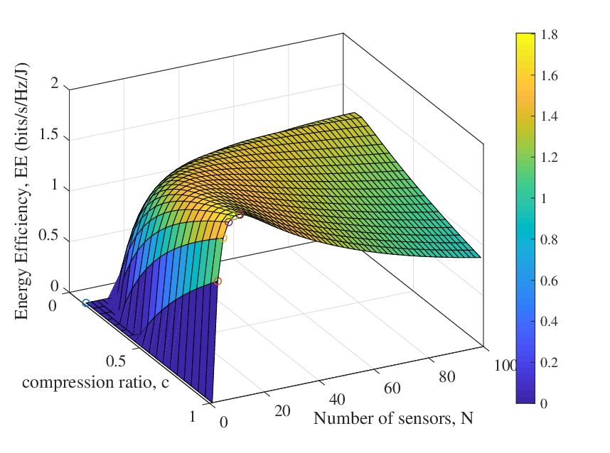
Figure 3: Energy efficiency as a function of number of sensors NN and compression ratio 𝚌\mathtt{c} for (a) deterministic signal case, SNR = −3-3 dB (b) random signal case SNR = −9-9 dB.
Refer to caption
(a) Deterministic PU signal.

Refer to caption
(b) Random signal.
Figure 4: Variation of the optimal compression ratio (𝚌∗\mathtt{c}^{*}) with number of sensors NN for (a) deterministic signal case (b) random signal case.
Refer to caption
(a) Deterministic PU signal.

Refer to caption
(b) Random PU signal.
Figure 5: Variation of the optimal number of sensors (N∗N^{*}) with compression ratio 𝚌∗\mathtt{c}^{*} for (a) deterministic signal case (b) random signal case.
Refer to caption
(a) Deterministic PU signal.

Refer to caption
(b) Random PU signal.
Figure 6: Variation of optimal energy efficiency with number of sensors NN for (a) deterministic signal case (b) random signal case.
Refer to caption
(a) Deterministic PU signal.

Refer to caption
(b) Random PU signal.
Figure 7: Variation of optimal achievable throughput with number of sensors NN for (a) deterministic signal case (b) random signal case.
Refer to caption
(a) Deterministic PU signal.

Refer to caption
(b) Random PU signal.
Figure 8: Variation of optimal energy consumption with number of sensors NN for (a) deterministic signal case (b) random signal case.

In this section, we study the performance of the CCCS technique in comparison with the CCS technique, in terms of energy efficiency and validate our analysis, through numerical techniques. The parameter values are fixed as follows. The target probability of detection, P¯d\overline{P}_{d}, and false-alarm probability, P¯f\overline{P}_{f}, are fixed to be 0.90.9 and 0.10.1, respectively. The prior probabilities π0\pi_{0} and π1\pi_{1} are set to be 0.50.5 each. The total frame duration is assumed to be TT​o​t​a​l=200T_{\scriptscriptstyle Total}=200 ms [23]. The sampling frequency at the local SUs is assumed to be fs=1f_{s}=1 MHz, and the sensing power Ps=0.1P_{s}=0.1 W. The length of the uncompressed received signal vector, P=100P=100. The sensing time, τs\tau_{s}, and reporting time, τr\tau_{r}, for the CCCS scheme are set to 3030 ms and 100100 μ\mus, respectively. The achievable rate of secondary transmission is chosen to be 𝒞=log2⁡(1+SNRs)=6.6582\mathcal{C}=\log_{2}(1+\text{SNR}_{s})=6.6582 bits/sec/Hz, where the SNR at the secondary receiver is assumed to be SNRs=20\text{SNR}_{s}=20 dB. The transmission power of individual sensors, PtP_{t}, is assumed to be 33 W. Also, we set the partial throughput factor, κc\kappa_{c}, and the penalty factor, ϕ\phi, to be 0.50.5 each.

Figure 3 shows the variation of energy efficiencies for the random and deterministic signal cases, as a function of parameters 𝚌\mathtt{c} and NN. Observe that the energy efficiency is concave in both 𝚌\mathtt{c} and NN. Furthermore, it can be seen that as NN increases, 𝚌\mathtt{c} decreases, which indicates a better compression. Also, the maximum energy efficiency can be improved with NN.

Figures 3(a) and 3(b) show the variation of the optimal compression ratio 𝚌∗\mathtt{c}^{*} for the CCCS scheme, as a function of NN for different values of SNR γ\gamma. First, note that the optimal values of 𝚌\mathtt{c} are nearly equal for the actual and approximate energy efficiency values, thereby establishing our earlier claim on the tightness of our approximations involved in evaluation of energy efficiency. The decrease in 𝚌∗\mathtt{c}^{*} with an increase in NN is intuitive, since the loss due to compression is recovered in CCCS by increasing NN, which results in a better throughput, and consequently, a better energy efficiency. Similarly, in Fig. 4(a) and 4(b), we consider the variation of optimal NN for different values of 𝚌\mathtt{c}, which yields similar trends and observations.

Figures 5(a) and 5(b) show the variation of optimal energy efficiency values with the actual and approximate expressions, for different values of NN. Note that for low values of NN, performances of both CCS and CCCS schemes are similar, due to the fact that 𝚌∗=1\mathtt{c}^{*}=1 for sufficiently low NN. As NN increases, the system achieves a better compression, and therefore, the performance of CCCS scheme becomes better than that of the CCS scheme. Also, the energy efficiency for both CCS and CCCS schemes increase with an increase in SNR. Moreover, the loss due to the energy efficiency approximation is negligible. Therefore, in our subsequent results, we consider only the approximated energy efficiency values. The reason for a better energy efficiency of the CCCS scheme in comparison to the CCS scheme can possibly be either because CCCS achieves a better throughput, or it achieves a lower energy consumption. Between these two cases, since the detection performance of the CCS scheme is better than that of CCCS scheme for a given NN (or 𝚌\mathtt{c}), the achievable throughput of the CCS scheme will always be higher as compared to that of the CCCS scheme. Therefore, the improvement in the energy efficiency of the CCCS scheme must be due to a significant reduction in energy consumption in comparison to the CCS scheme. Figures 7 and 8 corroborate this argument. In Fig. 7, the achievable throughput of CCS and CCCS schemes are compared, where the former is naturally found to be better. For larger values of NN, the detection probability and hence the throughput of the CCS scheme improves faster. However, as shown in Fig. 8, the energy consumption of the CCS scheme also increases rapidly with NN, as opposed to the CCCS scheme, where the increase is much slower since 𝚌∗\mathtt{c}^{*} decreases with NN. This is true for both random signal and deterministic signal cases. Hence, in scenarios where the energy consumption has a larger priority in a signal detection scenario CCCS scheme could be preferred. However, in the scenario where the sensing accuracy is a main concern, CCS scheme yields a better performance, in terms of energy efficiency.

VI Conclusion

We consider the energy efficiency of compressed conventional collaborative sensing (CCCS) scheme focusing on balancing the tradeoff between energy efficiency and detection accuracy in cognitive radio environment. We first consider the existing CCCS scheme in the literature, and derive the achievable throughput, energy consumption and energy efficiency. The energy efficiency maximization for the CCCS scheme is posed as a non-convex, optimization problem. We approximated the optimization problem to reduce it to a convex optimization problem, and showed that this approximation holds with sufficient accuracy in the regime of interest. We analytically characterize the tradeoff between dimensionality reduction and collaborative sensing of CCCS scheme – the implicit tradeoff between energy saving and detection accuracy, and show that by combining compression and collaboration the loss due to one can be compensated by the other which improves the overall energy efficiency of the cognitive radio network.

VII Appendix

VII-A Proof of Theorem 1

To establish that PdC​C​C​S≥P¯dP_{\scriptstyle d}^{\scriptscriptstyle CCCS}\geq\overline{P}_{d} is satisfied with equality, we show that ∂E​E~c​c​c​s​(λ,𝚌,N)∂λ≥0\frac{\partial\tilde{EE}_{\scriptscriptstyle cccs}(\lambda,\mathtt{c},N)}{\partial\lambda}\geq 0, for all λ\lambda. Observe that

∂E​E~c​c​c​s​(λ,𝚌,N)∂λ=∂R~c​c​c​s​(λ)∂λ​E~c​c​c​s​(λ)−R~c​c​c​s​(λ)​∂E~c​c​c​s​(λ)∂λE~c​c​c​s2​(λ),\displaystyle\frac{\partial\tilde{EE}_{\scriptscriptstyle cccs}(\lambda,\mathtt{c},N)}{\partial\lambda}=\frac{\frac{\partial\tilde{R}_{\scriptscriptstyle cccs}(\lambda)}{\partial\lambda}\tilde{E}_{\scriptscriptstyle cccs}(\lambda)-\tilde{R}_{\scriptscriptstyle cccs}(\lambda)\frac{\partial\tilde{E}_{\scriptscriptstyle cccs}(\lambda)}{\partial\lambda}}{\tilde{E}_{\scriptscriptstyle cccs}^{2}(\lambda)}, (43)

where

∂R~c​c​c​s​(λ,𝚌,N)∂λ=−∂Pf∂λ​(1+ϕ)​π0​𝒞​(TT​o​t​a​l−𝚌​Ts),\displaystyle\frac{\partial\tilde{R}_{\scriptscriptstyle cccs}(\lambda,\mathtt{c},N)}{\partial\lambda}=-\frac{\partial P_{f}}{\partial\lambda}(1+\phi)\pi_{0}\mathcal{C}(T_{\scriptscriptstyle Total}-\mathtt{c}T_{s}), (44)

and

∂E~c​c​c​s​(λ,𝚌,N)∂λ=−∂Pf∂λ​π0​Pt​(TT​o​t​a​l−𝚌​Ts).\displaystyle\frac{\partial\tilde{E}_{\scriptscriptstyle cccs}(\lambda,\mathtt{c},N)}{\partial\lambda}=-\frac{\partial P_{f}}{\partial\lambda}\pi_{0}P_{t}(T_{\scriptscriptstyle Total}-\mathtt{c}T_{s}). (45)

Upon further simplification, we get

∂E~c​c​c​s​(λ,𝚌,N)∂λ=−∂Pf∂λ​V1​(λ,𝚌,N),\displaystyle\frac{\partial\tilde{E}_{\scriptscriptstyle cccs}(\lambda,\mathtt{c},N)}{\partial\lambda}=-\frac{\partial P_{f}}{\partial\lambda}V_{1}(\lambda,\mathtt{c},N), (46)

where

V1(λ,𝚌,N)=[(1+ϕ)​π0​𝒞​(TT​o​t​a​l−𝚌​Ts)​E~c​c​c​s​(λ,𝚌,N)E~c​c​c​s2​(λ,𝚌,N)\displaystyle V_{1}(\lambda,\mathtt{c},N)=\left[\hskip-2.84544pt\frac{(1+\phi)\pi_{0}\mathcal{C}(T_{\scriptscriptstyle Total}-\mathtt{c}T_{s})\tilde{E}_{\scriptscriptstyle cccs}(\lambda,\mathtt{c},N)}{\tilde{E}_{\scriptscriptstyle cccs}^{2}(\lambda,\mathtt{c},N)}\right.
−π0​Pt​(TT​o​t​a​l−𝚌​Ts)∗R~c​c​c​s​(λ,c,N)E~c​c​c​s2​(λ,𝚌,N)]\displaystyle\penalty\ \penalty\ \penalty\ \penalty\ \penalty\ \penalty\ \penalty\ \penalty\ \penalty\ \penalty\ \penalty\ \penalty\ \penalty\ \penalty\ \penalty\ \penalty\ \penalty\ \penalty\ \left.-\frac{\pi_{0}P_{t}(T_{\scriptscriptstyle Total}-\mathtt{c}T_{s})*\tilde{R}_{\scriptscriptstyle cccs}(\lambda,c,N)}{\tilde{E}_{\scriptscriptstyle cccs}^{2}(\lambda,\mathtt{c},N)}\right] (47)

Now, to show that ∂E​EC​C​C​S​(λ,𝚌,N)∂λ≥0\frac{\partial EE_{\scriptscriptstyle CCCS}(\lambda,\mathtt{c},N)}{\partial\lambda}\geq 0, it is enough to show that V1​(λ,𝚌,N)≥0V_{1}(\lambda,\mathtt{c},N)\geq 0, since

∂Pf∂λ=−12​σw2​𝚌​N​P​π​exp⁡[−(λσw2−𝚌​N​P)2(4​𝚌​N​P)]≤0.\displaystyle\frac{\partial P_{f}}{\partial\lambda}=-\frac{1}{2\sigma_{w}^{2}\sqrt{\mathtt{c}NP\pi}}\exp\left[-\frac{\left(\frac{\lambda}{\sigma_{w}^{2}}-\mathtt{c}NP\right)^{2}}{(4\mathtt{c}NP)}\right]\leq 0.

In general, it is hard to analytically show that V1​(λ,𝚌,N)≥0V_{1}(\lambda,\mathtt{c},N)\geq 0. However, since R~c​c​c​s​(λ,𝚌,N)≥0\tilde{R}_{\scriptscriptstyle cccs}(\lambda,\mathtt{c},N)\geq 0 and E~c​c​c​s​(λ,𝚌,N)≥0\tilde{E}_{\scriptscriptstyle cccs}(\lambda,\mathtt{c},N)\geq 0, the parameters ϕ,𝒞,TT​o​t​a​l\phi,\mathcal{C},T_{\scriptscriptstyle Total} and TsT_{s} can be chosen such that (1+ϕ)​π0​𝒞​(TT​o​t​a​l−𝚌​Ts)​E~c​c​c​s​(λ,𝚌,N)≥π0​Pt​(TT​o​t​a​l−𝚌​Ts)​R~c​c​c​s​(λ,𝚌,N)(1+\phi)\pi_{0}\mathcal{C}(T_{\scriptscriptstyle Total}-\mathtt{c}T_{s})\tilde{E}_{\scriptscriptstyle cccs}(\lambda,\mathtt{c},N)\geq\pi_{0}P_{t}(T_{\scriptscriptstyle Total}-\mathtt{c}T_{s})\tilde{R}_{\scriptscriptstyle cccs}(\lambda,\mathtt{c},N). Later, in Sec. V, it can be seen that the above condition is satisfied for those parameter values which are of practical interest. Therefore,

P¯d=Q⁡(λ∗σx2+σw2−𝚌​N​P2​𝚌​N​P)\displaystyle\overline{P}_{d}=Q\left(\frac{\frac{\lambda^{*}}{\sigma_{x}^{2}+\sigma_{w}^{2}}-\mathtt{c}NP}{\sqrt{2\mathtt{c}NP}}\right)
=Q⁡(λ∗σw2​(11+γ)−𝚌​N​P2​𝚌​N​P).\displaystyle\phantom{\overline{P}_{d}}=Q\left(\frac{\frac{\lambda^{*}}{\sigma_{w}^{2}}\left(\frac{1}{1+\gamma}\right)-\mathtt{c}NP}{\sqrt{2\mathtt{c}NP}}\right). (48)

Rearranging the equation gives the expression for λ∗\lambda^{*}.

VII-B Proof of Theorem 2

Note that

∂E​E~c​c​c​s​(λ,𝚌,N)∂𝚌=∂R~c​c​c​s​(𝚌)∂𝚌​E~c​c​c​s​(𝚌)−R~c​c​c​s​(𝚌)​∂E~c​c​c​s​(𝚌)∂𝚌E~c​c​c​s2​(𝚌).\displaystyle\frac{\partial\tilde{EE}_{\scriptscriptstyle cccs}(\lambda,\mathtt{c},N)}{\partial\mathtt{c}}=\frac{\frac{\partial\tilde{R}_{\scriptscriptstyle cccs}(\mathtt{c})}{\partial\mathtt{c}}\tilde{E}_{\scriptscriptstyle cccs}(\mathtt{c})-\tilde{R}_{\scriptscriptstyle cccs}(\mathtt{c})\frac{\partial\tilde{E}_{\scriptscriptstyle cccs}(\mathtt{c})}{\partial\mathtt{c}}}{\tilde{E}_{\scriptscriptstyle cccs}^{2}(\mathtt{c})}. (49)

As 𝚌→0\mathtt{c}\rightarrow 0, it can be shown that

lim𝚌→0​∂E​E~c​c​c​s​(λ,𝚌,N)∂𝚌≥lim𝚌→0​{−∂Pf∂𝚌​(𝒞Pt)+V2​(𝚌,N)},\displaystyle\underset{\mathtt{c}\rightarrow 0}{\lim}\frac{\partial\tilde{EE}_{\scriptscriptstyle cccs}(\lambda,\mathtt{c},N)}{\partial\mathtt{c}}\geq\underset{\mathtt{c}\rightarrow 0}{\lim}\left\{-\frac{\partial P_{f}}{\partial\mathtt{c}}\left(\frac{\mathcal{C}}{P_{t}}\right)+V_{2}(\mathtt{c},N)\right\}, (50)

where

V2​(𝚌,N)=[N​Ps​τs+N​Pt​τr]​π0​𝒞Pt2≥0\displaystyle V_{2}(\mathtt{c},N)=\frac{\left[NP_{s}\tau_{s}+NP_{t}\tau_{r}\right]\pi_{0}\mathcal{C}}{P_{t}^{2}}\geq 0 (51)

Also, note that

∂Pf∂𝚌=−1π​exp⁡((λ∗σw2−𝚌​N​P)24​𝚌​N​P)\displaystyle\frac{\partial P_{f}}{\partial\mathtt{c}}=-\frac{1}{\sqrt{\pi}}\exp\left(\frac{(\frac{\lambda^{*}}{\sigma_{w}^{2}}-\mathtt{c}NP)^{2}}{4\mathtt{c}NP}\right)
[−N​P2​𝚌​N​P−N​P​((λ∗σw2−𝚌​N​P))4​(𝚌​N​P3/2)]\displaystyle\penalty\ \penalty\ \penalty\ \penalty\ \penalty\ \penalty\ \penalty\ \penalty\ \penalty\ \penalty\ \penalty\ \penalty\ \penalty\ \penalty\ \penalty\ \penalty\ \left[-\frac{NP}{2\sqrt{\mathtt{c}NP}}-\frac{NP((\frac{\lambda^{*}}{\sigma_{w}^{2}}-\mathtt{c}NP))}{4(\mathtt{c}NP^{3/2})}\right] (52)

Therefore, PfP_{f} is a monotonically decreasing function of 𝚌\mathtt{c}. When 𝚌→0\mathtt{c}\rightarrow 0, it can be shown that ∂Pf​(λ,𝚌,N)∂𝚌→−∞\frac{\partial P_{f}(\lambda,\mathtt{c},N)}{\partial\mathtt{c}}\rightarrow-\infty. Since V2​(𝚌,N)V_{2}(\mathtt{c},N) is a positive constant, lim𝚌→0​∂E​E~c​c​c​s​(λ,𝚌,N)∂𝚌=+∞\underset{\mathtt{c}\rightarrow 0}{\lim}\frac{\partial\tilde{EE}_{\scriptscriptstyle cccs}(\lambda,\mathtt{c},N)}{\partial\mathtt{c}}=+\infty. Furthermore, using a well-known bound on the Q function, we get the following lower bound PfP_{f} as

Pf≥[1−2​c​N​P(λσw2−c​N​P)2]​exp−[(λσw2−c​N​P)24​c​N​P],\displaystyle P_{f}\geq\left[1-\frac{2cNP}{(\frac{\lambda}{\sigma_{w}^{2}}-cNP)^{2}}\right]\exp{-\left[\frac{(\frac{\lambda}{\sigma_{w}^{2}}-cNP)^{2}}{4cNP}\right]}, (53)

which can be used to get a lower bound on the first derivative of E​E~c​c​c​s​(λ,𝚌,N)\tilde{EE}_{\scriptscriptstyle cccs}(\lambda,\mathtt{c},N) as

∂E​E~c​c​c​s​(λ,𝚌,N)∂𝚌≥(B​A−B​D−B​C−A​E)⏟≜X1\displaystyle\frac{\partial\tilde{EE}_{\scriptscriptstyle cccs}(\lambda,\mathtt{c},N)}{\partial\mathtt{c}}\geq\underbrace{(BA-BD-BC-AE)}_{\triangleq X_{1}}
+(B​C+A​E−2​B​A+2​B​D)​[1−2​c​N​P(λσw2−c​N​P)2]​e−[(λσw2−c​N​P)24​c​N​P]⏟≜X2\displaystyle\hskip-8.5359pt+\underbrace{(BC+AE-2BA+2BD)\left[1-\frac{2cNP}{(\frac{\lambda}{\sigma_{w}^{2}}-cNP)^{2}}\right]e^{-\left[\frac{(\frac{\lambda}{\sigma_{w}^{2}}-cNP)^{2}}{4cNP}\right]}}_{\triangleq X_{2}}
+(B​A−B​D)​[1−2​c​N​P(λσw2−c​N​P)2]2​e−[(λσw2−c​N​P)24​c​N​P]⏟≜X3\displaystyle\hskip-2.84544pt+\underbrace{(BA-BD)\left[1-\frac{2cNP}{(\frac{\lambda}{\sigma_{w}^{2}}-cNP)^{2}}\right]^{2}e^{-\left[\frac{(\frac{\lambda}{\sigma_{w}^{2}}-cNP)^{2}}{4cNP}\right]}}_{\triangleq X_{3}}
−(A​C)​∂Pf​(λ,𝚌,N)∂𝚌⏟≜X4,\displaystyle-\underbrace{(AC)\frac{\partial P_{f}(\lambda,\mathtt{c},N)}{\partial\mathtt{c}}}_{\triangleq X_{4}}, (54)

where A=π0​𝒞​[TT​o​t​a​l−𝚌​Ts]≥0A=\pi_{0}\mathcal{C}\left[T_{\scriptscriptstyle Total}-\mathtt{c}T_{s}\right]\geq 0, B=π0​Pt​Ts≥0B=\pi_{0}P_{t}T_{s}\geq 0, C=N​Ps​𝚌​τs+N​Pt​𝚌​τr≥0C=NP_{s}\mathtt{c}\tau_{s}+NP_{t}\mathtt{c}\tau_{r}\geq 0, and D=Pt​[TT​o​t​a​l−𝚌​Ts]​π0≥0D=P_{t}\left[T_{\scriptscriptstyle Total}-\mathtt{c}T_{s}\right]\pi_{0}\geq 0.

As seen earlier, ∂Pf∂𝚌\frac{\partial P_{f}}{\partial\mathtt{c}} is negative, and it is easy to show that B​C+A​E−2​B​A+2​B​D>0,B​A−B​D>0BC+AE-2BA+2BD>0,BA-BD>0, and consequently, X2≥0X_{2}\geq 0, X3≥0X_{3}\geq 0 and X4≥0X_{4}\geq 0. Now,

∂E​E~c​c​c​s​(λ,𝚌,N)∂𝚌≥X1+X2+X3+X4\displaystyle\frac{\partial\tilde{EE}_{\scriptscriptstyle cccs}(\lambda,\mathtt{c},N)}{\partial\mathtt{c}}\geq X_{1}+X_{2}+X_{3}+X_{4}
≥X1\displaystyle\penalty\ \penalty\ \geq X_{1}
=B​A−B​D−B​C−A​E\displaystyle\penalty\ \penalty\ =BA-BD-BC-AE
=(π02​Pt​Ts)​π0​𝒞​(TT​o​t​a​l−𝚌​Ts)−(π02​Pt2​Ts)​(TT​o​t​a​l−𝚌​Ts)\displaystyle\penalty\ \penalty\ =(\pi_{0}^{2}P_{t}T_{s})\pi_{0}\mathcal{C}(T_{\scriptscriptstyle Total}-\mathtt{c}T_{s})-(\pi_{0}^{2}P_{t}^{2}T_{s})(T_{\scriptscriptstyle Total}-\mathtt{c}T_{s})
−(π0​Pt​Ts)​(N​Ps​c​τs+N​Pt​c​τr)\displaystyle\penalty\ \penalty\ \penalty\ \penalty\ \penalty\ \penalty\ \penalty\ \penalty\ \penalty\ -(\pi_{0}P_{t}T_{s})(NP_{s}c\tau_{s}+NP_{t}c\tau_{r})
OPEN−π0​𝒞​(TT​o​t​a​l−𝚌​Ts)​(N​Ps​τs+N​Pt​τr))\displaystyle\penalty\ \penalty\ \penalty\ \penalty\ \penalty\ \penalty\ \penalty\ \penalty\ \penalty\ -\hskip-2.84544pt\pi_{0}\hskip-0.28436pt\mathcal{C}(T_{\scriptscriptstyle Total}-\mathtt{c}T_{s})(NP_{s}\tau_{s}+\hskip-2.84544ptNP_{t}\tau_{r}))
=π0​{Pt​Ts​𝒞−Pt2​Ts−𝒞⁡(N​Ps​τs+N​Pt​τr)}⏟≜W​(TT​o​t​a​l−𝚌​Ts)\displaystyle\penalty\ \penalty\ =\underbrace{\pi_{0}\left\{P_{t}T_{s}\mathcal{C}-P_{t}^{2}T_{s}-\mathcal{C}(NP_{s}\tau_{s}+NP_{t}\tau_{r})\right\}}_{\triangleq W}(T_{\scriptscriptstyle Total}\hskip-2.84544pt-\hskip-2.84544pt\mathtt{c}T_{s})
−𝚌​π0​Pt​Ts​(N​Ps​τs+N​Pt​τr)⏟≜Y\displaystyle\penalty\ \penalty\ \penalty\ \penalty\ \penalty\ \penalty\ \penalty\ \penalty\ \penalty\ \penalty\ -\mathtt{c}\underbrace{\pi_{0}P_{t}T_{s}(NP_{s}\tau_{s}+NP_{t}\tau_{r})}_{\triangleq Y} (55)

To ensure that ∂E​E~c​c​c​s​(λ,𝚌,N)∂𝚌≥0\frac{\partial\tilde{EE}_{\scriptscriptstyle cccs}(\lambda,\mathtt{c},N)}{\partial\mathtt{c}}\geq 0, we need that the right hand side of (55) to be ≥0\geq 0. Rearranging (55), observe that this is true when 𝚌≤𝚌U​B≜TT​o​t​a​l​WTs​W+Y\mathtt{c}\leq\mathtt{c}_{\scriptscriptstyle\text{$UB$}}\triangleq\frac{T_{\scriptscriptstyle Total}W}{T_{s}W+Y}. In other words, we have shown that ∂E​E~c​c​c​s​(λ,𝚌,N)∂𝚌≥0\frac{\partial\tilde{EE}_{\scriptscriptstyle cccs}(\lambda,\mathtt{c},N)}{\partial\mathtt{c}}\geq 0 whenever 𝚌∈(0,𝚌U​B)\mathtt{c}\in(0,\mathtt{c}_{\scriptscriptstyle\text{$UB$}}). Finally, to establish that 𝚌∗=𝚌max\mathtt{c}^{*}=\mathtt{c}_{\scriptscriptstyle\text{$\max$}}, we need to show that 𝚌max≤𝚌U​B\mathtt{c}_{\scriptscriptstyle\text{$\max$}}\leq\mathtt{c}_{\scriptscriptstyle\text{$UB$}}. Although hard to show analytically, it is verified to be indeed true numerically, for moderate values of NN and for low SNR, which is of practical relevance.

VII-C Proof of Theorem 4

Note that the first derivative of PfP_{f} is negative as given below.

∂Pf∂λ=−1σw2​2​π​𝚌​N​γ​exp⁡[−λ2(2​𝚌​N​γ​σw4)]≤0\displaystyle\frac{\partial P_{f}}{\partial\lambda}=-\frac{1}{\sigma_{w}^{2}\sqrt{2\pi\mathtt{c}N\gamma}}\exp\left[\frac{-\lambda^{2}}{(2\mathtt{c}N\gamma\sigma_{w}^{4})}\right]\leq 0 (56)

As mentioned earlier, since the expressions for average achievable throughput, average energy consumption and the energy efficiency expressions across all four scenarios S1−S4\textbf{S1}-\textbf{S4} for the deterministic case remains similar to the previous case, and similar set of arguments hold true for the deterministic case too. These can be used to prove that the first derivative of E​E~c​c​c​s\tilde{EE}_{\scriptscriptstyle cccs} is greater than or equal to 00. Therefore,

P¯d=Q⁡(λ∗−𝚌​N​σw2σw2​𝚌​N​γ).\displaystyle\overline{P}_{d}=Q\left(\frac{{\lambda^{*}}-\mathtt{c}N\sigma_{w}^{2}}{\sigma_{w}^{2}\sqrt{\mathtt{c}N\gamma}}\right). (57)

Rearranging the above equation gives the expression for λ∗\lambda^{*}.

VII-D Proof of Theorem 5

Note that the first derivative of PfC​C​C​S,d​e​tP_{\scriptstyle f}^{\scriptscriptstyle CCCS,det} with respect to 𝚌\mathtt{c} from (34) is given by,

∂Pf​(λ,N,𝚌)∂𝚌=−exp⁡(−(λ22​N​γ​σw4)​N​γ​λCLOSE2​2​π​(c​N​γ)3/2​σw2≤0.\frac{\partial P_{f}(\lambda,N,\mathtt{c})}{\partial\mathtt{c}}=-\frac{\exp(-(\frac{\lambda^{2}}{2N\gamma\sigma_{w}^{4}})N\gamma\lambda}{2\sqrt{2\pi}(cN\gamma)^{3/2}\sigma_{w}^{2}}\leq 0. (58)

Therefore, lim𝚌→0​∂Pf​(λ,𝚌,N)∂𝚌→−∞\underset{\mathtt{c}\rightarrow 0}{\lim}\frac{\partial P_{f}(\lambda,\mathtt{c},N)}{\partial\mathtt{c}}\rightarrow-\infty. Similar arguments given in Sec. VII-B can be used to show that 𝚌∗=𝚌max\mathtt{c}^{*}=\mathtt{c}_{\scriptscriptstyle\text{$\max$}}, even in this case.

References

  • [1] R. Kishore, S. Gurugopinath, S. Muhaidat, P. C. Sofotasios, M. Dianati, and N. Al-Dhahir, “Energy efficiency analysis of collaborative compressive sensing for cognitive radio networks,” in Proc. GLOBECOM, Dec. 2018, pp. 1–6.
  • [2] M. M. Mowla, I. Ahmad, D. Habibi, and Q. V. Phung, “A green communication model for 5G systems,” IEEE Trans. Cognitive Commun. Netw., vol. 1, no. 3, pp. 264–280, Sep. 2017.
  • [3] X. Huang, T. Han, and N. Ansari, “On green-energy-powered cognitive radio networks,” IEEE Commun. Surveys Tuts., vol. 17, no. 2, pp. 827–842, Second quarter 2015.
  • [4] M. Zheng, L. Chen, W. Liang, H. Yu, and J. Wu, “Energy-efficiency maximization for cooperative spectrum sensing in cognitive sensor networks,” IEEE Trans. Cognitive Commun. Netw., vol. 1, no. 1, pp. 29–39, Mar. 2017.
  • [5] M. Yousefvand, T. Han, N. Ansari, and A. Khreishah, “Distributed energy-spectrum trading in green cognitive radio cellular networks,” IEEE Trans. Cognitive Commun. Netw., vol. 1, no. 3, pp. 253–263, Sep. 2017.
  • [6] T. Yucek and H. Arslan, “A survey of spectrum sensing algorithms for cognitive radio applications,” IEEE Commun. Surveys Tuts., vol. 11, no. 1, pp. 116–130, First quarter 2009.
  • [7] J. M. Bruno and B. L. Mark, “A recursive algorithm for wideband temporal spectrum sensing,” IEEE Trans. Commun., vol. 66, no. 1, pp. 26–38, Jan. 2018.
  • [8] K. Cao, P. Lu, C. Sun, Y. Zou, J. Wang, and L. Ling, “Frequency locator polynomial for wideband sparse spectrum sensing with multichannel subsampling,” IEEE Trans. Signal Process., vol. 66, no. 3, pp. 789–803, Feb. 2018.
  • [9] A. Ali and W. Hamouda, “Power-efficient wideband spectrum sensing for cognitive radio systems,” IEEE Trans. Veh. Technol., vol. 67, no. 4, pp. 3269–3283, Apr. 2018.
  • [10] T. Xiong, H. Li, P. Qi, Z. Li, and S. Zheng, “Predecision for wideband spectrum sensing with sub-nyquist sampling,” IEEE Trans. Veh. Technol., vol. 66, no. 8, pp. 6908–6920, Aug. 2017.
  • [11] J. Zhao, Q. Liu, X. Wang, and S. Mao, “Scheduled sequential compressed spectrum sensing for wideband cognitive radios,” IEEE Trans. Mobile Comput., vol. 17, no. 4, pp. 913–926, Apr. 2018.
  • [12] S. K. Sharma, E. Lagunas, S. Chatzinotas, and B. Ottersten, “Application of compressive sensing in cognitive radio communications: A survey,” IEEE Commun. Surveys Tuts., vol. 18, no. 3, pp. 1838–1860, Third quarter 2016.
  • [13] F. Salahdine, N. Kaabouch, and H. E. Ghazi, “A survey on compressive sensing techniques for cognitive radio networks,” Physical Communication, vol. 20, pp. 61 – 73, Sep. 2016.
  • [14] Y. Ma, Y. Gao, A. Cavallaro, C. G. Parini, W. Zhang, and Y. C. Liang, “Sparsity independent sub-Nyquist rate wideband spectrum sensing on real-time TV white space,” IEEE Trans. Veh. Technol., vol. 66, no. 10, pp. 8784–8794, Oct. 2017.
  • [15] L. Arienzo and D. Tarchi, “Stochastic optimization of cognitive networks,” IEEE Trans. Green Commun. Netw., vol. 1, no. 1, pp. 40–58, Mar. 2017.
  • [16] B. Kailkhura, T. Wimalajeewa, and P. K. Varshney, “Collaborative compressive detection with physical layer secrecy constraints,” IEEE Trans. Signal Process., vol. 65, no. 4, pp. 1013–1025, Feb. 2017.
  • [17] Q. Zhao, Z. Wu, and X. Li, “Energy efficiency of compressed spectrum sensing in wideband cognitive radio networks,” EURASIP Journal on Wireless Communications and Networking, vol. 2016, no. 1, p. 83, Mar. 2016.
  • [18] C. R. Stevenson, G. Chouinard, Z. Lei, W. Hu, S. J. Shellhammer, and W. Caldwell, “IEEE 802.22: The first cognitive radio wireless regional area network standard,” Comm. Mag., vol. 47, no. 1, pp. 130–138, Jan. 2009.
  • [19] E. C. Y. Peh, Y. C. Liang, Y. L. Guan, and Y. Pei, “Energy-efficient cooperative spectrum sensing in cognitive radio networks,” in Proc. GLOBECOM, Dec. 2011, pp. 1–5.
  • [20] Y. Gao, W. Xu, K. Yang, K. Niu, and J. Lin, “Energy-efficient transmission with cooperative spectrum sensing in cognitive radio networks,” in Proc. WCNC, Apr. 2013, pp. 7–12.
  • [21] H. Urkowitz, “Energy detection of unknown deterministic signals,” Proc. IEEE, vol. 55, no. 4, pp. 523–531, Apr. 1967.
  • [22] N. Reisi, V. Jamali, and M. Ahmadian, “Linear decision fusion based cooperative spectrum sensing in cognitive radio networks,” in Proc. AISP (International Symposium on Artifical Intelligence and Signal Processing), May 2012, pp. 211–215.
  • [23] R. Kishore, C. K. Ramesha, S. Gurugopinath, and K. R. Anupama, “Performance analysis of superior selective reporting-based energy efficient cooperative spectrum sensing in cognitive radio networks,” Ad Hoc Networks, vol. 65, pp. 99 – 116, Oct. 2017.