Randomized Discrete Empirical Interpolation Method for Nonlinear Model Reduction
Abstract
Discrete empirical interpolation method (DEIM) is a popular technique for nonlinear model reduction and it has two main ingredients: an interpolating basis that is computed from a collection of snapshots of the solution, and a set of indices which determine the nonlinear components to be simulated. The computation of these two ingredients dominates the overall cost of the DEIM algorithm. To specifically address these two issues, we present randomized versions of the DEIM algorithm. There are three main contributions of this paper. First, we use randomized range finding algorithms to efficiently find an approximate DEIM basis. Second, we develop randomized subset selection tools, based on leverage scores, to efficiently select the nonlinear components. Third, we develop several theoretical results that quantify the accuracy of the randomization on the DEIM approximation. We also present numerical experiments that demonstrate the benefits of the proposed algorithms.
1 Introduction
Detailed mathematical models of weather prediction and neuroscience routinely generate large-scale problems having over a billion unknowns. The goal of model reduction is to replace computationally expensive full-scale models by reduced order models (ROMs) that are cheaper to evaluate and that preserve the important underlying physics in the full-scale models. Development of effective ROMs will enable efficient and accurate simulation of a wide range of detailed complex physical phenomena, as well as benefit a host of applications in inverse problems, data assimilation, design, control, optimization, and uncertainty quantification.
In a typical model reduction technique, there are two distinct phases: an offline phase in which the full model is simulated for a range of parameters or specifications and the outputs of this simulations are used to construct the ROM, and an online phase, in which the ROM is simulated for the desired parameter, or specification. A successful ROM has two features that are hard to achieve simultaneously: the ROM should be accurate over the desired range of parameters and specifications, and the online phase should be inexpensive and the dominant computational cost should be in the offline phase. A popular method for model reduction is the proper orthogonal decomposition (POD), which has been successfully used in a wide range of partial differential equation (PDE)-based applications, and is reviewed in section 2.1. While POD approach has broad applicability, the computational efficiency of the POD demands that the underlying PDE has to be linear, or the parameter dependence has to be of a specific type, e.g., affine parameter dependence. To address this deficiency, many methods have been proposed in the literature such as gappy POD interpolation method, empirical interpolation method (EIM), and its discrete variant, the discrete empirical interpolation method (DEIM). Reviews of various model reduction techniques are provided in the survey paper [3], recent books and monographs [17, 25].
The DEIM interpolation framework computes an approximation of a nonlinear function by the means of a basis used to interpolate the function, and a set of indices, defining a point selection operator , at which the nonlinear function is evaluated. In section 2.2, we explain how and can be used to approximate the function ; here, we describe the major bottlenecks in computing the DEIM approximation.
- •
The basis is constructed as follows: several representative samples—also called as snapshots—of the function are collected and arranged as columns of a matrix, known as the snapshot matrix. The left singular vectors of this snapshot matrix form the desired DEIM basis—henceforth, we call this the standard basis. The dimension of the subspace spanned by the DEIM basis, denoted by , depends on the number of dominant singular values of the snapshot matrix. Computing a truncated singular value decomposition (SVD) costs , where is the number of snapshots; our approach replaces the SVD by a randomized SVD.
- •
Finding a set of good indices is a combinatorially hard problem known as subset selection (in the DEIM literature, this is known as point selection, which we also adopt in this manuscript). Various deterministic subset selection techniques have been proposed in the literature: based on pivoted LU factorization [7, 28], pivoted QR factorization [9], strong rank-revealing QR factorization [10]. The computational cost is roughly ; we use randomized subset selection techniques which lowers this cost and can exploit parallelism.
Both of these operations are computationally expensive when is large. Our paper specifically addresses these computational challenges using randomized algorithms, thereby enabling efficient large-scale implementation of DEIM.
To motivate the development of randomized algorithm for DEIM, we briefly review randomized algorithms in other applications. Recently, randomized algorithms have been developed for accurate low-rank approximations to matrices arising from large datasets. The basic idea of these methods is to use random sampling to identify a subspace which approximately captures the range of the matrix [16]. The matrix is then projected onto this subspace and then deterministic linear algebraic techniques can be used to manipulate the projected matrix to obtain the desired low-rank approximation. Besides low-rank approximations, randomized methods (based on leverage score sampling and other subset selection techniques) have been developed for other linear algebraic problems such as least squares problems, regression, and computation of interpretable decompositions such as CX/CUR decompositions, see recent survey articles [20, 8]. Randomized methods have several advantages over their corresponding classical counterparts: typically, they are computationally efficient, numerically robust, easy to implement, scale well in a distributed computing setting, and have well-developed error analysis.
Contributions and Contents
We present randomized algorithms for DEIM that enable nonlinear dimensionality reduction for several large-scale applications.
We present randomized approaches (section 3) for efficient construction of a DEIM basis . The algorithms come in two flavors depending on whether the target rank is known or not. When the target rank is known, we present a basic version and a more accurate version based on subspace iteration. When the target rank is unknown, we provide an adaptive algorithm for computing . The computational and storage advantages of the randomized algorithms for constructing the DEIM basis are highlighted.
We present a detailed analysis of the error (section 4) when a randomized basis instead of the standard DEIM basis. A crucial component of our analysis involves the largest canonical angle between the subspaces spanned by the standard basis , and an approximate basis . This analysis is applicable to any approximate basis and therefore this has broad appeal beyond the context of randomized algorithms. We also present specific results that explicitly account for the randomness on the accuracy of the DEIM approximation.
We propose two randomized point selection methods for DEIM approximation (section 5): leverage score sampling and hybrid algorithms. For each method, we present theoretical bounds on the number of points required for the desired accuracy. The hybrid point selection technique combines the computational advantages of the randomized methods with the accuracy of deterministic methods. These sampling methods have been proposed in the context of matrix CUR decompositions; our analysis for the DEIM approximation is new.
Numerical experiments (section 6) demonstrate the computational benefits, the accuracy of the randomized approaches and insight into the choice of parameters for various algorithms presented in this paper.
Related work
The idea of using randomization to accelerate computations in model reduction appears to be relatively new and here we briefly review the literature. Randomized matrix methods, similar to the ones used in this paper, have been used to approximate POD [33, 34, 2], and dynamic mode decomposition [12, 11, 4]. Recent work in [1] uses randomization for reducing the cost associated with multiple right hand sides in nonlinear model reduction. The resulting ROM dramatically reduces the cost of solving a PDE-based inverse problem. However, none of these references directly tackle the DEIM approximation, which is the central focus of this paper. Randomized sampling approaches for choosing the DEIM indices have been proposed in [9] but no analysis of the randomization was presented. Another noteworthy paper [23], uses randomized oversampling to address stability issues with DEIM.
2 Preliminaries
We briefly review the POD and DEIM approaches for model order reduction.
2.1 Proper Orthogonal Decomposition
We explain the POD approach in the context of a nonlinear dynamical system that takes the form
| (1) |
where . When is large, the simulation of the dynamical system can be computationally expensive, and we turn to reduced order models to lower the computational cost. In the POD approach, the dynamical system is first simulated numerically and the “snapshots” of the system at multiple times , as for are collected into the POD snapshot matrix
We then compute its thin SVD . The POD approach chooses the singular vectors corresponding to the largest singular values, collected in a matrix (using MATLAB notation). The basis, thus obtained, also solves the following optimization problem
| (2) |
where are the singular values of . The choice of snapshots is an important issue in determining an effective POD basis and is discussed in [25, 3, 17]. Assuming that we have an effective basis , the solution can be approximated to be constrained in the span of the basis of the columns of , i.e., . Next, the reduced system is obtained by a Galerkin projection onto ; the dynamics of is given by
This approach, known as the POD-Galerkin method, is an effective way of reducing the dimensionality of the system of equations represented in eq. 1. This approach is more generally applicable to other applications such as parameterized PDEs.
We briefly discuss the computational cost of the POD-Galerkin approach. Note that the matrix can be precomputed. If the nonlinear term , then the cost of simulating the reduced system for is independent of , the dimension of the full order system. However, the evaluation of the nonlinear term has computational complexity that depends on . As a result, evaluation of this term may still be as expensive as solving the original system.
2.2 DEIM approximation
The DEIM approximation was proposed to address the deficiency of POD-Galerkin approach for nonlinear dynamical systems. Given a collection of snapshots of the full order dynamical system
a projection basis is computed by retaining the left-singular vectors corresponding to the top- singular values. We denote this standard DEIM basis by . The DEIM approach then selects distinct rows from the matrix ; in particular, denoting the row indices we define the selection operator
where is the -th column of the identity matrix.
We define the DEIM projector that satisfies (i.e., is idempotent) and if and , then
| (3) |
The equality follows from the property of oblique projectors [30]. Since and have orthonormal columns and is unitarily invariant, we also have the equality . Given the DEIM projector, the DEIM approximation of can be expressed as
| (4) |
We recapitulate a few properties of the DEIM projector that will be useful in subsequent analysis. Let and be two orthogonal projectors corresponding to the bases and respectively. Suppose that . The following relations hold
| (5) | ||||||
| (6) | ||||||
| (7) | ||||||
Remark 1.
In the original DEIM approach [7], the number of selected indices equals the dimension of the DEIM basis . The case has its origins in gappy POD (see [25, Remark 10.4] and references therein). The implications for the interpolation and projection properties of the DEIM operator have been discussed in detail in [10, section 3]. Of importance in our analysis will be the case and . In this case, eqs. 5 and 6 hold, but eq. 7 no longer holds, see [10, section 3].
We also have the following the error in the DEIM approximation.
Lemma 1.
Let the DEIM approximation be defined in eq. 4, and let with
Proof.
See [7, Lemma 3.2]. ∎
Remark 2.
The error in the function approximation depends on the quality of the basis . While a priori bounds for this term are difficult to derive. In this work, we make the rather strong assumption that (see [25, Equation (10.20)] and the discussion surrounding it for a justification). That is, the error depends on the largest discarded singular value of the snapshot matrix.
The quantity can be interpreted as the condition number of the DEIM approximation. In what follows, we also refer to it as the DEIM error constant and it depends on the particular point selection technique that is used. A discussion of this is provided in section 5. When and have orthonormal columns and then .
It remains to be shown, how to use the DEIM approximation along with the POD. Suppose that the DEIM basis and the selection operator have been determined. In the dimension reduced version of the nonlinear dynamical system, replace by , i.e.,
In the offline stage, the matrices and a factorization of can be precomputed. This involves a computational cost of . In the online stage, instead of evaluating the nonlinear function, only selected number of components of the function will be evaluated at the indices that determine the columns of the selection operator .
The computation of a standard DEIM basis and the interpolating indices that define constitute the major bottlenecks in the large-scale implementation of DEIM. In section 3, we develop randomized algorithms to accelerate the computation of the basis and in section 5, we develop efficient randomized point selection algorithms.
3 Randomized algorithm for DEIM basis
Let with and be the matrix of snapshots. We can write the SVD of as
Here and contain the left singular vectors, whereas and contain the right singular vectors. The matrices and contain the singular values of in decreasing order. Furthermore, and . Write , where by the Eckart-Young theorem, is the best rank- approximation to [29, section 4.5].
The standard DEIM approximation uses . The randomized DEIM approximation replaces the exact SVD with a randomized SVD. Here and henceforth, we refer to the basis generated using a randomized algorithm as the R-DEIM basis, and the resulting approximation as the R-DEIM approximation.
3.1 Randomized SVD
We briefly review an idealized version of the randomized range finding algorithm. Suppose the target rank is known and denoted by . Draw a standard Gaussian random matrix (i.e., a matrix with entries independent and identically distributed normal variables having mean and variance ). Form the matrix (which is often called the “sketch matrix” or “sketch”), compute an orthonormal basis for using the thin QR factorization . In practice, instead of columns, columns are drawn; here is a small oversampling parameter. A low-rank approximation to can be obtained as . Compute the top left singular vectors of by , and obtain the approximate basis as . This is summarized in algorithm 1.
The error in the low-rank approximation can be obtained by [16, Theorem 10.6] (when and ):
However, the error in the low-rank representation does not fully explain the error in the R-DEIM approximation. As shown in section 4, we will need to bound the canonical angles between the subspaces spanned by the singular vectors.
In practice, the target rank may not be known in advance. In the standard DEIM approach, the rank is chosen based on the decay of the singular values of . However, the exact singular values are not known to us and therefore, a new approach is needed. We use the approach in [35] that adaptively determine the target rank .
3.2 Adaptive randomized range finder
In the standard DEIM approach, the truncation index is taken to be the smallest index which satisfies
The matrix was defined at the start of this section. This condition ensures that the relative error of the low-rank representation, as measured in the Frobenius norm, is smaller than a positive user-defined tolerance . Based on this criterion, we require the R-DEIM basis to satisfy the condition
| (8) |
Several adaptive randomized range finding algorithms were presented in the literature [16, 21, 35, 13]. In this paper, we adopt the approach presented in [35]. An outline of this algorithm is given in algorithm 2; however, we refer the reader to [35, Algorithm 3] for details regarding the implementation. Another variation [35, Algorithm 4] combines an adaptive strategy with the subspace iteration for enhanced accuracy.
3.3 Computational advantages
The standard DEIM approach computes the compact SVD of the snapshot matrix; this is expensive and costs flops, assuming that . On the other hand the randomized approach only requires flops and is computationally advantageous when .
Besides this, there are several benefits of this approach that are worth pointing out. First, the rank need not be known a priori and is determined adaptively (algorithm 2). Second, the sketch can be computed by taking advantage of the sequential nature of the snapshot generation. Third, the DEIM basis can be efficiently updated. See below for more details regarding the last two points.
3.3.1 Reduced storage costs
In model reduction techniques involving dynamical systems, the snapshots used to compute the DEIM basis are generated sequentially by a time-stepping method. When a fine-scale spatial discretization is used, the number of degrees of freedom can be large and the cost of storing many snapshots can be overwhelmingly large and even prohibitively. We can take advantage of the sequential nature of the snapshot generation to reduce storage costs.
Suppose that the target rank is known in advance (for simplicity, we do not include oversampling). The only step that involves manipulating the snapshots is the computation of the sketch . Note that, we can alternatively express this the sum of rank-1 outer products
Here are the columns of the snapshot matrix, and are the rows of . This formula means that once each snapshot is generated, the sketch can be updated appropriately using , and then the snapshot can be discarded. If the target rank is much smaller than the number of snapshots , the storage cost is lowered to instead of and these savings may be substantial. An alternative option is maintaining two sets of sketches as advocated in [31].
3.3.2 Adapting the basis
Adapting the basis becomes necessary in certain applications [24]; for example, in the offline stage, the snapshot matrix maybe constructed with the objective of making the DEIM approximation accurate over the entire parameter range, but computational considerations may constrain the approximation to be accurate only over a certain region in parameter space. The DEIM approximation may be used as a surrogate for the original function in an optimization setting. As the optimization routine makes progress, the DEIM approximation may not be accurate if the optimization path deviates from the region of accurate DEIM approximation; in this case, a good strategy may be to update the DEIM basis based on the optimization trajectory.
Randomized algorithms allow the user the flexibility to readily update the DEIM basis by simply updating the sketch , instead of recomputing the SVD. Suppose the -th column of the snapshot matrix that needs to be replaced by ; we make the assumption that the target rank remains the same. The corresponding sketch can be replaced as ; a thin-QR can be performed to obtain the basis and the entire snapshot matrix is not necessary for adapting the basis. It is easily seen how to simultaneously replace a block of columns.
3.4 Improved accuracy via subspace iteration
For some applications, the decay in the singular values may not be rapid enough to ensure that the resulting subspace computed is accurate. The basic idea is to replace the sketch in algorithm 1 with the sketch . Essentially this means, running steps of subspace iteration where is a non-negative integer. However, it is well known that a direct computation of the sketch is numerically unstable and is significantly affected by round-off error. To address this issue, numerically stable methods alternate the matrix-vector products involving with a QR factorization. algorithm 3 gives an idealized version of the algorithm that will be suitable for analysis in section 4.3. For more details on a numerically stable implementation, see [16, 26].
4 Error Analysis
In section 4.2, we derive bounds for the accuracy of the DEIM approximation, when a perturbed DEIM basis is used instead of the standard DEIM basis . The bounds are applicable whether is obtained using a randomized algorithm or using any other approximation algorithm. For example, due to the inexactness in the function evaluations, the snapshot matrix may be perturbed by ; In this case, the left singular vectors of can be used as the perturbed DEIM basis. The results in this subsection are applicable to this setting as well. In section 4.3, we derive bounds for the angles between the subspaces spanned by columns of and , when is obtained using the randomized range finding algorithms. We then use these bounds to fully quantify the error in the R-DEIM approximation.
4.1 Notation and canonical angles
Let be the standard DEIM basis, obtained from the first left singular vectors of and let be the selection operator. For generality, we will assume that the selection operator contains columns from the identity matrix, but maybe scaled (see section 5 for examples). The following orthogonal projectors will be of use in what follows
We note that eqs. 5 and 6 still hold if and , and all three relations hold if , and .
To distinguish from the standard DEIM basis, denote as the “perturbed” basis (obtained, for example, from algorithm 1) with orthonormal columns and the corresponding selection operator ; assume that . Define the corresponding projectors
We allow for the possibility that the selection operator and maybe different; these maybe computed based on the perturbed DEIM basis and the standard DEIM basis respectively. Throughout this section, we assume that the DEIM projectors do not equal either the zero matrix or the identity matrix.
The analysis of the error in the DEIM approximation requires computing the overlap between two subspaces of which, in turn, can be described in terms of canonical angles. We now briefly review some definitions and properties of canonical angles; see [29, Chapter I.5]. Denote the range spaces of and , by and respectively; both these subspaces have dimension . The principal or canonical angles, between and are and satisfy
The canonical angles can be computed using the SVD. Denote the singular values of ; then the canonical angles are and furthermore,
| (9) |
Similarly, let denote the largest canonical angle between the pair of subspaces and . Equalities analogous to eq. 9 also hold for .
4.2 DEIM approximation
We present two theorems that quantify the error in the perturbed DEIM approximation. We use the notation that was established in section 4.1. We remind the reader that both the basis and the selection operator may be different than the standard DEIM basis and selection operator respectively.
Theorem 2.
Let be the perturbed DEIM approximation to and assume that and . The approximation error satisfies
Proof.
From the expression , and by triangle inequality
Recall that since and ; therefore, . By assumption and and therefore, by eq. 3 . Using these identities, we get
Use submultiplicativity
and plug this into the previous equation to obtain the advertised result. ∎
The first term is similar to the error in the DEIM approximation lemma 1. The second term is the additional error introduced by using the perturbed DEIM basis and is quantified by sine of the largest canonical angle between the subspaces and —if these subspaces are identical, and if equals , then the error reduces to the standard DEIM approximation.
It is worth comparing this error bound with that of the standard DEIM approximation lemma 1. A little bit of algebra reveals that (if )
where is an amplification factor, and
An important distinction between the original DEIM result and theorem 2 is that the condition number now appears to explicitly depend on the function .
A different proof technique leads to a qualitatively different bound that includes both angles and . It requires the additional assumption that the number of selected indices equals the dimension of the DEIM basis .
Theorem 3.
Let be the perturbed DEIM approximation to . Assume that and . Then, the approximation error is
| (10) |
Proof.
The proof uses the decomposition
Applying triangle inequality
The first term is the standard DEIM error and is bounded by . For the subsequent terms, using the analogues of eqs. 5, 6 and 7, we have the equalities
Therefore, with repeated application of the submultiplicativity inequality
The identity eq. 3, along with the assumption and , completes the second term. The last term is obtained in a similar manner. ∎
The interpretation of this theorem is similar to that of theorem 2. If and , then the two trailing terms drop out and we are left with the DEIM error lemma 1. If but then . Conversely, if but then .
Which bound is better? Our analysis in theorem 3, which uses the perturbation results of oblique projectors, it is likely to be sub-optimal. Note that in the second expression, we have the multiplicative factor ; since both terms are at least , this expression can be large and clearly undesirable. This is what we see in fig. 1.

Illustration of the bounds
This example is based on [9, Example 3.1]. Let
| (11) |
The snapshot set is generated by taking evenly spaced values of and evenly spaced points in time. The thin SVD of this matrix is computed and the left singular vectors corresponding to the first modes are used to define . We use algorithm 2 to obtain a randomized basis and we use an oversampling parameter . We consider two different target ranks . To report the error we define the vectors , for , and the relative error defined as
The results of the comparison are provided in fig. 1. We also plot the bounds for the DEIM approximation lemma 1 and the R-DEIM approximationtheorem 2. The point selection was done using the pivoted QR algorithm [9] (see section 4.4). We see that the error using the R-DEIM approximation closely follows the error of the DEIM algorithm. Although both the DEIM and the R-DEIM bounds over-predict the error, we see that the bound for R-DEIM is in close agreement with the bound for DEIM. We did not plot the bound from theorem 3, because we did not find it to be very accurate.
4.3 Accuracy of the subspaces
The previous subsection reveals that the accuracy of R-DEIM depends on the largest canonical angle between the subspaces and respectively. In this subsection, we shed more light into the accuracy of this quantity.
Assume that the snapshot matrix , with singular vectors , is perturbed to . The perturbation may be either deterministic or random. Bounds for the canonical angles can be obtained from results known in the literature as “sin theta” theorem. Below is one example of such a theorem.
Lemma 4.
Let be a perturbation of such that and denote the left singular vectors of by . Then
Proof.
This follows from [32, equation (4.15)]. ∎
For some applications it may also be more convenient to bound the numerator with .
When is computed using algorithm 3, these results can be made more precise.
Theorem 5.
Let be the DEIM basis obtained using algorithm 3 and let . Assume that and the singular value ratio , so that the subspace is well-defined. Let the constant be defined as
Then
Proof.
See [27, Theorem 4]. ∎
The interpretation of this theorem is that the largest canonical angle converges to as the number of subspace iterations increase. More precisely, if we want to be bounded, in expectation, by some positive parameter , then the number iterations (depending on ) should satisfy
This result also shows that the accuracy of the R-DEIM approximation depends on the singular value ratio —smaller this ratio, more accurate the subspace. When the bound in theorem 5 is devastating, but is to be anticipated since this means that the subspace may be poorly defined.
4.4 Randomized DEIM basis with deterministic point selection
We briefly review the various choice of the selection operator and review the error bounds associated with each choice. We refer to the condition number as the DEIM error constant. We then show how to combine the R-DEIM basis with existing point selection techniques.
In [7], a greedy approach (which we call DEIM selection algorithm) was used to determine the point selection indices. For this algorithm, the DEIM error constant is bounded by . However, numerical experiments showed that the bound for the DEIM error constant was pessimistic. Subsequent analysis in [28] improved this bound to and constructed an explicit matrix for which this bound could be attained asymptotically. They concluded that while the bound was large, numerical experiments showed that the point selection algorithm worked quite well, in practice. Recent work in [9] developed a different approach which used pivoted QR (PQR) on to obtain the selection operator . As with the DEIM selection algorithm, the error constant can be large and could be attained by specially constructed adversarial cases. Numerical experiments suggest that the performance is comparable to the DEIM selection algorithm and is often better. More recently, the authors [10] used the Gu-Eisenstat strong rank-revealing QR (sRRQR) algorithm [15] to obtain the bound
where is a user-specified parameter (the authors in [15] call this parameter ). The DEIM error constant using sRRQR is significantly lower than the DEIM selection algorithm or PQR algorithm; see table 1 for the corresponding DEIM error constants. The cost of sRRQR is roughly ignoring logarithmic factors [15]. In numerical experiments, the performance of sRRQR is similar to that of PQR; therefore, we use the latter in our experiments because of its lower computational cost.
Suppose the DEIM basis is generated using the randomized algorithm algorithm 3. We can apply sRRQR to to obtain
Here is a permutation matrix, is orthogonal, and is upper triangular with positive diagonals. The selection operator is taken to be , which selects well conditioned rows of . This is summarized in algorithm 4. The following theorem analyzes the error in the resulting approximation.
Theorem 6.
Let and be the outputs of algorithm 4 and define the R-DEIM approximation
With the assumptions and notation of theorem 5, the expected error in the R-DEIM approximation satisfies
5 Randomized Point selection
To our knowledge, the best known bounds for the DEIM error constant are obtained using the sRRQR algorithm; however, as mentioned earlier, the computational cost of the sRRQR algorithm can be high and maybe prohibitively expensive for applications of interest. To tackle this computational challenge, sampling based randomized approaches have been previously proposed [24, 9, 23].
The sampling approach for point selection, randomly samples indices from the index set , according to a pre-specified discrete probability distribution, to determine the selection operator . The computational cost of point selection by sampling is ; in comparison, both the DEIM selection and PQR algorithms cost . Sampling based techniques is that they are readily parallelizable and therefore, advantageous for large-scale problems. There are two competing issues to consider when deciding between sampling strategies: the DEIM error constant, and the number of required samples. A low DEIM error constant is desirable but may require many samples , which increases the computational cost. An example of sampling strategy includes uniform sampling, either with or without replacement. When the DEIM basis has high coherence (for a definition, see eq. 12 and the discussion below it), the number of samples required can be large to ensure a small DEIM error constant. Therefore, we do not use uniform sampling for the point selection. See [19] for additional discussion on the effect of coherence on sampling from matrices with orthonormal columns. In this section, we propose randomized algorithms for the selection operator and develop bounds for the proposed selection operators.
We propose two different randomized point selection techniques. The first method is based on leverage scores (see eq. 12 for a definition). While the point selection stage is computationally efficient, the overall cost can be high since samples need to be drawn—this also corresponds to the number of points at which the nonlinear function is evaluated. In certain applications, it is desirable to pick only samples. To address this issue, we propose a hybrid point selection algorithm which retains the computational advantages of sampling-based point selection, but only samples indices, thereby retaining the favorable properties of deterministic methods.
5.1 Randomized point selection with standard DEIM basis
We first develop algorithms for randomized point selection with the standard DEIM basis . The analysis can be extended to the randomized DEIM basis and is considered in the next subsection.
The leverage scores of are defined to be
| (12) |
where is the -th column of an identity matrix. Equivalently, the leverage scores are the squared row norms of , or alternatively, the diagonals of the projector . The largest leverage score is known as the coherence and the sum of the leverage scores satisfies . Based on the leverage scores, we can define the following discrete probability mass function (pmf) for . In what follows, we instead use the related pmf
| (13) |
Here is a user-defined constant, and the modified pmf is a convex combination of the leverage score pmf and the uniform pmf. This modified pmf is beneficial since it can handle rows with zero leverage scores.
Leverage score point selection approach
The leverage score approach constructs a sampling matrix by selecting indices , independently and with replacement, from the index set , with probabilities given by eq. 13. We construct the selection operator as follows: the -th column of is , for . This is summarized in algorithm 5. These columns are scaled in this manner to ensure that equals the identity matrix in expectation; that is, is an unbiased estimator of the identity matrix.
Lemma 7.
Let be a matrix with orthonormal columns. Let the selection operator be constructed as described in algorithm 5. Then .
Proof.
We write as the outer product representation
It is easy to verify that . By the linearity of expectations, it follows that ∎
The number of selected indices is chosen to be
| (14) |
where is the ceiling function. This choice will be justified in theorem 8.
Hybrid point selection approach
The hybrid approach we propose has two stages: a randomized point selection stage, which uses the leverage score distribution to select indices, and a deterministic approach, which uses the sRRQR algorithm to choose indices out of .
- 1. Randomized stage
-
In the first stage, we use leverage score approach (algorithm 5) with and denote the point selection matrix . The resulting matrix extracts rows from , with appropriate scaling.
- 2. Deterministic stage
-
In the second stage, we apply sRRQR to to select exactly rows from the matrix . Let denote the point selection matrix obtained using sRRQR.
Denote this composite selection matrix as which consists of columns from identity matrix that are scaled by the appropriate factors. Similar algorithms have been proposed in [5, 6]. However, the specific choice of the sampling distribution and the subsequent analysis are different.
In the analysis of the DEIM approximation lemma 1, the condition number is determined by the DEIM error constant . We derive bounds for this constant when the selection operator is obtained using the leverage score and the hybrid approaches.
Theorem 8.
Let be a fixed matrix with orthonormal columns and let be user-defined parameters. Let and be the outputs of algorithms 5 and 6, with the number of samples , and define the corresponding DEIM operators and . With probability at least , the DEIM error constant for
- •
the leverage score approach satisfies
- •
the hybrid approach satisfies
For both the leverage score and the hybrid point selection approaches, the point selection operator contains (appropriately scaled) columns from the identity matrix. A few differences between the standard DEIM approach are worth pointing out (assume that and ):
- 1.
The matrix no longer has orthonormal columns; therefore,
The first equality holds because is an oblique projector, see eq. 3.
- 2.
Second, the DEIM implementation has to be altered appropriately. There are two steps: first, the components of as determined by are extracted, and second, these components are scaled by the corresponding scaling factor.
- 3.
theorem 8.
The DEIM operators satisfy the inequalities
and
Leverage scores approach
We have to find upper bounds for and . To bound , we first observe that
If we take the number of columns of taken to be , the operator satisfies the conditions of [18, Theorem 6.2]. It follows from this theorem that with probability at least
| (15) |
We now bound . If , that is the pmf only contains contributions from the leverage scores. The norm may be unbounded if zero leverage scores are encountered. However, if , since
| (16) |
Putting this together, we get
Hybrid approach
Similar to the previous part of the proof, we have to bound and . Applying sRRQR to gives
where is an orthogonal matrix; is upper triangular; and is a permutation matrix with . Recall that and that . Then, the singular value bounds [15, Lemma 3.1] ensure that
Therefore,
The bound for follows from eq. 15. To finish the proof, it remains to bound . Since contains columns from the identity matrix, and we have an upper bound for in eq. 16. Combining all the intermediate steps, the bound for then follows readily. ∎
To shed light on the DEIM error constants, we give some representative values. Suppose , and , the number of samples required are
and
In terms of asymptotic complexity, the DEIM error constant for the leverage score algorithm is whereas for the hybrid algorithm, it is . This is to be compared with the sRRQR algorithm for which the DEIM error constant is . In terms of computational costs, the cost of computing and sampling the leverage scores is with an additional for factorizing . The hybrid algorithm also requires for computing the leverage scores and sampling. In the second stage, sRRQR is applied to a matrix of size ; this cost is , and is independent of . An additional cost for factorizing is . This is summarized in table 1. In summary, the hybrid approach is both computationally efficient compared to other point selection methods and has comparable DEIM error constants.
| Method | # indices | Comp. cost | DEIM error constant | Reference |
|---|---|---|---|---|
| DEIM | [28] | |||
| PQR | [9] | |||
| sRRQR | [10] | |||
| LS∗ | theorem 8 | |||
| Hybrid∗ | theorem 8 |
The important point is that the error constants of the hybrid point selection approach are comparable with the best known deterministic bounds (using sRRQR); however, the computational cost is far less than that of sRRQR, or the other deterministic approaches. We advocate the hybrid approach since it has reasonable computational cost, is accurate, and selects exactly indices from the nonlinear function.
5.2 Randomized point selection with randomized DEIM basis
Thus far, we have described randomized point selection techniques assuming the availability of the standard DEIM basis . If the standard basis is computationally intensive to compute, we can alternatively use an R-DEIM basis (obtained for example using algorithm 1 or algorithm 3). The leverage scores, and the corresponding sampling probabilities , are now computed corresponding to the basis rather than the standard DEIM basis . To determine the selection operator, one may use either randomized point selection technique—algorithm 5 or algorithm 6. In the following result, we quantify the error in the resulting DEIM approximation—the main challenge is now there are two sources of randomness: the sampling matrix as well as the sampling strategy that determines the selection operator .
Theorem 9.
Let be obtained using algorithm 3 with oversampling parameter , and let obtained using the hybrid point selection algorithm algorithm 6 to define the randomized DEIM operator . Consider the same assumptions as in theorem 5. Let be a user-defined parameter. With probability at least
where was defined in theorem 8 and
Proof.
Define the event
Combining [27, Theorems 4 and 6], the probability of the complementary event satisfies . Similarly, define the event
By theorem 8, and . The assumption ensures and By theorem 2, we have
or the complementary event satisfies . By the law of total probability
Therefore, . The complementary event satisfies the advertised bound. ∎
A similar result can be derived for the leverage score approach but we omit the details.
6 Numerical Experiments
In section 6.1 we investigate the accuracy of the DEIM basis generated using the randomized algorithms discussed in section 3. In section 6.2 we investigate the performance of the randomized point selection algorithms proposed in section 5. In section 6.3 we apply these randomized algorithms to a large-scale PDE-based application. All the timing results were computed on a computing cluster in which each node has an Intel(R) Xeon(R) CPU E5-2690 processor, with 8-core CPUs at 2.90GHz and 128GB of DDR3 RAM. The code was implemented and tested in MATLAB 2018a and the operating system was Ubuntu 16.04.
6.1 Example 1: Randomized range finder
In our first example, we consider the setup of the synthetic example in [22, section 2.3]. The spatial domain and the parameter domain are both taken to be . We define the function as
where . The function that is to be interpolated is
| (17) | ||||
Depending on the parameter , the function has a sharp peak in one of the four corners of . The function is discretized on a grid in with , and parameter samples are drawn from a equispaced grid in . These snapshots are stored in the snapshot matrix and are used to construct the DEIM approximation.

6.1.1 Adaptive range finder
If the target subspace dimension is not known a priori, we use the adaptive procedure outlined in section 3.2. With the same settings as the previous example, we use algorithm 2 for determining the range. For comparison, we consider the standard DEIM basis. Given a user-defined tolerance , the dimension of the standard DEIM basis (assuming ) is taken to be
since this ensures that satisfies
Note that we say the dimension of a basis, even though dimension is an attribute of the subspace spanned by the basis vectors.
The standard DEIM basis has the smallest dimension satisfying the above equality; this follows from the optimality of the SVD. Therefore, the dimension of the basis returned by algorithm 2 must be at least as large as the dimension of the standard DEIM basis. In this experiment, we investigate how close these two dimensions are. The tolerance is varied as . For the adaptive algorithm, the block size was set to be , and the maximum iterations was taken to be . In fig. 2, we compare the two dimensions depending on the cutoff tolerance . From the figure, it is clear that as the tolerance decreases, both the dimensions increase. Second, it can be seen that the both the dimensions are in good agreement, and the dimension returned by the adaptive randomized algorithm is only slightly larger than , demonstrating that it can be used in real applications. The accuracy of the R-DEIM basis is further investigated in section 6.1.3.
6.1.2 Subspace iterations and oversampling parameter
In our next experiment, we investigate the effects of the number of subspace iterations and the oversampling parameter . theorem 5 guarantees that with increasing iterations the factor subdues the influence of the constant , since is assumed to be less than . Similarly, note that the oversampling parameter appears in the denominator of ; therefore, increasing the oversampling parameter results in more accurate subspace computation. Both [14, 16] recommend choosing . We found this choice of parameters to be satisfactory in our experiments and fig. 3 confirm these findings.


6.1.3 Accuracy of the R-DEIM basis
In this experiment, we compare the accuracy of the R-DEIM basis with the standard DEIM basis for Example 1. For the R-DEIM approximation, we use an oversampling parameter . The dimension of the R-DEIM basis is varied until , and the error is compared with the standard DEIM approximation. We used the PQR algorithm for point selection. To account for the randomness, the resulting error in the R-DEIM approximation was averaged over runs. As can be seen from fig. 4, the error in the R-DEIM approximation is comparable to the error in the standard DEIM approximation. We also see the time for computing the R-DEIM approximation is far lower than the time for the DEIM approximation.
6.2 Example 2: Point selection
This example is a continuation of the Example 1, but we now focus on the randomized point selection. For this example, we use the standard DEIM basis, i.e., the basis computed using the left singular vectors of the snapshot matrix .
We first compare the two randomized point selection techniques—leverage scores (LS), and the hybrid point selection algorithms—with the PQR algorithm. Recall that theory suggests that the we have to choose the number of samples according to the formula in theorem 8. Suppose we choose the parameters , which ensures and . Our numerical experiments showed that the number of samples required by the LS point selection algorithm appear to be an overestimate. In fact, the number of samples can sometimes exceed —which is antithetical to the spirit of the DEIM approximation. In practice, we found samples sufficient to provide accurate approximations. We used the same number of samples for the hybrid point selection algorithm.
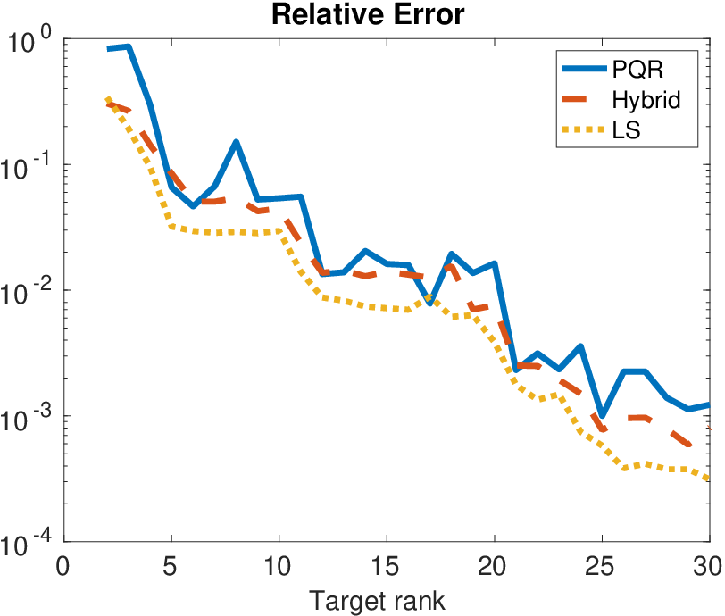


In fig. 5, we compare the error in the DEIM approximations and the corresponding error constants for the various algorithms. The error constant is much smaller for the LS point selection algorithm compared to both the hybrid and deterministic approaches. This is because the number of samples in the LS point selection algorithm is much larger than . However, the accuracy of the DEIM approximation is comparable for all three methods, and does not appear to be significantly affected by the choice of the point selection method. The computational time for each point selection method is also reported, the timings were averaged over runs.


To provide more insight into the hybrid point selection algorithm, we compare it with sRRQR and LS point selection algorithms. In fig. 6, we plot the point selected by the LS sampling approach on the left panel. By construction, the hybrid approach subsamples from the points selected by the LS algorithm, and these points are overlaid in the figure. In the right panel of the same figure, the hybrid points are compared with those selected by sRRQR. It it interesting to note that several points overlap between the hybrid and the sRRQR approaches, even though they were selected using different algorithms.
Our conclusion is that the proposed hybrid point selection algorithm is a good compromise between the deterministic (e.g., PQR, sRRQR) and randomized point selection algorithms. Compared to the deterministic algorithms it is computationally efficient and has comparable accuracy. The hybrid point selection algorithm also has comparable accuracy to the LS algorithm but is advantageous since only components of the nonlinear function need to be evaluated.
6.3 Example 3: PDE-based application
We consider a example from [25, section 8.4] involving a parameterized advection-diffusion PDE that models, for example, the evolution of the concentration of a pollutant. Consider the following PDE defined on a domain with boundary
| (18) | |||||
| (19) |
Here, , is a positive constant, and is the normal vector. The wind velocity is taken to be , which is a constant in space but depends nonlinearly on the parameter . The source term has the form of a Gaussian function centered at and spread , i.e.,
The cost of solving the PDE for many different values of is high and therefore, it is computationally beneficial to develop a reduced order model that makes the online solution of the PDE feasible. The nonlinear dependence on the parameters arises from the source term . To tackle this, we use the POD-DEIM approach.


Our first experiment is similar to that in [25, section 10.5.1]. We first consider the cost of approximating the source term over the range of parameters , and is chosen between . A training set for is generated by Latin hypercube sampling with training points. Two different approximations are generated using DEIM and R-DEIM. The number of DEIM basis vectors used were and was determined based on the singular value decay of the snapshot matrix. The R-DEIM basis is also fixed to be of size and was computed using algorithm 1 with an oversampling parameter . The error is computed by averaging over different randomly generated test points. The results are displayed in fig. 7. The hybrid point selection algorithm is used for both the standard DEIM basis and the randomized DEIM basis—the same parameters are used as in section 6.2. As can be seen the error between the two different methods are comparable. For this application, the number of quadrature nodes is . It is worth mentioning that the CPU time for computing the compact SVD is seconds whereas the CPU time for the randomized range finder is seconds. The computational time for the point selection was comparatively seconds. The speedup is more impressive for larger problems; see [2] for more detailed comparisons on large-scale problems.
Our second experiment is similar to [25, section 10.5.2], in which the parameters and are fixed and the remaining parameters are taken to be in the range , and . The goal is then to compute a ROM for solving the PDE eq. 17 for the above chosen range of parameters. The source term is approximated using the DEIM and the R-DEIM approaches, as described in the previous experiment (the dimension was used for both approximations. The POD algorithm is computed using snapshots and the POD dimension is used to construct the reduced basis space. The error is shown in the right panel of fig. 7, where the POD-R-DEIM approximation is compared against the POD-DEIM approximation. It is seen that both the errors are comparable which validates our approach.
7 Conclusions
We have provided randomized algorithms for tackling the two main bottlenecks of the standard DEIM algorithm. First, we propose several randomized algorithms for approximately computing the DEIM basis and highlight various benefits of the randomized algorithms including adaptivity. Second, we proposed two randomized point selection algorithms— one based on leverage score sampling, the other combines leverage score and rank-revealing factorizations. We provide detailed analysis of the error in the resulting algorithms that clearly show the trade-off between computational cost and accuracy. The proposed algorithms are more efficient than the standard techniques and have comparable accuracy. Numerical experiments in section 6 confirm these findings and give insight into the choice of parameters.
8 Acknowledgments
The author would like to thank Ilse C.F. Ipsen and Zlatko Drmač for discussions and Ivy Huang for her help with this manuscript.
References
- [1] S. S. Aslan, E. de Sturler, and M. E. Kilmer. Randomized approach to nonlinear inversion combining simultaneous random and optimized sources and detectors. arXiv preprint arXiv:1706.05586, 2017.
- [2] C. Bach, F. Duddeck, and L. Song. Fixed-precision randomized low-rank approximation methods for nonlinear model order reduction of large systems. International Journal for Numerical Methods in Engineering, 119(8):687–711, 2019.
- [3] P. Benner, S. Gugercin, and K. Willcox. A survey of projection-based model reduction methods for parametric dynamical systems. SIAM review, 57(4):483–531, 2015.
- [4] D. A. Bistrian and I. M. Navon. Randomized dynamic mode decomposition for nonintrusive reduced order modelling. International Journal for Numerical Methods in Engineering, 112(1):3–25, 2017.
- [5] C. Boutsidis, M. W. Mahoney, and P. Drineas. An improved approximation algorithm for the column subset selection problem. In Proceedings of the twentieth annual ACM-SIAM symposium on Discrete algorithms, pages 968–977. SIAM, 2009.
- [6] M. E. Broadbent, M. Brown, K. Penner, I. C. Ipsen, and R. Rehman. Subset selection algorithms: Randomized vs. deterministic. SIAM Undergraduate Research Online, 3:50–71, 2010.
- [7] S. Chaturantabut and D. C. Sorensen. Nonlinear model reduction via discrete empirical interpolation. SIAM Journal on Scientific Computing, 32(5):2737–2764, 2010.
- [8] P. Drineas and M. W. Mahoney. RandNLA: randomized numerical linear algebra. Communications of the ACM, 59(6):80–90, 2016.
- [9] Z. Drmač and S. Gugercin. A new selection operator for the discrete empirical interpolation method—improved a priori error bound and extensions. SIAM Journal on Scientific Computing, 38(2):A631–A648, 2016.
- [10] Z. Drmač and A. K. Saibaba. The discrete empirical interpolation method: Canonical structure and formulation in weighted inner product spaces. SIAM Journal on Matrix Analysis and Applications, 39(3):1152–1180, 2018.
- [11] N. B. Erichson, S. L. Brunton, and J. N. Kutz. Randomized dynamic mode decomposition. arXiv preprint arXiv:1702.02912, 2017.
- [12] N. B. Erichson and C. Donovan. Randomized low-rank dynamic mode decomposition for motion detection. Computer Vision and Image Understanding, 146:40–50, 2016.
- [13] C. Gorman, G. Chávez, P. Ghysels, F.-H. Rouet, and X. S. Li. Matrix-free construction of HSS representation using adaptive randomized sampling. arXiv preprint arXiv:1810.04125, 2018.
- [14] M. Gu. Subspace iteration randomization and singular value problems. SIAM Journal on Scientific Computing, 37(3):A1139–A1173, 2015.
- [15] M. Gu and S. C. Eisenstat. Efficient algorithms for computing a strong rank-revealing QR factorization. SIAM Journal on Scientific Computing, 17(4):848–869, 1996.
- [16] N. Halko, P. G. Martinsson, and J. A. Tropp. Finding structure with randomness: Probabilistic algorithms for constructing approximate matrix decompositions. SIAM review, 53(2):217–288, 2011.
- [17] J. S. Hesthaven, G. Rozza, and B. Stamm. Certified reduced basis methods for parametrized partial differential equations. Springer, 2016.
- [18] J. T. Holodnak and I. C. Ipsen. Randomized approximation of the Gram matrix: Exact computation and probabilistic bounds. SIAM Journal on Matrix Analysis and Applications, 36(1):110–137, 2015.
- [19] I. C. F. Ipsen and T. Wentworth. The effect of coherence on sampling from matrices with orthonormal columns, and preconditioned least squares problems. SIAM Journal on Matrix Analysis and Applications, 35(4):1490–1520, 2014.
- [20] M. W. Mahoney et al. Randomized algorithms for matrices and data. Foundations and Trends® in Machine Learning, 3(2):123–224, 2011.
- [21] P. G. Martinsson and S. Voronin. A randomized blocked algorithm for efficiently computing rank-revealing factorizations of matrices. SIAM Journal on Scientific Computing, 38(5):S485–S507, 2016.
- [22] B. Peherstorfer, D. Butnaru, K. Willcox, and H. J. Bungartz. Localized discrete empirical interpolation method. SIAM Journal on Scientific Computing, 36(1):A168–A192, 2014.
- [23] B. Peherstorfer, Z. Drmač, and S. Gugercin. Stabilizing discrete empirical interpolation via randomized and deterministic oversampling. arXiv preprint arXiv:1808.10473, 2018.
- [24] B. Peherstorfer and K. Willcox. Online adaptive model reduction for nonlinear systems via low-rank updates. SIAM Journal on Scientific Computing, 37(4):A2123–A2150, 2015.
- [25] A. Quarteroni, A. Manzoni, and F. Negri. Reduced basis methods for partial differential equations: an introduction, volume 92. Springer, 2015.
- [26] Y. Saad. Numerical Methods for Large Eigenvalue Problems: Revised Edition. SIAM, 2011.
- [27] A. K. Saibaba. Randomized subspace iteration: Analysis of canonical angles and unitarily invariant norms. SIAM Journal on Matrix Analysis and Applications, 40(1):23–48, 2019.
- [28] D. C. Sorensen and M. Embree. A DEIM induced CUR factorization. SIAM Journal on Scientific Computing, 38(3):A1454–A1482, 2016.
- [29] G. W. Stewart and J.-G. Sun. Matrix perturbation theory. Computer Science and Scientific Computing. Academic Press, Inc., Boston, MA, 1990.
- [30] D. B. Szyld. The many proofs of an identity on the norm of oblique projections. Numerical Algorithms, 42(3):309–323, 2006.
- [31] J. A. Tropp, A. Yurtsever, M. Udell, and V. Cevher. Practical sketching algorithms for low-rank matrix approximation. SIAM Journal on Matrix Analysis and Applications, 38(4):1454–1485, 2017.
- [32] P. Å. Wedin. On angles between subspaces of a finite dimensional inner product space. In Matrix Pencils, pages 263–285. Springer, 1983.
- [33] D. Yu and S. Chakravorty. A randomized proper orthogonal decomposition technique. In American Control Conference (ACC), 2015, pages 1137–1142. IEEE, 2015.
- [34] D. Yu and S. Chakravorty. A computationally optimal randomized proper orthogonal decomposition technique. In American Control Conference (ACC), 2016, pages 3310–3315. IEEE, 2016.
- [35] W. Yu, Y. Gu, and Y. Li. Efficient randomized algorithms for the fixed-precision low-rank matrix approximation. SIAM Journal on Matrix Analysis and Applications, 39(3):1339–1359, 2018.