Non-Kitaev spin liquids in Kitaev materials
Abstract
We point out that the Kitaev materials may not necessarily support Kitaev spin liquid. It is well-known that having a Kitaev term in the spin interaction is not the sufficient condition for the Kitaev spin liquid ground state. Many other spin liquids may be stabilized by the competing spin interactions of the systems. We thus explore the possibilities of non-Kitaev spin liquids in the honeycomb Kitaev materials. We carry out a systematic classification of gapped spin liquids using the Schwinger boson representation for the spin variables. The presence of strong spin-orbit coupling in the Kitaev materials brings new ingredients into the projective symmetry group classification of the non-Kitaev spin liquid. We predict the spectroscopic properties of these gapped non-Kitaev spin liquids. Moreover, among the gapped spin liquids that we discover, we identify the spin liquid whose spinon condensation leads to the zig-zag magnetic order that was observed in Na2IrO3 and -RuCl3. We further discuss the possibility of gapped spin liquid and the deconfined quantum criticality from the zig-zag magnetic order to spin dimerization in pressurized -RuCl3.
I Introduction
Kitaev spin liquid was proposed by A. Kitaev when he constructed an elegant model and solved it exactly Kitaev 2006. An interesting connection to Na2IrO3 was made by G. Jackeli and G. Khaliulin Jackeli and Khaliullin 2009. It was shown that the strong spin-orbit coupling (SOC) of iridium electrons could give rise to a Kitaev interaction in the effective spin Hamiltonian for the iridium local moments. Since then, many iridates were synthesized and explored Kitagawa et al. 2018; Terzic et al. 2015; Comin et al. 2012; Sohn et al. 2013; Ye et al. 2012; Gretarsson et al. 2013a; Gretarsson et al. 2013b; Liu et al. 2011; Takayama et al. 2015; Modic et al. 2014, including the recent -RuCl3 Binotto et al. 1971; Pollini 1996; Plumb et al. 2014; Sandilands et al. 2016; Banerjee et al. 2016; Banerjee et al. 2017 and the very early hyperkagome lattice spin liquid material Na4Ir3O8 Okamoto et al. 2007 where the local moment Kim et al. 2008 and the anisotropic spin interaction were proposed Chen and Balents 2008. These materials are dubbed “Kitaev materials” and have sparked an active search of Kitaev spin liquid Trebst 2017; Zhou et al. 2017; Knolle and Moessner 2018; Hermanns et al. 2018; Savary and Balents 2017.
Generally speaking, the list of Kitaev materials goes beyond iridates and ruthenates Li et al. 2017a; Rau and Gingras 2018; Jang et al. 2018. What gives the Kitaev interaction is the strong SOC, and this is common to magnetic materials with heavy atoms. Therefore, any strong spin-orbit-coupled Mott insulator with spin-orbit-entangled effective spin-1/2 moments and a proper lattice geometry can be a Kitaev material. In particular, the rare-earth magnets, that have the same lattice structure as iridates and ruthenates, could be ideal Kitaev materials Li et al. 2017a. Despite the growing list of Kitaev materials, all these systems face one crucial issue—there are many competing interactions that coexist with the Kitaev interaction. For example, for the nearest-neighbor bonds in Na2IrO3 and -RuCl3, three extra interactions beyond the Kitaev interaction are present Rau et al. 2014, not to mention many further neighbor (anisotropic) spin interactions that arise from the large spatial extension of the / electron wavefunction.
In fact it has been shown that Kitaev spin liquid is fragile and small perturbation could actually destabilze it Jiang et al. 2011; Chaloupka et al. 2013; Nasu et al. 2017; Rousochatzakis et al. 2015; Sizyuk et al. 2014. Meanwhile, the real materials contain many competing interactions that may be as important as the Kitaev interaction, the candidate quantum spin liquids (QSLs) for these materials remain to be examined. On the other hand, for any other gapped QSL that is not Kitaev spin liquid, if it is realized, it will be stable against small local perturbations regardless of the Kitaev interaction. This means that having the Kitaev interaction in the Hamiltonian is insufficient to induce Kitaev spin liquid and other competing interactions could instead favor different QSL ground states. For example, the - spin-1/2 Heisenberg model on the honeycomb lattice in certain parameter regime was proposed to support a gapped QSL that is clearly not a Kitaev spin liquid Gong et al. 2013.
In this work, we deviate from the “hot spot” of searching for Kitaev spin liquid in Kitaev materials. Instead, our goal here is to find possible candidate QSLs in Kitaev materials that are not Kitaev spin liquid and to predict the experimental consequences of them. Considering the richness of Kitaev materials, it is very likely that these non-Kitaev QSLs may actually be stabilized in certain systems. A recent study of pressurized -RuCl3 indeed suggested some evidence for a possible QSL Wang et al. 2018. This experimental work motivates us to search for non-Kitaev QSLs in these systems. We carry out a systematic projective symmetry group (PSG) classification of gapped QSLs on a honeycomb lattice using Schwinger boson Read and Sachdev 1991; Wen 2002a; Wen 2002b; Wang and Vishwanath 2006; Wang 2010 representation of the spins. Due to the spin-orbit-entangled nature of the local moments, the symmetry transformation operates both on the spin components and on the spin position Li et al. 2017b; Reuther et al. 2014; Schaffer et al. 2013. This new symmetry property gives a different classification scheme from the existing PSG analysis. From the PSG results, we predict the spectroscopic properties of different QSLs on the honeycomb lattice. Moreover, we study the proximate magnetic orders out of the QSLs by condensing the spinons Read and Sachdev 1991; Sachdev 1992. The magnetic wavevector of the zig-zag magnetic order, that was observed in Na2IrO3 and -RuCl3 Ye et al. 2012; Chaloupka et al. 2013; Sears et al. 2015, naturally connects with the 2B QSLs via the spinon condensation.
The remaining parts of the paper are organized as follows. In Sec. II, we introduce the Schwinger boson construction for the QSLs with spin-orbit-entangled local moments. In Sec. III, we explain the specific properties of the symmetry operations under the Schwinger boson framework. In Sec. IV, we obtain 16 distinct QSLs from the PSG classifications and study the phase diagram of several representative mean-field QSL states. In Sec. V, we explore the spectroscopic properties and the proximate magnetic phases of the aforementioned mean-field QSLs. Finally in Sec. VI, we discuss the relevant experiments and especially explain the possibilities for the pressurized -RuCl3.
II Schwinger boson construction
The gapped spin liquids can be studied by either Schwinger boson or Abrikosov fermion approach. We here adopt the Schwinger boson construction since it is easier to explore the proximate magnetic orders with bosonic variables. In the Schwinger boson representation, the effective spin on site is given by where () is the bosonic spinon operator. The Hilbert space is enlarged due to the introduction of the spinons; to project out unphysical states, the constraint on local boson number is imposed. The most general candidate mean-field Hamiltonian for the spin liquids has the following form,
| (1) | |||||
where we have restricted the mean-field ansatz to nearest neighbors and introduced the chemical potential to enforce the boson number constraint and we have used the superscript A/B to represent hopping/pairing terms in the coefficients . Due to the spin-orbit-entangled nature of the local moments, the SU(2) symmetry breaking terms exist in the mean-field ansatz. Using the hermiticity of the Hamiltonian and bosonic statistics of the spinons, it is easy to show that , , , and .

III Projective symmetry group
In this section we follow the projective symmetry group (PSG) approach introduced in Refs. Wen 2002a; Wen 2002b to classify the spinon mean field states based on the symmetries of the honeycomb layers of Kitaev materials. The spinon mean field state will be a reasonable description of the QSLs, provided the QSL survives the quantum fluctuations beyond mean field.
The physical symmetry group of the Hamiltonian contains both space group symmetries and the time-reversal symmetry. For simplicity, we fix the representation of the time-reversal symmetry to be the following throughout the paper:
| (2) |
The space group symmetries, on the other hand, can be represented projectively by the spinons. Therefore, we will only take the space group symmetries into account for the PSG classification; the time-reversal symmetry commutes with all the space group symmetries and does not affect the classification (see Appendix B). The time-reversal symmetry will nevertheless restrict the form of the mean-field Hamiltonian (see Appendix C).
The lattice system of the honeycomb layer is shown in Fig. 1 and defined in Appendix A. The space group is generated by two translations and , a counterclockwise sixfold rotation around the hexagon center, and a reflection around the horizontal axis through the same hexagon center. Under the symmetry operation , the bosonic spinon transforms as
| (3) |
where is a local U(1) gauge transformation, which leaves the spin operators invariant. The gauge transformation is generally nontrivial, hence incorporated in the symmetry operation in Eq. (3). After projection into the physical Hilbert space, spinons states related by a pure gauge transformation should give the same physical state. In Eq. (3) we have introduced the spin rotation to account for the effects of SOC, which rotates the position and spin simultaneously. In explicit forms, we have .
For mean-field Hamiltonian of the form in Eq. (1) to be invariant under the symmetry transformation , the coefficients should satisfy
| (4) | |||||
| (5) |
where we have used the fact that commutes with . For a general pair of sites , the above equations are solvable if for each group relation , the following identities are satisfied,
| (6) |
where is either element of , the invariant gauge group (IGG). The IGG turns out to be the gauge group of the low-energy effective theory of the QSL state Wen 2002a; Wen 2002b. Here, since we are considering QSLs, the IGG should also be . The two lines in Eq. (III) are equivalent because the identity element involves either rotation by or , so , and the group relations constraint only the phases . Given the defining relations between group generators , we can solve for all the possible gauge transformation functions ’s compatible with Eq. (III).
| QSL | |||||
|---|---|---|---|---|---|
| 2A000 | |||||
| 2A001 | |||||
| 2A010 | |||||
| 2A011 | |||||
| 2A100 | |||||
| 2A101 | |||||
| 2A110 | |||||
| 2A111 | |||||
| 2B000 | |||||
| 2B001 | |||||
| 2B010 | |||||
| 2B011 | |||||
| 2B100 | |||||
| 2B101 | |||||
| 2B110 | |||||
| 2B111 |
IV The 16 classes of QSLs and the mean-field phase diagram
The solutions of the ’s for equations of the form in Eq. (III) are as follows:
| (7) | |||
| (8) | |||
| (9) | |||
| (10) | |||
| (11) |
where and are free to take either or in . Details of the derivation can be found in Appendix B. Therefore there are in total 16 states labeled by and . Specifically, the state is called 2A states when , and 2B states when . This variable is proportional to the magnetic flux through each unit cell felt by the spinon. It signifies the fractionalization of translation symmetry to be discussed in Sec. V.
With the PSG solutions in Tab. 1, we obtain the mean-field Hamiltonians for Schwinger bosons in Appendix C. The simplified results are summarized in Tab. 2. Due to constraints from the PSG, the hermiticity of the Hamiltonian, and time-reversal symmetry, some of the coefficients are fixed to be .
| QSL | ||||
|---|---|---|---|---|
| 2A000 | ||||
| 2A001 | ||||
| 2A010 | ||||
| 2A011 | ||||
| 2A100 | ||||
| 2A101 | ||||
| 2A110 | ||||
| 2A111 | ||||
| 2B000 | ||||
| 2B001 | ||||
| 2B010 | ||||
| 2B011 | ||||
| 2B100 | ||||
| 2B101 | ||||
| 2B110 | ||||
| 2B111 |


The classification of QSLs incorporate a wide range of phases (at least one for each class) and encode different types of interactions. This is particularly relevant to Kitaev materials, where interactions beyond the Kitaev model compete with the Kitaev term. These interactions can drive the system away from the Kitaev spin liquid state into other QSLs, or even destablize the spin liquid and introduce a magnetic order. It is therefore desirable to investigate the phase diagram for the QSL states in our classification and determine the ranges of the parameters that support a QSL phase. We can further predict their proximate magnetic orders that can be directly compared with experiments.
The magnetic order out of the QSLs can be understood in the following manner. In the QSL phases, the spinons are fully gapped, and the system are absent from developing long-range order. However, as we have mentioned in Sec. II, the spinon density must satisfy the uniform filling condition
| (12) |
Such a constraint is met by tuning the chemical potential within the mean field theory. At a critical value of , the spinon gap will close and the spinons condense at the band miminum with . It will correspondingly give rise to a magnetic order or spin density wave with ordering wavevector (see Sec. V.2).
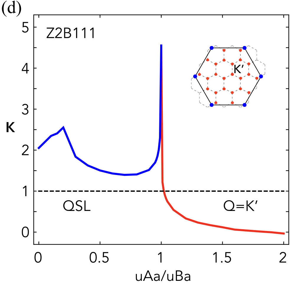
Here we choose four representative classes, 2A100, 2A111, 2B100, 2B111, and solve for their mean-field phase diagrams (see Fig. 2). We found that the 2A111, 2B100, 2B111 states all support paramagnetic QSL phases in the chosen parameter regime, and all of these QSL states can be driven to magnetic order when certain parameters are tuned.
V Experimental consequences of QSLs
In this section we discuss two experimental consequences of the QSLs. First, we note that translation symmetry fractionalization in 2B states will result in an enhanced periodicity of the lower edge of the dynamic spin structure factor, which serves as a direct spectroscopic probe for the QSLs. Second, we study magnetic ordered states adjacent to QSLs via the condensation of Schwinger bosons. It turns out that the ordering nature of the boson-condensed state are determined by the classes of QSLs. Therefore the experimentally measured magnetic ordered states will impose restrictions on possible adjacent QSLs, which helps determine the nature of the experimentally realized spin liquids.
V.1 Spectroscopic signatures of translational symmetry fractionalization
A unique feature of QSLs is the emergent fractionalized excitations; in our case, these are the gapped spinons or visons. The spinons carry quantum numbers that are fractions of a physical spin. This fact prevents spinons from being directly probed, since any local observable is necessarily with integer quantum number, and the observable necessarily adopts a “convoluted” form in terms of spinon variables. In inelastic neutron scattering experiments, one neutron flip event creates a spin-1 excitation, and the energy-transfer of the neutron is shared between a pair of spin-1/2 spinons,
| (13) | |||||
| (14) |
In the previous section we classified gapped QSLs on the honeycomb lattice, each characterized by a projective representation the emergent spinons live in. It was realized that the symmetry class of spinons has dramatic effects on the neutron spectrum Essin and Hermele 2013; Essin and Hermele 2014. For the lattice translation, the relevant quantum number is , and we find
| (15) | |||||
| (16) |
For the 2B states, , and the PSG elements corresponding to and anticommute,
| (17) |
where and act on the spinon degrees of freedom instead on the spins. As a consequence, the periodicity of the lower excitation edge of the dynamic spin structure factor defined by
| (18) |
is doubled (see Appendix C),
For the 2A states, the lower excitation edge should have the usual periodicity of in both directions of Brillouin zone basis.
We illustrate the two possible fractionalization patterns in Fig. 3 representative 2A and 2B states. This pattern is accessible to neutron scattering experiments.


V.2 Proximate magnetic orders of QSLs
Besides the symmetry fractionalization in the QSL phases, the proximate magnetic orders in the spinon-condensed phases provide a complementary description of the system. Instead of two-spinon continuum, one expects to see sharp magnon peaks in the neutron or the resonant inelastic X-ray scattering data. Therefore, the enhanced spectral periodicity in the previous section is no longer a relevant description; it is much more feasible to directly probe the magnetic order. It would make a strong case for the QSL parent state if some of the magnetic orders depicted in Fig. 2 are observed.
In fact, we show here that the proximate magnetic order of the 2B100 state (see Fig. 2c) has the same ordering wave vector as the zig-zag order with ordering wave vector observed in Kitaev materials -RuCl3 and Na2IrO3.
The mean-field Hamiltonian Eq. (1) of a typical 2B state in momentum space reads
| (19) |
where
| (20) |
and labels the and sublattices of the honeycomb lattice, labels the spin indices, and labels the sites in each magnetic unit cell (due to the -flux in each of the original unit cell). The spectrum has an enhanced periodicity as expected.


As we see from Fig. 2c, in a large range of parameters the high symmetry points are the two independent minimum of the spinon band structure in the magnetic Brillouin zone for the 2B100 state. Moreover, the spinons condense at band minima in that regime, and the system is magnetically ordered. The corresponding spinon condensate has the following form:
| (21) |
where and are eigenvectors of at with the lowest energy, respectively.
The choices of the coefficient ’s are subject to following constraints:
1) The condition for all fixes with respect to ;
2) The boson density should be uniform across the lattice system. This condition will fix .
With the condensate, it is ready to calculate the magnetic order with
| (22) |
We see immediately that the magnetic order has an ordering wave vector of , consistent with the experimentally observed magnetic Bragg peak, and the magnetic order is controlled by two real parameters while the overall phase factor is inessential. We have a limited set of free parameters for the magnetic order, so the magnetic order would take a rather fixed pattern, as illustrated in Fig. 4. As the zig-zag order, the ordering pattern is periodic in the chain direction and antiferromagnetic between the neighboring chains.
Although the order differs from the zig-zag or stripe ones, we suspect that this is an artifact of the spinon mean-field theory approach. In this framework, we are effectively dealing with a theory of free spinons with only nearest neighbor hopping. We expect that when further neighbor hoppings and interlayer interactions are taken into account, the magnetic order should be closer to reality. On the other hand, the -flux is a robust feature and will survive interactions. Consequently, the ordering wave vector will exist for a large range of parameters.
To further constrast the 2B states with the 2A states, we note that the proximate magnetic orders in the phase diagrams of 2A states in Fig. 2 are either incommensurate with the lattice, or have an ordering vector of or . As a consequence, the resulting magnetic order is either ferromagnetic (see Appendix. E) or an antiferromagnetic order. Both are drastically different from the zig-zag order that was observed.
In summary, we have pointed out that the 2B100 state is likely to be the QSL state adjacent to the zig-zag ordered states observed in Kitaev materials -RuCl3 and Na2IrO3.
VI Discussion
The proposed honeycomb lattice Kitaev materials are Li2IrO3, Na2IrO3, and -RuCl3 with magnetic ions. Unfortunately, all three materials develop long-range magnetic orders, and the relevant magnetic orders were proposed to be the zig-zag like with a magnetic unit cell that is twice of the crystal unit cell Sears et al. 2015; Ye et al. 2012; Chaloupka et al. 2013. For -RuCl3 that is under an active study recently, the magnetic field is found to suppress the magnetism and possibly generate a QSL state at intermediate magnetic fields. The thermal Hall measurement has found a non-vanishing thermal Hall effect that seems to be consistent with the prediction from the chiral majorana fermion edge state that is obtained from the Kitaev spin liquid by the magnetic field Kasahara et al. 2018a; Hentrich et al. 2019; Kasahara et al. 2018b. Because of the particular experimental setup in the thermal Hall measurements, Refs. Ye et al. 2018; Vinkler-Aviv and Rosch 2018 carefully considered the effect of the spin-lattice coupling and suggested that the quantization of the thermal Hall effect may survive and can actually be robust even with the spin-lattice coupling. These results may explain the thermal Hall effect in -RuCl3. In contrast, our result in this paper is not dealing with the actual spin state in the intermediate magnetic fields. Instead, we are interested in the zero-field magnetic state and try to understand whether the magnetic orders can be thought as the proximate magnetic orders of the nearby QSLs. Thus, an indirect experimental signature would be a possible quantum phase transition from the current magnetic orders to the nearly QSLs. It is not obvious if this transition can be induced by the external magnetic field. It is, however, possible that the magnetic field induces the magnetic order from the QSLs via the spinon condensation where the magnetic field suppresses the spinon band gap.
On the other hand, a recent theoretical development Ghioldi et al. 2018 has extended the Schwinger boson construction to understand the dynamical properties of the magnetically ordered state that is obtained by condensing the bosonic spinons. Ref. Ghioldi et al. 2018 applies this theory to study the dynamical properties of the triangular lattice Heisenberg model, despite this model supports the well-known 120-degree magnetic order. Their results suggested that the Schwinger boson approach can be an adequate starting point for describing the excitation spectrum of some magnetically ordered compounds that are near the quantum melting point separating this ordered phase from the proximate QSL. In -RuCl3, the ordered moment is only about 1/3 of the full magnetic moment in the paramagnetic phase Banerjee et al. 2017. Thus, it is natural and interesting to see whether Ref. Ghioldi et al. 2018’s approach can be adapted to provide a new understanding of the spin dynamics inside the magnetic ordered state of -RuCl3 rather than making connection to the Kitaev spin liquid.
Quite recently, the pressurized -RuCl3 has been studied experimentally Wang et al. 2018, as well as other strain effect experiments have been performed. We focus our discussion on the pressurized experiments Wang et al. 2018. It is found that, above a critical pressure, the antiferromagnetic order in -RuCl3 disappears and a possible QSL state appears. At even higher pressures, the system experiences a resistance drop by several orders in magnitude. This was interpreted as the softening or the closing of the charge gap. At the mean time, the magnetoresistivity in this range of pressure remain insensitive to the magnetic field up to 7T. There are several puzzles associated with this pressurized experiment. What is the nature of the disordered state when the magnetic order diappears? What is the nature of the disordered state with a significantly reduced resistance in the high pressure regime? What do the spin degrees of freedom do in this high pressure regime? The experimental information is quite limited to address these questions. However, here we would like make a bold suggestion. First, we discuss the possibility that the disordered state can be a QSL state. The absence of the phase transition in the heat capacity measurement down to 4K suggests that the candidate QSL cannot be a symmetry broken state such as the time reversal symmetry broken chiral spin liquid. From the robustness of a phase in a large range of pressures, the candidate state may be a QSL, and this topological order would survive even to the pressure when the charge gap is suppressed. In fact, Ref. Wang et al. 2018 has attributed the insensitivity of the magnetoresistance to the magnetic field to the dominance of the spin energy scale. In the future experiments, it will be interesting to perform an inelastic neutron scattering measurement to check if the spinon continuum shows a spectral periodicity enhancement. In addition, doping the pressurized materials and examining the possibility of superconductivity or non-Fermi liquid behaviors can be quite interesting too. It is interesting to notice that doping the spin-orbit-coupled Mott insulators such as RuCl3, iridates, or any others with spin-orbit-entangled local moments beyond the moments would necessarily experience an electron-hole doping asymmetry. This doping asymmetry arises from the distinct spin-orbital reconstruction/entanglement of the different electron occupation configurations from electron and hole doping. We will elaborate this general point in a later paper. Furthermore, if the pressurized sample develops a dimerized state, a natural question would be the nature of the phase transtion between the zig-zag magnetic order and the dimerization. Could this transition be a deconfined quantum criticality that is very much like the Néel-VBS transition proposed for the square lattice antiferromagnets Senthil et al.? As the pressure can be tuned continuously, this question could be addressed experimentally by tuning the pressure to the transition point in the future. The other question would be whether the dimerized state can be obtained by condensing visons from the same QSL that gives the zig-zag magnetic order. These two questions can be pushed forward when more experimental results are available.
To summarize, in this paper we have carefully classified the possible QSLs and studied the experimental signatures such as the proximate magnetic orders, symmetry fractionalization of the spinons, and the structure of the spinon continuum. Our results provide a rather different perspective from the existing thoughts on these Kitaev materials.
VII Acknowledgments
We thank Dr. Jiawei Mei and Dr. Khaliullin for telling us the possibility of spin dimerization in the pressurized sample. This work is supported by the ministry of science and technology of China with Grant No.2016YFA0301001, 2016YFA0300500, 2018YFGH000095.
Appendix A The coordinate system and space group
The honeycomb lattice is illustrated in Fig. 1 of the main text. We choose the basis vectors to be
| (23) |
The lattice sites are labeled by , where is the sublattice index. The position of the site is
| (24) |
All momenta vectors are represented in the basis, where
| (25) |
so that . Therefore, the basis vectors of the Brillouin zone has the following forms,
| (26) |
and
| (27) | |||||
| (28) | |||||
| (29) |
We define additional high-symmetry points in the Brillouin zone,
| (30) |
where . corresponds to those with , and those with . Finally,
| (31) |
The symmetry group of the honeycomb lattice consists of translations , a six-fold rotation and a reflection . Explicitly in terms of the lattice indices, their actions read
| (32) | |||||
| (33) | |||||
| (34) | |||||
| (35) |
Appendix B Algebraic solution of the PSG on honeycomb lattice
In this appendix we show classification of algebraic QSLs by solving the PSG defined in Sec. III.
The space group of the honeycomb lattice and its elements are defined in Sec. III. Presentations of the space group are
| (36) |
We will assume the IGG is (see Sec. III), and assume the generator of the IGG is
| (37) |
Elements of the IGG obviously preserves all mean field ansatz; therefore, the classification of algebraic spin liquid states are determined up to an IGG element.
For each space group element , we associate a U(1) phase such that the mean field Hamiltonian is invariant under the combined PSG operation,
| (38) |
The matrices accounts for the effects of SOC (see their definitions in Sec. III).
Before solving for the PSG, we consider the effect of a pure gauge transformation on the U(1) phases associated to each group element. The symmetry operation on the gauge transformed boson reads . Since commutes with , , and , cancel on both sides. Therefore shoud be replaced by , or Wang and Vishwanath 2006
| (39) |
Using the gauge freedom one can always assume (open boundary condition)
| (40) |
For the honeycomb lattice, this can be achieved by solving equations
| (41) | |||
| (42) |
For simplicity of notations we define and .
The identity translates into the following equation of PSG elements,
where the RHS is an element of the IGG. In terms of phases,
| (44) |
where , and we have adopted assumption in Eq. (40). Again from Eq. (40), we see that
| (45) |
In other words, the flux in one elementary hexagon is .
Similarly, from we have
| (46) | |||
| (47) |
The ’s cancel, and the solution for the U(1) phases is
| (48) | |||||
| (49) |
Performing pure gauge transformations, we may further assume Wang 2010
| (50) |
The solution for reads
| (51) | |||||
In the PSG formulation of the group relation , the ’s again cancel. Thus we have
| (52) | |||||
| (53) |
The solution for is
| (54) | |||||
From we have
| (55) |
since acts only on the spin indices and commutes with and . Since , the above equation simplifies to , giving
| (56) |
For we have
| (57) | |||||
where commutes with the rest, and . This results in the constraint
| (58) |
We see immediately by comparing and in this equation.
Summarizing, the solutions of the PSG are
| (65) | |||
| (66) | |||
| (67) | |||
| (68) | |||
| (69) |
where and are free to take either or in . There are in total 16 possible classes of QSLs; the mean field ansatz would further constrain the number of free parameters. The respective gauge transformations for the 16 QSLs are summarized in Tab. 1.
Appendix C Nearest neighbor mean field ansatz of the PSG
| Bond | - | - | - |
|---|---|---|---|
| Bond | - | - | - |
In this appendix we present symmetry allowed mean field ansatz up to nearest neighbors.
The algebraic solution of PSG is very general and usually contains many free parameters. Certain mean field ansatz will put further constraints on the PSG. In particular, if a non-identity space group element transforms a bond to itself or its inverse, the form of exchange terms on this bond will be constrained.
We first consider the spin-flipping pairing terms ( terms). Under the action of ,
| (70) |
Therefore nonzero requires . Under ,
| (71) |
This equation requires .
Similarly we define and . Acting and on the term,
| (72) | |||
| (73) |
From Eq. (73) we immediately conclude that if we require , then , , and .
Applying and on the term, we see that
| (74) | |||
| (75) |
and similarly for . It is obvious that such terms are nonzero only when .
Following the same procedures, we find for terms
| (76) | |||||
| (77) |
and similarly for and .
We construct exchange interactions on all lattice bonds by applying symmetry operations. The results are shown in Tab. 3.
Appendix D Fractionalization of crystal momentum and enhanced periodicity
Defining to be the symmetry group element acting on the spinon sector, we know from previous discussions that
| (78) |
Given a two-spinon product state with total momentum and total energy , the translation operator acts on it by
| (79) |
where . We can construct another three states by translating the second spinon
| (80) | |||||
| (81) | |||||
| (82) |
These states have the same energy as , but with translated momenta,
| (83) | |||||
| (84) | |||||
| (85) |
Therefore, the two-spinon spectrum has an enhanced periodicity if . In particular, the lower edge of
| (86) |
is completely encoded in energies of the two-spinons states with the momentum , thus has the same periodicity,
| (87) | |||||
Otherwise , and the lower excitation edge should have the usual periodicity of in both directions of Brillouin zone basis.
We have shown that commuting and anticommuting single spinon translations gives different spectroscopic features. We now consider presentations of the symmetry group involving translations (since we are ultimately interested in the periodicity in the reciprocal space) on one-spinon sector,
| (88) | |||||
| (89) | |||||
| (90) | |||||
| (91) |
where we followed the convention in Appendix A. Due to the gauge freedom, we can fix and to be , and consistency of the PSG solution requires . With a detailed analysis, we found that Eq. (88), Eq. (89) and Eq. (91) do not give to any obvious type of periodicity, while Eq. (90) gives a fuzzier version of the one constructed by considering translations only. Therefore, considering the whole symmetry group does not introduce more detailed implications of the neutron scattering spectrum.


Rewriting Eq. (88)–(91) in a more convenient form, and taking , , we get
| (92) | |||||
| (93) | |||||
| (94) | |||||
| (95) |
Suppose is a two-spinon product state, we try acting on the second spinon to obtain new eigenstates with the same energy. Then
| (96) | |||||
| (97) | |||||
where are the momenta for individual spinons. The result depends on the single spinon momentum, and does not lead to any obvious extra periodicity.
Similarly, let ,
| (98) | |||||
| (99) | |||||
While the second equation does not tell us much, the first one do carries to with , while we cannot say much about and . This is a fuzzier version of Eq. (87) as it does not carry as much information about the structure of the spectrum.
Appendix E Proximate magnetic order of QSLs
E.1 2A states
Here we briefly comment on the proximate magnetic order resulting from the 2A parent state. In this case, the translation symmetry is not fractionalized, and the proximate magnetic order also preserves such a symmetry. For a large range of parameters, the band minimum is at , giving rise to a ferromagnetic order. The ordering pattern for a typical set of parameters is shown in Fig. 5.
E.2 2B states
In this section we discuss other 2B mean field classes in the PSG classification. Among them the 2B011 class has only one nonzero parameter , and the corresponding ground state is magnetically ordered with ordering wave vector and . Phase diagrams of the other classes are shown in Fig. 6.
We see that for the parameter space we choose, the 2B000 and 2B010 states are always ordered, while 2B001, 2B101, and 2B110 can all support a QSL phase. The ordering wave vector for 2B000 and 2B010 are the same as that of thef 2B100 described and discussed in Sec. III and Sec. IV, and thus consistent with the magnetic Bragg peak at .
References
- Kitaev (2006) A. Kitaev, Annals of Physics 321, 2 (2006).
- Jackeli and Khaliullin (2009) G. Jackeli and G. Khaliullin, Phys. Rev. Lett. 102, 017205 (2009).
- Kitagawa et al. (2018) K. Kitagawa, T. Takayama, Y. Matsumoto, A. Kato, R. Takano, Y. Kishimoto, S. Bette, R. Dinnebier, G. Jackeli, and H. Takagi, Nature 554, 341 (2018).
- Terzic et al. (2015) J. Terzic, J. C. Wang, F. Ye, W. H. Song, S. J. Yuan, S. Aswartham, L. E. DeLong, S. V. Streltsov, D. I. Khomskii, and G. Cao, Phys. Rev. B 91, 235147 (2015).
- Comin et al. (2012) R. Comin, G. Levy, B. Ludbrook, Z.-H. Zhu, C. N. Veenstra, J. A. Rosen, Y. Singh, P. Gegenwart, D. Stricker, J. N. Hancock, D. van der Marel, I. S. Elfimov, and A. Damascelli, Phys. Rev. Lett. 109, 266406 (2012).
- Sohn et al. (2013) C. H. Sohn, H.-S. Kim, T. F. Qi, D. W. Jeong, H. J. Park, H. K. Yoo, H. H. Kim, J.-Y. Kim, T. D. Kang, D.-Y. Cho, G. Cao, J. Yu, S. J. Moon, and T. W. Noh, Phys. Rev. B 88, 085125 (2013).
- Ye et al. (2012) F. Ye, S. Chi, H. Cao, B. C. Chakoumakos, J. A. Fernandez-Baca, R. Custelcean, T. F. Qi, O. B. Korneta, and G. Cao, Phys. Rev. B 85, 180403 (2012).
- Gretarsson et al. (2013a) H. Gretarsson, J. P. Clancy, Y. Singh, P. Gegenwart, J. P. Hill, J. Kim, M. H. Upton, A. H. Said, D. Casa, T. Gog, and Y.-J. Kim, Phys. Rev. B 87, 220407 (2013a).
- Gretarsson et al. (2013b) H. Gretarsson, J. P. Clancy, X. Liu, J. P. Hill, E. Bozin, Y. Singh, S. Manni, P. Gegenwart, J. Kim, A. H. Said, D. Casa, T. Gog, M. H. Upton, H.-S. Kim, J. Yu, V. M. Katukuri, L. Hozoi, J. van den Brink, and Y.-J. Kim, Phys. Rev. Lett. 110, 076402 (2013b).
- Liu et al. (2011) X. Liu, T. Berlijn, W.-G. Yin, W. Ku, A. Tsvelik, Y.-J. Kim, H. Gretarsson, Y. Singh, P. Gegenwart, and J. P. Hill, Phys. Rev. B 83, 220403 (2011).
- Takayama et al. (2015) T. Takayama, A. Kato, R. Dinnebier, J. Nuss, H. Kono, L. S. I. Veiga, G. Fabbris, D. Haskel, and H. Takagi, Phys. Rev. Lett. 114, 077202 (2015).
- Modic et al. (2014) K. A. Modic, T. E. Smidt, I. Kimchi, N. P. Breznay, A. Biffin, S. Choi, R. D. Johnson, R. Coldea, P. Watkins-Curry, G. T. McCandless, J. Y. Chan, F. Gandara, Z. Islam, A. Vishwanath, A. Shekhter, R. D. McDonald, and J. G. Analytis, Nature Communications 5, 4203 (2014).
- Binotto et al. (1971) L. Binotto, I. Pollini, and G. Spinolo, Physica Status Solidi (b) 44, 245 (1971).
- Pollini (1996) I. Pollini, Phys. Rev. B 53, 12769 (1996).
- Plumb et al. (2014) K. W. Plumb, J. P. Clancy, L. J. Sandilands, V. V. Shankar, Y. F. Hu, K. S. Burch, H.-Y. Kee, and Y.-J. Kim, Phys. Rev. B 90, 041112 (2014).
- Sandilands et al. (2016) L. J. Sandilands, Y. Tian, A. A. Reijnders, H.-S. Kim, K. W. Plumb, Y.-J. Kim, H.-Y. Kee, and K. S. Burch, Phys. Rev. B 93, 075144 (2016).
- Banerjee et al. (2016) A. Banerjee, C. Bridges, J.-Q. Yan, A. Aczel, L. Li, M. Stone, G. Granroth, M. Lumsden, Y. Yiu, J. Knolle, et al., Nature materials 15, 733–740 (2016).
- Banerjee et al. (2017) A. Banerjee, J. Yan, J. Knolle, C. A. Bridges, M. B. Stone, M. D. Lumsden, D. G. Mandrus, D. A. Tennant, R. Moessner, and S. E. Nagler, Science 356, 1055 (2017).
- Okamoto et al. (2007) Y. Okamoto, M. Nohara, H. Aruga-Katori, and H. Takagi, Phys. Rev. Lett. 99, 137207 (2007).
- Kim et al. (2008) B. J. Kim, H. Jin, S. J. Moon, J.-Y. Kim, B.-G. Park, C. S. Leem, J. Yu, T. W. Noh, C. Kim, S.-J. Oh, J.-H. Park, V. Durairaj, G. Cao, and E. Rotenberg, Phys. Rev. Lett. 101, 076402 (2008).
- Chen and Balents (2008) G. Chen and L. Balents, Phys. Rev. B 78, 094403 (2008).
- Trebst (2017) S. Trebst, arXiv:1701.07056 (2017).
- Zhou et al. (2017) Y. Zhou, K. Kanoda, and T.-K. Ng, Rev. Mod. Phys. 89, 025003 (2017).
- Knolle and Moessner (2018) J. Knolle and R. Moessner, 1804.02037 (2018).
- Hermanns et al. (2018) M. Hermanns, I. Kimchi, and J. Knolle, Annual Review of Condensed Matter Physics 9, 17 (2018).
- Savary and Balents (2017) L. Savary and L. Balents, Rep. Prog. Phys. 80, 016502 (2017).
- Li et al. (2017a) F.-Y. Li, Y.-D. Li, Y. Yu, A. Paramekanti, and G. Chen, Phys. Rev. B 95, 085132 (2017a).
- Rau and Gingras (2018) J. G. Rau and M. J. P. Gingras, Phys. Rev. B 98, 054408 (2018).
- Jang et al. (2018) S.-H. Jang, R. Sano, Y. Kato, and Y. Motome, arXiv:1807.01443 (2018).
- Rau et al. (2014) J. G. Rau, E. K.-H. Lee, and H.-Y. Kee, Phys. Rev. Lett. 112, 077204 (2014).
- Jiang et al. (2011) H.-C. Jiang, Z.-C. Gu, X.-L. Qi, and S. Trebst, Phys. Rev. B 83, 245104 (2011).
- Chaloupka et al. (2013) J. c. v. Chaloupka, G. Jackeli, and G. Khaliullin, Phys. Rev. Lett. 110, 097204 (2013).
- Nasu et al. (2017) J. Nasu, Y. Kato, J. Yoshitake, Y. Kamiya, and Y. Motome, Phys. Rev. Lett. 118, 137203 (2017).
- Rousochatzakis et al. (2015) I. Rousochatzakis, J. Reuther, R. Thomale, S. Rachel, and N. B. Perkins, Phys. Rev. X 5, 041035 (2015).
- Sizyuk et al. (2014) Y. Sizyuk, C. Price, P. Wölfle, and N. B. Perkins, Phys. Rev. B 90, 155126 (2014).
- Gong et al. (2013) S.-S. Gong, D. N. Sheng, O. I. Motrunich, and M. P. A. Fisher, Phys. Rev. B 88, 165138 (2013).
- Wang et al. (2018) Z. Wang, J. Guo, F. F. Tafti, A. Hegg, S. Sen, V. A. Sidorov, L. Wang, S. Cai, W. Yi, Y. Zhou, H. Wang, S. Zhang, K. Yang, A. Li, X. Li, Y. Li, J. Liu, Y. Shi, W. Ku, Q. Wu, R. J. Cava, and L. Sun, Phys. Rev. B 97, 245149 (2018).
- Read and Sachdev (1991) N. Read and S. Sachdev, Phys. Rev. Lett. 66, 1773 (1991).
- Wen (2002a) X.-G. Wen, Physics Letters A 300, 175 (2002a).
- Wen (2002b) X.-G. Wen, Phys. Rev. B 65, 165113 (2002b).
- Wang and Vishwanath (2006) F. Wang and A. Vishwanath, Phys. Rev. B 74, 174423 (2006).
- Wang (2010) F. Wang, Phys. Rev. B 82, 024419 (2010).
- Li et al. (2017b) Y.-D. Li, Y.-M. Lu, and G. Chen, Phys. Rev. B 96, 054445 (2017b).
- Reuther et al. (2014) J. Reuther, S.-P. Lee, and J. Alicea, Phys. Rev. B 90, 174417 (2014).
- Schaffer et al. (2013) R. Schaffer, S. Bhattacharjee, and Y. B. Kim, Phys. Rev. B 88, 174405 (2013).
- Sachdev (1992) S. Sachdev, Phys. Rev. B 45, 12377 (1992).
- Sears et al. (2015) J. A. Sears, M. Songvilay, K. W. Plumb, J. P. Clancy, Y. Qiu, Y. Zhao, D. Parshall, and Y.-J. Kim, Phys. Rev. B 91, 144420 (2015).
- Essin and Hermele (2013) A. M. Essin and M. Hermele, Phys. Rev. B 87, 104406 (2013).
- Essin and Hermele (2014) A. M. Essin and M. Hermele, Phys. Rev. B 90, 121102 (2014).
- Kasahara et al. (2018a) Y. Kasahara, K. Sugii, T. Ohnishi, M. Shimozawa, M. Yamashita, N. Kurita, H. Tanaka, J. Nasu, Y. Motome, T. Shibauchi, and Y. Matsuda, Phys. Rev. Lett. 120, 217205 (2018a).
- Hentrich et al. (2019) R. Hentrich, M. Roslova, A. Isaeva, T. Doert, W. Brenig, B. Büchner, and C. Hess, Phys. Rev. B 99, 085136 (2019).
- Kasahara et al. (2018b) Y. Kasahara, T. Ohnishi, Y. Mizukami, O. Tanaka, S. Ma, K. Sugii, N. Kurita, H. Tanaka, J. Nasu, Y. Motome, T. Shibauchi, and Y. Matsuda, Nature 559, 227–231 (2018b).
- Ye et al. (2018) M. Ye, G. B. Halász, L. Savary, and L. Balents, Phys. Rev. Lett. 121, 147201 (2018).
- Vinkler-Aviv and Rosch (2018) Y. Vinkler-Aviv and A. Rosch, Phys. Rev. X 8, 031032 (2018).
- Ghioldi et al. (2018) E. A. Ghioldi, M. G. Gonzalez, S.-S. Zhang, Y. Kamiya, L. O. Manuel, A. E. Trumper, and C. D. Batista, Phys. Rev. B 98, 184403 (2018).
- (56) T. Senthil, A. Vishwanath, L. Balents, S. Sachdev, and M. P. A. Fisher, Science 10.1126/science.1091806.