We begin with an overview of CMEs in the context of KELFI. Kernel mean embeddings (KMEs) are an arsenal of techniques used to represent distributions in a RKHS (Muandet et al., 2017). The key object is the mean embedding of a distribution $X\sim\mathbb{P}$ under a positive definite kernel $k$ via $\mu_{X}:=\int_{\mathcal{X}}k(x,\cdot)d\mathbb{P}(x)=\int_{\mathcal{X}}k(x,\cdot)p(x)dx\in\mathcal{H}_{k}$, where the last equality assumes a density $p$ for $\mathbb{P}$ exists and $\mathcal{H}_{k}$ denotes the RKHS of $k$. They encode distributions in the sense that function expectations can be written as $\mathbb{E}[f(X)]=\langle\mu_{X},f\rangle_{\mathcal{H}_{k}}$ if $f\in\mathcal{H}_{k}$. When $\mu_{X}$ can only be estimated empirically in some form denoted as $\hat{\mu}_{X}$, the expectation can be approximated by $\mathbb{E}[f(X)]\approx\langle\hat{\mu}_{X},f\rangle_{\mathcal{H}_{k}}$.

CMEs are KMEs that encode conditional distributions. We specifically focus on their empirical estimates as we assume we only have the resource to obtain $m$ sets of simulation data due to budget constraints. This results in joint samples $\{\bm{\theta}_{j},\mathbf{x}_{j}\}_{j=1}^{m}$ from $p(\mathbf{x}|\bm{\theta})\pi(\bm{\theta})$ by sampling from a proposal prior $\pi$ for $\bm{\theta}_{j}\sim\pi(\bm{\theta})$ and simulating $\mathbf{x}_{j}\sim p(\mathbf{x}|\bm{\theta}_{j})$ at each $\bm{\theta}_{j}$. Note these samples are not necessarily from the original joint distribution $p(\mathbf{x}|\bm{\theta})p(\bm{\theta})$ if $\pi\neq p_{\bm{\Theta}}$.

We define positive definite and characteristic kernels (Sriperumbudur et al., 2010) $k:\mathcal{D}\times\mathcal{D}\to\mathbb{R}$ and $\ell:\vartheta\times\vartheta\to\mathbb{R}$. When relevant, we denote the hyperparameters of $k$ and $\ell$ with $\alpha$ and $\beta$, and refer to them as $k_{\alpha}=k(\cdot,\cdot;\alpha)$ and $\ell_{\beta}=\ell(\cdot,\cdot;\beta)$. An useful example of such a kernel is an anisotropic Gaussian kernel $\ell(\bm{\theta},\bm{\theta}^{\prime};\bm{\beta})=\exp{\big(-\frac{1}{2}\sum_{d=1}^{D}(\theta_{d}-\theta_{d}^{\prime})^{2}/\beta_{d}^{2}\big)}$ whose hyperparameters are length scales $\bm{\beta}=\{\beta_{d}\}_{d=1}^{D}$ for each dimension $d\in[D]:=\{1,\dots,D\}$, and similarly for $k$.

For any function $f\in\mathcal{H}_{k}$, we construct an approximation to $\mathbb{E}[f(\mathbf{X})|\bm{\Theta}=\bm{\theta}]$ by the inner product $\langle f,\hat{\mu}_{\mathbf{X}|\bm{\Theta}=\bm{\theta}}\rangle_{\mathcal{H}_{k}}$ with an empirical CME $\hat{\mu}_{\mathbf{X}|\bm{\Theta}=\bm{\theta}}$. Importantly, $\hat{\mu}_{\mathbf{X}|\bm{\Theta}=\bm{\theta}}$ is estimated from the joint samples $\{\bm{\theta}_{j},\mathbf{x}_{j}\}_{j=1}^{m}$, even though it is encoding the corresponding conditional distribution $p(\mathbf{x}|\bm{\theta})$. This approximation admits the following form (Song et al., 2009),

where $\mathbf{f}:=\{f(\mathbf{x}_{j})\}_{j=1}^{m}$, $L:=\{\ell(\bm{\theta}_{i},\bm{\theta}_{j})\}_{i,j=1}^{m}$, $\bm{\ell}(\bm{\theta}):=\{\ell(\bm{\theta}_{j},\bm{\theta})\}_{j=1}^{m}$, and $\lambda\geq 0$ is a regularization parameter. This approximation is known to converge at $O_{p}(m^{-\frac{1}{4}})$ if $\lambda$ is chosen to decay at $O_{p}(m^{-\frac{1}{2}})$ or better under appropriate assumptions on $p(\mathbf{x}|\bm{\theta})$ (Song et al., 2013).

We begin by presenting our surrogate likelihood model. Since the likelihood (2.1) is an expectation under $p(\mathbf{x}|\bm{\theta})$, we propose to approximate it via an inner product with the CME of $p(\mathbf{x}|\bm{\theta})$. Specifically, if we choose $k$ such that $\kappa_{\epsilon}(\mathbf{y},\cdot)\in\mathcal{H}_{k}$, then $p_{\epsilon}(\mathbf{y}|\bm{\theta})$ can be approximated by $q(\mathbf{y}|\bm{\theta}):=\langle\kappa_{\epsilon}(\mathbf{y},\cdot),\hat{\mu}_{\mathbf{X}|\bm{\Theta}=\bm{\theta}}\rangle_{\mathcal{H}_{k}}$. We refer to $q(\mathbf{y}|\bm{\theta})$ as the kernel means likelihood (KML). While the KML provides an asymptotically correct likelihood surrogate, for finitely many simulations it is not necessarily positive nor normalized. By using $f=\kappa_{\epsilon}(\mathbf{y},\cdot)$ in (3.1) where $\bm{\kappa}_{\epsilon}(\mathbf{y}):=\{\kappa_{\epsilon}(\mathbf{y},\mathbf{x}_{j})\}_{j=1}^{m}$ and $\mathbf{v}(\mathbf{y}):=(L+m\lambda I)^{-1}\bm{\kappa}_{\epsilon}(\mathbf{y})$, the KML becomes

The KML converges at the same rate as the CME. See theorem A.3 for proof. It is worthwhile to note that the assumption $\ell(\bm{\theta},\cdot)\in\mathrm{image}(C_{\bm{\Theta}\bm{\Theta}})$ is common for CMEs, and is not as restrictive as it may first appear, as it can be relaxed through introducing the regularization hyperparameter $\lambda$ (Song et al., 2013).

To satisfy $\kappa_{\epsilon}(\mathbf{y},\cdot)\in\mathcal{H}_{k}$, we choose the standard Gaussian $\epsilon$-kernel $\kappa_{\epsilon}(\mathbf{y},\mathbf{x})=\mathcal{N}(\mathbf{y}|\mathbf{x},\epsilon^{2}I)$ and let $k_{\alpha}=k_{\epsilon}$ be a Gaussian kernel with length scale $\alpha=\epsilon$. Since $\kappa_{\epsilon}(\mathbf{y},\mathbf{x})$ and $k_{\epsilon}(\mathbf{y},\mathbf{x})$ are scalar multiples of each other, we have that $\kappa_{\epsilon}(\mathbf{y},\cdot)\in\mathcal{H}_{k}$. In fact, any positive definite kernel $\kappa_{\epsilon}$ can be used, since we can simply choose $k_{\alpha}$ to be its scalar multiple to form the RKHS.

When the raw data is iid and no sufficient summary statistics are available, we can employ a kernel on the empirical distributions of the two datasets via $\kappa_{\epsilon,\alpha}(\mathbf{y},\mathbf{x})\propto k_{\epsilon,\alpha}(\mathbf{y},\mathbf{x})=\exp{\big(-\frac{1}{2\epsilon^{2}}\|\hat{\mu}_{\mathbf{Y}}-\hat{\mu}_{\mathbf{X}}\|_{\mathcal{H}_{k}}^{2}\big)}$, where $\hat{\mu}_{\mathbf{Y}}=\frac{1}{n}\sum_{i=1}^{n}\bar{k}_{\alpha}(\mathbf{y}_{i},\cdot)$, $\hat{\mu}_{\mathbf{X}}=\frac{1}{n}\sum_{i=1}^{n}\bar{k}_{\alpha}(\mathbf{x}_{i},\cdot)$ are empirical mean embeddings of the observed and simulated raw data. Here $\bar{k}$ is another kernel with hyperparameters $\alpha$. This was also used in double kernel ABC (K2-ABC) (Park et al., 2016) and distribution regression ABC (DR-ABC) (Mitrovic et al., 2016) to remove the requirement of summary statistics.

We now propose a hyperparameter learning algorithm for our surrogate likelihood model. The main advantage of using an approximate surrogate likelihood surrogate model is that it readily provides a marginal surrogate likelihood quantity that lends itself to a hyperparameter learning algorithm. We define the marginal kernel means likelihood (MKML) as follows,

where $\mu_{\bm{\Theta}}:=\int_{\vartheta}\ell(\bm{\theta},\cdot)p(\bm{\theta})d\bm{\theta}$ is the mean embedding of $p_{\bm{\Theta}}$. If we choose $\ell$ to be an anisotropic Gaussian kernel with length scales $\bm{\beta}=\{\beta_{d}\}_{d=1}^{D}$, then $\mu_{\bm{\Theta}}$ is closed-form for anisotropic Gaussian priors $p(\bm{\theta})=\prod_{d=1}^{D}\mathcal{N}(\theta_{d}|\mu_{d},\sigma_{d}^{2})$. Let $\nu_{d}^{2}:=\beta_{d}^{2}+\sigma_{d}^{2}$, then we have

Similar to the KML, the MKML converges at the same rate as the CME. See theorem A.4 for proof.

Consequently, the MKML $q(\mathbf{y})=q(\mathbf{y};\bm{\epsilon},\bm{\beta},\lambda)$ approximates the true marginal likelihood $p_{\epsilon}(\mathbf{y})$ of the inference problem defined by our likelihood-prior pair. It is a function of the hyperparameters $(\bm{\epsilon},\bm{\beta},\lambda)$ of the $\epsilon$-kernel and KML model. As $p_{\epsilon}(\mathbf{y})$ is unavailable, we instead maximize the MKML for hyperparameter learning. Furthermore, prior hyperparameters $\bm{\mu}$ and $\bm{\sigma}$ can also be included and learned jointly. Since the map $(\bm{\epsilon},\bm{\beta},\lambda)\mapsto q(\mathbf{y};\bm{\epsilon},\bm{\beta},\lambda)$ is differentiable, optimization can be done in an auto-differentiation environment. The learning objective to be optimized is computed in line 3 of algorithm 3.1. Each automatic gradient update has complexity dominated by $O(m^{3})$ due to the Cholesky decomposition in line 2. However, since we are addressing scenarios where simulations are limited so that $m$ is small, this optimization is relatively fast.

Importantly, if we use an anisotropic Gaussian density for the $\epsilon$-kernel $\kappa_{\bm{\epsilon}}$ where $\bm{\epsilon}=\{\epsilon_{i}\}_{i=1}^{n}$ are the length scales corresponding to each summary statistic $\mathbf{y}=\{y_{i}\}_{i=1}^{n}$, we can perform automatic relevance determination (ARD) to learn the relevance and usefulness of each summary statistic, where a small length scale indicate high relevance for that statistic. This is because $\bm{\epsilon}$ are also the length scales of the kernel $k$ which defines the RKHS $\mathcal{H}_{k}$. Since the anistropic Gaussian kernel is learned, we also refer to it as an ARD kernel. We can also learn the length scales $\bm{\beta}=\{\beta_{d}\}_{d=1}^{D}$ for the kernel $\ell_{\bm{\beta}}$ on $\bm{\theta}$, although we found that it is more useful to let $\bm{\beta}=\beta_{0}\bm{\sigma}$ where $\bm{\sigma}=\{\sigma_{d}\}_{d=1}^{D}$ are the standard deviations of the Gaussian prior. By doing this, we make better use of the scale differences within $\bm{\theta}$ from the prior, and let $\beta_{0}$ learn the overall scale that is most useful for the KML.

For general non-Gaussian kernels and priors, $\mu_{\bm{\Theta}}$ in (3.3) can be approximated using $T$ independent prior samples $\tilde{\bm{\theta}}_{t}\sim p(\bm{\theta})$, $t\in[T]$, as $\tilde{\mu}_{\bm{\Theta}}=\frac{1}{T}\sum_{t=1}^{T}\ell(\tilde{\bm{\theta}}_{t},\cdot)$.

By formulating a learning objective directly for the inference problem, KELFI provides a way to automatically tune $\epsilon$ and its own model hyperparameters.

We finally present an approach for posterior inference by super-sampling directly from the equivalent posterior mean embedding defined by the KML model and the prior. Our approach begins by defining a surrogate density to approximate the posterior $p_{\epsilon}(\bm{\theta}|\mathbf{y})$ in analogy to the Bayes’ rule, $q(\bm{\theta}|\mathbf{y}):=q(\mathbf{y}|\bm{\theta})p(\bm{\theta})/q(\mathbf{y})$. We refer to $q(\bm{\theta}|\mathbf{y})$ as the kernel means posterior (KMP). Importantly, $q(\bm{\theta}|\mathbf{y})$ is unaffected even if $\kappa_{\epsilon}$ is unnormalized, so that $\epsilon$-kernels on distributions can be readily used. The KMP has the following convergence properties. See theorem A.5 for proof.

Importantly, the requirement for a $\delta>0$ such that $q(\mathbf{y})\geq\delta$ for all $m\geq M$ where $M\in\mathbb{N}_{+}$ provides an intuition for why high MKML values are favorable for learning a good approximate posterior. This requirement is an reflection on the capability of the simulator to recreate the observations $\mathbf{y}$ relative to the scale $\epsilon$. Intuitively, the more capable the simulator $p(\mathbf{x}|\bm{\theta})$ is at generating simulations $\mathbf{x}$ that is close to $\mathbf{y}$ with respect to $\epsilon$, the higher $p_{\epsilon}(\mathbf{y})>0$ will be relatively. Since theorem 3.2 guarantees that, for large $m>M$, $q(\mathbf{y})$ will be close to $p_{\epsilon}(\mathbf{y})$, we have that $q(\mathbf{y})>0$ for all large $m>M$ with increasing probability. In this situation, theorem 3.3 guarantees that the KMP will converge to the posterior of interest. However, consider the case when the simulator is ill-designed to recreate $\mathbf{y}$ such that the true marginal likelihood $p_{\epsilon}(\mathbf{y})\approx 0$ is small. As $q(\mathbf{y})$ tends to $p_{\epsilon}(\mathbf{y})\approx 0$ due to theorem 3.2, it may struggle to always stay strictly positive even for large $m>M$ since it is stochastically converging to approximately zero. In this case, convergence is difficult since the simulator was ill-designed. However, by learning $\epsilon$ through maximizing $q(\mathbf{y})$, we adapt the threshold $\epsilon$ to make $p_{\epsilon}(\mathbf{y})$ as high as possible, leading to a more stable posterior $p_{\epsilon}(\bm{\theta}|\mathbf{y})$ for the KMP to converge to.

We now define kernel means posterior embedding (KMPE), the mean embedding of the KMP, as $\tilde{\mu}_{\bm{\Theta}|\mathbf{Y}=\mathbf{y}}(\bm{\theta}^{\star}):=\int_{\vartheta}\ell(\bm{\theta},\bm{\theta}^{\star})q(\bm{\theta}|\mathbf{y})d\bm{\theta}$. This becomes

where $h(\bm{\theta},\bm{\theta}^{\star}):=\int_{\vartheta}\ell(\bm{\theta},\tilde{\bm{\theta}})\ell(\tilde{\bm{\theta}},\bm{\theta}^{\star})p(\tilde{\bm{\theta}})d\tilde{\bm{\theta}}$. Importantly, since the KMPE is constructed from the CME used to form the KML, it converges in RKHS norm at the same rate. See theorem A.6 for proof.

If we choose $\ell$ to be an anisotropic Gaussian kernel with length scales $\bm{\beta}=\{\beta_{d}\}_{d=1}^{D}$, $h$ exhibits the following closed-form under anisotropic Gaussian priors,

where $a_{d}:=(\theta_{d}^{2}+{\theta^{\star}_{d}}^{2}+\gamma_{d}^{2}\mu_{d}^{2})/(2+\gamma_{d}^{2})$, $b_{d}:=(\theta_{d}+\theta^{\star}_{d}+\gamma_{d}^{2}\mu_{d})/(2+\gamma_{d}^{2})$, $\gamma_{d}^{2}:=\beta_{d}^{2}/\sigma_{d}^{2}$ and $s_{d}^{-2}:=2\beta_{d}^{-2}+\sigma_{d}^{-2}$. For general non-Gaussian kernels and priors, $h$ can be approximated as $\tilde{h}(\bm{\theta},\bm{\theta}^{\star})=\frac{1}{T}\sum_{t=1}^{T}\ell(\bm{\theta},\tilde{\bm{\theta}}_{t})\ell(\tilde{\bm{\theta}}_{t},\bm{\theta}^{\star})$.

The KMP $q(\cdot|\mathbf{y})$ is bounded and normalized but potentially non-positive. Consequently, it can be seen as a surrogate density corresponding to a signed measure. This suggests that the map $q(\cdot|\mathbf{y})\mapsto\tilde{\mu}_{\bm{\Theta}|\mathbf{Y}=\mathbf{y}}$ is injective for characteristic kernels $\ell$, analogous to mean embeddings (Sriperumbudur et al., 2011). Furthermore, as the integral (3.5) is a linear operator on $\ell(\bm{\theta}^{\star},\cdot)$, the surrogate posterior mean embedding $\tilde{\mu}_{\bm{\Theta}|\mathbf{Y}=\mathbf{y}}\in\mathcal{H}_{\ell}$ is in the RKHS of $\ell$. With a surrogate embedding that is injective to our surrogate posterior and in the RKHS, we can apply kernel herding (Chen et al., 2010) on $\tilde{\mu}_{\bm{\Theta}|\mathbf{Y}=\mathbf{y}}$ (3.5) using kernel $\ell$ to obtain $S$ super-samples $\{\hat{\bm{\theta}}_{s}\}_{s=1}^{S}$ from the surrogate density $q(\bm{\theta}|\mathbf{y})$. That is, for each $s\in[S]$, the samples are obtained by

The inference algorithm is presented in algorithm 3.1.

The toy exponential-gamma problem is a standard benchmark for likelihood-free inference, since the true posterior $p_{\epsilon}(\bm{\theta}|\mathbf{y})$ is known and tractable even for $\epsilon=0$.

To stress-test each method, we compare inference accuracy under very limited simulations of $m=100$. We focus on comparing surrogate approaches, since other methods such as REJ-ABC, MCMC-ABC, SL-ABC, and ASL-ABC have reported simulation requirements several orders higher than $100$ on this problem (Meeds and Welling, 2014). We use datasets of $n=15$ for both observations and simulations, with their sample means as the summary statistic.

For GPS-ABC only we set a simulation budget of $m\leq 200$ and run it until $10000$ posterior samples are generated. The hyperparameters of the GP surrogate itself are learned by maximizing the marginal likelihood of the GPR (Rasmussen and Williams, 2006). For the remaining hyperparameters that are not part of the surrogate, several configurations are compared and the results of the best two are shown, which used $m=130$ and $m=197$ simulations. For K-ABC, K2-ABC, and KBR, we use the median heuristic to set their length scale hyperparameters and manually search for the most appropriate regularization hyperparameters. We use kernel density estimation (KDE) to visualize the posterior density from the unweighted samples of GPS-ABC and normalized weighted samples of K-ABC, K2-ABC, and KBR in fig. 1 (left).

For KELFI, we show the KMPs directly in fig. 1 (left). We first demonstrate the case when all hyperparameters $(\epsilon,\beta,\lambda)$ are learned (All-Opt). To enable visualization in 2D, we also present the case when the regularization hyperparameter $\lambda$ is set to $10^{-3}\beta$ and only length scale hyperparameters $(\epsilon,\beta)$ are learned. In this case, we show KMPs under globally optimal (Scale-Global-Opt), locally optimal (Scale-Local-Opt), and arbitrarily chosen hyperparameters (Non-Opt). The corresponding MKML surface is shown in fig. 1 (right).

In fig. 1 we compare approximate posteriors from each algorithm against the true posterior $p_{\epsilon=0}(\bm{\theta}|\mathbf{y})$. While $\epsilon=0$ for $p_{\epsilon=0}(\bm{\theta}|\mathbf{y})$, with only $100$ simulations $\epsilon>0$ is required for most LFI methods. Furthermore, except for K2-ABC, they only make use of summary statistics without further knowledge of the dataset size $n$. Consequently, most LFI methods produce approximations wider than $p_{\epsilon=0}(\bm{\theta}|\mathbf{y})$. Intuitively, there is not enough simulations and thus information to justify a more confident and peaked posterior. Nevertheless, by learning hyperparameters under the MKML, KELFI determines an appropriate scale $\epsilon$ for $100$ simulations. As a result, KMPs are the closest to the true posterior $p_{\epsilon=0}(\bm{\theta}|\mathbf{y})$, with higher MKML $q(\mathbf{y})$ leading to more accurate KMPs $q(\bm{\theta}|\mathbf{y})$. This demonstrates the effectiveness of MKML as a hyperparameter learning objective for improving inference accuracy. In contrast, the two instances of GPS-ABC reveals that varying hyperparameters lead to significant changes in the resulting approximate posterior, yet without a similar objective like MKML it is unclear which one to use without ground truth. This is further emphasized by the wider posterior approximations obtained from K-ABC, K2-ABC, and KBR, which use the median heuristic to set hyperparameters. This is often sub-optimal since the heuristic makes no reference to the inference problem.

The Blowfly simulator describes the complex population dynamics of adult blowflies. Across a range of parameters it exhibits chaotic behavior that have distinct discrepancies from real observations, resulting in a challenging inference problem. We follow the setup of Wood, 2010. There are 6 model parameters from which the simulator generates a time series of 180 data points that is then summarized into 10 statistics as described in Meeds and Welling, 2014, Moreno et al., 2016, and Park et al., 2016. We similarly place a broad diagonal Gaussian prior on log parameters.

The standard Blowfly problem has no ground truth parameters, only a set of observations. We therefore measure inference accuracy by considering mean squared errors (MSEs) between statistics generated using the posterior and the observed statistics. We normalize the MSE of each statistic by the corresponding MSE achieved under the prior, and average across the 10 statistics into a final normalized MSE (NMSE). As simulations are expensive, in fig. 3 (left) we record average NMSE against simulations used to understand inference efficiency. Each method is repeated $10$ times with randomized simulations before their NMSE is averaged. Appendix D provides further details.

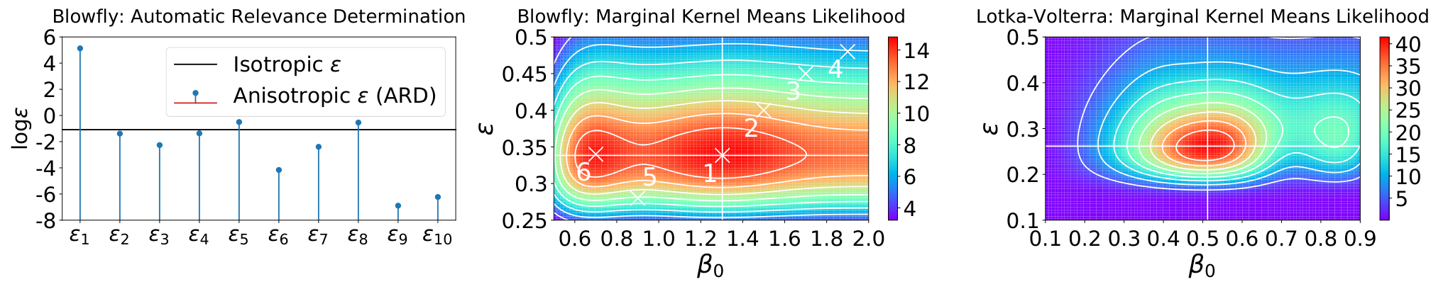
As new simulations become available, we relearn and update the hyperparameters for KELFI by maximizing the MKML. Figure 2 (center) shows an instance of the MKML surface used to learn the hyperparameters for KELFI when using $m=280$ simulations. For KBR and K-ABC we update hyperparameters by the median length heuristic. For K-ABC we also report the case where the heurstic is scaled by a constant denoted with (S), which achieved significantly better accuracy and confirms that the heuristic is often sub-optimal.

Overall, the top three performers are KELFI, KBR, and GPS-ABC. Across a range of simulation calls, KELFI achieves the lowest error. It is also the only method that achieved less than $1\%$ average NMSE within $1000$ simulations and achieves this as early as $300$ simulations. The most competitive methods to KELFI are KBR and GPS-ABC. For these three methods, we also show their variability from best to worst case NMSEs out of the $10$ repeats to visualize their sensitivity to the stochasticity in randomized simulations. This reveals that KELFI is a stable outperformer with comparatively less variability across randomized runs.

We proceed to demonstrate and emphasize the effectiveness and suitability of MKML as a hyperparameter learning objective, using the case with $280$ simulations as an example. Figure 2 (center) illustrates that hyperparameters with a higher MKML (3.3) result in lower NMSE consistently. Notably, even with suboptimal hyperparameter choices, KELFI still achieves competitive average NMSE scores of less than 2.2%. At $280$ simulations, the next best average NMSE score is almost 3% by MCMC-ABC as shown in fig. 3 (left).

Figure 3 (center) suggests that learning the scale $\epsilon$ under MKML reveals an automatic decay schedule which does not have to be set a-priori. As $\epsilon$ controls the scale within which discrepancies between simulations and observations are measured, it is expected that this scale decays as more simulation data is available. Without the MKML, both the initialization of $\epsilon$ and its decay schedule are not straight forward to determine.

In fig. 2 (left), we show that we can perform ARD on the ABC $\epsilon$-kernel $\kappa_{\bm{\epsilon}}$, and hence the kernel $k_{\bm{\epsilon}}$, by using a different $\epsilon_{i}$ for each of the $10$ statistics. We do this by initializing each $\epsilon_{i}$ to the isotropic solution in fig. 2 (center) and further optimize the MKML to learn all $\epsilon_{i}$ jointly. In particular, the first summary statistic describes the average log population numbers nears its troughs (first quartile), and is determined to be comparatively irrelevant (high $\epsilon_{i}$). Meanwhile, the last two statistics describe the number of peaks at two thresholds, and are determined to be comparatively relevant (low $\epsilon_{i}$). This agrees with the intuition that Blowfly population dynamics are highly characterized by its peaks, instead of i its troughs (Wood, 2010).

The Lotka-Volterra simulator describes the time evolution of the populations within a predator-prey system. Only for a small set of parameters does the model simulate a realistic scenario with oscillatory behavior, making the inference task formidably challenging. We follow the exact setup as described in Papamakarios and Murray, 2016. There are 4 parameters and 9 normalized summary statistics. We place the same uniform prior on the log parameters and use the same ground truth parameters. After performing inference on all four parameters, we show in fig. 3 (right) the marginal posterior distribution for $\log{\theta_{1}}$.

KELFI achieves competitive performance using only $2500$ simulations, with both posterior mean and mode close to the true value. The MKML for hyperparameter learning is shown in fig. 2 (right). Posterior mode is obtained by maximizing the KMP. Meanwhile, the three ABC methods used up to $100000$ simulations. While confident, LFVI (Tran et al., 2017a) tends to have a biased posterior mean. For direct comparison, both KELFI and mixture density network (MDN) (Papamakarios and Murray, 2016) use the original prior as the proposal prior. KELFI achieves slightly higher accuracy than MDN which used $10000$ simulations, $4$ times that used for KELFI. Finally, we also similarly use $2500$ simulations for KBR. With the same number of simulations, KELFI achieves higher accuracy in both mean and mode with higher confidence.

References

- Andrieu et al., (2009) Andrieu, C., Roberts, G. O., et al. (2009). The pseudo-marginal approach for efficient monte carlo computations. The Annals of Statistics, 37(2):697–725.
- Beaumont, (2010) Beaumont, M. A. (2010). Approximate bayesian computation in evolution and ecology. Annual review of ecology, evolution, and systematics, 41:379–406.
- Carmeli et al., (2010) Carmeli, C., De Vito, E., Toigo, A., and Umanitá, V. (2010). Vector valued reproducing kernel hilbert spaces and universality. Analysis and Applications, 8(01):19–61.
- Chen et al., (2010) Chen, Y., Welling, M., and Smola, A. (2010). Super-samples from kernel herding. In The Twenty-Sixth Conference Annual Conference on Uncertainty in Artificial Intelligence (UAI-10), pages 109–116. AUAI Press.
- Flaxman et al., (2016) Flaxman, S., Sejdinovic, D., Cunningham, J. P., and Filippi, S. (2016). Bayesian learning of kernel embeddings. In Proceedings of the Thirty-Second Conference on Uncertainty in Artificial Intelligence, pages 182–191. AUAI Press.
- Fukumizu et al., (2004) Fukumizu, K., Bach, F. R., and Jordan, M. I. (2004). Dimensionality reduction for supervised learning with reproducing kernel Hilbert spaces. Journal of Machine Learning Research, 5(Jan):73–99.
- Fukumizu et al., (2013) Fukumizu, K., Song, L., and Gretton, A. (2013). Kernel Bayes’ rule: Bayesian inference with positive definite kernels. Journal of Machine Learning Research, 14(1):3753–3783.
- Grünewälder et al., (2012) Grünewälder, S., Lever, G., Baldassarre, L., Patterson, S., Gretton, A., and Pontil, M. (2012). Conditional mean embeddings as regressors. In Proceedings of the 29th International Conference on Machine Learning, ICML 2012, volume 2, pages 1823–1830.
- Kajihara et al., (2018) Kajihara, T., Kanagawa, M., Yamazaki, K., and Fukumizu, K. (2018). Kernel recursive abc: Point estimation with intractable likelihood. In International Conference on Machine Learning, pages 2405–2414.
- Kanagawa et al., (2016) Kanagawa, M., Nishiyama, Y., Gretton, A., and Fukumizu, K. (2016). Filtering with state-observation examples via kernel monte carlo filter. Neural computation, 28(2):382–444.
- Marin et al., (2012) Marin, J.-M., Pudlo, P., Robert, C. P., and Ryder, R. J. (2012). Approximate Bayesian computational methods. Statistics and Computing, 22(6):1167–1180.
- Marjoram et al., (2003) Marjoram, P., Molitor, J., Plagnol, V., and Tavaré, S. (2003). Markov chain monte carlo without likelihoods. Proceedings of the National Academy of Sciences, 100(26):15324–15328.
- Meeds and Welling, (2014) Meeds, E. and Welling, M. (2014). Gps-abc: Gaussian process surrogate approximate bayesian computation. In Proceedings of the Thirtieth Conference on Uncertainty in Artificial Intelligence, pages 593–602. AUAI Press.
- Mitrovic et al., (2016) Mitrovic, J., Sejdinovic, D., and Teh, Y. W. (2016). DR-ABC: Approximate Bayesian Computation with kernel-based distribution regression.
- Moreno et al., (2016) Moreno, A., Adel, T., Meeds, E., Rehg, J. M., and Welling, M. (2016). Automatic variational abc. stat, 1050:28.
- Muandet et al., (2017) Muandet, K., Fukumizu, K., Sriperumbudur, B., Schölkopf, B., et al. (2017). Kernel mean embedding of distributions: A review and beyond. Foundations and Trends® in Machine Learning, 10(1-2):1–141.
- Nakagome et al., (2013) Nakagome, S., Fukumizu, K., and Mano, S. (2013). Kernel approximate Bayesian computation in population genetic inferences. Statistical applications in genetics and molecular biology, 12(6):667–678.
- Ong et al., (2018) Ong, V. M., Nott, D. J., Tran, M.-N., Sisson, S. A., and Drovandi, C. C. (2018). Variational Bayes with synthetic likelihood. Statistics and Computing, 28(4):971–988.
- Papamakarios and Murray, (2016) Papamakarios, G. and Murray, I. (2016). Fast -free inference of simulation models with bayesian conditional density estimation. In Advances in Neural Information Processing Systems, pages 1028–1036.
- Park et al., (2016) Park, M., Jitkrittum, W., and Sejdinovic, D. (2016). K2-ABC: Approximate Bayesian computation with kernel embeddings.
- Price et al., (2017) Price, L. F., Drovandi, C. C., Lee, A., and Nott, D. J. (2017). Bayesian synthetic likelihood. Journal of Computational and Graphical Statistics, pages 1–11.
- Pritchard et al., (1999) Pritchard, J. K., Seielstad, M. T., Perez-Lezaun, A., and Feldman, M. W. (1999). Population growth of human y chromosomes: a study of y chromosome microsatellites. Molecular biology and evolution, 16(12):1791–1798.
- Rasmussen and Williams, (2006) Rasmussen, C. E. and Williams, C. K. I. (2006). Gaussian processes for machine learning. The MIT Press.
- Sisson et al., (2007) Sisson, S. A., Fan, Y., and Tanaka, M. M. (2007). Sequential monte carlo without likelihoods. Proceedings of the National Academy of Sciences, 104(6):1760–1765.
- Snoek et al., (2012) Snoek, J., Larochelle, H., and Adams, R. P. (2012). Practical bayesian optimization of machine learning algorithms. In Advances in neural information processing systems, pages 2951–2959.
- Song et al., (2013) Song, L., Fukumizu, K., and Gretton, A. (2013). Kernel embeddings of conditional distributions: A unified kernel framework for nonparametric inference in graphical models. IEEE Signal Processing Magazine, 30(4):98–111.
- Song et al., (2009) Song, L., Huang, J., Smola, A., and Fukumizu, K. (2009). Hilbert space embeddings of conditional distributions with applications to dynamical systems. In Proceedings of the 26th Annual International Conference on Machine Learning, pages 961–968. ACM.
- Sriperumbudur et al., (2010) Sriperumbudur, B. K., Fukumizu, K., and Lanckriet, G. R. (2010). On the relation between universality, characteristic kernels and RKHS embedding of measures. In AISTATS, pages 773–780.
- Sriperumbudur et al., (2011) Sriperumbudur, B. K., Fukumizu, K., and Lanckriet, G. R. (2011). Universality, characteristic kernels and RKHS embedding of measures. Journal of Machine Learning Research, 12(Jul):2389–2410.
- Toni et al., (2009) Toni, T., Welch, D., Strelkowa, N., Ipsen, A., and Stumpf, M. P. (2009). Approximate bayesian computation scheme for parameter inference and model selection in dynamical systems. Journal of the Royal Society Interface, 6(31):187–202.
- (31) Tran, D., Ranganath, R., and Blei, D. (2017a). Hierarchical implicit models and likelihood-free variational inference. In Advances in Neural Information Processing Systems, pages 5523–5533.
- (32) Tran, M.-N., Nott, D. J., and Kohn, R. (2017b). Variational Bayes with intractable likelihood. Journal of Computational and Graphical Statistics, 26(4):873–882.
- Wilkinson, (2014) Wilkinson, R. (2014). Accelerating abc methods using gaussian processes. In Artificial Intelligence and Statistics, pages 1015–1023.
- Wood, (2010) Wood, S. N. (2010). Statistical inference for noisy nonlinear ecological dynamic systems. Nature, 466(7310):1102.
Appendix A Theoretical Guarantees on Convergence
We provide theoretical guarantees that establish convergence of the kernel embedding likelihood-free inference (KELFI) framework. Section A.1 begins by summarizing the properties of kernels used in KELFI and introducing relevant quantities. Sections A.2 and A.3 provide an overview of conditional mean embeddings (CMEs) and their empirical estimates respectively in the context of KELFI. Section A.4 establishes general convergence theorems for estimators based on the CME. Using these results, we prove convergence guarantees for the kernel means likelihood (KML), marginal kernel means likelihood (MKML), kernel means posterior (KMP), and kernel means posterior embedding (KMPE) in sections A.5, A.6, A.7 and A.8 respectively.
A.1 Kernel Properties
The KELFI framework uses a data kernel where . We do not assume that and are necessarily the same. For example, it is possible to record observation in which the simulator can never generate or fully recover, such as when . Conversely, it is also possible that the simulator can generate a larger variety of simulations than that is possible to observe, such as when . It can also be neither of such cases such as when an only have some overlap. However, since we assume , the kernel is able to measure the similarity between simulated data and observed data .
The KELFI framework employs bounded symmetric positive definite kernels and . Because they are bounded, we can explicitly denote the following upper bounds to their RKHS norm,