10CCS: Information systems Data stream miningCCS: Information systems Web searching and information discoveryCCS: Information systems Web log analysisCCS: Information systems Query log analysisCCS: Information systems Business intelligenceCCS: Mathematics of computing Time series analysisCCS: Applied computing Forecasting

Shubhra Kanti Karmaker Santu Affiliation: University of Illinois Urbana-Champaign (UIUC) email: karmake2@illinois.edu , Liangda Li Affiliation: Yahoo Research email: liangda@oath.com , Yi Chang Note: this author is also affiliated to College of Computer Science and Technology, Jilin University and Key Laboratory of Symbolic Computation and Knowledge Engineering of Ministry of Education, China Affiliation: College of Artificial Intelligence
Jilin University, Changchun, China email: yichang@acm.org and ChengXiang Zhai Affiliation: University of Illinois Urbana-Champaign (UIUC) email: czhai@illinois.edu

2018; © acmcopyright

Abstract.

Previous work has shown that popular trending events are important external factors which pose significant influence on user search behavior and also provided a way to computationally model this influence. However, their problem formulation was based on the strong assumption that each event poses its influence independently. This assumption is unrealistic as there are many correlated events in the real world which influence each other and thus, would pose a joint influence on the user search behavior rather than posing influence independently. In this paper, we study this novel problem of Modeling the Joint Influences posed by multiple correlated events on user search behavior. We propose a Joint Influence Model based on the Multivariate Hawkes Process which captures the inter-dependency among multiple events in terms of their influence upon user search behavior. We evaluate the proposed Joint Influence Model using two months query-log data from https://search.yahoo.com/. Experimental results show that the model can indeed capture the temporal dynamics of the joint influence over time and also achieves superior performance over different baseline methods when applied to solve various interesting prediction problems as well as real-word application scenarios, e.g., query auto-completion.

Keywords:

User Search Behavior, Joint Influence Model, Multivariate Hawkes Process, Query Log Analysis, Influential Event Identification

1. Introduction

Search Engine optimization has been a vastly studied research area in the past decade. One key component of search engine optimization is analyzing the user search behavior in order to better understand their information need. User search behavior has been studied from multiple perspectives, e.g., user’s own browsing history, click log analysis etc. Recently, how various external factors influence the user search behavior has attracted increasing attention (Karmaker Santu et al. 2017). One important type of external factor is the external events that “significantly” attract the general mass. They trigger user’s thirst for information related to the event and thus, pose influence on how the users search to fulfill their information need. How to model the influence of such external events on user search behavior is the high level research question we study in this paper.

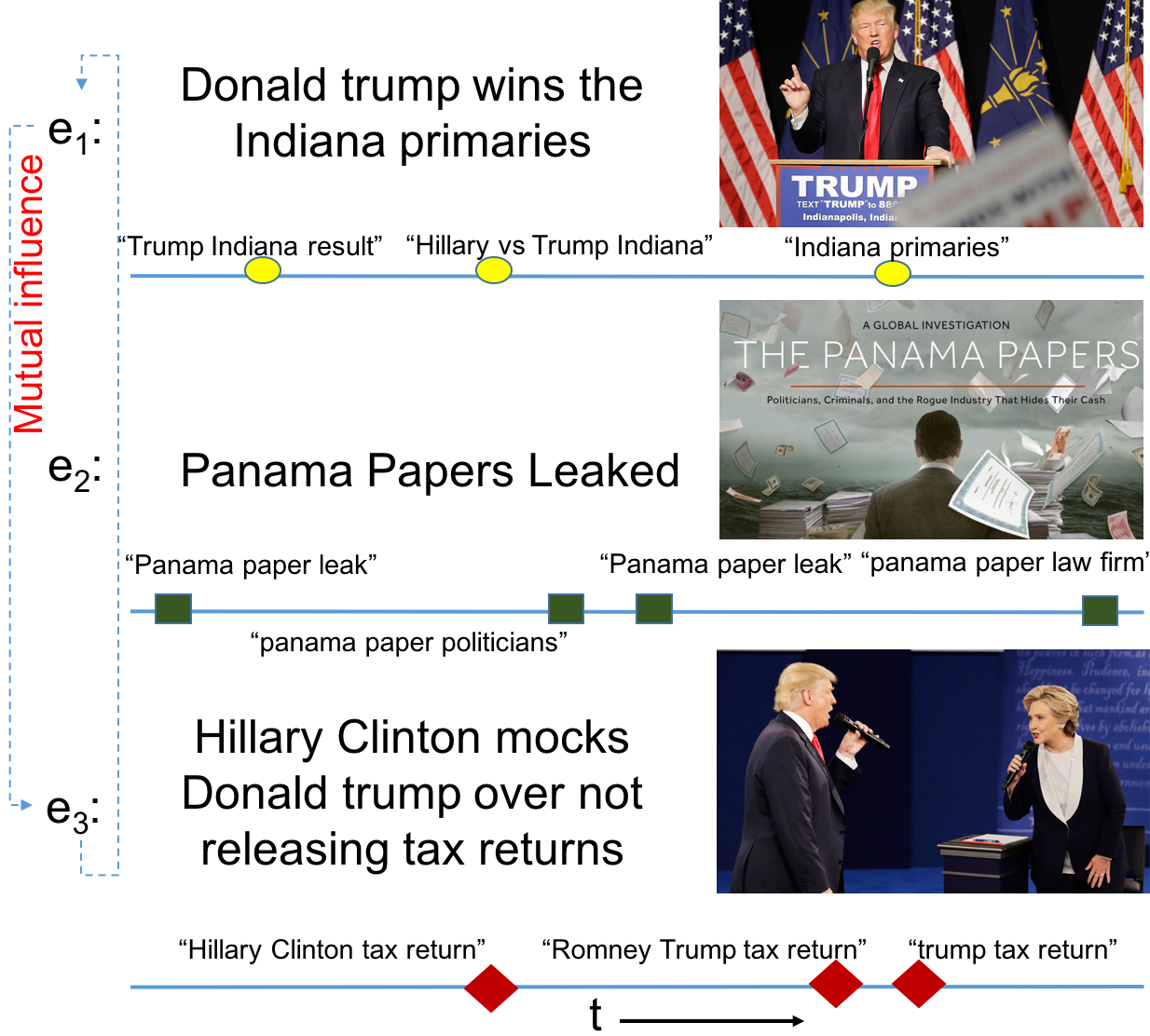
Refer to caption — Figure 1. A toy example with three events $e_{1},e_{2},e_{3}$ . The circles, squares and dices represent queries generated by the influence of event $e_{1}$ , $e_{2}$ and $e_{3}$ respectively.

The problem of modeling the influence of popular trending events on user search behavior is not entirely new, specifically, this problem was introduced by Karmaker et.al. (Karmaker Santu et al. 2017). However, the problem definition provided in (Karmaker Santu et al. 2017) was based on the strong assumption that the influence posed by each event is independent of the other events, which clearly limits the applicability of such solution to cases where there are multiple correlated events and these events pose a joint influence on individual user’s search pattern. To clearly motivate the problem, let us start with the example in Figure 1, where we show three popular events from the month of April, 2016. The first event (denoted by $e_{1}$ ) is Donald Trump’s win in the Indiana Primaries. The blue line below the event description represents the time dimension and the “yellow” dots represent queries related to/triggered by the event $e_{1}$ . For example, the query “Trump Indiana result" is clearly seeking information about Trump’s election results for Indiana Primaries. Note that, the same query can be posed by multiple users at different instants of time. Here, $e_{1}$ is an influential event that has triggered a lot of user queries related to that event. We call these triggered queries as Influenced queries. Similarly, event $e_{2}$ , i.e., “Panama Papers Leaked” and event $e_{3}$ , i.e., “Hillary Clinton mocks Donald Trump over not releasing tax returns” also trigger numerous queries from users asking for relevant information about the respective event. A deeper thought would also reveal that some of these events may be correlated and they may have a joint-influence on the generation of some queries. For example, people searching for “Hillary Clintons mocking about Donald Trump" might also be interested in information about Trump’s Indiana Primary Results and vice-versa. Thus, mutual influence exist among events that jointly affect user search behavior and this joint influence also evolves over time causing corresponding change in the user search pattern. In this paper, we model this evolution of joint influence posed by multiple external events on the search behavior of users.

As mentioned in the previous paragraph, the major limitation of the previous work by Karmaker et.al. (Karmaker Santu et al. 2017) is the assumption that influence posed by one event is independent of the other events. In this paper, we relax this assumption by providing a new problem formulation, i.e., modeling the joint influence posed by multiple events on user search behavior. Specifically, we introduce a new data mining problem, where, given a search query log and a set of (correlated) events, the task is to mine both these datasets to infer the joint influence posed by the provided set of (correlated) events on triggering queries from users. This specifically means, beside measuring the influence of the primary event that triggered the query (lets call it Direct Influence), the task also requires to measure the influence of secondary (correlated) events for the same (lets call it Indirect Influence). This is a new problem because besides computing the degree of influence posed by each event, we also need to come up with a way to compute how their influences are temporally correlated to each other. The joint influence mining task naturally raises many associated interesting research questions, including, how to come up with a numerical formula for measuring influence that is comparable across multiple events (note that, the influence scores computed by Karmaker et.al. (Karmaker Santu et al. 2017) are not directly comparable across multiple events), how influence of multiple events jointly evolve over time and how they correlate in the temporal dimension etc. (see section 3 and section 5.2 for a detailed list of questions).

To solve the joint influence modeling task, we propose a novel mining algorithm based on Multivariate Hawkes Process (Liniger 2009), which is a mutually exciting point process suitable for modeling the frequencies of random events. The joint influence modeling approach proposed by us has several benefits over the independent influence model proposed in (Karmaker Santu et al. 2017); first, it relaxes the assumption that each event poses an influence that is independent of the other events and thus can model real word scenarios better; second, it can capture the temporal correlation of influences posed by two correlated events providing a way to categorize direct influence versus indirect influence and thus can leverage this correlation to better model the evolution of joint influence over time; third, it provides a formal way to measure the influence of multiple events in a comparable numerical scale. Another beneficial feature of the proposed method, as demonstrated by the experimental results (section 6), is that the proposed joint influence model is fairly general and is widely applicable on various interesting prediction tasks and search intent related applications (e.g., query suggestion, query auto-completion) and obtains superior results in comparison to multiple baseline methods. The core contributions of this paper are listed below:

(1)

We introduce the novel problem of modeling the (temporal) dependency across multiple events in terms of the influences posed by them on user search behavior. To the best of our knowledge, this problem has not been studied before.
(2)

We propose a Joint Influence Model based on Multivariate Hawkes Process which captures the joint-influence posed by multiple events on user search behavior as well as models how this joint influence evolves over time.
(3)

We present efficient numerical techniques to compute the likelihood of any query log data w.r.t. the proposed Joint Influence Model; which provides us with a way to estimate the optimal parameters of the model by maximizing the likelihood.
(4)

We evaluate the proposed Joint Influence Model using two months query-log data from https://search.yahoo.com/. Experimental results show that the model can indeed capture the temporal dynamics of the joint influences over time and can be applied to solve various interesting prediction problems as well as real-word application scenarios, e.g., query auto-completion.

2. Related Work

Search query logs have been extensively studied to understand user search behavior and provide better search experience (Jiang et al. 2014; Li et al. 2014; White et al. 2013). Existing work mostly focused on the inference of users’ search intent based on their own search habit and search history. On the other hand, our paper tries to model how user behavior on a search engine is influenced by external factors such as trending events.

Temporal Information Retrieval (Campos et al. 2015; Dakka et al. 2012; Berberich et al. 2010; Kulkarni et al. 2011) and Event Detection (Atefeh and Khreich 2015; Zhou et al. 2015; Walther and Kaisser 2013; Dong et al. 2015; Abdelhaq et al. 2013) are two areas closely related to our work. While Event Detection has been studied vastly in the literature (see (Atefeh and Khreich 2015) for a recent survey), research interest on Temporal Information Retrieval has grown recently (Campos et al. 2015). However, we emphasize that, neither of these is the intended goal of this study and our primary motivation is somewhat orthogonal, i.e., given that some (possibly multiple) events have already been reported, we go one step further to investigate how these events may jointly impact/influence the search behavior of the users.

The notion of event-based retrieval was introduced by Strötgen and Gertz (Strötgen and Gertz 2012) by returning events instead of documents. Zhang et al. (Zhang et al. 2010) addressed the detection of recurrent event queries. Ghoreishi and Sun (Ghoreishi and Sun 2013) introduced a binary classifier for detecting queries related to popular events. Kanhabua (Kanhabua et al. 2015) extended the work (Ghoreishi and Sun 2013) by enabling the classifier to detect less popular queries beside popular ones. However, all these approaches are supervised classification methods and largely depend on the quality of training labels provided by humans, whereas our approach is unsupervised.

Kairam et. al. (Kairam et al. 2013) investigated the online information dynamics surrounding trending events, by performing joint analysis of large-scale search and social media activity. Matsubara et. al. (Matsubara et al. 2015) presented a new model for mining large scale co-evolving online activities. Pekhimenko et al. (Pekhimenko et al. 2015) designed a system named “PocketTrend" that automatically detects trending topics in real time, identified the search content associated to the topics, and then intelligently pushed this content to users’ local machine in a timely manner. However, none of these studies provide answer to the question: how to model the evolution of joint influence posed by multiple events on user search behavior, which is one of the primary motivations of our work. The closest match to this paper is the work by Karmaker et.al. (Karmaker Santu et al. 2017) where they first introduce the problem of modeling the influence of popular trending events on user search behavior. However, as mentioned in section 1, their problem definition was based on the unrealistic assumption that only one event can influence the triggering of a particular query and the influences posed by multiple events are independent of each other. In this paper, our primary focus is to relax these assumptions and propose a more realistic model to capture the joint influence of multiple events.

Another important topic related to this paper is point process, which has been used to model social networks (Blundell et al. 2012) and natural events (Zhuang et al. 2002). People find self-exciting point processes naturally suitable to model continuous-time events where the occurrence of one event can affect the likelihood of subsequent events in the future. One important self-exciting process is Hawkes process, which was first used to analyze earthquakes (Zhuang et al. 2002), and then widely applied to many different areas, such as market modeling (Errais et al. 2010), crime modeling (Stomakhin et al. 2011), conflict (Z.-Mangion et al. 2012), viral videos on the Web (Crane and Sornette 2008) etc. In this work, we propose a novel Joint Influence Model based on multivariate Hawkes process (Liniger 2009) that can capture the dynamics of simultaneous influence by multiple events on user search behavior.

3. Problem Formulation

Let, $E=\{e_{1},e_{2},...,e_{k}\}$ be the set of all events for which we want to analyze their influence on the user search behavior, where $k$ is the total number of events under consideration and each event $e_{j}$ is represented in terms of natural text (for details on the representation of an event, refer to the work by Karmaker et.al. (Karmaker Santu et al. 2017)). Also assume that, each $e_{j}$ is associated with a set of queries that were generated from influence (“to some extent”) by the same event. Let this set be denoted by $Q_{j}=\{q_{j1},q_{j2},....\}$ . Each $q_{ji}$ consists of a tuple < $w_{ji},t_{ji},x_{ji}$ >, where, $w_{ji}$ is the query-text, $t_{ji}$ is the timestamp of receiving the query and $x_{ji}$ is a textual-similarity score between event-text $e_{j}$ and query-text $w_{ji}$ . The higher the similarity between $e_{j}$ and $w_{ji}$ , the higher the $x_{ji}$ score is. For details on how we can get the query set $Q_{j}$ associated with each event $e_{j}$ and how to compute $x_{ji}$ for an event-query pair, please see (Karmaker Santu et al. 2017). We omit the details here due to lack of space.

Given the input data mentioned above, our goal is to model the temporal dynamics of the joint influence posed by different events in $E$ on user search behavior. Specifically, we seek answers to the following questions which were never investigated before: 1) Is there a way to computationally model the dependency among different events in terms of the influences posed by them on user search behavior? 2) How these (correlated) influences of multiple events jointly evolve over time? 3) Given that we have seen a query which is triggered by some event $e_{j}$ , how does that change the future influence of some event other than $e_{j}$ ? 4) Can we use the correlation among multiple events to distinguish between Direct Influence and Indirect Influence (defined in Section 1)? We also ask the same questions raised by Karmaker et.al. (Karmaker Santu et al. 2017), e.g., 5) How the textual similarity between an influential event and an influenced query affects the influence trend of that event? 6) How long the influence of different events last? To provide answers to these questions, we formally introduce a novel Joint Influence Model based on Multivariate Hawkes Process, in the following section.

4. Joint Influence Model

We model the joint influence of multiple events on user search behavior through a generative multivariate point process where each point corresponds to the submission of a new query influenced by some event $e_{j}\in E$ . To be more specific, we propose a new generative model based on Multivariate Hawkes Process (a specific mutually exciting point process) to describe the generation of the influenced queries. This way of modeling query generation is beneficial because this would also allow us to quantify the influence of different events on this generation process at any instant of time. Multivariate Hawkes process is naturally suitable to our problem scenario because it can model the frequencies of occurrences of multiple events in the continuous time domain. For a detailed background on Multivariate Hawkes Process and for further justification on why it is helpful, please refer to (Liniger 2009).

Let, $Q=Q_{1}\cup Q_{2}\cup....\cup Q_{k}$ , be the set of all query submissions which were influenced by some event $e_{j}\in E$ . Additionally, let $Q_{j}$ be the set of all queries that were triggered by the direct influence of event $e_{j}$ . One naive way to collect $Q_{j}$ corresponding to event $e_{j}$ is to retrieve queries from the search log that are textually similar to event-text. For further details on how to retrieve a good quality $Q_{j}$ for event $e_{j}$ , please refer to (Karmaker Santu et al. 2017). For modeling the joint influence, we consider the union set, i.e., $Q$ , where each query $q_{i}\in Q$ corresponds to one point in the multivariate point process and is represented by the tuple < $t_{i}$ , $d_{i}$ , $x_{i}$ >. Here, $t_{i}$ is the timestamp of receiving the the query and thus, always $t_{i}>0$ ; $d_{i}$ is the event which influenced the generation of $q_{i}$ and thus, $d_{i}$ can be any event $e_{j}$ , i.e., $d_{i}\in E$ ; $x_{i}$ is the textual-similarity score between event-text, $text(d_{i})$ and query-text, $text(q_{i})$ .

Given this setup, the core technical challenge in designing the Joint Influence Model boils down to the problem of how we can formally define the multi-event influenced query generation process; in other words, how to fully characterize the multivariate point process? This is not trivial due to the abstractness in the concept of influence. We address this challenge by introducing the notion of Influence Function, which we will discuss in detail in the following section¹¹ 1 All the codes and evaluation scripts for experimentation can be found at the following link: (https://bitbucket.org/karmake2/influencemodeling/src/master/):

4.1. The Influence Function

We characterize the multivariate point process by defining a set of continuous functions $\lambda_{j}$ for $j=\{1,2,....,k\}$ , we call them Influence Functions, which represent the influence of each event $e_{j}\in E$ on the generation of the queries in $Q$ at any instant of time. Designing a suitable $\lambda$ function is the main challenge towards building a reasonable Joint Influence Model. However, defining influence is more of a philosophical question rather than a mathematical one. With this constraint in mind, we adopt to define influence through different components that the final influence function should accommodate and eventually, combine all these components into a single influence function. We first start with various components of the influence function $\lambda_{j}$ .

Base Influence: We assume that there is always a non-negative influence posed by each event $e_{j}\in E$ on the generation of the queries in $Q_{j}$ . Thus, each event $e_{j}$ is associated with a constant $\eta_{j}$ which governs the rate at which we expect to observe new queries influenced by event $e_{j}$ . This gives our first set of parameters for the influence function, i.e., $\eta_{j}\geq 0$ for $j=\{1,2,....,k\}$ . In contrast, the independent influence model proposed by Karmaker et.al. (Karmaker Santu et al. 2017) (let’s call it IIM), has only one parameter $\eta$ for all events.

Decay Functions: The decay functions characterize how the influence of each event diminishes over time. Thus, each event $e_{j}$ is associated with a decay function $w_{j}$ which decides how fast the influence of the same event decays with time. Without loss of generality, we use Exponential Decay functions for our Joint Influence Model. While other forms of the decay function are certainly possible, the investigation of the choosing the right decay function is orthogonal to the goal of this research. Mathematically, Exponential Decay Functions are represented as the following:

w_{j}(t)=\alpha_{j}\exp(-\alpha_{j}t)

The corresponding cumulative decay function is the following (we will need this later):

\bar{w}_{j}(t)=1-\exp(-\alpha_{j}t)

In contrast, IIM (Karmaker Santu et al. 2017) has one decay parameter $w$ for all events.

Impact Functions: Whenever the search engine receives a query triggered by some event $e_{j}$ , we assume that this newly received query increases the influence of all events (not only $e_{j}$ ), which in turn, increases the probability of receiving further queries influenced by different events. The more we receive new (influenced) queries, the higher the influence of different events become; yielding a higher probability of receiving more influenced queries in the future. Thus, the influence of different events as well as frequency of influenced queries we receive mutually grow together, which is similar to the idea of mutually exciting multivariate point processes (Hawkes 1971). Note that, for some event (mostly uncorrelated events), the increment of its influence can be zero which is also expected.

Given that we have received a new query $q_{i}$ (< $t_{i}$ , $d_{i}$ , $x_{i}$ >) triggered by event $d_{i}$ , the amount by which the influences of different events increase depends on the textual-similarity score, i.e. $x_{i}$ , between the event-text and the query-text. This is intuitive because, highly relevant queries are expected to have more impact on the change of influence than less relevant queries. To capture this, we introduce a set of Impact Functions which govern how the influence of all events change depending on the textual-similarity score between the newly received query and its triggering event. Let us denote these Impact Functions by the notation $g_{d_{i}}(x_{i})$ . The interpretation of $g_{d_{i}}(x_{i})$ is as follows: assuming that the newly received query $q_{i}$ was triggered by event $d_{i}$ and the textual similarity between $text(d_{i})$ and $text(q_{i})$ is $x_{i}$ , the influences of all the events are then increased in proportion to $g_{d_{i}}(x_{i})$ .

Note that, reception of query $q_{i}$ increases the influences of all events by the same amount, i.e., by $g_{d_{i}}(x_{i})$ : which is not desirable. To address this issue, we have a whole new set of parameters, namely “Mutual-Influence Co-efficients" which we will discuss shortly after this. However, the purpose of “Impact Functions” is solely to define how the influence of an event changes based on the textual-similarity score between the newly received query $q_{i}$ and its triggering event $d_{i}$ .

Impact functions take the textual similarity score $x_{i}$ as an input parameter. The exact form of Impact Function we choose would thus depend on the distribution of $x_{i}$ , let us call it Intent-Match Distribution. Below we discuss the Intent-Match Distribution briefly, choose a reasonable function for it and then choose the corresponding suitable Impact Function
.

Intent-Match Distribution: Intent-Match Distribution is essentially the distribution of the textual-similarity score between the triggering event and the influenced query. For textual-similarity score, we choose the following modified version of the $BM25$ introduced in the work (Karmaker Santu et al. 2017) (The details of this function and rationale behind choosing it can be found in the paper (Karmaker Santu et al. 2017) ). Let, $W_{E}=<W_{E_{1}},W_{E_{2}},...,W_{E_{n}}>$ be the “event-text” and $W_{q}=<W_{q_{1}},W_{q_{2}},...,W_{q_{n}}>$ be the “query-text”. Then,

x_{i}(W_{E},W_{q})=\sum_{i=1}^{|W_{E}|}\frac{\omega(W_{E_{i}}).IDF(W_{E_{i}}).TF(W_{E_{i}},W_{q}).(k_{1}+1)}{TF(W_{E_{i}},W_{q})+k_{1}.(1-b+b.\frac{|W_{q}|}{avgql})}

(1)

\text{subject to}\sum_{i=1}^{|W_{E}|}\omega(W_{E_{i}})=1

Note that, the textual-similarity score $x_{i}$ is independent of the past history of received queries and solely depends on the similarity between the “event-text" and the “query-text". Further, $x_{i}\geq 0$ .

To specify the Intent-Match Distribution, we hypothesize that a power law probability distribution is the most suitable for our case because of the following reasoning: among the set of all queries that are influenced by some event $e_{j}$ , very few queries would exactly match with the details in the event-text, while a lot of queries intent would match the details only partially or marginally (these are general exploratory queries). The higher the intent-match, the rarer the frequency becomes; in fact, the frequency decreases exponentially with the increase in textual-similarity. Our empirical evaluation also supports this hypothesis (details in section 6.1).

Based on the argument presented above and without loss of generality, we select “Pareto distribution" as our Intent-Match Distribution, which is a popular power law probability distribution. “Pareto distribution" is defined on the half line $[0,\infty)$ and has two parameters $\mu>0$ and $\rho>0$ . Each event $e_{j}$ is associated with a Intent-Match Distribution $f_{j}$ (“Pareto distribution” in this case).

(2)

f_{j}(x)=\frac{\rho_{j}\mu_{j}^{\rho_{j}}}{(x+\mu_{j})^{\rho_{j}+1}}

Under the restriction that $\rho_{j}>2$ , a suitable impact function is the following with parameters $\rho_{j}\geq 0$ , $\mu_{j}\geq 0$ , $\phi_{j}\geq 0$ , $\psi_{j}\geq 0$ (Please see (Liniger 2009) for details and rationale) :

(3)

g_{j}(x)=\frac{(\rho_{j}-1)(\rho_{j}-2)}{\phi_{j}(\rho_{j}-1)(\rho_{j}-2)+\psi_{j}\mu_{j}(\rho_{j}-2)}(\phi_{j}+\psi_{j}x)

Thus, each event $e_{j}$ is associated with a Intent-Match Distribution $f_{j}$ as well as an impact function $g_{j}$ . In contrast, the IIM (Karmaker Santu et al. 2017) has only one impact function $g(x)$ for all events, which was defined as $g(x)=x$ ; whereas, $g_{d_{i}}(x_{i})$ is a generalization of that with more flexibility to capture the impact.

Mutual-Influence Co-efficients: While the impact function captures the relationship between the textual-similarity of an “influenced query-triggering event pair” and the corresponding change in the influence of an event, it fails to distinguish the different impacts the same query might pose for different events. For example, the submission of query “Trump Indiana Results” should directly indicate an increasing influence of the event “Donald Trump wins Indiana primaries” (This is the Direct Influence); however, the same query might have little/no indication about the increasing influence of the event “Messi scores a hat-trick against real madrid” (lets call it No Influence). At the same time, query “Trump Indiana Results” might have an indirect indication about the increasing influence of the correlated event “Hillary Clinton results for Iowa Primaries” (The is the Indirect Influence). Modeling these inter-dependencies among multiple events in terms of the influence posed by them is one of the central key questions we investigate in this paper. Our proposed Joint Influence Model addresses this question by introducing a new set of Co-efficients, we call them Mutual-Influence Co-efficients, which is a unique component of our proposed model.

To capture the three types of influences, i.e., Direct Influence, Indirect Influence, No Influence as mentioned above; we introduce a $k\times k$ matrix of coefficients which we call the Mutual-Influence Co-efficients.

MIC=\begin{bmatrix}\nu_{11}&\nu_{12}&\nu_{13}&\dots&\nu_{1k}\\ \nu_{21}&\nu_{22}&\nu_{23}&\dots&\nu_{2k}\\ \ldots&\ldots&\ldots&\ldots&\ldots\\ \nu_{k1}&\nu_{k2}&\nu_{k3}&\dots&\nu_{kk}\end{bmatrix}

The diagonal elements of the matrix represent Direct Influence, while non-diagonal elements represent Indirect Influence. We also impose the constraint, $\nu_{ji}\geq 0$ for $i,j=\{1,....,k\}$ . A zero value for any element in the $MIC$ matrix represents No Influence, while higher non-zero values indicate Significant Influence. Thus, the $MIC$ matrix contains valuable information about the inter-dependencies among multiple external events in terms of their influence on user search behavior.

Influence Function and Query Generation Process: So far, we have discussed all the components we needed to define our influence function. Below we present the actual definition of the influence function by combining all these components:

(4)

\lambda_{j}(t)=\eta_{j}+\sum_{j=1}^{k}\nu_{ji}\int_{(-\infty,t)\times R}w_{j}(t-s)g_{j}(x)e_{j}(ds\times dx)

Now, we define the mutually-exciting query generation process:

Definition 4.1 (Mutually-Exciting Query Generation Process).

Let us assume that, we observe queries in the form of triples < $t_{i}$ , $d_{i}$ , $x_{i}$ > for $1\leq i\leq n$ , where $t_{i}\in[T_{*},T^{*}]$ and $t_{i}>t_{i-1}$ , $d_{i}\in\{1,2,....,k\}$ and $x_{i}\in R^{+}$ . For the $i$ -th query, it occurs at timestamp $t_{i}$ , the triggering event is $d_{i}$ and the corresponding textual-similarity is $x_{i}$ . At any instant of time $t$ , each event $e_{j}$ for $j=\{1,2,.....,k\}$ has an influence $\lambda_{j}$ defined by equation 4. This constitutes our Generative Multivariate Hawkes Process.

For a Multivariate Hawkes Process to be well defined, we need the following two conditions to be satisfied:

(1)

The maximum of the Eigen Values of the $MIC$ matrix is defined as the spectral radius of $MIC$ , i.e,
$Spr(MIC)=max(eigenValues(MIC))$ . Multivariate Hawkes Process requires the following condition to satisfy:

$Spr(MIC)<1$
(2)

The decay functions must satisfy the following constraints:

$\int_{0}^{\infty}tw_{j}(t)dt<\infty$

Finally, for computational feasibility, we present the numerical version of the continuous influence function in equation 4 below. Let us assume that we have observed queries at points $\{t_{i}\}$ , for $1\leq i\leq n$ . Then, for any timestamp $t_{i}$ , the influence of event $j$ , $\lambda_{j}(t_{i})$ is defined as:

(5)

{\hat{\lambda}_{j}(t_{i})}=\eta_{j}+\sum_{m=1}^{i-1}\nu_{j,d_{m}}w(t_{i}-t_{m})g_{d_{m}}(x_{m})

4.2. Estimation of the Optimal Parameters

This section presents the estimation techniques for the optimal parameter values of the influence function. For this purpose, we define the likelihood function for any observed sequence of queries with respect to the proposed mutually exciting multivariate point process. We find the optimal parameters by maximizing the likelihood of the observed query data. Specifically, the log-likelihood function corresponding to the Mutually-Exciting Query Generation Process (see Definition 4.1) looks like the following:

(6)

\log L=\sum_{j=1}^{d}\int_{[T_{*},T^{*}]\times R}\log\lambda_{j}(t)e_{j}(dt\times dx)+\sum_{j=1}^{k}\int_{[T_{*},T^{*}]\times R}\log f_{j}(x)e_{j}(dt\times dx)-\sum_{j=1}^{k}\Lambda_{j}(T^{*})

Here, $T^{*}$ is the upper bound of the observation period and $\hat{\Lambda}_{j}(T^{*})$ is called the compensator function and is defined as follows:

(7)

\Lambda_{j}(t)=\eta_{j}(t-T_{*})+\sum_{m=1}^{k}\nu_{jm}\int_{(-\infty,t)\times R}[\hat{w}_{j}(t-u)-\hat{w}_{j}(T_{*}-u)]g_{m}(x)e_{m}(du\times dx)

Numerical Computation: For computational feasibility, we now present the way to numerically compute the log-likelihood function defined in Eqn (6). Specifically, the numerical version of the log-likelihood function takes the following form:

(8)

\log\hat{L}=\sum_{i=1}^{n}\log\hat{\lambda}_{d_{i}}(t_{i})+\sum_{i=1}^{n}\log f_{d_{i}}(x_{i})-\sum_{j=1}^{k}\hat{\Lambda}_{j}(T^{*})

While computation of $f_{d_{i}}(x_{i})$ is straight-forward from equation 2, computation of $\hat{\lambda}_{d_{i}}(t_{i})$ and $\hat{\Lambda}_{j}(T^{*})$ are more involved. Below we present the exact formulas to compute $\hat{\lambda}_{j}(t_{i})$ and $\hat{\Lambda}_{j}(T^{*})$ omitting the derivation details due to lack of space. We assume exponential decay function, i.e., $w_{j}=\alpha_{j}\exp(-\alpha_{j}t)$ , for the exact computational formula, while other forms of decay functions are certainly possible.

(9)

\hat{\lambda}_{j}(t_{i})=\eta_{j}+[\lambda_{j}(t_{i-1})-\eta_{j}]\exp[-\alpha_{j}(t_{i}-t_{i-1})]+\nu_{j,d_{i-1}}g_{d_{i-1}}(x_{i-1})\alpha_{j}\exp[-\alpha_{j}(t_{i}-t_{i-1})]

(10)

\hat{\Lambda}_{j}(T^{*})=\eta_{j}(T^{*}-T_{*})+\sum_{i=1}^{n}\nu_{j,d_{i}}\bar{w}_{j}(t^{*}-t_{i})g_{d_{i}}(x_{i})

By plugging in equation 2, 9 and 10, we obtain the complete numerical version of the log-likelihood function as follows:

(11)

\log\hat{L}=\sum_{i=1}^{n}\log\left\{\eta_{j}+[\lambda_{j}(t_{i-1}-\eta_{j})]\exp[-\alpha_{j}(t_{i}-t_{i-1})]+\nu_{j,d_{i-1}}g_{d_{i-1}}(x_{i-1})\alpha_{j}\exp[-\alpha_{j}(t_{i}-t_{i-1})]\right\}+\sum_{i=1}^{n}\log\left(\frac{\rho_{d_{i}}\mu_{d_{i}}^{\rho_{d_{i}}}}{(x+\mu_{d_{i}})^{\rho_{d_{i}}+1}}\right)-\sum_{j=1}^{k}\left\{\eta_{j}(T^{*}-T_{*})+\sum_{i=1}^{n}\nu_{j,d_{i}}\bar{w}_{j}(t^{*}-t_{i})g_{d_{i}}(x_{i})\right\}

Here, $g_{d_{i}}(x_{i})$ is defined by as:

g_{d_{i}}(x)=\frac{(\rho_{d_{i}}-1)(\rho_{d_{i}}-2)}{\phi_{j}(\rho_{d_{i}}-1)(\rho_{d_{i}}-2)+\psi_{d_{i}}\mu_{d_{i}}(\rho_{d_{i}}-2)}(\phi_{d_{i}}+\psi_{d_{i}}x)

Given the log-likelihood function in equation 11, the set of parameters associated with it is the following:

(12)

\Theta=\left\{\eta_{j},\alpha_{j},\nu_{ji},\rho_{j},\mu_{j},\phi_{j},\psi_{j}\right\}\text{, where $(1\leq i,j\leq k)$}

Incorporating L2 regularization, the optimization problem to find the optimal parameter set $\Theta^{*}$ is written as follows:

(13)

\Theta^{*}=\argmax_{\Theta}\left(\log\hat{L}(\Theta)-||\Theta||\right)

Here, $||\Theta||$ is the L-2 norm of the parameter vector $\Theta$ . One can use any non-linear optimization method to solve this maximization problem. Nelder-Mead Simplex Method (Glaudell et al. 1965) is one such popular optimization technique. Another useful approach is the Sequential Least SQuares Programming (SLSQP) (Boggs and Tolle 1995).

5. Experimental Design

5.1. Data-set

Due to the absence of any readily available joint event-query dataset, we decided to create one from two sets of available data-sets: one for popular events and one for user query history. We call these two data sets Event dataset and Query-Log dataset respectively. The following two paragraphs provide details about these two data-sets.

Event data-set: An obvious choice for a text data set describing events is news articles (though other data such as social media might also be applicable). The NYTimes Developers Network (thanks to them) provides a very useful api called “The Most Popular API" (NYT 2016), which automatically provides the url’s of the most e-mailed, most shared and most viewed articles from NYTimes.com during the last month from the date of the issue of the query. We chose to use this API because of two major benefits: 1) it automatically removes duplicate articles, thus we don’t need to deal with cases where multiple articles are related to the same event. 2) it only provides the most popular articles from NYTimes, thus the quality/accuracy of the events represented by these articles is very high. Using this API, we collected the most e-mailed, most shared and most viewed articles for the month: April, 2016. Each article consists of a tuple <title-text, body-text, timestamp>. Among different categories of news, we used four categories for our experiments: US (National Affairs), Movies, Sports and World (International Affairs).

Query-Log data-set: To analyze the user queries contemporary to the articles in Event data-set, we use the two-months (April and May, 2016) user query log data from the widely used search engine at https://search.yahoo.com/. Each query submission $q$ is represented as a tuple < $query$ - $text$ , $timestamp$ >. The two-months query log data contains $105,925,732$ query submissions in total.

Query-Event Joint data-set: To create the Query-Event Joint data-set, for each article $e_{j}$ in the Event data-set, we retrieved top relevant queries that have at least a similarity score of $1.25$ (with respect to $e_{j}$ ) according the textual similarity function in equation 1 and discarded the rest. This filtering step is reasonable because if the textual similarity is very low (less than $1.25$ ), we assume that there is no influence of $e_{j}$ on the query. This process provides us with a set of influenced queries triggered by each event from the Event data-set. The summary of this data-set is presented in Table 1.

Section	Total	Avg.	Avg.	Total	Avg.
	# of	Title	Body	# of	Textual
	events	Length	Length	queries	Sim.
Movies	25	18.88	458.08	193,282	2.49
Sports	15	19.53	508.4	616,449	2.48
US	18	20.38	487.77	204,926	1.99
World	11	18.18	438.81	22,197	1.96

Table 1. Description of Event-Query Joint Dataset

5.2. Qualitative Evaluation of the Model

It is not possible to do a direct quantitative evaluation of the influence model due to the lack of ground truth information. Thus, to evaluate the quality of the proposed Joint Influence Model, we do a formal investigation of the optimal parameters learnt through the optimization process as described in section 4.2. Below, we present the specific research questions we ask to evaluate the model quality and provide the roadmap of how we can answer each question.

Research Questions:

(1)

Is the “Query Generation Process” well-defined ?
The “Query Generation Process” is well defined only if the Spectral Radius of the Mutual-Influence Coefficient Matrix is less than 1, i.e, $Spr(MIC)<1$ . [see section 4.1 for more details]
(2)

How to compare influences posed by different events?
We can answer this question by computing average influence posed by each event and then compare them. The average influence vector where each element is the average influence of the corresponding event can be obtained using the following formula: $(\mathbbm{1}_{k}-MIC)^{-1}\bm{\eta}$ , where, $\mathbbm{1}_{k}$ is a $k\times k$ identity matrix.
(3)

How to compare Direct Vs Indirect influence ?
The diagonal elements of matrix $MIC$ represent the Direct Influence, whereas, the non-diagonal elements present Indirect Influence. We can do direct numeric comparison here.
(4)

How to measure the influence longevity of an event?
The $\bm{\alpha}$ parameter defines how fast the influence of any event decays over time. Higher values of $\alpha$ denotes a faster decay.
(5)

Is “Pareto Dist." suitable for “Intent Match Dist."?
To answer this question, we look at the empirical distribution of “Intent Match" score between event-text and query text and verify whether “Pareto Distribution" is a good match for it.
(6)

How well the Model fit the original data?
This question can be answered by jointly plotting the simulated influence of an event and the actual frequency of queries generated by that event over the same period of time and see if the trend of the simulated influence is similar to the trend of the actual frequency of generated queries.

5.3. Applications and Quantitative Evaluation

In this section, we demonstrate the wide applicability of the proposed “Joint Influence Model” by demonstrating how the model could be used to solve various interesting prediction problems as well as real-world problems associated with search engine systems. Another benefit of these experiments is to conduct indirect quantitative evaluation of the Joint Influence Model as direct evaluation is impossible due to the lack of ground truth data for influence which is an abstract concept. The primary purpose of these experiments is to see if modeling the influence inter-dependencies among multiple events actually help us achieve better performance in real life application scenarios. To achieve these goals, we present a set of prediction tasks / application scenarios and provide a roadmap on how we can adopt the “Joint Influence Model’ to solve these tasks.

Application Tasks:

(1)

Predict the most influential event in the future:
We assume the influence of an event in the current hour is proportional to the frequency of queries generated by it in the next hour. Thus, the event with the highest influence score in the current hour is predicted to be the event that generates highest number queries in the next hour. We then compare this predicted most influential event with the actual most influential event (computed from the original query log) and based on that, we can report the accuracy of the prediction for a separate held-out testing set.
(2)

Rank multiple events based on their future influences:
This prediction problem is similar to previous prediction problem, except that, now we want to predict the ranking of events in terms of their future influence instead of just predicting the future top influential event. Again, we use the current hour influence scores to predict the next hour’s generated query frequencies and rank the events accordingly. To evaluate the quality of the ranking, we compare the predicted ranking against the actual ranking obtained from the query log and compute two different popular ranking evaluation metrics: i.e, NDCG (Wang et al. 2013) and Rank Biased Overlap (RBO) (Webber et al. 2010).
(3)

Predict the most frequent query in the future:
This prediction problem is the same as the prediction problem in (1) except that now we want to predict the most frequent query in the future instead of the most influential event. For this prediction task, we use a slightly modified version of the original “Joint Influence Model” where apart from computing the evolving influence at the event level, we also compute the evolving influence at the query level. The basic idea is to break each event-level influence into smaller units where each unit would correspond to the query level. We omit the full details of process due to lack of space.
(4)

Rank queries based on their future frequencies:
This prediction problem is similar to the prediction problem in (2) except that now we want to rank queries instead of events. Again we report NDCG (Wang et al. 2013) and Rank Biased Overlap(RBO) (Webber et al. 2010) to evaluate the quality of the predicted ranking.
(5)

Solve a real world application problem, e.g., query auto completion task:
Finally, we select Query Auto Completion as a goal task and use our proposed “Joint Influence Model” to solve it. Specifically, for a new query from the testing set, we look at the first word and try to predict the exact query based on the latest available influence scores of all the queries starting with the first word. Based on these influence scores, we rank the potential queries and then, compute the reciprocal rank of the actual query in the predicted ranked list. We repeat the whole process for all the queries in a separate held-out testing set and report the mean reciprocal rank (MRR) (Voorhees et al. 1999), which is the most popular evaluation metric used in measuring the performance of query auto completion tasks.

Baseline Methods: For all the quantitative evaluation tasks, we compare the proposed Joint Influence Model against the obvious baseline method, i.e., Independent Influence Model (We call it “IIM") introduced in (Karmaker Santu et al. 2017). If the Joint Influence Model( JIM) performs better than IIM, we can conclude that capturing inter-dependencies is indeed useful and can help us achieve superior performance in real life applications. Additionally, as all these quantitative evaluation tasks are some kind of forecasting problems, we also use some popular time series prediction methods as the baselines including Autoregressive Models (AR), Vector Auto Regression (VAR) etc. Note that, our primary focus is not the quantitative evaluation, rather demonstrating the usefulness of capturing influence inter-dependencies among different events. Thus, experimenting with many different forecasting methods is an orthogonal direction with respect to our focus which we do not explore in this work. We also include the simplest baseline method Naive Frequency (NF), where the current hour’s frequency is used to predict the next hour’s frequency. Table 2 lists down all the methods we experimented and also provides with an acronym for each method for notational convenience. JIM is the “Joint Influence Model" proposed in this paper, whereas, “JIM-G" is a minor variation of “JIM" with the constraint that events share the same $\alpha$ , i.e., the decay parameter.

Acronym	Method
NF	Naive Frequency
AR	Auto Regression (Chatfield 2016)
ARD	Auto Regression with difference (Chatfield 2016)
VAR	Vector Auto Regression (Box et al. 2015)
IIM	Independent Influence Model (Karmaker Santu et al. 2017)
JIM	Joint Influence Model
JIM-G	Joint Influence Model-Generalized

Table 2. Methods Compared for Quantitative Evaluation

6. Results

6.1. Qualitative Evaluation of the Model

First, we do a qualitative investigation of the optimal parameters learnt through the optimization process as described in section 4.2. Table 3 presents these learnt parameters. While the individual numbers in Table 3 are not very meaningful, the comparison across different categories of events is quite interesting. For example, $\eta$ for “Sports" category ( $0.3170$ ) is generally much higher than that for “World" category ( $0.0740$ ), suggesting that the general interest in “Sports" events is much higher than “World" events among the common mass. Another interesting parameter is $\alpha$ , which indicates the longevity of influence for different categories of events. According to Table 3, “World" events ( $\alpha=0.6770$ ) usually have a longer lasting influence compared to “Sports" events ( $\alpha=1.1999$ ). Next, we move onto providing answers to the specific research questions asked in section 5.2, sequentially one at a time.

parameter	$\eta$	$\alpha$	$\rho$	$\mu$	$\phi$	$\psi$
Movies	0.1961	0.8697	4.9706	3.0197	0.4542	0.1644
Sports	0.317	1.1999	6.2745	4.2272	1.1608	0.5304
US	0.2328	1.0999	6.3056	1.777	0.6962	0.508
World	0.074	0.677	3.9747	1.5226	0.2465	0.1685

Table 3. Parameters learnt for different categories of events

Is the “Query Generation Process” well defined?
Table 4 shows the spectral radius of Mutual-Influence Co-efficient Matrix obtained for different categories of events. It is evident that, all the numbers are less than 1. Thus, we conclude that, the “Query generation process” is indeed well defined.

Movies (0.9319)

Sports (0.9649)

US (0.9192)

World (0.9213)

Table 4. Spectral Radius of MIC Mat. for different categories

How to compare influences posed by different events?
Table 5 reports the top 2 influential events from each category along with their average influence score computed by the formula presented in section 5.2. For example, the movie “Captain America: Civil War" was found to be the most influential event in the “Movies" Category with an average influence score of $11.5514$ , while “Donald trump Vs Hillary Clinton" was found to be the most influential event (average score 14.0117) in the “US" category. Manual inspection reveals that all these reported influential events are indeed popular events which match with our intuition.

	Sections
Events	Movies	Sports	US	World
$1$	Movie: “Captain America: Civil War” (11.5514)	Horse-Racing: Kentucky Derby (13.5346)	Donald trump Vs Hillary Clinton (14.0117)	Panama Papers Released (0.8179)
$2$	Movie: “X-men: Apocalypse” (2.0532)	Basketball: Stephen Curry (6.6432)	Las Vegas Squatters Housing Collapse (9.6340)	Philippine Presidential Race ( 0.5821)

Table 5. Top two most influential events from four different Categories

How to compare Direct Vs Indirect influence ?
Table 6 reports the average of the diagonal elements (Direct Influence) as well as the non-diagonal elements (Indirect Influence) of the MIC matrix for each category of events. It is evident that the influence posed by the triggering event, i.e., Direct Influence is significantly larger than that of a non-triggering event, i.e., Indirect Influence which also concur with our expectation. For example, Direct Influence ( $0.6342$ ) of events in the “US" category is much higher than the Indirect Influence ( $0.0201$ ) in the same category. In fact, this observation holds for any category.

Influence	Movies	Sports	US	World
Direct	0.5285	0.6495	0.6342	0.5798
Indirect	0.0255	0.0165	0.0201	0.0166

Table 6. Direct Influence Vs Indirect Influence

How to measure the influence longevity of an event?
Direct inspection of $\alpha$ values from Table 3 can provide answer to this question. For example, Table 3 suggests that “Sports" events generally have short term influence ( $\alpha=1.1999$ ), while “World" events have comparatively long lasting influence ( $\alpha=0.6770$ ).

Is “Pareto Dist." suitable for “Intent Match Dist."?
To answer this question, we show the plot for the empirical distribution of “Intent Match" score between event-text and query-text for the events of “Sports" category in Figure 2. This figure demonstrates that as the “Intent Match" score goes high, the number of queries with corresponding score becomes exponentially smaller, suggesting that, indeed “Pareto Distribution" is a reasonable candidate for the “Intent Match Distribution".

How well the Model fits the original data?
We plot the the simulated influence of the event “release of movie Captain America: Civil War" from the “Movies" category along with the actual frequency of queries generated by that event during the same span of time (hour 1500 to hour 1700) in Figure 3. It is clearly evident that the simulated influence can indeed capture the trend of the actual frequency of generated queries and thus, we conclude that the model can indeed capture the influence trend with a decent accuracy.

6.2. Applications and Quantitative Evaluation

This section presents the quantitative evaluation results for the five different application tasks presented in section 5.3, namely, Predict the most influential event in the future [Table 8], Rank multiple events based on their future influences [Table 8], Predict the most frequent query in the future [Table 11], Rank queries based on their future frequencies [Table 11], Solve a real world application problem, e.g., query auto completion task [Table 11]. General inspection of Table[8-11] reveals that, “JIM-G" is found to be the most robust method for all these different application tasks by obtaining the highest number for performance metrics most of the time. For example, for the task “Predict the most influential event in the future" [Table 8], “JIM-G" is found to achieve the highest accuracy for all four categories of events. For the “Query auto completion task", the mean reciprocal rank for “JIM-G" is found to be the highest for all categories except the category “World", for which “IIM" obtains a slightly better number.

In case of event level predictions (Table 8 and 8), $JIM$ turns out to be the second best performing method. This suggests that the Joint Influence Model indeed captures useful information which results in its superior performance over other baseline methods. The superiority of “JIM-G" over “JIM" may be explained by the fact that, while “JIM" has more parameters for $\alpha$ (i.e., one $\alpha$ for each single event) than “JIM-G" (i.e., single $\alpha$ for all events), “JIM" might be suffering from over-fitting the training data while “JIM-G" would learn a more general model suitable across multiple events. This over-fitting problem seems more prominent for query level predictions (Table 11 and 11), especially for category “World" where the number of queries in the dataset is comparatively very small (Table 1). Here, “JIM" cannot even achieve the second best performance. We believe this is due to the sparsity of query level data. Interestingly, the simple baseline “NF", achieves quite good result at the query level prediction problems, while “VAR" suffers severely from overfitting. However, “JIM-G" still performs the best for most of the cases in query level predictions.

In summary, Table[8-11] suggest that the Joint Influence Model is quite robust and useful in many different applications with superior performance over a number of reasonable baseline methods.

Metric	Methods	Movies	Sports	US	World
	NF	0.6638	0.6647	0.9302	0.5073
	AR	0.7256	0.6818	0.8959	0.3934
	ARD	0.7445	0.4249	0.9388	0.0609
Accuracy	VAR	0.7399	0.4997	0.5105	0.1237
	IIM	0.7193	0.6162	0.9376	0.5671²
	JIM	0.7520²	0.6938²	0.9491²	0.5307
	JIM-G	0.7531¹	0.6967¹	0.9542¹	0.5905¹

Table 7. Predicting the most influential event in future

Metric	Methods	Movies	Sports	US	World
	NF	0.9074	0.9105	0.9792	0.7798
	AR	0.9370	0.9168	0.9460	0.6951
	ARD	0.8604	0.7458	0.9529	0.4358
NDCG	VAR	0.8831	0.7914	0.8950	0.5175
	IIM	0.9348	0.8975	0.9831	0.8393²
	JIM	0.9485²	0.9278²	0.9870²	0.8275
	JIM-G	0.9508¹	0.9322¹	0.9879¹	0.8517¹
	NF	0.6596	0.6800	0.8573	0.5140
	AR	0.7052	0.6821	0.7695	0.3967
	ARD	0.5320	0.4122	0.7267	0.0942
RBO	VAR	0.5752	0.4808	0.6331	0.1647
	IIM	0.6961	0.6479	0.8597	0.5992²
	JIM	0.7194²	0.6980²	0.8672²	0.5623
	JIM-G	0.7252¹	0.7069¹	0.8705¹	0.6087¹

Table 8. Predicting future influences of multiple events (Wilcoxon’s signed rank test at level 0.05)

Metric	Methods	Movies	Sports	US	World
	NF	0.3281	0.4894²	0.5717²	0.3879
	AR	0.3879¹	0.4794	0.5400	0.4504
	ARD	0.2424	0.1965	0.4410	0.0443
Accuracy	VAR	0.0023	0.0007	0.0029	0.0001
	IIM	0.3413	0.3660	0.5408	0.4710¹
	JIM	0.3642	0.4688	0.5563	0.3035
	JIM-G	0.3820²	0.5134¹	0.5843¹	0.4544²

Table 9. Predicting the most frequent query in future

Metric	Method	Movies	Sports	US	World
	NF	0.5914	0.6693	0.8060	0.4465
	AR	0.6713²	0.7440²	0.7789	0.5200
	ARD	0.2642	0.2977	0.4717	0.0827
NDCG	VAR	0.0087	0.0052	0.0136	0.0015
	IIM	0.6355	0.6976	0.8121²	0.6555¹
	JIM	0.6484	0.7204	0.8022	0.4809
	JIM-G	0.6870¹	0.7650¹	0.8430¹	0.6062²
	NF	0.4349	0.5707	0.6491	0.3665
	AR	0.4947²	0.5908²	0.6102	0.4130
	ARD	0.1803	0.2191	0.3237	0.0538
RBO	VAR	0.0042	0.0019	0.0045	0.0001
	IIM	0.4562	0.5174	0.6509²	0.4676¹
	JIM	0.4782	0.5724	0.6436	0.3048
	JIM-G	0.5059¹	0.6172¹	0.6764¹	0.4332²

Table 10. Predicting future frequencies for multiple queries. (Wilcoxon’s signed rank test at level 0.05)

Metric	Methods	Movies	Sports	US	World
	NF	0.6427	0.8427	0.8489	0.6899
	AR	0.7382	0.9129	0.8339	0.7471
	ARD	0.2842	0.4077	0.5238	0.2754
MRR	VAR	0.1911	0.1722	0.1186	0.3696
	IIM	0.7839	0.9171	0.8896	0.9262¹
	JIM	0.8082²	0.9509²	0.8903²	0.8999
	JIM-G	0.8226¹	0.9556¹	0.8988¹	0.9193²

Table 11. Query Auto-Completion Results: MRR reported. (Wilcoxon’s signed rank test at level 0.05)

7. Conclusion

The assumption that each popular event poses influence upon user search behavior independently is unrealistic as many real world events are closely related to each other. The primary contribution of this paper is to relax this unrealistic assumption made in the previous work by proposing a Joint Influence Model based on multivariate Hawkes Process that captures the inter-dependency of multiple events in terms of the influence posed by them upon user search behavior. Experimental results demonstrate that the proposed method not only effectively capture the temporal dynamics of joint influences by multiple events, but also when applied to various application tasks, achieves superior performance most of the time over different baseline methods that do not consider this mutual-influence among multiple events. This signifies that the mutual influence which exists among multiple correlated events is an important factor which should be considered while designing such influence models.

8. Acknowledgement

This material is based upon work supported in part by the National Science Foundation under Grant Numbers CNS-1408944 , CNS-1513939, and IIS-1629161.

References

(1)
NYT (2016) 2016. The Most Popular API: NYtimes Developers Network. https://developer.nytimes.com/most_popular_api_v2.json#/README. Accessed: 2016-07-30.
Abdelhaq et al. (2013) Hamed Abdelhaq, Christian Sengstock, and Michael Gertz. 2013. Eventweet: Online localized event detection from twitter. Proceedings of the VLDB Endowment 6, 12 (2013), 1326–1329.
Atefeh and Khreich (2015) Farzindar Atefeh and Wael Khreich. 2015. A survey of techniques for event detection in twitter. Computational Intelligence 31, 1 (2015), 132–164.
Berberich et al. (2010) Klaus Berberich, Srikanta Bedathur, Omar Alonso, and Gerhard Weikum. 2010. A language modeling approach for temporal information needs. In European Conference on Information Retrieval. Springer, 13–25.
Blundell et al. (2012) C. Blundell, K. A Heller, and J. M Beck. 2012. Modelling Reciprocating Relationships with Hawkes Processes. NIPS (2012).
Boggs and Tolle (1995) Paul T Boggs and Jon W Tolle. 1995. Sequential quadratic programming. Acta numerica 4 (1995), 1–51.
Box et al. (2015) George EP Box, Gwilym M Jenkins, Gregory C Reinsel, and Greta M Ljung. 2015. Time series analysis: forecasting and control. John Wiley & Sons.
Campos et al. (2015) Ricardo Campos, Gaël Dias, Alípio M Jorge, and Adam Jatowt. 2015. Survey of temporal information retrieval and related applications. ACM Computing Surveys (CSUR) 47, 2 (2015), 15.
Chatfield (2016) Chris Chatfield. 2016. The analysis of time series: an introduction. CRC press.
Crane and Sornette (2008) R. Crane and D. Sornette. 2008. Robust Dynamic Classes Revealed by Measuring the Response Function of a Social System. Proceedings of the National Academy of Sciences of the United States of America 105, 41 (2008), 15649–15653.
Dakka et al. (2012) Wisam Dakka, Luis Gravano, and Panagiotis Ipeirotis. 2012. Answering general time-sensitive queries. IEEE Transactions on Knowledge and Data Engineering 24, 2 (2012), 220–235.
Dong et al. (2015) Xiaowen Dong, Dimitrios Mavroeidis, Francesco Calabrese, and Pascal Frossard. 2015. Multiscale event detection in social media. Data Mining and Knowledge Discovery 29, 5 (2015), 1374–1405.
Errais et al. (2010) E. Errais, K. Giesecke, and L. R. Goldberg. 2010. Affine Point Processes and Portfolio Credit Risk. SIAM J. Fin. Math. 1, 1 (Sep 2010), 642–665.
Ghoreishi and Sun (2013) Seyyedeh Newsha Ghoreishi and Aixin Sun. 2013. Predicting event-relatedness of popular queries. In Proceedings of the 22nd ACM international conference on Information & Knowledge Management. ACM, 1193–1196.
Glaudell et al. (1965) Rebecca Glaudell, Rogelio Tomas Garcia, and Javier Barranco Garcia. 1965. Nelder-Mead Simplex Method. Computer Journal 7 (1965), 308–313.
Hawkes (1971) Alan G Hawkes. 1971. Spectra of some self-exciting and mutually exciting point processes. Biometrika (1971), 83–90.
Jiang et al. (2014) Jiepu Jiang, Daqing He, and James Allan. 2014. Searching, browsing, and clicking in a search session: changes in user behavior by task and over time. In ACM SIGIR.
Kairam et al. (2013) S. Kairam, M. Morris, J. Teevan, D. Liebling, and S. Dumais. 2013. Towards Supporting Search over Trending Events with Social Media. In International AAAI Conference on Web and Social Media.
Kanhabua et al. (2015) Nattiya Kanhabua, Tu Ngoc Nguyen, and Wolfgang Nejdl. 2015. Learning to detect event-related queries for web search. In Proceedings of the 24th International Conference on World Wide Web. ACM, 1339–1344.
Karmaker Santu et al. (2017) Shubhra Kanti Karmaker Santu, Liangda Li, Dae Hoon Park, Yi Chang, and Chengxiang Zhai. 2017. Modeling the Influence of Popular Trending Events on User Search Behavior. In Proceedings of the 26th International Conference on World Wide Web Companion. International World Wide Web Conferences Steering Committee, 535–544.
Kulkarni et al. (2011) Anagha Kulkarni, Jaime Teevan, Krysta M Svore, and Susan T Dumais. 2011. Understanding temporal query dynamics. In Proceedings of the fourth ACM international conference on Web search and data mining. ACM, 167–176.
Li et al. (2014) Liangda Li, Hongbo Deng, Anlei Dong, Yi Chang, and Hongyuan Zha. 2014. Identifying and labeling search tasks via query-based hawkes processes. In ACM SIGKDD.
Liniger (2009) Thomas Josef Liniger. 2009. Multivariate hawkes processes. Ph.D. Dissertation. SWISS FEDERAL INSTITUTE OF TECHNOLOGY ZURICH.
Matsubara et al. (2015) Yasuko Matsubara, Yasushi Sakurai, and Christos Faloutsos. 2015. The web as a jungle: Non-linear dynamical systems for co-evolving online activities. In WWW, 2015. 721–731.
Pekhimenko et al. (2015) G. Pekhimenko, D. Lymberopoulos, O. Riva, K. Strauss, and D. Burger. 2015. PocketTrend: Timely Identification and Delivery of Trending Search Content to Mobile Users. In WWW, 2015.
Stomakhin et al. (2011) A. Stomakhin, M. B. Short, and A. L. Bertozzi. 2011. Reconstruction of missing data in social networks based on temporal patterns of interactions. Inverse Problems. 27, 11 (Nov 2011).
Strötgen and Gertz (2012) Jannik Strötgen and Michael Gertz. 2012. Event-centric search and exploration in document collections. In Proceedings of the 12th ACM/IEEE-CS joint conference on Digital Libraries. ACM, 223–232.
Voorhees et al. (1999) Ellen M Voorhees et al. 1999. The TREC-8 Question Answering Track Report.. In Trec, Vol. 99. 77–82.
Walther and Kaisser (2013) Maximilian Walther and Michael Kaisser. 2013. Geo-spatial Event Detection in the Twitter Stream.. In ECIR. Springer, 356–367.
Wang et al. (2013) Yining Wang, Liwei Wang, Yuanzhi Li, Di He, Wei Chen, and Tie-Yan Liu. 2013. A theoretical analysis of NDCG ranking measures. In Proceedings of the 26th Annual Conference on Learning Theory (COLT 2013).
Webber et al. (2010) William Webber, Alistair Moffat, and Justin Zobel. 2010. A similarity measure for indefinite rankings. ACM Transactions on Information Systems (TOIS) 28, 4 (2010), 20.
White et al. (2013) Ryen W White, Wei Chu, Ahmed Hassan, Xiaodong He, Yang Song, and Hongning Wang. 2013. Enhancing personalized search by mining and modeling task behavior. In WWW, 2013.
Z.-Mangion et al. (2012) A. Z.-Mangion, M. Dewarc, V. Kadirkamanathand, and G. Sanguinetti. 2012. Point process modelling of the Afghan War Diary. PNAS 109, 31 (July 2012), 12414–12419.
Zhang et al. (2010) Ruiqiang Zhang, Yuki Konda, Anlei Dong, Pranam Kolari, Yi Chang, and Zhaohui Zheng. 2010. Learning recurrent event queries for web search. In Proceedings of the EMNLP 2010. Association for Computational Linguistics, 1129–1139.
Zhou et al. (2015) Deyu Zhou, Liangyu Chen, and Yulan He. 2015. An Unsupervised Framework of Exploring Events on Twitter: Filtering, Extraction and Categorization.. In AAAI. 2468–2475.
Zhuang et al. (2002) J. Zhuang, Y. Ogata, and David V. Jones. 2002. Stochastic Declustering of Space-Time Earthquake Occurrences. Journal of the American Statistical Association. 97, 458 (2002), 369–380.