Nonlocal van der Waals functionals for solids: Choosing an appropriate one
Abstract
The nonlocal van der Waals (NL-vdW) functionals [Dion et al., Phys. Rev. Lett. 92, 246401 (2004)] are being applied more and more frequently in solid-state physics, since they have shown to be much more reliable than the traditional semilocal functionals for systems where weak interactions play a major role. However, a certain number of NL-vdW functionals have been proposed during the last few years, such that it is not always clear which one should be used. In this work, an assessment of NL-vdW functionals is presented. Our test set consists of weakly bound solids, namely rare gases, layered systems like graphite, and molecular solids, but also strongly bound solids in order to provide a more general conclusion about the accuracy of NL-vdW functionals for extended systems. We found that among the tested functionals, rev-vdW-DF2 [Hamada, Phys. Rev. B 89, 121103(R) (2014)] is very accurate for weakly bound solids, but also quite reliable for strongly bound solids.
I Introduction
The pioneering works of Langreth, Lundqvist, and co-workers on nonlocal van der Waals functionalsRydberg et al. 2003; Dion et al. 2004; Thonhauser et al. 2007; Langreth et al. 2009; Hyldgaard et al. 2014; Berland et al. 2015 (abbreviated as NL-vdW) have contributed significantly in making density functional theory Hohenberg and Kohn 1964; Kohn and Sham 1965 (DFT) much more accurate for extended systems where the weak vdW interactions are important. Before the advent of the NL-vdW functionals and atom-pairwise methods Becke and Johnson 2005; Tkatchenko and Scheffler 2009; Grimme et al. 2010 (see Refs. Grimme et al. 2016; Hermann et al. 2017 for reviews), the DFT calculations with periodic boundary conditions were done mostly with the local density approximation (LDA)Kohn and Sham 1965 or generalized gradient approximation (GGA).Perdew et al. 1996 However, since the physics of the London dispersion forces is included neither in LDA and GGA nor in meta-GGA (MGGA) and hybrid functionals, all these methods are in general quite unreliable for the calculation of the length and binding energy of noncovalent bonds.
Thus, the NL-vdW methods, the focus of this work, are becoming increasingly popular, and particularly in the solid-state communityChoudhary et al. 2018 thanks to the availability of computationally fast implementations.Román-Pérez and Soler 2009; Sabatini et al. 2012; Wu and Gygi 2012; Larsen et al. 2017; Tran et al. 2017 However, since there is still no full confidence in the accuracy of the results when using a NL-vdW functional (the so-called chemical accuracy of 1 kcal/mol can sometimes be reached, but not systematically, see e.g. Refs. Klimeš et al. 2010; Loboda et al. 2018), new ones are constantly being proposed and currently more than twenty exist (see, e.g., Refs. Klimeš et al. 2011; Björkman 2012; Berland and Hyldgaard 2014; Peng and Perdew 2017). Consequently, as in the case of semilocal (i.e., GGA and MGGA) and hybrid functionals, there is a rather large freedom in the choice of the NL-vdW functional and it may not be always clear which one to choose.
In our previous work,Tran et al. 2016 a plethora of functionals of the first four rungs of DFT Jacob’s ladderPerdew and Schmidt 2001 were tested on a set consisting of strongly bound and weakly bound solids. Functionals including a term of the atom-pairwise type to account for the vdW interactions, DFT+D3 (Ref. Grimme et al. 2010) and DFT+D3(BJ) (Ref. Grimme et al. 2011), were also considered. Here, we extend this comparison by considering NL-vdW functionals, not considered in Ref. Tran et al. 2016, and the main goal is to provide a useful summary of their performance for the geometry and binding energy of periodic solids.
Additionally, results for the binding energy of molecules will also be shown in order to provide a hint on the performance of the tested functionals on finite systems.
II Methods
In NL-vdW methods,Dion et al. 2004 the exchange-correlation (xc) functional is given by
| (1) |
where the first term is of the semilocal (SL) or hybridBecke 1993a; Becke 1993b type and the second term reads
| (2) |
Thanks to its form, the additional correlation term given by Eq. (2) is able to account for long-range interactions in the system; the specificity of is to contribute to the binding energy between two systems A and B even when there is no density overlap [i.e., ], while in such a case the contribution from is strictly zero (if we neglect the change in the shape of and when the system AB is formed). The kernel in Eq. (2) depends on the electron density , its derivative , and the interelectronic distance . To our knowledge, five different analytical forms for have been proposed to date, Dion et al. 2004; Vydrov and Van Voorhis 2009; Vydrov and Van Voorhis 2010; Sabatini et al. 2013; Terentjev et al. 2018a while numerous reoptimizations of the parameters in have been reported.Lee et al. 2010; Björkman 2012; Aragó et al. 2013; Mardirossian and Head-Gordon 2014; Peng et al. 2016; Peng and Perdew 2017
The choice of the semilocal or hybrid functional in Eq. (1) is also of crucial importance, since this is of course the total xc-functional which has to be accurate. In particular, an important requirement is that alone should not already lead to an overbinding, otherwise adding can only make the results worse. Thus, the combination has to be well-balanced in order to provide accurate geometry and binding energy.Lee et al. 2010; Klimeš et al. 2011; Berland and Hyldgaard 2014; Hamada 2014
Among the NL-vdW functionals that are available in the literature, a certain number of them were selected for the present work. However, we did not consider NL-vdW functionals based on hybrid functionals, Aragó et al. 2013; Mardirossian and Head-Gordon 2014; Berland et al. 2017; Jiao et al. 2018 since they lead to calculations that are much more expensive, especially for solids. They are therefore less interesting from a practical point of view as long as the electronic structure is of no particular interest. Thus, only semilocal-based NL-vdW functionals are considered and now listed.
vdW-DF from Dion et al. (DRSLL),Dion et al. 2004 the first proposed NL-vdW functional that can be applied to systems with arbitrary geometry, consists of the GGA exchange revPBEZhang and Yang 1998 (a reoptimization of PBEPerdew et al. 1996) and LDA correlationVosko et al. 1980; Perdew and Wang 1992 for the semilocal part. The nonlocal term, Eq. (2), of the vdW-DF functional (DRSLL kernel ) has subsequently been used in combination with other semilocal components, and among them, those that are considered in the present work are the following four. C09-vdW from Cooper,Cooper 2010 which uses a GGA (C09x) for exchange and LDA for correlation. optB88-vdW and optB86b-vdW, which are two of the functionals developed by Klimeš et al.,Klimeš et al. 2010; Klimeš et al. 2011 and use for the semilocal component, the GGAs optB88 and optB86b for exchange and LDA for correlation. Note that optB88 and optB86b are reoptimizations of B88Becke 1988 and B86b,Becke 1986 respectively. vdW-DF-cx from Berland and Hyldgaard,Berland and Hyldgaard 2014 which consists of a GGA exchange component, LV-PW86r, that is combined with LDA correlation and was constructed to be more consistent with the DRSLL kernel.
vdW-DF2 from Lee et al. (LMKLL)Lee et al. 2010 uses the GGA exchange PW86RLee et al. 2010 (a reoptimization of PW86Perdew and Wang 1986) and LDA for correlation, while the kernel (called LMKLL) in has the same analytical form as the original DRSLL kernel, but with a reoptimized parameter ( in DRSLL and in LMKLL). HamadaHamada 2014 proposed a revised vdW-DF2 (rev-vdW-DF2) which combines the GGA B86R for exchange (another reoptimization of B86bBecke 1986) and LDA correlation with the LMKLL kernel.
Based on a kernel that has a different analytical form, rVV10Sabatini et al. 2013 consists of PW86R (exchange) and PBE (correlation) for the semilocal component. Note that the rVV10 kernel is based on the VV10 kernel of Vydrov and Van VoorhisVydrov and Van Voorhis 2010 and was made suitable for the method of Román-Pérez and SolerRomán-Pérez and Soler 2009 (RPS) to calculate Eq. (2). Also tested are SCAN+rVV10 and PBE+rVV10L from Peng et al.,Peng et al. 2016; Peng and Perdew 2017 where the MGGA SCANSun et al. 2015 and GGA PBEPerdew et al. 1996 are supplemented by the NL-vdW term rVV10, but with reoptimizations of the parameter (, 15.7, and 10 in rVV10, SCAN+rVV10, and PBE+rVV10L, respectively). Note that the rVV10 kernel contains another parameter, , whose original value (0.0093) was kept in SCAN+rVV10 and PBE+rVV10L.
Finally, the PBEsol+rVV10s functional proposed very recently by Terentjev et al.Terentjev et al. 2018a will also be considered. PBEsol+rVV10s uses the PBEsol GGA functionalPerdew et al. 2008 for and a modified rVV10 kernel (rVV10s), where (as in PBE+rVV10L) and is replaced by a function of the reduced density gradient :
| (3) |
where , , and .
For the sake of comparison, results obtained with LDA, the GGAs PBE and PBEsol, the MGGAs SCAN and TM,Tao and Mo 2016 as well as two atom-pairwise DFT+D3(BJ) methods [PBE-D3(BJ) and revPBE-D3(BJ)Grimme et al. 2011 including the three-body non-additive dispersion termGrimme et al. 2010] will also be shown. SCAN and TM are modern functionals which have been shown to be overall more accurate than GGA functionals. Tran et al. 2016; Mo et al. 2017; Isaacs and Wolverton 2018; Mejia-Rodriguez and Trickey 2018; Zhang et al. 2018a; Tran et al. 2018; Jana et al. 2018a; Jana et al. 2018b; Zhang et al. 2018b
The NL-vdW functionals considered here do not constitute an exhaustive list (a few other non-hybrids can be found in Refs. Klimeš et al. 2011; Björkman 2012; Lundgaard et al. 2016; Terentjev et al. 2018b), however they should represent most trends in the results that may be obtained with this group of functionals.

Figure 1 shows the enhancement factor of the semilocal component of the GGA-based NL-vdW functionals, which is defined as the ratio between a GGA xc-energy density and the LDA exchange-only :
| (4) |
The functions are plotted as functions of for a value of bohr where is the Wigner-Seitz radius. This comparison of the enhancement factors will be useful later when discussing the trends in the results, in particular for strongly bound systems where the dispersion term does not play a major role.
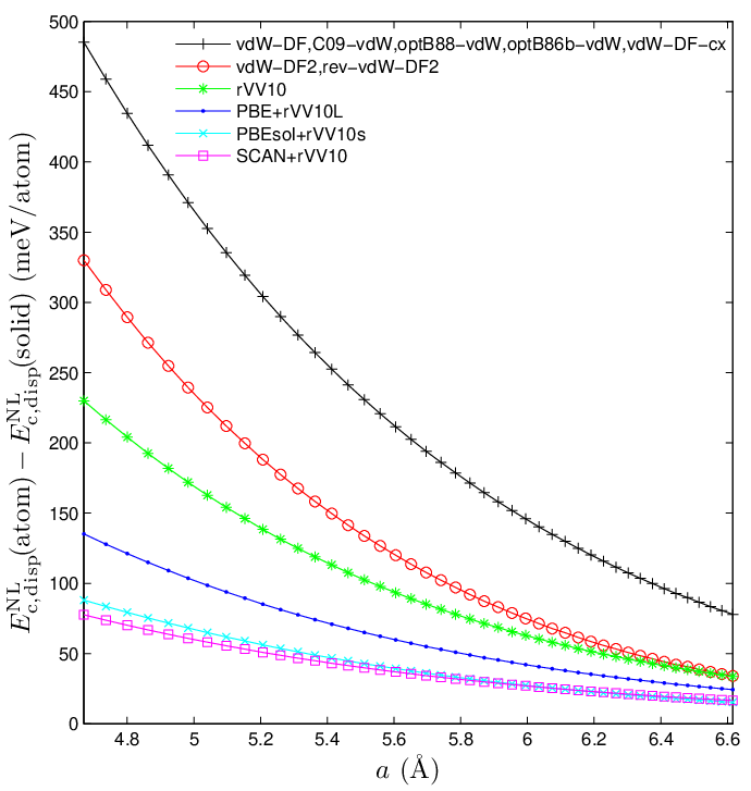
All six variants of the nonlocal dispersion term [Eq. (2)] considered in this work are compared in Fig. (2) which shows the contribution to the cohesive energy of solid Ar (positive values correspond to binding). Since represents mainly the dispersion, which is attractive, the curves in Fig. (2) are positive (stronger bonding) and have a negative slope (which favors shorter bond lengths). It can be seen that the magnitude varies dramatically among the different expressions for Eq. (2). The original DRSLL kernel , that is used in five of the functionals, leads to a contribution to that is the largest and one order of magnitude larger than with the two rVV10-type kernels used in PBEsol+rVV10s and SCAN+rVV10. Since the curve with the steepest slope is also obtained with the DRSLL kernel, then the effect on the bond length should also be the largest when using this kernel. We mention that the ordering of the curves observed for Ar should remain the same for all or at least most other systems.
The calculations on periodic solids were done with the WIEN2k code,Blaha et al. 2018 which is a full-potential and all-electron code based on the linearized augmented plane-wave method.Andersen 1975; Singh and Nordström 2006 The implementation of the NL-vdW functionals into WIEN2k has been reported recentlyTran et al. 2017 and uses the RPS methodRomán-Pérez and Soler 2009 to evaluate efficiently the NL dispersion energy [Eq. (2)] and the potential entering into the Kohn-Sham equations. Since the RPS method is based on fast Fourier transforms, it is necessary to smooth the all-electron density around the nuclei, otherwise a plane-wave expansion of in the whole unit cell would be practically impossible. The smooth density that is used for the RPS method is given by
| (5) |
where bohr3 and is the density cutoff that determines the degree of smoothness applied to . As discussed in detail in Ref. Tran et al. 2017, has to be chosen low enough so that the plane-wave expansion of is small enough to avoid too expensive fast Fourier transforms. On the other hand, should also not be too low, otherwise some accuracy with respect to the calculation with the original density may be lost.
We mention that the WIEN2k calculations with the DRSLL and LMKLL kernels presented in this work (but not those in our previous workTran et al. 2017) were obtained with the version of these kernels generalized for spin-polarized systems,Thonhauser et al. 2015 which is relevant for the calculations of the cohesive energyGharaee et al. 2017 (most atoms are spin-polarized) and for bulk Ni which is ferromagnetic. In such spin-polarized cases, Eq. (5) is first applied to the total density , then the smooth spin- densities are obtained by multiplying by : . The calculations with the functionals of the rVV10-family were done with the non-spin-polarized version of the kernel, since apparently no spin-polarized version has been proposed or used (in particular, the implementation of the rVV10 kernel in the Quantum ESPRESSOSabatini et al. 2013; Giannozzi et al. 2017 code is non-spin polarized).
The usual parameters, like the size of the basis set or the number of -points for the integrations in the Brillouin zone, were chosen such that the results are well converged. As in our previous works,Tran et al. 2016; Tran et al. 2018; Kovács et al. 2019 the results for the strongly bound solids were obtained non-self-consistently using the PBE orbitals and density, however the self-consistent effects are in general quite small, below 0.005 Å in most cases (the optB88-vdW results from the present work can be compared to those obtained self-consistently in Ref. Tran et al. 2017). The calculations on the weakly bound solids were done self-consistently, except those obtained with MGGA functionals (SCAN, SCAN+rVV10, and TM) that were done non-self-consistently using the PBE orbitals and density since the potential of MGGA functionals is not implemented in WIEN2k.
| Strongly bound solids |
| C (), Si (), Ge (), Sn (), |
| SiC (), BN (), BP (), AlN (), |
| AlP (), AlAs (), GaN (), GaP(), |
| GaAs (), InP (), InAs (), InSb (), |
| LiH (), LiF (), LiCl (), NaF (), |
| NaCl (), MgO (), Li (), Na (), |
| Al (), K (), Ca (), Rb (), |
| Sr (), Cs (), Ba (), V (), |
| Ni (), Cu (), Nb (), Mo (), |
| Rh (), Pd (), Ag (), Ta (), |
| W (), Ir (), Pt (), Au () |
| Weakly bound solids |
| Rare gases: Ne (), Ar (), Kr (), |
| Xe () |
| Layered solids: graphite (), h-BN (), |
| TiS2 (), TiSe2 (), MoS2 (), |
| MoSe2 (), MoTe2 (), |
| HfTe2 (), WS2 (), WSe2 () |
| Molecular solids: NH3 (), CO2 (), |
| C6H12N4 () |
The list of solids composing our test set can be found in Table 1 along with their space group. This set consists of 44 solids with (relatively) strong bonding of the metallic, ionic, or covalent type, and 17 solids with weak noncovalent bonding. The strongly bound, rare-gas, and molecular solids have a cubic cell, while the structure of the layered solids are based on the stacking of hexagonal layers. The reference values for the lattice constants and binding energies, to which the DFT values will be compared in Sec. III, were obtained either from experiment or from accurate ab initio methods. Most of these values, except those for the lattice constant of the molecular solids, are corrected for the thermal and zero-point vibrational effects, such that a direct comparison with our DFT values is possible.
As already mentioned, results for the atomization energy of molecules will also be shown. Our test set is the AE6 set of six molecules (SiH4, SiO, S2, C3H4, C2H2O2, C4H8), which were selected to give a fair idea of the accuracy of quantum chemistry methods.Lynch and Truhlar 2003 Most of the calculations were obtained with the Gaussian augmented plane-wave method as implemented in the CP2K code,VandeVondele et al. 2005 which allows calculations with NL-vdW functionals.Tran and Hutter 2013 However, since not all functionals are available in CP2K, calculations were also done with the VASPKresse and Furthmüller 1996 (based on the projector augmented wave methodBlöchl 1994) and deMon (using Gaussian basis functions) codes.Casida et al. 1998 We mention that the spin-polarized versions of the DRSLL and LMKLL kernels are not available in the CP2K and VASP codes, therefore the calculations were done with the spin-unpolarized form of the kernels. However, the results were then approximately corrected by adding the spin correction (the difference between the spin- and non-spin-polarized versions of ) calculated with the WIEN2k code. Furthermore, since many of our results obtained with NL-vdW functionals for the AE6 test set strongly disagree with those presented in Ref. Callsen and Hamada 2015, the VASP results were also used to cross-check the CP2K results (alternatively, WIEN2k could have been used for this purpose).
To finish, we mention that Libxc, a library of exchange-correlation functionals,Marques et al. 2012; Lehtola et al. 2018 has been used for some of the calculations done with the CP2K and WIEN2k codes.
III Results and discussion
III.1 Strongly bound solids
| Method | ME | MAE | MRE | MARE | MAXRE | ME | MAE | MRE | MARE | MAXRE | ME | MAE | MRE | MARE | MAXRE |
|---|---|---|---|---|---|---|---|---|---|---|---|---|---|---|---|
| Without dispersion | |||||||||||||||
| TM | -1.8 (Na) | 25.2 (Cu) | 26.8 (Cu) | ||||||||||||
| SCAN | 3.8 (Cs) | -22.0 (Rb) | -16.6 (Cs) | ||||||||||||
| PBEsol | -2.3 (Sr) | 19.5 (Ni) | 22.8 (Ni) | ||||||||||||
| PBE | 2.8 (Sn) | -25.5 (Ge) | -21.0 (Au) | ||||||||||||
| LDA | -4.9 (Ba) | 32.8 (Ni) | 38.7 (Ni) | ||||||||||||
| With dispersion | |||||||||||||||
| SCAN+rVV10 | 2.5 (Cs) | 22.9 (Cu) | 17.6 (Cu) | ||||||||||||
| PBEsol+rVV10s | -3.0 (Ba) | 22.8 (Ni) | 27.7 (Ni) | ||||||||||||
| C09-vdW | -3.2 (Ba) | 18.2 (V) | 20.2 (Ni) | ||||||||||||
| vdW-DF-cx | -2.5 (Ba) | -18.9 (NaF) | 16.8 (Ir) | ||||||||||||
| PBE-D3(BJ) | -3.1 (Li) | -22.6 (Ge) | 15.7 (Ni) | ||||||||||||
| optB86b-vdW | -2.2 (Sr) | -21.5 (Ge) | 13.6 (Ir) | ||||||||||||
| PBE+rVV10L | 2.1 (Sn) | -21.6 (Ge) | 13.1 (Ni) | ||||||||||||
| rev-vdW-DF2 | -2.1 (Sr) | -23.6 (Ge) | -12.3 (Rb) | ||||||||||||
| revPBE-D3(BJ) | -4.8 (Li) | -23.2 (Ge) | 18.7 (Cu) | ||||||||||||
| optB88-vdW | -2.8 (Cs) | -26.3 (Ge) | -13.4 (Na) | ||||||||||||
| rVV10 | 3.4 (Au) | -29.8 (Ge) | 10.4 (Ba) | ||||||||||||
| vdW-DF | 4.6 (Au) | -43.0 (Au) | -32.4 (Au) | ||||||||||||
| vdW-DF2 | 6.9 (Au) | -51.7 (Au) | -35.4 (Sr) | ||||||||||||


The results for the equilibrium lattice constant , bulk modulus , and cohesive energy of strongly bound solids obtained with the tested xc-functionals are shown in Table 2. ME, MAE, MRE, and MARE represent the mean values of the error, absolute error, relative error, and absolute relative error with respect to experiment, respectively, while MAXRE is the maximum relative error. The experimental values were corrected for thermal and zero-point vibrational effects.Schimka et al. 2011; Lejaeghere et al. 2014 For a few selected functionals, Figs. 3 and 4 show graphically the errors. All detailed results are available in Tables S1-S9 and shown graphically in Figs. S1-S18 of Ref. SM_.
For the lattice constant, the NL-vdW MGGA SCAN+rVV10 and MGGA TM lead to the lowest MAE (0.02 Å) and MARE (0.5%). Without the nonlocal dispersion term, the MAE and MARE with SCAN only slightly increases to 0.03 Å and 0.6%, which are the same values obtained with the GGA PBEsol. Note that other accurate GGA functionals like SG4Constantin et al. 2016 or WCWu and Cohen 2006 also lead to errors in this range (see Ref. Tran et al. 2016). Interestingly, the ME and MRE for SCAN+rVV10 are basically zero, which means that this functional does not show a particular tendency towards underestimation or overestimation of . Most of the other modern functionals lead to values that are in the range 0.04-0.05 Å for the MAE and 0.8-1.0% for the MARE. The results obtained with the recent PBEsol+rVV10s can be considered as very accurate and are overall only slightly deteriorated with respect to those obtained with the GGA PBEsol without dispersion correction. As already known from previous studies (see, e.g., Refs. Klimeš et al. 2011; Park et al. 2015), the first two original NL-vdW functionals vdW-DF and vdW-DF2 lead to very large overestimations, similarly as the worst GGAs for solids like BLYPBecke 1988; Lee et al. 1988 do.Tran et al. 2016 This is due to the strong magnitude of the enhancement factors of the corresponding semilocal components (see Fig. 1) which favor too much inhomogeneities in , and therefore too large equilibrium volumes, in the case of solids. rVV10 also shows a clear overestimation of the lattice constant which is nearly as large as with PBE. From Fig. 1, we can see that the factor is slightly larger in the case of rVV10 than PBE, however the additional nonlocal term in rVV10 reduces the overestimation in .
As expected, the accuracy for the bulk modulus follows a trend that is rather similar as for the lattice constant; if a functional is among the most accurate for , then the same conclusion holds also for .
The results for the cohesive energy show that the lowest MAE (0.13 eV/atom) and MARE (%) are obtained with the NL-vdW functional rVV10. Remarkably, these mean errors are smaller than all those obtained with the 62 functionals tested in Ref. Tran et al. 2016. However, the price to pay is to have errors for the lattice constant that are quite large, since the MAE and MARE are more than three times larger than with SCAN+rVV10. Actually, this is a problem that is often encountered with GGAs: a functional that is among the most accurate ones for property A will most likely not be very accurate for another property B that is quite different from property A (see also Sec. III.3). Also very accurate are optB88-vdW and rev-vdW-DF2 with MAE of 0.13-0.14 eV/atom and MARE in the range 3.8-4.0%. The results obtained with SCAN+rVV10 (the best one for ) are relatively fair, but a certain number of other functionals perform better. We also note the extremely bad performance (strong overestimation) of PBEsol+rVV10s for with MAE and MARE of 0.45 eV/atom and 10.6%, respectively, which makes this functional the fourth worst after LDA, vdW-DF2, and vdW-DF. Actually, as expected and already shown in Ref. Terentjev et al. 2018a PBEsol+rVV10s significantly worsens the cohesive energy with respect to PBEsol, while it was only slightly the case for the lattice constant.
By considering the results in Table 2 as a whole, an accurate or satisfying description of the three properties seems to be achieved by the following functionals: SCAN, SCAN+rVV10, vdW-DF-cx, PBE-D3(BJ), optB86b-vdW, PBE+rVV10L, and rev-vdW-DF2,
Figures 3 and 4 show the results for the lattice constant and cohesive energy for some of the most recent NL-vdW functionals as well as the MGGAs SCAN and TM. A few interesting observations are the following. The underestimation (overestimation) by PBEsol+rVV10s of the lattice constant (cohesive energy) is particularly pronounced for the alkali and alkaline earth metals. For some of the transition metals, namely Ni, Cu, Rh, Pd, and Ir, PBEsol+rVV10s and TM clearly overestimate . Interestingly, for the lattice constant, PBE+rVV10L and rev-vdW-DF2 lead to very similar results except for the heavy alkali and alkaline earth metals. We note that in general, the difference between the SCAN and SCAN+rVV10 results is quite small, which can be inferred from Fig. 1, where we already observed that the NL-vdW term of SCAN+rVV10 has the smallest magnitude. Finally, we mention that SCAN+rVV10 does not perform well for Cs (strong overestimation of ), but leads to rather consistent results for the semiconductors and the transition metals.
III.2 Weakly bound solids
III.2.1 Rare-gas solids
| Method | Ne | Ar | Kr | Xe | ME | MAE | MRE | MARE |
|---|---|---|---|---|---|---|---|---|
| Without dispersion | ||||||||
| TM | 4.05 (-6) | 5.23 (0) | 5.60 (0) | 6.15 (1) | -0.05 | 0.08 | -1.2 | 1.8 |
| SCAN | 4.03 (-6) | 5.31 (1) | 5.74 (2) | 6.33 (4) | 0.04 | 0.18 | 0.3 | 3.4 |
| LDA | 3.86 (-10) | 4.94 (-6) | 5.33 (-5) | 5.85 (-4) | -0.31 | 0.31 | -6.2 | 6.2 |
| PBEsol | 4.70 (9) | 5.88 (12) | 6.13 (10) | 6.48 (6) | 0.49 | 0.49 | 9.3 | 9.3 |
| PBE | 4.60 (7) | 5.96 (13) | 6.42 (15) | 7.03 (16) | 0.69 | 0.69 | 12.7 | 12.7 |
| With dispersion | ||||||||
| optB88-vdW | 4.26 (-1) | 5.23 (0) | 5.63 (1) | 6.15 (1) | 0.01 | 0.04 | 0.1 | 0.7 |
| optB86b-vdW | 4.35 (1) | 5.32 (1) | 5.68 (1) | 6.18 (2) | 0.07 | 0.07 | 1.4 | 1.4 |
| rVV10 | 4.21 (-2) | 5.16 (-2) | 5.52 (-1) | 6.01 (-1) | -0.08 | 0.08 | -1.6 | 1.6 |
| PBEsol+rVV10s | 4.41 (3) | 5.38 (2) | 5.67 (1) | 6.08 (0) | 0.08 | 0.08 | 1.6 | 1.6 |
| C09-vdW | 4.55 (6) | 5.34 (2) | 5.63 (1) | 6.07 (0) | 0.09 | 0.10 | 2.0 | 2.1 |
| vdW-DF2 | 4.17 (-3) | 5.28 (1) | 5.74 (2) | 6.31 (4) | 0.07 | 0.13 | 1.0 | 2.4 |
| rev-vdW-DF2 | 4.42 (3) | 5.37 (2) | 5.74 (3) | 6.22 (2) | 0.13 | 0.13 | 2.5 | 2.5 |
| SCAN+rVV10 | 3.97 (-8) | 5.17 (-1) | 5.56 (-1) | 6.12 (1) | -0.10 | 0.12 | -2.3 | 2.6 |
| PBE+rVV10L | 4.37 (2) | 5.48 (4) | 5.86 (5) | 6.33 (4) | 0.20 | 0.20 | 3.6 | 3.6 |
| PBE-D3(BJ) | 4.46 (4) | 5.49 (5) | 5.85 (5) | 6.31 (4) | 0.22 | 0.22 | 4.1 | 4.1 |
| vdW-DF | 4.34 (1) | 5.50 (5) | 5.95 (6) | 6.54 (7) | 0.28 | 0.28 | 4.9 | 4.9 |
| vdW-DF-cx | 4.40 (2) | 5.59 (7) | 6.05 (8) | 6.53 (7) | 0.34 | 0.34 | 6.1 | 6.1 |
| revPBE-D3(BJ) | 4.80 (12) | 5.67 (8) | 5.96 (7) | 6.37 (5) | 0.39 | 0.39 | 7.8 | 7.8 |
| Reference11 1 The set of CCSD(T) results from Ref. Rościszewski et al. 2000 that include the two-, three-, and four-body contributions, but not the effect due to the zero-point vibration. | 4.30 | 5.25 | 5.60 | 6.09 | ||||
| Without dispersion | ||||||||
| TM | 47 (80) | 62 (-30) | 82 (-33) | 95 (-44) | -30 | 41 | -6.7 | 46.6 |
| SCAN | 54 (107) | 61 (-30) | 72 (-41) | 74 (-56) | -36 | 50 | -5.2 | 58.7 |
| PBE | 19 (-26) | 23 (-73) | 27 (-78) | 29 (-83) | -77 | 77 | -64.9 | 64.9 |
| PBEsol | 12 (-54) | 17 (-81) | 23 (-81) | 32 (-81) | -81 | 81 | -74.4 | 74.4 |
| LDA | 87 (234) | 138 (57) | 169 (39) | 202 (19) | 48 | 48 | 87.2 | 87.2 |
| With dispersion | ||||||||
| revPBE-D3(BJ) | 25 (-2) | 82 (-7) | 126 (3) | 192 (13) | 5 | 8 | 1.7 | 6.5 |
| rev-vdW-DF2 | 31 (19) | 82 (-7) | 111 (-9) | 148 (-13) | -9 | 11 | -2.4 | 12.0 |
| PBE-D3(BJ) | 37 (42) | 86 (-2) | 117 (-4) | 162 (-5) | -1 | 6 | 7.6 | 13.1 |
| PBEsol+rVV10s | 29 (10) | 57 (-35) | 75 (-39) | 111 (-35) | -34 | 35 | -24.7 | 29.8 |
| PBE+rVV10L | 45 (72) | 79 (-10) | 102 (-17) | 130 (-24) | -13 | 22 | 5.4 | 30.7 |
| rVV10 | 42 (60) | 113 (28) | 162 (33) | 226 (33) | 34 | 34 | 38.4 | 38.4 |
| C09-vdW | 51 (98) | 118 (34) | 156 (28) | 212 (25) | 33 | 33 | 46.1 | 46.1 |
| vdW-DF2 | 58 (122) | 124 (41) | 154 (27) | 190 (11) | 30 | 30 | 50.0 | 50.0 |
| optB88-vdW | 50 (93) | 138 (57) | 180 (47) | 234 (37) | 49 | 49 | 58.7 | 58.7 |
| SCAN+rVV10 | 79 (204) | 111 (26) | 137 (12) | 159 (-7) | 20 | 26 | 58.9 | 62.3 |
| optB86b-vdW | 61 (134) | 137 (56) | 174 (42) | 224 (32) | 47 | 47 | 65.9 | 65.9 |
| vdW-DF-cx | 79 (205) | 137 (56) | 160 (31) | 191 (12) | 40 | 40 | 76.0 | 76.0 |
| vdW-DF | 92 (253) | 156 (77) | 181 (49) | 212 (25) | 59 | 59 | 100.9 | 100.9 |
| Reference11 1 The set of CCSD(T) results from Ref. Rościszewski et al. 2000 that include the two-, three-, and four-body contributions, but not the effect due to the zero-point vibration. | 26 | 88 | 122 | 170 | ||||
Turning to weakly bound systems, Table 3 shows the results for the rare-gas solids Ne, Ar, Kr, and Xe which crystallize in the face-centered cubic structure and have been used in many previous works Ortmann et al. 2006; Tran et al. 2007; Harl and Kresse 2008; Haas et al. 2009; Yousaf and Brothers 2010; Bučko et al. 2010; Al-Saidi et al. 2012; Bučko et al. 2013a; Tran and Hutter 2013; Moellmann and Grimme 2014; Callsen and Hamada 2015; Tran et al. 2016; Peng et al. 2016; Terentjev et al. 2018b; Tran et al. 2018; Terentjev et al. 2018a for testing functionals since they represent the prototypical van der Waals systems bound by dispersion forces. As criteria to decide what is an (unacceptably) large error with respect to the very accurate CCSD(T) (coupled cluster with singlet, doublet, and perturbative triplet) values,Rościszewski et al. 2000 we chose 5% and 30% for the relative error on the lattice constant and cohesive energy, respectively.
The results show that only one method, the NL-vdW functional rev-vdW-DF2, leads to no such large errors as defined by our criteria (see also Ref. Callsen and Hamada 2015). The largest error is 3% for (Ne and Kr) and 19% for (Ne). Another functional which also performs rather well and shows only one large error is the atom-pairwise PBE-D3(BJ), which leads to an overestimation of 42% for of Ne, but below 5% for the others. The other atom-pairwise functional, revPBE-D3(BJ), leads to very accurate cohesive energy for the four rare gases, but is overall one of the most inaccurate methods for the lattice constant. Somehow satisfying overall, PBEsol+rVV10s leads to errors in the range 35-40% for the cohesive energy of Ar, Kr, and Xe, but only 10% for Ne.
All other functionals lead to at least one very large error above 50% for , including SCAN+rVV10 that performs very badly for Ne for both and , as already noticed in Ref. Peng et al. 2016. Thus, except rev-vdW-DF2, PBE-D3(BJ), and PBEsol+rVV10s, none of the other functionals can be considered as satisfying for rare-gas solids. However, note that other non-hybrid DFT+D3 or DFT+D3(BJ) methods, e.g. PBEsol-D3(BJ)Goerigk and Grimme 2011 or BLYP-D3,Grimme et al. 2010 can also be reliable for the rare gases, as shown in our previous work.Tran et al. 2016 We can also see that the most accurate methods for , optB88-vdW and optB86b-vdW, which lead to errors not larger than are extremely inaccurate for in all cases.
III.2.2 Layered solids
| Method | Graphite | h-BN | TiS2 | TiSe2 | MoS2 | MoSe2 | MoTe2 | HfTe2 | WS2 | WSe2 | ME | MAE | MRE | MARE |
|---|---|---|---|---|---|---|---|---|---|---|---|---|---|---|
| Without dispersion | ||||||||||||||
| SCAN | 2.45 (0) | 2.50 (0) | 3.42 (0) | 3.54 (0) | 3.18 (1) | 3.30 (0) | 3.53 (0) | 3.97 (0) | 3.17 (1) | 3.30 (1) | 0.01 | 0.01 | 0.2 | 0.4 |
| TM | 2.46 (0) | 2.51 (0) | 3.38 (-1) | 3.50 (-1) | 3.15 (0) | 3.27 (-1) | 3.49 (-1) | 3.90 (-1) | 3.15 (0) | 3.27 (0) | -0.02 | 0.02 | -0.5 | 0.6 |
| PBE | 2.47 (1) | 2.51 (0) | 3.42 (0) | 3.54 (0) | 3.19 (1) | 3.32 (1) | 3.56 (1) | 3.98 (1) | 3.19 (1) | 3.32 (1) | 0.02 | 0.02 | 0.7 | 0.7 |
| PBEsol | 2.46 (0) | 2.50 (0) | 3.35 (-2) | 3.48 (-2) | 3.14 (-1) | 3.27 (-1) | 3.50 (-1) | 3.88 (-2) | 3.15 (0) | 3.27 (0) | -0.03 | 0.03 | -0.8 | 0.8 |
| LDA | 2.45 (0) | 2.49 (-1) | 3.31 (-3) | 3.43 (-3) | 3.12 (-1) | 3.25 (-1) | 3.47 (-1) | 3.82 (-3) | 3.13 (-1) | 3.25 (-1) | -0.06 | 0.06 | -1.6 | 1.6 |
| With dispersion | ||||||||||||||
| SCAN+rVV10 | 2.45 (0) | 2.50 (0) | 3.41 (0) | 3.54 (0) | 3.17 (0) | 3.29 (0) | 3.52 (0) | 3.95 (0) | 3.16 (0) | 3.29 (0) | 0.00 | 0.01 | 0.0 | 0.2 |
| PBE+rVV10L | 2.46 (0) | 2.51 (0) | 3.39 (-1) | 3.52 (0) | 3.17 (0) | 3.30 (0) | 3.53 (0) | 3.94 (0) | 3.17 (1) | 3.30 (1) | 0.00 | 0.01 | 0.1 | 0.4 |
| optB86b-vdW | 2.46 (0) | 2.51 (0) | 3.38 (-1) | 3.52 (0) | 3.17 (0) | 3.30 (0) | 3.53 (0) | 3.94 (0) | 3.17 (1) | 3.30 (1) | 0.00 | 0.01 | 0.0 | 0.4 |
| rev-vdW-DF2 | 2.46 (0) | 2.51 (0) | 3.39 (-1) | 3.52 (0) | 3.17 (0) | 3.31 (1) | 3.54 (1) | 3.95 (0) | 3.17 (1) | 3.30 (1) | 0.00 | 0.01 | 0.2 | 0.4 |
| vdW-DF-cx | 2.46 (0) | 2.51 (0) | 3.36 (-1) | 3.49 (-1) | 3.15 (0) | 3.28 (0) | 3.51 (0) | 3.90 (-1) | 3.15 (0) | 3.28 (0) | -0.02 | 0.02 | -0.5 | 0.5 |
| PBE-D3(BJ) | 2.46 (0) | 2.51 (0) | 3.36 (-1) | 3.49 (-1) | 3.16 (0) | 3.28 (0) | 3.50 (-1) | 3.90 (-1) | 3.19 (1) | 3.29 (0) | -0.01 | 0.02 | -0.3 | 0.7 |
| optB88-vdW | 2.46 (0) | 2.51 (0) | 3.41 (0) | 3.55 (0) | 3.19 (1) | 3.32 (1) | 3.58 (2) | 3.99 (1) | 3.19 (1) | 3.32 (1) | 0.02 | 0.02 | 0.7 | 0.7 |
| C09-vdW | 2.46 (0) | 2.51 (0) | 3.35 (-2) | 3.48 (-2) | 3.14 (-1) | 3.27 (-1) | 3.49 (-1) | 3.88 (-2) | 3.15 (0) | 3.27 (0) | -0.03 | 0.03 | -0.8 | 0.8 |
| revPBE-D3(BJ) | 2.47 (1) | 2.51 (0) | 3.34 (-2) | 3.46 (-2) | 3.13 (-1) | 3.25 (-1) | 3.47 (-1) | 3.85 (-3) | 3.14 (0) | 3.26 (-1) | -0.04 | 0.04 | -1.1 | 1.2 |
| PBEsol+rVV10s | 2.46 (0) | 2.50 (0) | 3.33 (-2) | 3.46 (-2) | 3.13 (-1) | 3.25 (-1) | 3.47 (-1) | 3.83 (-3) | 3.13 (-1) | 3.26 (-1) | -0.05 | 0.05 | -1.3 | 1.3 |
| rVV10 | 2.47 (1) | 2.52 (0) | 3.44 (1) | 3.58 (1) | 3.22 (2) | 3.36 (2) | 3.60 (2) | 4.02 (2) | 3.22 (2) | 3.36 (2) | 0.05 | 0.05 | 1.6 | 1.6 |
| vdW-DF | 2.48 (1) | 2.52 (0) | 3.48 (2) | 3.62 (2) | 3.24 (2) | 3.38 (3) | 3.64 (3) | 4.08 (3) | 3.24 (3) | 3.38 (3) | 0.08 | 0.08 | 2.3 | 2.3 |
| vdW-DF2 | 2.48 (1) | 2.52 (0) | 3.52 (3) | 3.68 (4) | 3.29 (4) | 3.45 (5) | 3.72 (6) | 4.16 (5) | 3.29 (4) | 3.44 (5) | 0.13 | 0.13 | 3.8 | 3.8 |
| Reference | 2.46 | 2.51 | 3.41 | 3.54 | 3.16 | 3.29 | 3.52 | 3.96 | 3.15 | 3.28 | ||||
| Without dispersion | ||||||||||||||
| TM | 6.63 (0) | 6.51 (-2) | 5.76 (1) | 6.12 (2) | 12.5 (2) | 13.2 (2) | 14.2 (2) | 6.75 (2) | 12.6 (2) | 13.2 (2) | 0.2 | 0.2 | 1.4 | 1.7 |
| LDA | 6.63 (0) | 6.49 (-2) | 5.45 (-4) | 5.80 (-3) | 12.1 (-2) | 12.8 (-1) | 13.8 (-1) | 6.50 (-2) | 12.2 (-1) | 12.8 (-1) | -0.2 | 0.2 | -1.8 | 1.8 |
| PBEsol | 7.26 (9) | 7.06 (6) | 5.65 (-1) | 5.92 (-1) | 12.6 (3) | 13.1 (2) | 14.0 (0) | 6.60 (-1) | 12.7 (3) | 13.2 (2) | 0.2 | 0.2 | 2.3 | 2.9 |
| SCAN | 6.95 (5) | 6.82 (3) | 5.93 (4) | 6.32 (5) | 12.9 (5) | 13.6 (5) | 14.7 (5) | 6.97 (5) | 12.9 (5) | 13.6 (5) | 0.5 | 0.5 | 4.8 | 4.8 |
| PBE | 8.84 (33) | 8.69 (31) | 6.61 (16) | 6.70 (12) | 14.8 (21) | 15.1 (17) | 15.3 (10) | 7.21 (9) | 14.9 (21) | 15.2 (18) | 1.7 | 1.7 | 18.7 | 18.7 |
| With dispersion | ||||||||||||||
| rev-vdW-DF2 | 6.64 (0) | 6.57 (-1) | 5.68 (0) | 6.00 (0) | 12.4 (1) | 13.1 (1) | 14.1 (1) | 6.71 (1) | 12.4 (1) | 13.2 (2) | 0.1 | 0.1 | 0.6 | 0.9 |
| optB86b-vdW | 6.63 (0) | 6.53 (-2) | 5.69 (0) | 6.00 (0) | 12.4 (1) | 13.1 (1) | 14.1 (1) | 6.70 (1) | 12.5 (1) | 13.2 (2) | 0.1 | 0.1 | 0.5 | 0.9 |
| vdW-DF-cx | 6.56 (-1) | 6.45 (-3) | 5.61 (-2) | 5.93 (-1) | 12.3 (0) | 12.9 (0) | 13.9 (0) | 6.60 (-1) | 12.4 (1) | 13.0 (1) | -0.0 | 0.1 | -0.6 | 0.9 |
| PBEsol+rVV10s | 6.70 (1) | 6.60 (-1) | 5.54 (-3) | 5.87 (-2) | 12.2 (-1) | 12.9 (0) | 13.8 (-1) | 6.57 (-1) | 12.3 (0) | 13.0 (0) | -0.1 | 0.1 | -0.7 | 0.9 |
| rVV10 | 6.71 (1) | 6.62 (0) | 5.70 (0) | 6.05 (1) | 12.4 (1) | 13.1 (2) | 14.2 (2) | 6.75 (2) | 12.5 (1) | 13.2 (2) | 0.1 | 0.1 | 1.1 | 1.1 |
| C09-vdW | 6.46 (-3) | 6.35 (-4) | 5.55 (-3) | 5.89 (-2) | 12.2 (-1) | 12.8 (0) | 13.9 (-1) | 6.57 (-1) | 12.2 (0) | 12.9 (0) | -0.1 | 0.1 | -1.5 | 1.5 |
| PBE-D3(BJ) | 6.79 (2) | 6.68 (1) | 5.56 (-2) | 5.59 (-7) | 12.2 (-1) | 12.8 (0) | 13.8 (-1) | 6.58 (-1) | 12.2 (0) | 12.9 (0) | -0.1 | 0.1 | -1.0 | 1.6 |
| optB88-vdW | 6.69 (1) | 6.60 (-1) | 5.75 (1) | 6.14 (2) | 12.5 (2) | 13.2 (2) | 14.3 (2) | 6.80 (2) | 12.6 (2) | 13.3 (2) | 0.2 | 0.2 | 1.7 | 1.8 |
| SCAN+rVV10 | 6.68 (1) | 6.59 (-1) | 5.75 (1) | 6.22 (4) | 12.5 (1) | 13.2 (2) | 14.3 (2) | 6.82 (3) | 12.6 (2) | 13.2 (2) | 0.2 | 0.2 | 1.8 | 1.9 |
| PBE+rVV10L | 6.98 (5) | 6.88 (4) | 5.78 (1) | 6.04 (1) | 12.6 (2) | 13.2 (2) | 14.1 (1) | 6.71 (1) | 12.7 (3) | 13.2 (2) | 0.2 | 0.2 | 2.3 | 2.3 |
| revPBE-D3(BJ) | 6.45 (-3) | 6.34 (-4) | 5.40 (-5) | 5.76 (-4) | 11.8 (-4) | 12.5 (-3) | 13.5 (-3) | 6.50 (-2) | 11.8 (-4) | 12.5 (-3) | -0.3 | 0.3 | -3.6 | 3.6 |
| vdW-DF2 | 7.06 (6) | 6.99 (5) | 5.96 (5) | 6.36 (6) | 12.9 (5) | 13.7 (6) | 14.9 (7) | 7.07 (6) | 13.0 (5) | 13.7 (6) | 0.6 | 0.6 | 5.8 | 5.8 |
| vdW-DF | 7.19 (8) | 7.12 (7) | 6.11 (7) | 6.50 (8) | 13.2 (7) | 13.9 (7) | 15.0 (8) | 7.18 (8) | 13.2 (7) | 13.9 (8) | 0.7 | 0.7 | 7.7 | 7.7 |
| Reference | 6.63 | 6.63 | 5.70 | 6.00 | 12.28 | 12.91 | 13.96 | 6.64 | 12.31 | 12.95 | ||||
| Without dispersion | ||||||||||||||
| LDA | 10 (-48) | 10 (-30) | 20 (7) | 21 (24) | 13 (-35) | 14 (-29) | 15 (-26) | 19 (3) | 13 (-37) | 13 (-32) | -4 | 5 | -20.4 | 27.4 |
| TM | 11 (-38) | 12 (-19) | 13 (-31) | 14 (-19) | 10 (-50) | 11 (-42) | 13 (-36) | 13 (-28) | 10 (-50) | 11 (-44) | -7 | 7 | -35.7 | 35.7 |
| SCAN | 7 (-59) | 8 (-45) | 6 (-68) | 6 (-64) | 6 (-73) | 5 (-72) | 7 (-65) | 7 (-60) | 6 (-72) | 5 (-73) | -12 | 12 | -65.2 | 65.2 |
| PBEsol | 2 (-92) | 2 (-86) | 7 (-62) | 10 (-44) | 3 (-84) | 5 (-75) | 8 (-62) | 10 (-45) | 3 (-86) | 4 (-77) | -13 | 13 | -71.4 | 71.4 |
| PBE | 1 (-97) | 1 (-96) | 1 (-93) | 2 (-90) | 1 (-97) | 1 (-97) | 1 (-94) | 2 (-90) | 1 (-97) | 1 (-97) | -18 | 18 | -94.8 | 94.8 |
| With dispersion | ||||||||||||||
| SCAN+rVV10 | 20 (7) | 19 (34) | 18 (-3) | 18 (3) | 20 (-3) | 19 (-1) | 21 (2) | 19 (0) | 21 (4) | 20 (-1) | 1 | 1 | 4.3 | 5.8 |
| PBE+rVV10L | 15 (-19) | 14 (-4) | 19 (2) | 20 (18) | 19 (-6) | 20 (2) | 22 (4) | 20 (6) | 19 (-5) | 20 (1) | -0 | 1 | -0.1 | 6.7 |
| vdW-DF2 | 20 (8) | 19 (29) | 19 (1) | 18 (2) | 19 (-6) | 18 (-9) | 16 (-21) | 15 (-19) | 19 (-5) | 18 (-10) | -1 | 2 | -3.0 | 10.9 |
| vdW-DF | 20 (12) | 19 (35) | 19 (0) | 18 (2) | 19 (-7) | 18 (-10) | 16 (-21) | 15 (-18) | 19 (-5) | 18 (-11) | -1 | 2 | -2.3 | 12.0 |
| PBEsol+rVV10s | 12 (-32) | 12 (-20) | 20 (7) | 21 (21) | 17 (-15) | 17 (-11) | 21 (3) | 22 (19) | 17 (-14) | 17 (-12) | -1 | 3 | -5.4 | 15.3 |
| rev-vdW-DF2 | 23 (23) | 21 (47) | 25 (30) | 24 (40) | 23 (14) | 22 (15) | 23 (9) | 22 (16) | 23 (14) | 22 (12) | 4 | 4 | 22.0 | 22.0 |
| PBE-D3(BJ) | 17 (-9) | 16 (9) | 27 (45) | 30 (72) | 24 (17) | 26 (34) | 30 (44) | 27 (46) | 26 (28) | 28 (38) | 6 | 7 | 32.5 | 34.2 |
| vdW-DF-cx | 25 (36) | 24 (67) | 27 (43) | 27 (59) | 25 (21) | 25 (26) | 26 (25) | 25 (35) | 24 (21) | 24 (23) | 6 | 6 | 35.6 | 35.6 |
| optB88-vdW | 27 (47) | 26 (80) | 27 (45) | 26 (52) | 26 (28) | 25 (29) | 24 (16) | 23 (23) | 26 (29) | 25 (27) | 7 | 7 | 37.5 | 37.5 |
| optB86b-vdW | 27 (47) | 26 (80) | 28 (48) | 28 (60) | 26 (29) | 26 (31) | 26 (24) | 25 (33) | 26 (30) | 26 (28) | 7 | 7 | 41.0 | 41.0 |
| rVV10 | 26 (44) | 25 (72) | 28 (48) | 29 (65) | 29 (42) | 29 (50) | 29 (40) | 26 (40) | 29 (44) | 29 (48) | 9 | 9 | 49.2 | 49.2 |
| C09-vdW | 29 (59) | 28 (96) | 32 (72) | 33 (88) | 30 (44) | 29 (49) | 30 (44) | 30 (59) | 29 (44) | 29 (45) | 11 | 11 | 59.9 | 59.9 |
| revPBE-D3(BJ) | 26 (41) | 25 (71) | 48 (153) | 51 (196) | 45 (118) | 49 (152) | 55 (163) | 46 (147) | 50 (147) | 53 (167) | 26 | 26 | 135.5 | 135.5 |
| Reference | 18.3 | 14.4 | 18.8 | 17.3 | 20.5 | 19.6 | 20.8 | 18.6 | 20.2 | 19.9 | ||||

The hexagonal layered solids constitute another set of prototypical systems bound by weak interactions that is often used for assessing functionals. Hasegawa and Nishidate 2004; Ortmann et al. 2006; Hasegawa et al. 2007; Tran et al. 2007; Haas et al. 2009; Björkman et al. 2012; Björkman et al. 2012; Björkman 2012; Björkman 2014; Graziano et al. 2012; Berland and Hyldgaard 2014; Hamada 2014; Bučko et al. 2013a; Rêgo et al. 2015; Tran et al. 2016; Peng et al. 2016; Lebedeva et al. 2017; Peng and Perdew 2017; Terentjev et al. 2018b; Tawfik et al. 2018; Mejia-Rodriguez and Trickey 2018; Mosyagin et al. 2018; Terentjev et al. 2018a These systems consist of hexagonal layers that are bound by weak interactions, while the atoms within a layer are strongly bound. The results for the intralayer and interlayer lattice constants and as well as the interlayer binding energy are shown in Table 4 and compared to results obtained from experiment for and or the random-phase approximation (RPA) for .Björkman 2014
For selected functionals, the results are also compared graphically in Fig. 5. We mention that in the calculation on the monolayer to get , the intralayer lattice constant was also optimized (results not shown). However, we observed that in the vast majority of cases choosing either or for the monolayer has a very small influence, a few tenths of meV/Å2, on .
The trends observed among the functionals for are, as expected, similar to those for the strongly bound solids discussed above. In brief, the largest underestimations (up to a few percents) are due to LDA, revPBE-D3(BJ), PBEsol+rVV10s, and C09-vdW, while vdW-DF2 leads to very large overestimations (up to 6%). vdW-DF and rVV10 also show a clear tendency towards overestimation of (see also Ref. Björkman 2012). All other functionals perform clearly better and, as shown in Fig. 5, the most accurate one is SCAN+rVV10 which leads to errors below 0.01 Å (below 0.5%) for all systems. For the interlayer lattice constant , the functionals, beside PBE which barely binds the layers, that can be identified as more inaccurate than the others are vdW-DF, vdW-DF2, and SCAN, which clearly overestimate , as well as revPBE-D3(BJ) which does the opposite. For these functionals, the error is at least 4% for a certain number of solids. The other functionals lead to errors which are at most 3% for all or most solids.
Thus, overall vdW-DF, vdW-DF2, and revPBE-D3(BJ) perform very poorly for both and . rVV10 is also among the inaccurate methods for , but performs quite well for . As well-known, LDA systematically underestimates the lattice constant, but does it moderately for since the errors are quite small. Most other dispersion-corrected functionals can be considered as satisfying for both lattice constants. Note that in the work of Björkman,Björkman 2014 optB86b-vdW, vdW-DF-cx, and rev-vdW-DF2 were already shown to be accurate for the lattice constants.
As observed above for the rare-gas solids, the relative errors for the interlayer binding energy are much larger than for the lattice constants. By considering 30% of relative error as the largest acceptable value for , the results in Table 4 show that the functionals which have a reasonable accuracy for all solids except possibly one are SCAN+rVV10, PBE+rVV10L, vdW-DF2, vdW-DF, and PBEsol+rVV10s. rev-vdW-DF2 can also be considered as accurate since for only two solids (h-BN and TiSe2) the relative error is above 30%. Note that the parameter in the PBE+rVV10L kernel was tuned in order to reproduce at best the RPA results for , therefore its good performance is hardly surprising. The worst functionals are PBE and revPBE-D3(BJ); PBE gives nearly no binding, while revPBE-D3(BJ) overestimates by more than 100% in most cases. Such huge overestimations obtained with revPBE-D3(BJ) have already been observed in the case of adsorption of benzene on transition-metal surfaces.Reckien et al. 2014 Other very inaccurate functionals are PBEsol, SCAN, C09-vdW, and rVV10 as already shown in Refs. Björkman et al. 2012; Björkman 2014 for the latter two.
By considering all results for the layered solids, the best functionals are PBE+rVV10L, SCAN+rVV10, and rev-vdW-DF2 since they belong to the accurate methods for , , and at the same time. The results with optB88-vdW and vdW-DF-cx can also be considered as fair. Note the curious performances of vdW-DF and vdW-DF2: very accurate for the interlayer binding energy, but the worst for both lattice constants.Björkman et al. 2012 For these two functionals, the large contribution of the NL-vdW term to (see Fig. 2) leads to an appropriate binding energy, but the corresponding slope is not steep enough to shorten the lattice constant sufficiently.
We also mention that among a dozen of dispersion-corrected functionals of various families, Tawfik et al.Tawfik et al. 2018 concluded that SCAN+rVV10 is overall the most accurate one for a set of twelve layered solids (quite similar to our test set). However, PBE+rVV10L and rev-vdW-DF2 were not considered in their work.
Since results on the layered solids were already available in the literature for many of the functionals, it may be interesting to compare some of them with ours. Peng et al.Peng et al. 2016; Peng and Perdew 2017 reported results for rev-vdW-DF2, PBE+rVV10L, and SCAN+rVV10 that were obtained with VASP. For , their results are in good agreement with ours since they differ by at most 0.01 Å. The agreement for is relatively good for rev-vdW-DF2 and PBE+rVV10L since the difference is typically below 0.05 Å. A difference of 0.05 Å should be considered as acceptable for such large lattice constants determined by weak interactions. However, with SCAN+rVV10 the disagreement for is larger (in the range 0.1-0.2 Å), which should be due to self-consistent effects (see discussion in Ref. Tran et al. 2016). Our calculations involving MGGA functionals were done using PBE(+rVV10) for the potential, while those from VASP calculations were probably done self-consistently. The agreement for is good for the three functionals since the discrepancies are below 1 meV/Å2 in all cases. Considering now the results from BjörkmanBjörkman 2014 for six functionals (e.g., rev-vdW-DF2 or optB88-vdW) obtained with VASP, the results are also in fair agreement with ours for the lattice constants. However, sizable discrepancies are observed for , since his results are consistently smaller by 2-3 meV/Å2 compared to our results which agree quite well with those from Peng et al.Peng et al. 2016; Peng and Perdew 2017 and Berland and Hyldgaard.Berland and Hyldgaard 2014
III.2.3 Molecular solids
| NH3 | CO2 | C6H12N4 | ||||
| Method | ||||||
| Without dispersion | ||||||
| TM | 4.98 (-1) | 0.39 (1) | 5.49 (-1) | 0.25 (-15) | 6.86 (-1) | 0.68 (-24) |
| SCAN | 4.98 (-1) | 0.38 (-3) | 5.53 (-1) | 0.27 (-8) | 6.99 (1) | 0.55 (-38) |
| LDA | 4.73 (-6) | 0.67 (73) | 5.28 (-5) | 0.36 (22) | 6.72 (-3) | 0.90 (1) |
| PBEsol | 4.96 (-2) | 0.37 (-4) | 5.82 (5) | 0.11 (-63) | 7.09 (3) | 0.32 (-64) |
| PBE | 5.17 (2) | 0.29 (-25) | 6.07 (9) | 0.10 (-66) | 7.43 (8) | 0.24 (-74) |
| With dispersion | ||||||
| rev-vdW-DF2 | 5.01 (-1) | 0.41 (6) | 5.61 (1) | 0.27 (-9) | 6.92 (0) | 0.91 (2) |
| revPBE-D3(BJ) | 5.06 (0) | 0.38 (-2) | 5.87 (6) | 0.27 (-8) | 6.96 (1) | 0.82 (-8) |
| vdW-DF-cx | 5.07 (0) | 0.41 (7) | 5.85 (5) | 0.32 (10) | 7.01 (1) | 1.02 (14) |
| vdW-DF2 | 5.15 (2) | 0.41 (7) | 5.61 (1) | 0.34 (16) | 7.02 (2) | 0.97 (9) |
| SCAN+rVV10 | 4.89 (-3) | 0.44 (15) | 5.44 (-2) | 0.35 (19) | 6.84 (-1) | 0.89 (0) |
| PBE-D3(BJ) | 5.02 (-1) | 0.43 (13) | 5.74 (3) | 0.26 (-12) | 6.99 (1) | 0.81 (-10) |
| vdW-DF | 5.28 (5) | 0.38 (0) | 5.81 (4) | 0.37 (25) | 7.16 (4) | 1.02 (15) |
| PBE+rVV10L | 5.07 (0) | 0.40 (4) | 5.74 (3) | 0.23 (-23) | 7.03 (2) | 0.76 (-15) |
| rVV10 | 4.96 (-2) | 0.47 (23) | 5.50 (-1) | 0.32 (9) | 6.86 (-1) | 1.14 (28) |
| C09-vdW | 4.91 (-3) | 0.47 (23) | 5.53 (-1) | 0.33 (13) | 6.83 (-1) | 1.18 (32) |
| optB86b-vdW | 4.98 (-1) | 0.46 (20) | 5.58 (0) | 0.35 (20) | 6.91 (0) | 1.17 (31) |
| PBEsol+rVV10s | 4.87 (-4) | 0.47 (21) | 5.59 (1) | 0.20 (-33) | 6.89 (0) | 0.70 (-22) |
| optB88-vdW | 4.98 (-1) | 0.47 (21) | 5.53 (-1) | 0.37 (26) | 6.90 (0) | 1.21 (35) |
| Reference | 5.0511 1 Reference Reilly and Tkatchenko 2013a. The values for are corrected for the thermal and zero-point effects. ( K) | 0.3911 1 Reference Reilly and Tkatchenko 2013a. The values for are corrected for the thermal and zero-point effects. | 5.5622 2 Reference Heit et al. 2016. ( K) | 0.2911 1 Reference Reilly and Tkatchenko 2013a. The values for are corrected for the thermal and zero-point effects. | 6.9133 3 References Becka and Cruickshank 1963; Berland and Hyldgaard 2010. ( K) | 0.8911 1 Reference Reilly and Tkatchenko 2013a. The values for are corrected for the thermal and zero-point effects. |
Table 5 shows the results for the equilibrium lattice constant and lattice energy of the molecular solids NH3 (ammonia), CO2 (carbon dioxide), and C6H12N4 (hexamethylenetetramine). is defined as the difference between the total energy (per molecule) of the crystal and the total energy of one isolated molecule. These three systems, which have a cubic cell, are members of the X23 test setReilly and Tkatchenko 2013a of molecular solids which is an improvement of the C21 test set.Otero-de-la-Roza and Johnson 2012 The C21 and X23 sets have been used in a certain number of studies for testing functionals. Otero-de-la-Roza and Johnson 2012; Reilly and Tkatchenko 2013a; Reilly and Tkatchenko 2013b; Bučko et al. 2013b; Carter and Rohl 2014; Kronik and Tkatchenko 2014; Moellmann and Grimme 2014; Hoja et al. 2017; Brandenburg et al. 2016a; Brandenburg et al. 2016b; Cutini et al. 2016; Hermann and Tkatchenko 2018; Thomas et al. 2018; Dolgonos et al. 2018; Mortazavi et al. 2018; Loboda et al. 2018; Brandenburg et al. 2018; LeBlanc et al. 2018 From our results, we can see that most dispersion-corrected functionals except vdW-DF lead to reasonably small errors for the equilibrium lattice constant . Compared to the other dispersion-corrected functionals, SCAN+rVV10 has a more pronounced tendency to underestimate ( for NH3 and CO2), while SCAN (and TM) without NL-vdW correction was already pretty good and compete with the best dispersion-corrected functionals. We can see that also PBEsol+rVV10s leads to a large underestimation () for NH3. However, we note that the experimental values for are not corrected for the zero-point vibration effect, which, as mentioned in Ref. Reilly and Tkatchenko 2013a, may increase the lattice constant by 1%. Thus, a slight understimation in should be expected.
For the lattice energy , the most accurate functionals are rev-vdW-DF2 and revPBE-D3(BJ), which lead to errors below 10% for the three systems. However, vdW-DF-cx and vdW-DF2 are also rather accurate, while the most inaccurate functionals are optB88-vdW (see also Ref. Loboda et al. 2018), PBEsol+rVV10, and optB86b-vdW that show errors above 20% for all three molecular solids. Note that, curiously, PBEsol+rVV10 leads to an overestimation for NH3, but to an underestimation for CO2 and C6H12N4.
For this test set of molecular solids, the functional that is overall the most accurate is rev-vdW-DF2. Actually, rev-vdW-DF2 is the most accurate for the lattice constant and the lattice energy. However, in order to be fair, in particular since our test consists of only three systems, we should also mention that other functionals, like revPBE-D3(BJ), vdW-DF-cx, or vdW-DF2 seem to be pretty accurate overall. The plain MGGAs SCAN and TM lead to large errors only for the lattice energy of C6H12N4.
Concerning other dispersion-corrected DFT methods, a recent collection of results from the literature for the full X23 test set can be found in Loboda et al.Loboda et al. 2018 Methods which should be of similar accuracy as the best NL-vdW functionals are for instance B86bPBE+XDMBecke and Johnson 2005; Otero-de-la-Roza and Johnson 2012; Johnson 2017 and PBE+MBD,Tkatchenko and Scheffler 2009; Tkatchenko et al. 2012; Ambrosetti et al. 2014; Hermann and Tkatchenko 2018 which are both atom-pairwise methods with density-dependent dispersion coefficients.
III.3 Molecules
| Method | SiH4 | SiO | S2 | C3H4 | C2H2O2 | C4H8 | ME | MAE | MRE | MARE |
| Without dispersion | ||||||||||
| SCAN11 1 Calculated with VASP. | 14.03 (0) | 8.02 (-4) | 4.73 (7) | 30.48 (0) | 27.30 (-1) | 49.93 (0) | -0.01 | 0.17 | 0.5 | 2.0 |
| TM22 2 Calculated with deMon non-self-consistently using PBE orbitals/density. | 13.76 (-2) | 8.14 (-2) | 4.84 (10) | 30.47 (0) | 27.69 (1) | 49.82 (0) | 0.02 | 0.20 | 1.1 | 2.5 |
| PBE33 3 Calculated with CP2K. | 13.58 (-3) | 8.50 (2) | 4.98 (13) | 31.27 (2) | 28.84 (5) | 50.64 (2) | 0.54 | 0.67 | 3.5 | 4.5 |
| PBEsol33 3 Calculated with CP2K. | 14.03 (0) | 8.90 (7) | 5.36 (22) | 32.51 (6) | 30.27 (10) | 52.85 (6) | 1.56 | 1.56 | 8.6 | 8.6 |
| LDA33 3 Calculated with CP2K. | 15.04 (8) | 9.70 (16) | 5.86 (33) | 34.79 (14) | 32.75 (19) | 56.60 (14) | 3.36 | 3.36 | 17.3 | 17.3 |
| With dispersion | ||||||||||
| vdW-DF233 3 Calculated with CP2K. | 13.94 (0) | 8.19 (-2) | 4.31 (-2) | 29.98 (-2) | 27.06 (-1) | 48.46 (-3) | -0.44 | 0.44 | -1.7 | 1.7 |
| vdW-DF33 3 Calculated with CP2K. | 13.91 (-1) | 8.04 (-3) | 4.40 (0) | 29.80 (-3) | 26.94 (-2) | 48.53 (-3) | -0.49 | 0.49 | -1.9 | 1.9 |
| SCAN+rVV1011 1 Calculated with VASP. | 14.04 (0) | 8.11 (-3) | 4.76 (8) | 30.60 (0) | 27.61 (1) | 50.12 (1) | 0.11 | 0.18 | 1.2 | 2.0 |
| revPBE-D3(BJ)33 3 Calculated with CP2K. | 13.51 (-3) | 8.18 (-2) | 4.79 (9) | 30.52 (0) | 27.90 (2) | 49.63 (0) | -0.00 | 0.28 | 0.8 | 2.6 |
| rVV1033 3 Calculated with CP2K. | 13.52 (-3) | 8.43 (1) | 4.80 (9) | 30.87 (1) | 28.31 (3) | 49.83 (0) | 0.20 | 0.35 | 1.8 | 2.9 |
| optB88-vdW33 3 Calculated with CP2K. | 14.11 (1) | 8.49 (2) | 4.85 (10) | 30.94 (1) | 28.37 (3) | 50.43 (1) | 0.43 | 0.43 | 3.1 | 3.1 |
| vdW-DF-cx33 3 Calculated with CP2K. | 14.11 (1) | 8.46 (2) | 4.96 (13) | 31.05 (2) | 28.56 (4) | 50.83 (2) | 0.57 | 0.57 | 3.8 | 3.8 |
| rev-vdW-DF233 3 Calculated with CP2K. | 14.15 (1) | 8.56 (3) | 4.92 (12) | 31.35 (3) | 28.82 (5) | 51.11 (3) | 0.72 | 0.72 | 4.3 | 4.3 |
| PBE-D3(BJ)33 3 Calculated with CP2K. | 13.63 (-3) | 8.52 (2) | 5.01 (14) | 31.36 (3) | 28.93 (5) | 50.85 (2) | 0.62 | 0.74 | 3.9 | 4.7 |
| PBE+rVV10L33 3 Calculated with CP2K. | 13.61 (-3) | 8.53 (2) | 5.02 (14) | 31.36 (3) | 28.95 (5) | 50.84 (2) | 0.62 | 0.75 | 3.9 | 4.8 |
| optB86b-vdW11 1 Calculated with VASP. | 14.06 (1) | 8.68 (4) | 5.11 (16) | 31.11 (2) | 28.92 (5) | 50.79 (2) | 0.68 | 0.68 | 4.9 | 4.9 |
| C09-vdW33 3 Calculated with CP2K. | 14.18 (1) | 8.62 (3) | 5.07 (15) | 31.53 (3) | 29.10 (6) | 51.56 (3) | 0.91 | 0.91 | 5.4 | 5.4 |
| PBEsol+rVV10s33 3 Calculated with CP2K. | 14.06 (1) | 8.92 (7) | 5.39 (22) | 32.59 (7) | 30.36 (11) | 53.01 (6) | 1.62 | 1.62 | 8.9 | 8.9 |
| Reference | 13.98 | 8.33 | 4.41 | 30.56 | 27.46 | 49.83 |
All results presented so far were obtained for periodic solids, the focus of the present work. However, as additional information we now provide a snapshot of the accuracy of the functionals for finite systems by considering the atomization energy of molecules. Table 6 shows the results obtained for the AE6 test set of six molecules.Lynch and Truhlar 2003
A well know problem at the GGA level of approximation is the difficulty (and actually the quasi-impossibility) to get with the same functional very accurate results for the lattice constants and cohesive energies of strongly bound solids and atomization energies of molecules. In fact, even targeting only two of these three properties seems unachievable, and the results in Refs. Perdew et al. 2008; Zhao and Truhlar 2008; Perdew et al. 2009; Fabiano et al. 2010; Haas et al. 2011 illustrate this problem for the lattice constant of solids and atomization energy of molecules. For this it is necessary to use functionals from higher rungs of Jacob’s ladder, MGGAs or hybrids, to get accurate results for both properties simultaneously.Perdew et al. 2009; Sun et al. 2015; Tao and Mo 2016; Della Sala et al. 2016; Schimka et al. 2011 As seen in Table 6, the dispersion-corrected GGA functionals have the same problems as the GGA, which is expected since adding a dispersion term to a functional should in principle have a rather limited effect on the results for strongly bound systems (in particular if a dispersion term of small magnitude like some of those of the rVV10-type is used, see Fig. 2). Indeed, the five most accurate GGA-based functionals for the atomization energy (MAE below 0.5 eV), namely vdW-DF2, vdW-DF, revPBE-D3(BJ), rVV10, and optB88-vdW are also the worst for the lattice constant (see Table 2). The reverse is also true: some of the most accurate NL-vdW GGAs for , e.g., C09-vdW or PBEsol+rVV10s lead to the worst results for the AE6 atomization energy with a MAE that is several times larger than for vdW-DF and vdW-DF2. However, note that vdW-DF-cx is rather well-balanced since it is reasonably accurate for both the lattice constant and the molecular atomization energy.
As mentioned, a dispersion term in the functional should be of relatively small importance for covalently bound systems. Thus, as for the strongly bound solids (Sec. III.1) some of the trends in the results correlate well with the GGA enhancement factors shown in Fig. 1. The factors with the largest magnitude (vdW-DF and vdW-DF2) lead to the best results, while a reduction of the magnitude of leads to more and more overbinding, like PBEsol(+rVV10s) and ultimately LDA.
Thus, a GGA-based functional can not be among the best methods for more than one of the three properties, which are the lattice constant and cohesive energy of solids and the atomization energy of molecules. MGGA functionals can alleviate this problem as exemplified by SCAN(+rVV10), which belongs (more or less) to the most accurate functionals for all three properties. As shown in Table 6, SCAN and SCAN+rVV10 (but also TM) lead to MAE below 0.2 eV and were competing with the best GGA functionals for strongly bound solids (the only clear exceptions are the GGAs optB88-vdW and rVV10 which are better for , see Sec. III.1).
We mention that results for the AE6 molecules obtained with several NL-vdW functionals were already available.Callsen and Hamada 2015 Table S10 of Ref. SM_ compares our results obtained with two codes (CP2K and VASP) with those from Ref. Callsen and Hamada 2015 obtained with VASP. (To make the comparison possible, our vdW-DF2, optB88-vdW, and rev-vdW-DF2 results in Table S10 were obtained using the non-spin-polarized version of the DRSLL and LMKLL kernels.) The agreement between our two sets of results is in general very good, which gives us confidence about the reliability of our results. However, the agreement with the values from Ref. Callsen and Hamada 2015 is good only in the case of PBE and rev-vdW-DF2 (except for C4H8 with the latter functional). In the case of vdW-DF2 and optB88-vdW extremely large discrepancies are systematically obtained, the worst being for SiH4 with vdW-DF2 (8.9 eV from Ref. Callsen and Hamada 2015 and 14.2 eV in the present work with both codes).
IV Discussion and conclusion
A dozen of dispersion-corrected functionals have been tested on periodic solids and the goal was to identify which of them are the most appropriate for solids. In particular, the question is if there is a dispersion-corrected functional that is reasonably accurate for all types of systems that have been considered in the present work. The test set consisted of strongly and weakly bound solids, and for the latter group three classes were considered: rare gases, layered solids, and molecular solids. Additionally, results on a small set of molecules were also shown.


Our results are summarized in Fig. 6. For the strongly bound solids, the functionals that were considered as giving satisfying results for all properties (lattice constant, bulk modulus, and cohesive energy) are the MGGA SCAN and the NL-vdW SCAN+rVV10, PBE+rVV10L, optB86b-vdW, rev-vdW-DF2, and vdW-DF-cx. The atom-pairwise methods PBE-D3(BJ) and revPBE-D3(BJ) are also quite accurate.
In the case of the rare-gas solids, rev-vdW-DF2 and and PBE-D3(BJ) are the most accurate overall (lattice constant and cohesive energy). The results on the hexagonal layered solids have shown that only three functionals provide reasonably small errors for all properties (intralayer and interlayer lattice constants and interlayer binding energy) and for most solids: PBE+rVV10L, SCAN+rVV10, and rev-vdW-DF2, however, none of them is clearly superior to the two others. Finally, for the molecular solids, rev-vdW-DF2 and revPBE-D3(BJ) lead overall to the smallest errors for the lattice constant and cohesive energy.
From this summary the conclusion is the following. rev-vdW-DF2 is among the most accurate methods for all three classes of weakly bound solids and is therefore a recommended functional for treating weak interactions in solids. Remarkably, rev-vdW-DF2 leads to no single catastrophic results, at least not in our test set of systems with weak interactions. rev-vdW-DF2 does not belong to the list of the top-performing functionals for strongly bound interactions, however the results are actually relatively fair overall: although not among the best for the lattice constant it is still better than PBE, and excellent for the cohesive energy. Thus, overall rev-vdW-DF2 seems to be a very good compromise for solid-state calculations and, furthermore, it is not based on a MGGA functional but on a GGA, which leads to practical advantages. MGGA functionals lead to more expensive calculationsBienvenu and Knizia 2018; Mejia-Rodriguez and Trickey 2018 and may require denser grids for integrations as observed for SCAN.Brandenburg et al. 2016a; Yao and Kanai 2017 However, the advantage of MGGA functionals is to be generally more accurate as shown again in the present work for molecules. It is worth to mention that very recently, Fischer et al. Fischer et al. 2019 showed that rev-vdW-DF2 is one of the most accurate functionals (among fourteen dispersion-corrected ones) for the structural and energetic properties of a set of sixteen SiO2 and AlPO4 frameworks. Thus, this consolidates the conclusion of the present work.
We finish by mentioning that the recently proposed PBEsol+rVV10s functional shows mixed performances. While it is one of the most accurate for the lattice constant of weakly bound solids [see Fig. 6(b)], it is not recommended for the cohesive energy of strongly bound and molecular solids.
Acknowledgements.
This work was supported by projects F41 (SFB ViCoM) and P27738-N28 of the Austrian Science Fund (FWF) and by the TU-D doctoral college (TU Wien). Part of this work was granted access to the HPC resources of [TGCC/CINES/IDRIS] under allocation 2017-A0010907682 made by GENCI. We are grateful to Ferenc Karsai for help regarding VASP calculations.References
- Rydberg et al. (2003) H. Rydberg, M. Dion, N. Jacobson, E. Schröder, P. Hyldgaard, S. I. Simak, D. C. Langreth, and B. I. Lundqvist, Phys. Rev. Lett. 91, 126402 (2003).
- Dion et al. (2004) M. Dion, H. Rydberg, E. Schröder, D. C. Langreth, and B. I. Lundqvist, Phys. Rev. Lett. 92, 246401 (2004); 95, 109902(E) (2005).
- Thonhauser et al. (2007) T. Thonhauser, V. R. Cooper, S. Li, A. Puzder, P. Hyldgaard, and D. C. Langreth, Phys. Rev. B 76, 125112 (2007).
- Langreth et al. (2009) D. C. Langreth, B. I. Lundqvist, S. D. Chakarova-Käck, V. R. Cooper, M. Dion, P. Hyldgaard, A. Kelkkanen, J. Kleis, L. Kong, S. Li, P. G. Moses, E. Murray, A. Puzder, H. Rydberg, E. Schröder, and T. Thonhauser, J. Phys.: Condens. Matter 21, 084203 (2009).
- Hyldgaard et al. (2014) P. Hyldgaard, K. Berland, and E. Schröder, Phys. Rev. B 90, 075148 (2014).
- Berland et al. (2015) K. Berland, V. R. Cooper, K. Lee, E. Schröder, T. Thonhauser, P. Hyldgaard, and B. I. Lundqvist, Rep. Prog. Phys. 78, 066501 (2015).
- Hohenberg and Kohn (1964) P. Hohenberg and W. Kohn, Phys. Rev. 136, B864 (1964).
- Kohn and Sham (1965) W. Kohn and L. J. Sham, Phys. Rev. 140, A1133 (1965).
- Becke and Johnson (2005) A. D. Becke and E. R. Johnson, J. Chem. Phys. 122, 154104 (2005).
- Tkatchenko and Scheffler (2009) A. Tkatchenko and M. Scheffler, Phys. Rev. Lett. 102, 073005 (2009).
- Grimme et al. (2010) S. Grimme, J. Antony, S. Ehrlich, and H. Krieg, J. Chem. Phys. 132, 154104 (2010).
- Grimme et al. (2016) S. Grimme, A. Hansen, J. G. Brandenburg, and C. Bannwarth, Chem. Rev. 116, 5105 (2016).
- Hermann et al. (2017) J. Hermann, R. A. DiStasio, Jr., and A. Tkatchenko, Chem. Rev. 117, 4714 (2017).
- Perdew et al. (1996) J. P. Perdew, K. Burke, and M. Ernzerhof, Phys. Rev. Lett. 77, 3865 (1996); 78, 1396(E) (1997).
- Choudhary et al. (2018) K. Choudhary, G. Cheon, E. Reed, and F. Tavazza, Phys. Rev. B 98, 014107 (2018).
- Román-Pérez and Soler (2009) G. Román-Pérez and J. M. Soler, Phys. Rev. Lett. 103, 096102 (2009).
- Sabatini et al. (2012) R. Sabatini, E. Küçükbenli, B. Kolb, T. Thonhauser, and S. de Gironcoli, J. Phys.: Condens. Matter 24, 424209 (2012).
- Wu and Gygi (2012) J. Wu and F. Gygi, J. Chem. Phys. 136, 224107 (2012).
- Larsen et al. (2017) A. H. Larsen, M. Kuisma, J. Löfgren, Y. Pouillon, P. Erhart, and P. Hyldgaard, Modell. Simul. Mater. Sci. Eng. 25, 065004 (2017).
- Tran et al. (2017) F. Tran, J. Stelzl, D. Koller, T. Ruh, and P. Blaha, Phys. Rev. B 96, 054103 (2017).
- Klimeš et al. (2010) J. Klimeš, D. R. Bowler, and A. Michaelides, J. Phys.: Condens. Matter 22, 022201 (2010).
- Loboda et al. (2018) O. A. Loboda, G. A. Dolgonos, and A. D. Boese, J. Chem. Phys. 149, 124104 (2018).
- Klimeš et al. (2011) J. Klimeš, D. R. Bowler, and A. Michaelides, Phys. Rev. B 83, 195131 (2011).
- Björkman (2012) T. Björkman, Phys. Rev. B 86, 165109 (2012).
- Berland and Hyldgaard (2014) K. Berland and P. Hyldgaard, Phys. Rev. B 89, 035412 (2014).
- Peng and Perdew (2017) H. Peng and J. P. Perdew, Phys. Rev. B 95, 081105(R) (2017).
- Tran et al. (2016) F. Tran, J. Stelzl, and P. Blaha, J. Chem. Phys. 144, 204120 (2016).
- Perdew and Schmidt (2001) J. P. Perdew and K. Schmidt, AIP Conf. Proc. 577, 1 (2001).
- Grimme et al. (2011) S. Grimme, S. Ehrlich, and L. Goerigk, J. Comput. Chem. 32, 1456 (2011).
- Becke (1993a) A. D. Becke, J. Chem. Phys. 98, 1372 (1993a).
- Becke (1993b) A. D. Becke, J. Chem. Phys. 98, 5648 (1993b).
- Vydrov and Van Voorhis (2009) O. A. Vydrov and T. Van Voorhis, Phys. Rev. Lett. 103, 063004 (2009).
- Vydrov and Van Voorhis (2010) O. A. Vydrov and T. Van Voorhis, J. Chem. Phys. 133, 244103 (2010).
- Sabatini et al. (2013) R. Sabatini, T. Gorni, and S. de Gironcoli, Phys. Rev. B 87, 041108(R) (2013).
- Terentjev et al. (2018a) A. V. Terentjev, L. A. Constantin, and J. M. Pitarke, Phys. Rev. B 98, 214108 (2018a).
- Lee et al. (2010) K. Lee, E. D. Murray, L. Kong, B. I. Lundqvist, and D. C. Langreth, Phys. Rev. B 82, 081101(R) (2010).
- Aragó et al. (2013) J. Aragó, E. Ortí, and J. C. Sancho-García, J. Chem. Theory Comput. 9, 3437 (2013).
- Mardirossian and Head-Gordon (2014) N. Mardirossian and M. Head-Gordon, Phys. Chem. Chem. Phys. 16, 9904 (2014).
- Peng et al. (2016) H. Peng, Z.-H. Yang, J. P. Perdew, and J. Sun, Phys. Rev. X 6, 041005 (2016).
- Hamada (2014) I. Hamada, Phys. Rev. B 89, 121103(R) (2014), 91, 119902(E) (2015).
- Berland et al. (2017) K. Berland, Y. Jiao, J.-H. Lee, T. Rangel, J. B. Neaton, and P. Hyldgaard, J. Chem. Phys. 146, 234106 (2017).
- Jiao et al. (2018) Y. Jiao, E. Schröder, and P. Hyldgaard, J. Chem. Phys. 148, 194115 (2018).
- Zhang and Yang (1998) Y. Zhang and W. Yang, Phys. Rev. Lett. 80, 890 (1998).
- Vosko et al. (1980) S. H. Vosko, L. Wilk, and M. Nusair, Can. J. Phys. 58, 1200 (1980).
- Perdew and Wang (1992) J. P. Perdew and Y. Wang, Phys. Rev. B 45, 13244 (1992), 98, 079904(E) (2018).
- Cooper (2010) V. R. Cooper, Phys. Rev. B 81, 161104(R) (2010).
- Becke (1988) A. D. Becke, Phys. Rev. A 38, 3098 (1988).
- Becke (1986) A. D. Becke, J. Chem. Phys. 85, 7184 (1986).
- Perdew and Wang (1986) J. P. Perdew and Y. Wang, Phys. Rev. B 33, 8800(R) (1986).
- Sun et al. (2015) J. Sun, A. Ruzsinszky, and J. P. Perdew, Phys. Rev. Lett. 115, 036402 (2015).
- Perdew et al. (2008) J. P. Perdew, A. Ruzsinszky, G. I. Csonka, O. A. Vydrov, G. E. Scuseria, L. A. Constantin, X. Zhou, and K. Burke, Phys. Rev. Lett. 100, 136406 (2008); 102, 039902(E) (2009).
- Tao and Mo (2016) J. Tao and Y. Mo, Phys. Rev. Lett. 117, 073001 (2016).
- Mo et al. (2017) Y. Mo, R. Car, V. N. Staroverov, G. E. Scuseria, and J. Tao, Phys. Rev. B 95, 035118 (2017).
- Isaacs and Wolverton (2018) E. B. Isaacs and C. Wolverton, Phys. Rev. Materials 2, 063801 (2018).
- Mejia-Rodriguez and Trickey (2018) D. Mejia-Rodriguez and S. B. Trickey, Phys. Rev. B 98, 115161 (2018).
- Zhang et al. (2018a) G.-X. Zhang, A. M. Reilly, A. Tkatchenko, and M. Scheffler, New J. Phys. 20, 063020 (2018a).
- Tran et al. (2018) F. Tran, P. Kovács, L. Kalantari, G. K. H. Madsen, and P. Blaha, J. Chem. Phys. 149, 144105 (2018).
- Jana et al. (2018a) S. Jana, A. Patra, and P. Samal, J. Chem. Phys. 149, 044120 (2018a).
- Jana et al. (2018b) S. Jana, K. Sharma, and P. Samal, J. Chem. Phys. 149, 164703 (2018b).
- Zhang et al. (2018b) Y. Zhang, D. A. Kitchaev, J. Yang, T. Chen, S. T. Dacek, R. A. Sarmiento-Pérez, M. A. L. Marques, H. Peng, G. Ceder, J. P. Perdew, and J. Sun, npj Comput. Mater. 4, 9 (2018b).
- Lundgaard et al. (2016) K. T. Lundgaard, J. Wellendorff, J. Voss, K. W. Jacobsen, and T. Bligaard, Phys. Rev. B 93, 235162 (2016).
- Terentjev et al. (2018b) A. V. Terentjev, P. Cortona, L. A. Constantin, J. M. Pitarke, F. Della Sala, and E. Fabiano, Computation 6, 7 (2018b).
- Blaha et al. (2018) P. Blaha, K. Schwarz, G. K. H. Madsen, D. Kvasnicka, J. Luitz, R. Laskowski, F. Tran, and L. D. Marks, WIEN2k: An Augmented Plane Wave plus Local Orbitals Program for Calculating Crystal Properties (Vienna University of Technology, Austria, 2018).
- Andersen (1975) O. K. Andersen, Phys. Rev. B 12, 3060 (1975).
- Singh and Nordström (2006) D. J. Singh and L. Nordström, Planewaves, Pseudopotentials, and the LAPW Method, 2nd ed. (Springer, New York, 2006).
- Thonhauser et al. (2015) T. Thonhauser, S. Zuluaga, C. A. Arter, K. Berland, E. Schröder, and P. Hyldgaard, Phys. Rev. Lett. 115, 136402 (2015).
- Gharaee et al. (2017) L. Gharaee, P. Erhart, and P. Hyldgaard, Phys. Rev. B 95, 085147 (2017).
- Giannozzi et al. (2017) P. Giannozzi, O. Andreussi, T. Brumme, O. Bunau, M. Buongiorno Nardelli, M. Calandra, R. Car, C. Cavazzoni, D. Ceresoli, M. Cococcioni, N. Colonna, I. Carnimeo, A. Dal Corso, S. de Gironcoli, P. Delugas, R. A. DiStasio Jr, A. Ferretti, A. Floris, G. Fratesi, G. Fugallo, R. Gebauer, U. Gerstmann, F. Giustino, T. Gorni, J. Jia, M. Kawamura, H.-Y. Ko, A. Kokalj, E. Küçükbenli, M. Lazzeri, M. Marsili, N. Marzari, F. Mauri, N. L. Nguyen, H.-V. Nguyen, A. Otero-de-la-Roza, L. Paulatto, S. Poncé, D. Rocca, R. Sabatini, B. Santra, M. Schlipf, A. P. Seitsonen, A. Smogunov, I. Timrov, T. Thonhauser, P. Umari, N. Vast, X. Wu, and S. Baroni, J. Phys.: Condens. Matter 29, 465901 (2017).
- Kovács et al. (2019) P. Kovács, F. Tran, P. Blaha, and G. K. H. Madsen, J. Chem. Phys. 150, 164119 (2019).
- Lynch and Truhlar (2003) B. J. Lynch and D. G. Truhlar, J. Phys. Chem. A 107, 8996 (2003); 108, 1460 (2004).
- VandeVondele et al. (2005) J. VandeVondele, M. Krack, F. Mohamed, M. Parrinello, T. Chassaing, and J. Hutter, Comput. Phys. Commun. 167, 103 (2005).
- Tran and Hutter (2013) F. Tran and J. Hutter, J. Chem. Phys. 138, 204103 (2013); 139, 039903 (2013).
- Kresse and Furthmüller (1996) G. Kresse and J. Furthmüller, Phys. Rev. B 54, 11169 (1996).
- Blöchl (1994) P. E. Blöchl, Phys. Rev. B 50, 17953 (1994).
- Casida et al. (1998) M. E. Casida, C. Daul, A. Goursot, A. Köster, L. G. M. Pettersson, E. Proynov, A. St-Amant, D. R. Salahub, S. Chrétien, H. Duarte, N. Godbout, J. Guan, C. Jamorski, M. Leboeuf, V. Malkin, O. Malkina, M. Nyberg, L. Pedocchi, F. Sim, and A. Vela, deMon-KS Version 3.5, deMon Software (University of Montreal, Canada, 1998).
- Callsen and Hamada (2015) M. Callsen and I. Hamada, Phys. Rev. B 91, 195103 (2015); 95, 039905(E) (2017).
- Marques et al. (2012) M. A. L. Marques, M. J. T. Oliveira, and T. Burnus, Comput. Phys. Commun. 183, 2272 (2012).
- Lehtola et al. (2018) S. Lehtola, C. Steigemann, M. J. T. Oliveira, and M. A. L. Marques, SoftwareX 7, 1 (2018).
- Schimka et al. (2011) L. Schimka, J. Harl, and G. Kresse, J. Chem. Phys. 134, 024116 (2011).
- Lejaeghere et al. (2014) K. Lejaeghere, V. Van Speybroeck, G. Van Oost, and S. Cottenier, Crit. Rev. Solid State Mater. Sci. 39, 1 (2014).
- (81) See Supplemental Material at http://link.aps.org/supplemental/ for the detailed results for the lattice constant, bulk modulus, and cohesive energy of the 44 strongly bound solids, and comparison of the atomization energies of the molecules of the AE6 test set obtained with different codes.
- Constantin et al. (2016) L. A. Constantin, A. Terentjevs, F. Della Sala, P. Cortona, and E. Fabiano, Phys. Rev. B 93, 045126 (2016).
- Wu and Cohen (2006) Z. Wu and R. E. Cohen, Phys. Rev. B 73, 235116 (2006).
- Park et al. (2015) J. Park, B. D. Yu, and S. Hong, Curr. Appl. Phys. 15, 885 (2015).
- Lee et al. (1988) C. Lee, W. Yang, and R. G. Parr, Phys. Rev. B 37, 785 (1988).
- Rościszewski et al. (2000) K. Rościszewski, B. Paulus, P. Fulde, and H. Stoll, Phys. Rev. B 62, 5482 (2000).
- Ortmann et al. (2006) F. Ortmann, F. Bechstedt, and W. G. Schmidt, Phys. Rev. B 73, 205101 (2006).
- Tran et al. (2007) F. Tran, R. Laskowski, P. Blaha, and K. Schwarz, Phys. Rev. B 75, 115131 (2007).
- Harl and Kresse (2008) J. Harl and G. Kresse, Phys. Rev. B 77, 045136 (2008).
- Haas et al. (2009) P. Haas, F. Tran, and P. Blaha, Phys. Rev. B 79, 085104 (2009); 79, 209902(E) (2009).
- Yousaf and Brothers (2010) K. E. Yousaf and E. N. Brothers, J. Chem. Theory Comput. 6, 864 (2010).
- Bučko et al. (2010) T. Bučko, J. Hafner, S. Lebègue, and J. G. Ángyán, J. Phys. Chem. A 114, 11814 (2010).
- Al-Saidi et al. (2012) W. A. Al-Saidi, V. K. Voora, and K. D. Jordan, J. Chem. Theory Comput. 8, 1503 (2012).
- Bučko et al. (2013a) T. Bučko, S. Lebègue, J. Hafner, and J. G. Ángyán, Phys. Rev. B 87, 064110 (2013a).
- Moellmann and Grimme (2014) J. Moellmann and S. Grimme, J. Phys. Chem. C 118, 7615 (2014).
- Goerigk and Grimme (2011) L. Goerigk and S. Grimme, Phys. Chem. Chem. Phys. 13, 6670 (2011).
- Björkman (2014) T. Björkman, J. Chem. Phys. 141, 074708 (2014).
- Hasegawa and Nishidate (2004) M. Hasegawa and K. Nishidate, Phys. Rev. B 70, 205431 (2004).
- Hasegawa et al. (2007) M. Hasegawa, K. Nishidate, and H. Iyetomi, Phys. Rev. B 76, 115424 (2007).
- Björkman et al. (2012) T. Björkman, A. Gulans, A. V. Krasheninnikov, and R. M. Nieminen, Phys. Rev. Lett. 108, 235502 (2012).
- Björkman et al. (2012) T. Björkman, A. Gulans, A. V. Krasheninnikov, and R. M. Nieminen, J. Phys.: Condens. Matter 24, 424218 (2012).
- Graziano et al. (2012) G. Graziano, J. Klimeš, F. Fernandez-Alonso, and A. Michaelides, J. Phys.: Condens. Matter 24, 424216 (2012).
- Rêgo et al. (2015) C. R. C. Rêgo, L. N. Oliveira, P. Tereshchuk, and J. L. F. Da Silva, J. Phys.: Condens. Matter 27, 415502 (2015); 28, 129501 (2016).
- Lebedeva et al. (2017) I. V. Lebedeva, A. V. Lebedev, A. M. Popov, and A. A. Knizhnik, Comput. Mater. Sci. 128, 45 (2017).
- Tawfik et al. (2018) S. A. Tawfik, T. Gould, C. Stampfl, and M. J. Ford, Phys. Rev. Materials 2, 034005 (2018).
- Mosyagin et al. (2018) I. Mosyagin, D. Gambino, D. G. Sangiovanni, I. A. Abrikosov, and N. M. Caffrey, Phys. Rev. B 98, 174103 (2018).
- Reckien et al. (2014) W. Reckien, M. Eggers, and T. Bredow, Beilstein J. Org. Chem. 10, 1775 (2014).
- Reilly and Tkatchenko (2013a) A. M. Reilly and A. Tkatchenko, J. Chem. Phys. 139, 024705 (2013a).
- Heit et al. (2016) Y. N. Heit, K. D. Nanda, and G. J. O. Beran, Chem. Sci. 7, 246 (2016).
- Becka and Cruickshank (1963) L. N. Becka and D. W. J. Cruickshank, Proc. R. Soc. A 273, 435 (1963).
- Berland and Hyldgaard (2010) K. Berland and P. Hyldgaard, J. Chem. Phys. 132, 134705 (2010).
- Otero-de-la-Roza and Johnson (2012) A. Otero-de-la-Roza and E. R. Johnson, J. Chem. Phys. 137, 054103 (2012).
- Reilly and Tkatchenko (2013b) A. M. Reilly and A. Tkatchenko, J. Phys. Chem. Lett. 4, 1028 (2013b).
- Bučko et al. (2013b) T. Bučko, S. Lebègue, J. Hafner, and J. G. Ángyán, J. Chem. Theory Comput. 9, 4293 (2013b).
- Carter and Rohl (2014) D. J. Carter and A. L. Rohl, J. Chem. Theory Comput. 10, 3423 (2014).
- Kronik and Tkatchenko (2014) L. Kronik and A. Tkatchenko, Acc. Chem. Res. 47, 3208 (2014).
- Hoja et al. (2017) J. Hoja, A. M. Reilly, and A. Tkatchenko, WIREs Comput. Mol. Sci. 7, e1294 (2017).
- Brandenburg et al. (2016a) J. G. Brandenburg, J. E. Bates, J. Sun, and J. P. Perdew, Phys. Rev. B 94, 115144 (2016a).
- Brandenburg et al. (2016b) J. G. Brandenburg, E. Caldeweyher, and S. Grimme, Phys. Chem. Chem. Phys. 18, 15519 (2016b).
- Cutini et al. (2016) M. Cutini, B. Civalleri, M. Corno, R. Orlando, J. G. Brandenburg, L. Maschio, and P. Ugliengo, J. Chem. Theory Comput. 12, 3340 (2016).
- Hermann and Tkatchenko (2018) J. Hermann and A. Tkatchenko, J. Chem. Theory Comput. 14, 1361 (2018).
- Thomas et al. (2018) S. P. Thomas, P. R. Spackman, D. Jayatilaka, and M. A. Spackman, J. Chem. Theory Comput. 14, 1614 (2018).
- Dolgonos et al. (2018) G. A. Dolgonos, O. A. Loboda, and A. D. Boese, J. Phys. Chem. A 122, 708 (2018).
- Mortazavi et al. (2018) M. Mortazavi, J. G. Brandenburg, R. J. Maurer, and A. Tkatchenko, J. Phys. Chem. Lett. 9, 399 (2018).
- Brandenburg et al. (2018) J. G. Brandenburg, C. Bannwarth, A. Hansen, and S. Grimme, J. Chem. Phys. 148, 064104 (2018).
- LeBlanc et al. (2018) L. M. LeBlanc, J. A. Weatherby, A. Otero-de-la-Roza, and E. R. Johnson, J. Chem. Theory Comput. 14, 5715 (2018).
- Johnson (2017) E. R. Johnson, Non-Covalent Interactions in Quantum Chemistry and Physics: Theory and Applications, edited by A. Otero-de-la-Roza and G. A. DiLabio (Elsevier, Amsterdam, Netherlands, 2017) p. 169.
- Tkatchenko et al. (2012) A. Tkatchenko, R. A. DiStasio, Jr., R. Car, and M. Scheffler, Phys. Rev. Lett. 108, 236402 (2012).
- Ambrosetti et al. (2014) A. Ambrosetti, A. M. Reilly, R. A. DiStasio, Jr., and A. Tkatchenko, J. Chem. Phys. 140, 18A508 (2014).
- Zhao and Truhlar (2008) Y. Zhao and D. G. Truhlar, J. Chem. Phys. 128, 184109 (2008).
- Perdew et al. (2009) J. P. Perdew, A. Ruzsinszky, G. I. Csonka, L. A. Constantin, and J. Sun, Phys. Rev. Lett. 103, 026403 (2009); 106, 179902 (2011).
- Fabiano et al. (2010) E. Fabiano, L. A. Constantin, and F. Della Sala, Phys. Rev. B 82, 113104 (2010).
- Haas et al. (2011) P. Haas, F. Tran, P. Blaha, and K. Schwarz, Phys. Rev. B 83, 205117 (2011).
- Della Sala et al. (2016) F. Della Sala, E. Fabiano, and L. A. Constantin, Int. J. Quantum Chem. 116, 1641 (2016).
- Bienvenu and Knizia (2018) A. V. Bienvenu and G. Knizia, J. Chem. Theory Comput. 14, 1297 (2018).
- Yao and Kanai (2017) Y. Yao and Y. Kanai, J. Chem. Phys. 146, 224105 (2017).
- Fischer et al. (2019) M. Fischer, W. J. Kim, M. Badawi, and S. Lebègue, J. Chem. Phys. 150, 094102 (2019).