A robust approach for principal component analysis

María Camila Vásquez Correa Henry Laniado Rodas Affiliation: mvasqu49@eafit.edu.co, hlaniado@eafit.edu.co Affiliation: Mahematical sciences department Affiliation: School of sciences Affiliation: Universidad EAFIT Affiliation: Medellín – Colombia

Abstract

In this paper we analyze different ways of performing principal component analysis throughout three different approaches: robust covariance and correlation matrix estimation, projection pursuit approach and non-parametric maximum entropy algorithm. The objective of these approaches is the correction of the well known sensitivity to outliers of the classical method for principal component analysis. Due to their robustness, they perform very well in contaminated data, while the classical approach fails to preserve the characteristics of the core information.

Keywords: Statistics, non-parametric, robust, PCA.

1 Introduction

In principal component analysis (PCA), we seek to maximize the variance of a linear combination of a set of independent variables considered (Rencher, 2003). Essentially, the goal of PCA is to identify the most meaningful basis to re-express a data set in a way that it preserves its structure and leaves behind some of its noise.
As many other techniques, PCA has been proved to be sensitive to outliers in the data set by various authors (Ibazizen & Dauxois, 2003). To face this problem, there are several courses of action. The first, is to apply a robust estimator of the covariance or correlation matrix, to give full weight to observations assumed to come from the main body of the data, but reduced weight to the tails of the contaminated distribution.
Let $X=(X_{1},X_{2},\dots,X_{p})$ be a multivariate vector with distribution function $F$ in $\mathbb{R}^{p}$ . Let, also, $\Sigma$ be the correlation matrix of $X$ , the first eigenvector of this matrix is defined as a unit length vector, $\hat{v}_{1}$ , which maximizes the dispersion of the projection of the observation on that direction. The second eigenvector is defined similarly, but now we only maximize over all vectors perpendicular to the first eigenvector. The k-th eigenvector $\hat{v}_{k}$ is defined as the maximizer of the function

a\rightarrow S(a^{t}x_{1},\dots,a^{t}x_{n})

(1)

under the restrictions

\displaystyle a\bot\hat{v}_{1},\dots a\bot\hat{v}_{k-1},

\displaystyle a^{t}a=1

(2)

Where $S$ is a function of the dispersion of the sample. The corresponding eigenvalues are given by

\hat{\lambda}_{k}=S(\hat{v}_{k}^{t}x_{1},\dots,\hat{v}_{k}^{t}x_{n})

(3)

for $1\leq k\leq n$ . In classical PCA one takes for $S$ in Equation 1 the square root of the sample variance, and the solutions to the above problem are given by the eigenvectors and eigenvalues of the sample covariance matrix. This measure, the sample covariance matrix, is very sensitive to outliers. Some approaches to PCA is to calculate this matrix using robust measures.
In this project we focus on some ways of calculating this matrix, and compare it to some results in the literature like the projection pursuit purposed in Croux & Ruiz-Gazen, 1996 and the maximum entropy approach purposed in He et al. , 2010, all of these approaches to principal component analysis robust to outliers.

2 Robust PCA

Consider the solution to the optimization problem in 1 given by the eigen values of the covariance matrix $\Sigma$ , or the correlation matrix for the standarized data. Our first approach to perform robust PCA is to generate a robust estimator to $\Sigma$ , such as the sensitivity to outliers is properly corrected.

2.1 Robust covariance matrix by M-estimator

Let $\bar{X}$ represents the $p\times 1$ vector of sample means and $V$ the covariance matrix, then, the Mahalanobis squared distance of the $m$ th observation form the mean of the observations is defined by

\displaystyle d_{m}^{2}

\displaystyle=(x_{m}-\bar{X})^{T}V^{-1}(x_{m}-\bar{X})

\displaystyle m=1,\dots n

(4)

Atypical multivariate vectors of observations will tend to deflate correlations and possibly inflate variances, an this will decrease the Mahalanobis distance for the outliers.
Based on this approach, one can propose a M-estimator for the sample mean and variance, that gives a modification of the classical estimators, but give full weight to observations assumed to come from the main body of the data and reduced weight to possible outliers, that is, observations with large Mahalanobis distance.
Campbell, 1980 define the robust estimators for mean and covariance as follows

	$\displaystyle\hat{\mathbf{x}}$	$\displaystyle=\frac{\sum_{m=1}^{n}w_{m}x_{m}}{\sum_{m=1}^{n}w_{m}}$		(5)
	$\displaystyle\mathbf{V}$	$\displaystyle=\frac{\sum_{m=1}^{n}w_{m}^{2}(x_{m}-\bar{X})(x_{m}-\bar{X})^{T}}{\sum_{m=1}^{n}w_{m}^{2}-1}$		(6)

where.

•

$w_{m}=w(d_{m})=\omega(d_{m})/d_{m}$
•

$d_{m}=\{(x_{m}-\bar{X})^{T}V^{-1}(x_{m}-\bar{X})\}^{1/2}$

The solution for 5 and 6 is iterative and best described in (Campbell, 1980). This estimator can be used instead of the usual estimator to calculate the eigenvectors that provide the directions for the principal components.

2.2 Robust correlation matrix by Kendall’s and Spearman’s correlation coefficients

Kendall’s Tau and Spearman’s rank correlation coefficient assess statistical associations based on the ranks of the data. Ranking data is carried out on the variables that are separately put in order and are numbered.
Correlation coefficients take the values between minus one and plus one. The positive correlation signifies that the ranks of both the variables are increasing. On the other hand, the negative correlation signifies that as the rank of one variable is increased, the rank of the other variable is decreased.
The widely used parametric correlation coefficient, known as the Pearson product–moment correlation coefficient is defined as

\rho=\frac{\sum(X_{i}-\bar{X})(Y_{i}-\bar{Y})}{\left[\sum(X_{i}-\bar{X})^{2}\sum(Y_{i}-\bar{Y})^{2}\right]^{1/2}}

(7)

As for the Spearman’s rank correlation, 7 can be re-written as (Zar, 2005)

\rho_{s}=\frac{12\sum\mathcal{R}(X_{i})\mathcal{R}(Y_{i})}{n^{3}-n}-\frac{3(n+1)}{n-1}

(8)

where $\mathcal{R}(X_{i})$ is the rank of the observation $X_{i}$ .
For the Kendall’s tau, consider $(X_{i},Y_{i})$ and $(X_{j},Y_{j})$ , a pair of bivariate observations, If $X_{i}-X_{j}$ and $Y_{i}-Y_{j}$ have the same sign, the pair is concordant, else, is discordant. Let $C$ be the number of concordant pairs and $D$ the number of discordant ones. The Kendall’s S, $S=C-D$ , measures the strength of the relationship between two variables. Then, the Kendall’s tau is defined as follows (Noether, 1981)

\hat{\tau}=\frac{2S}{n(n-1)}

(9)

Using these estimators for the correlations, that are both no parametric, one can compute the correlation matrix and use it to perform a principal component analysis on a scaled data set, and expect it to perform in a robust way.

3 PCA based on projection pursuit

3.1 Introduction

Projection pursuit (PP) methods aim at finding structures in multivariate data by projecting them on a lower-dimensional subspace, often of dimension one, selected by maximizing a certain projection index (Croux et al. , 2007).
PCA is an example of the PP approach. If we have $n$ observations, each of them column vectors of dimension $p$ , the first principal component is obtained by finding the unit vector a which maximizes the variance of the data projected on it:

\mathbf{a}_{1}=\argmax\limits_{||\mathbf{a}||=1}\ S^{2}(\mathbf{a}^{t}\mathbf{x}_{1},\dots,\mathbf{a}^{t}\mathbf{x}_{n})

(10)

where $S^{2}$ is the variance. By projecting the data on the direction $\mathbf{a}_{1}$ we obtain univariate data, in accordance to PP idea. Taking the variance as a projection index leads, to standard PCA. But, taking a robust measure of variance can lead to a robust procedure for PCA.
If we have already computed the $(k-1)$ th principal component, then the direction of the $k$ th component, with $1<k\leq p$ , is defined as the unit vector maximizing the index $S^{2}$ of the data projected on it, under the condition of being orthogonal to all previously obtained components:

\mathbf{a}_{1}=\argmax\limits_{||\mathbf{a}||=1,a\bot a_{1}\dots a\bot a_{k-1}}\ S^{2}(\mathbf{a}^{t}\mathbf{x}_{1},\dots,\mathbf{a}^{t}\mathbf{x}_{n})

(11)

following this idea, one can only compute a fraction of the components, implying reduction in time and space when $p$ is large.

3.2 Algorithm

Consider a data matrix $\mathbf{X}$ with $n$ rows and $p$ columns, having the observations $\mathbf{x}_{i}=(x_{i1},\dots,x_{in})^{t}$ in its columns. Assume, also, that $p\leq n$ .
The maximal values for the variances, denoted by

\lambda_{k}=S^{2}(\mathbf{a}_{k}^{t}\mathbf{x}_{1},\dots,\mathbf{a}_{k}^{t}\mathbf{x}_{n})

(12)

will be provided by the algorithm and also the directions of the vectors in 10 and 11. For the method, we will consider robust versions of $S^{2}$ : the Median Absolute Deviation (MAD):

\text{MAD}(z_{1},\dots,z_{n})=1.48\med\limits_{j}|z_{j}-\med\limits_{i}z_{i}|

(13)

and the first quartile of the pairwise differences between all data points

Q(z_{1},\dots,z_{n})=2.22\{|z_{i}-z_{j}|;1\leq i<j\leq n\}_{\left(\begin{array}[]{cc}n\\ 2\end{array}\right)/4}

(14)

Let $\mathbf{x}_{i}^{1}=\mathbf{x}_{i}-\hat{\mathbf{\mu}}(\mathbf{X})$ be the centered data, where $\hat{\mathbf{\mu}}(\mathbf{X}$ is the $L_{1}$ -median, a robust estimator of the center of the data.
Suppose that in step $k-1$ , the algorithm returned the vector $\hat{\mathbf{a}}_{k-1}$ , an approximation for the solution to 11. Then we update the observations according to

\mathbf{x}_{i}^{k}=\mathbf{x}_{i}^{k-1}-(\hat{\mathbf{a}}_{k-1}^{t}\mathbf{x}_{i}^{k-1})\hat{\mathbf{a}}_{k-1}

(15)

for $1\leq i\leq n$ and $k>1$ . The algorithm only considers $n$ trial directions in the set

A_{n,k}=\left\{\frac{\mathbf{x}_{1}^{k}}{||\mathbf{x}_{1}^{k}||},\dots,\frac{\mathbf{x}_{n}^{k}}{||\mathbf{x}_{n}^{k}||}\right\}

(16)

And then, the $k$ th eigenvalue is approximated by

\hat{\lambda}_{k}=\max\limits_{\mathbf{a}\in A_{n,k}}S^{2}(\mathbf{a}_{k}^{t}\mathbf{x}_{1},\dots,\mathbf{a}_{k}^{t}\mathbf{x}_{n})

(17)

and $\hat{\mathbf{a}}_{k}$ is the argument where the maximum of 17 is obtained (Croux & Ruiz-Gazen, 2005). This will be, then, the direction of the $k$ th robust principal component.

4 PCA based on non-parametric maximum entropy

Consider a data set of samples $X=(X_{1},\dots,X_{n})$ , where $X_{i}$ us a variable with dimensionallity $d$ , $U=(U_{1},\dots,U_{m})\in\mathbb{R}^{d\times m}$ a projection matrix whose columns constitute the bases of a $m$ -dimensional subspace, and $V=(V_{1},\dots,V_{n})\in\mathbb{R}^{m\times n}$ is the projection coordinates under the projeciton matrix $U$ .
PCA can be formulated as the following optimization problem:

\min\limits_{U,V}\sum_{i=1}^{n}||X_{i}-(\mu+UV_{i})||^{2}

(18)

where $\mu$ is the center of $X$ . The global minimum of 18 is provided, as we know, by singular value decomposition, whose optimal solution is also the solution of the equation:

\max\limits_{U^{T}U=I}Tr(U^{T}\Sigma U)

(19)

where $\Sigma$ is the covariance matrix, $Tr(\dot{)}$ is the matrix trace operation. Equation 19 searches for a projection matrix where the variances of $U^{T}X$ are maximized.
The aim of MaxEnt-PCA is to learn a new data distribution in a subspace such that entropy is maximized. The Reinyi’s quadratic entropy of a random variable $X$ with probability density function $f_{X}(x)$ defined by

H(X)=-\log\int f^{2}_{X}(x)dx

(20)

When we replace the density function by its estimator, a Gaussian Kernel

G(X-X_{i},\sigma^{2})=\frac{1}{(2\pi)^{d/2}}\exp{\left(-\frac{||x-x_{i}||^{2}}{2\sigma^{2}}\right)}

(21)

we obtain the following optimization problem

\displaystyle\max\limits_{U}\left(-\log\left(\frac{1}{n^{2}}\sum_{i=1}^{n}\sum_{j=1}^{n}G(U^{T}X_{j}-U^{t}X_{i},\sigma^{2}\right)\right)

\displaystyle\text{s.t.}\quad U^{t}U=I

(22)

where $G(X-X_{i},\sigma^{2})$ is the Gaussian kernel with bandwidth $\Sigma=\sigma^{2}I$
The optimal solution of MaxEnt-PCA in 22 is given by the eigenvectors of the following generalized eigen-decomposition problem:

XL(U)X^{T}U=2U\Lambda

(23)

where:

$\displaystyle L(U)$	$\displaystyle=D(U)-W(U)$	(24)
$\displaystyle W_{ij}(U)$	$\displaystyle=\frac{G(U^{T}x_{i}-U^{T}x_{j},\sigma^{2})}{\sigma^{2}\sum_{i=1}^{n}G(U^{T}x_{i}-U^{T}x_{j},\sigma^{2}}$	(25)
$\displaystyle D_{ii}$	$\displaystyle=\sum_{j=1}^{n}W_{ij}U$	(26)

Since $L(U)$ in 24 is also a function of $U$ , the eigenvalue decomposition problem in 24 has no closed-form solution. We use, then a gradient-based fixed-point algorithm, and follow these steps to update the projection matrix $U$ :

	$\displaystyle U$	$\displaystyle=(I+\beta XL(U)X^{T})U$		(27)
	$\displaystyle U$	$\displaystyle=svd(U)$		(28)

where $\beta$ is a step length to ensure an increment of the objective function, and $svd(U)$ returns an orthonormal base by the Singular Value Decomposition (SVD) on matrix $U$ . Also, the bandwidth $\sigma^{2}$ , as a factor of average distance between points is given by (He et al. , 2010)

\sigma^{2}=\frac{1}{sn^{2}}\sum_{i=1}^{n}\sum_{j=1}^{n}||U^{T}x_{i}-U^{T}x_{j}||^{2}

(29)

where $s$ is a scale factor. in each iteration, we want to see how much entropy we have achieved it, and if the difference between iterations has converged. More details about the performance of this method are in (He et al. , 2010).

5 Numerical experiments

5.1 Robust estimators for the correlation and covariance matrix

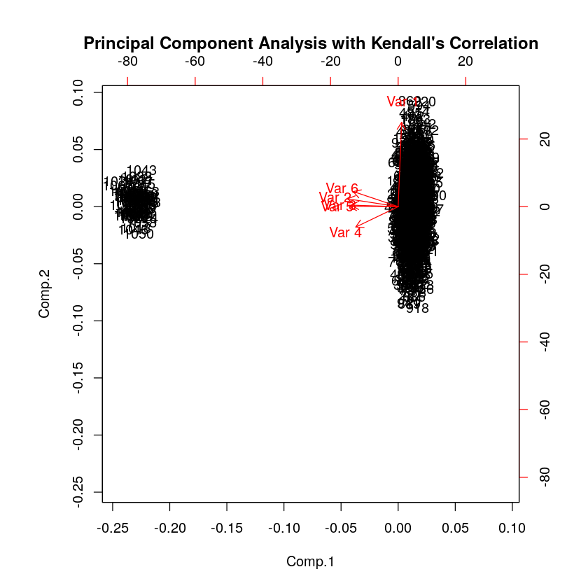
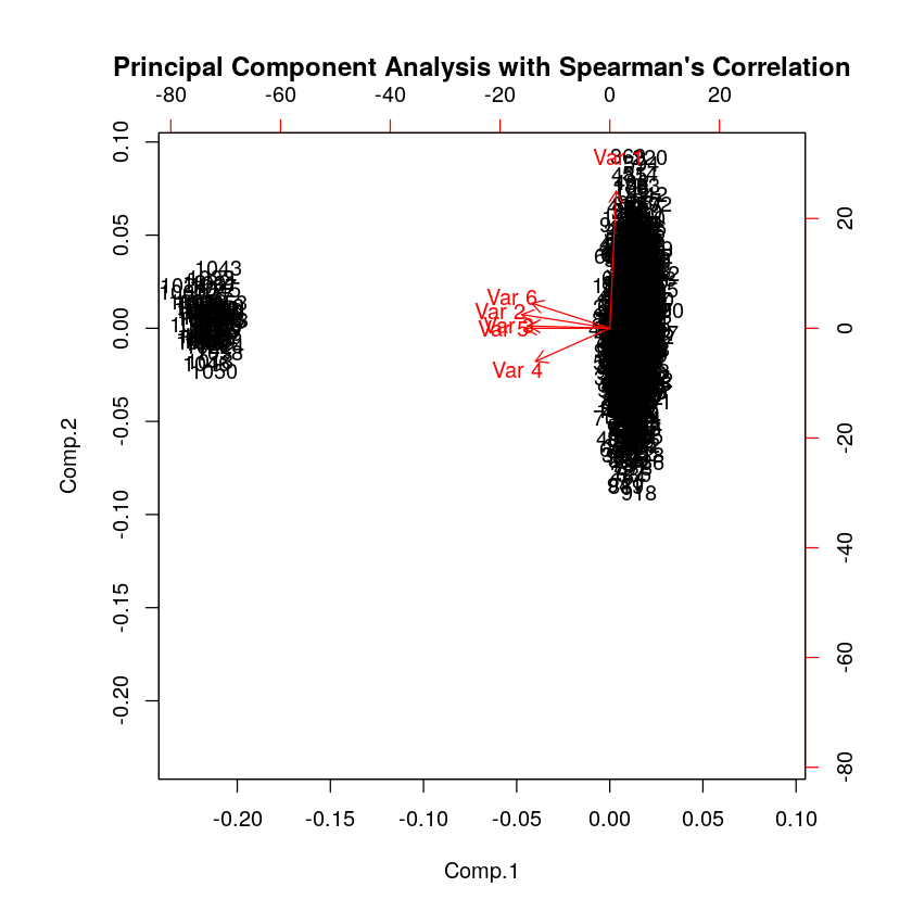
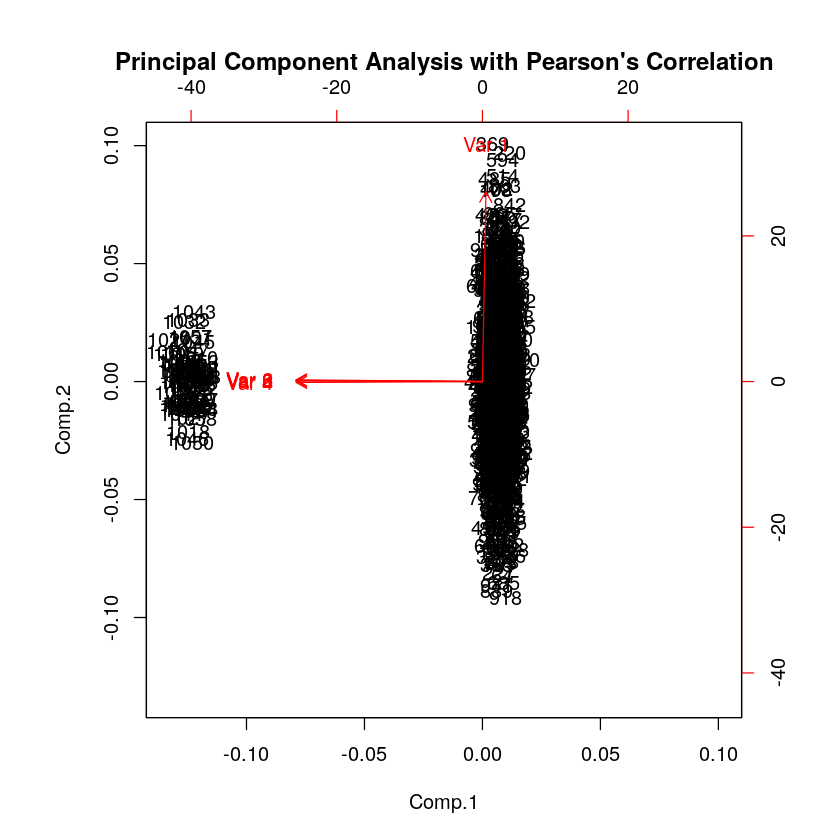
Consider a data set of 6 normal distributed random variables with mean $0,1,\dots,5$ and covariance matrix given by diag $(5,1,1,1,1,1)$ with 1000 observations each contaminated with 60 observations of a normal distribution with mean 20 and variance 5. In Figure 1 are the graphics for the performance of the Principal Component Analysis with the correlation of Pearson (the regular correlation)(1c), the Kendall’s $\tau$ (1a and the Spearman’s correlation (1b)
The difference of performance between the last two no-parametric correlation coefficients between the variables is noticeable, in terms of how much the directions of the principal components respond to the presence of outliers in the data, compared to the regular PCA. It is also true that the estimators tend to go a little to the contaminated data, but still preserve a lot of the structure of the clean data.
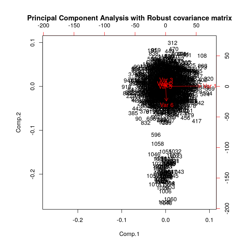
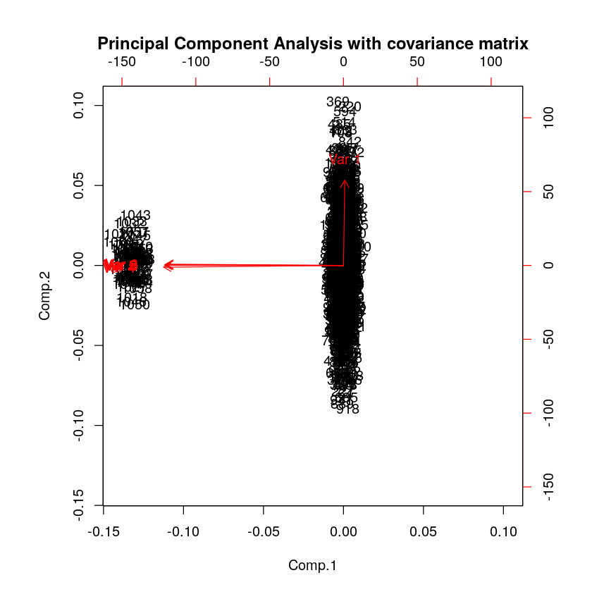
In Figure 2 we can see the performance of the Principal component analysis using the robust estimation of the covariance matrix proposed in the previous section and the usual covariance matrix. Again, the usual is sensitive to outliers, while the robust matrix can perform better in the core of the data, given more precise directions for the principal components.

Refer to caption — (a) PCA using the Kendall’s $\tau$ for correlation matrix

5.2 Projection pursuit approach

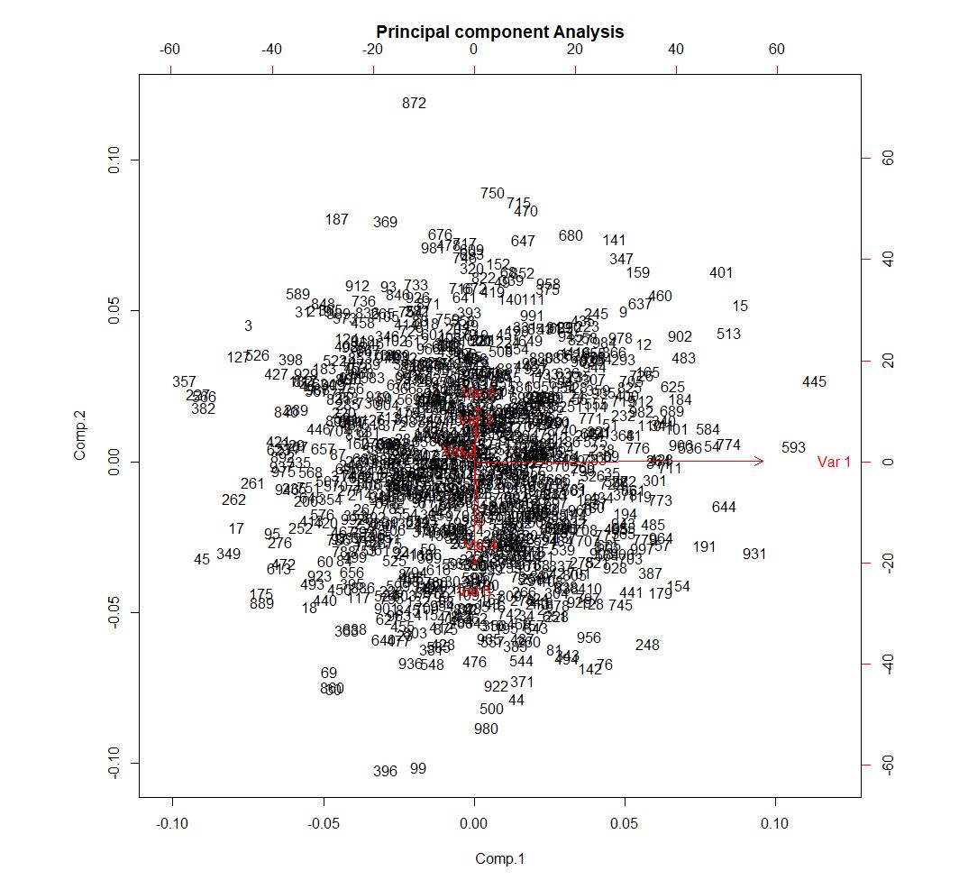
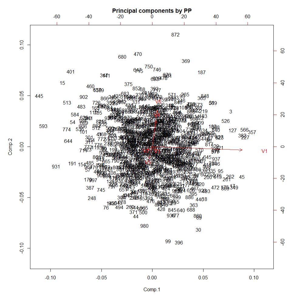
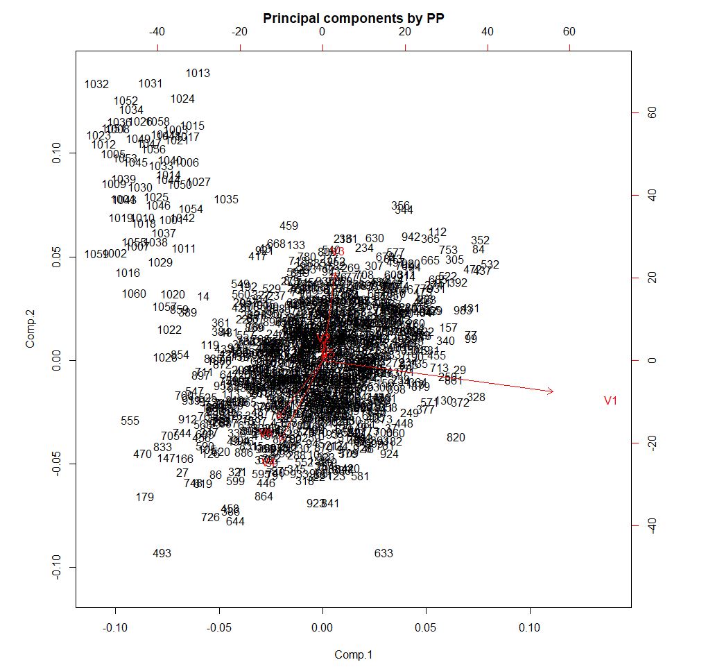
Consider, again, a data set of 6 normal distributed random variables with mean $0,1,\dots,6$ and covariance matrix given by diag $(5,1,1,1,1,1)$ with 1000 observations each. We apply the classical Principal Component Analysis to the data and obtain the results shown in the Figure 3a, and also apply the algorithm for projection pursuit PCA, obtaining the results shown in the Figure 3b. As one can notice, the results are pretty similar.

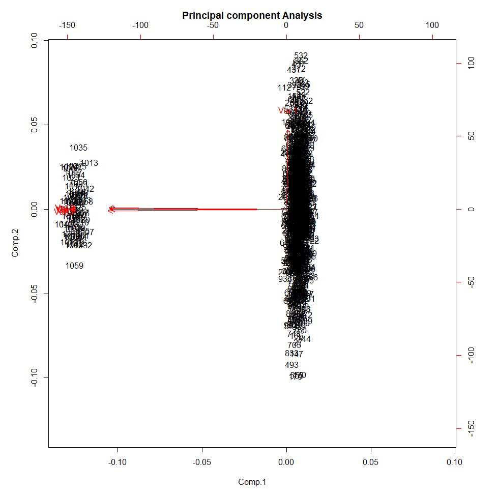
Introducing atypical observations to the data, coming from a normal distribution with mean 20 and variance 1, we analyze the performance of both methods in the Figure 4. Is easy to verify that classical PCA is very sensitive to analysis, and the projection pursuit approach keeps the directions from the core of the data, surpassing the outliers.

6 Conclusions

We presented three different ways to perform PCA that are in some way robust to outliers presence in the data considered. One of them makes use of robust estimators of theprevipus steps for the anlaysis itself, and the other ones make the whole proces more robust to the presence of atypical data.
This is useful for the analysis of real problems, in which data of unknown distribution and possible contaminated values by human or numeric errors or wrong sampling can appear, because it preserves a great part of the original structure of the data and gives points to analyze it from its core, without being drown to the outer layers by atypical values.

References

Campbell, (1980) Campbell, Norm A. 1980. Robust procedures in multivariate analysis I: Robust covariance estimation. Applied statistics, 231–237.
Croux & Ruiz-Gazen, (1996) Croux, Christophe, & Ruiz-Gazen, Anne. 1996. A fast algorithm for robust principal components based on projection pursuit. Pages 211–216 of: Compstat. Springer.
Croux & Ruiz-Gazen, (2005) Croux, Christophe, & Ruiz-Gazen, Anne. 2005. High breakdown estimators for principal components: the projection-pursuit approach revisited. Journal of Multivariate Analysis, 95(1), 206–226.
Croux et al. , (2007) Croux, Christophe, Filzmoser, Peter, & Oliveira, Maria Rosario. 2007. Algorithms for projection–pursuit robust principal component analysis. Chemometrics and Intelligent Laboratory Systems, 87(2), 218–225.
He et al. , (2010) He, Ran, Hu, Baogang, Yuan, XiaoTong, & Zheng, Wei-Shi. 2010. Principal component analysis based on non-parametric maximum entropy. Neurocomputing, 73(10), 1840–1852. = http://www.sciencedirect.com/science/article/pii/S092523121000144X.
Ibazizen & Dauxois, (2003) Ibazizen, Mohamed, & Dauxois, Jacques. 2003. A robust principal component analysis. Statistics, 37(1), 73–83.
Noether, (1981) Noether, Gottfried E. 1981. Why Kendall Tau? Teaching Statistics, 3(2), 41–43.
Rencher, (2003) Rencher, Alvin C. 2003. Methods of multivariate analysis. Vol. 492. John Wiley & Sons.
Zar, (2005) Zar, Jerrold H. 2005. Spearman rank correlation. Encyclopedia of Biostatistics, 7.