Radio pulsar polarization as a coherent sum of orthogonal proper mode waves
Abstract
Radio pulsar polarization exhibits a number of complex phenomena that are classified into the realm of ‘beyond the rotating vector model’ (RVM). It is shown that these effects can be understood in geometrical terms, as a result of coherent and quasi-coherent addition of elliptically polarized natural mode waves. The coherent summation implies that the observed tracks of polarization angle (PA) do not always correspond to the natural propagation mode (NPM) waves. Instead, they are statistical average of coherent sum of the NPM waves, and can be observed at any (and frequency-dependent) distance from the natural modes. Therefore, the observed tracks of PA can wander arbitrarily far from the RVM, and may be non-orthogonal. For equal amplitudes of the NPM waves two pairs of orthogonal polarization modes (OPMs), displaced by , can be observed, depending on the width of lag distribution. Observed pulsar polarization mainly results from two independent effects: the change of mode amplitude ratio and the change of phase lag. In the core region both effects are superposed on each other, which can produce so complex behaviour as observed in the cores of PSR B193316, B123725 and J04374715. Change of the phase lag with frequency is mostly responsible for the observed strong evolution of these features with . The coherent addition of orthogonal natural waves is a useful interpretive tool for the observed radio pulsar polarization.
Keywords:
pulsars: general – pulsars: individual: PSR J04374715 – pulsars: individual: PSR B123725 – pulsars: individual: PSR B191921 – pulsars: individual: PSR B193316 – radiation mechanisms: non-thermal.1 Introduction
Radio pulsars exhibit a wealth of polarization phenomena that have been studied for half a century. However, both the regular polarization properties as well as peculiar effects escape thorough understanding. The regular behaviour includes the appearance of two orthogonal polarization modes (OPMs) and transitions (jumps) between these OPMs at several longitudes in a pulse profile. Peculiar effects are numerous and involve strong deformations of polarization angle (PA) curve, especially at the central (core) profile components (Smith et al. 2013, hereafter SRM13; Mitra et al. 2015, hereafter MAR15) as well as ‘half orthogonal’ PA jumps (Everett & Weisberg 2001; MAR15). The research on the subject includes the analysis of the natural propagation wave modes in magnetised plasma (Melrose 1979; Lyubarskii & Petrova 1999; Rafat et al. 2018), curvature radiation properties (Gangadhara 2010), numerical polarized ray tracing (Wang et al. 2010), coherent (Edwards & Stappers 2004) and noncoherent deconvolution into separate modes (Melrose et al. 2006; McKinnon 2003), instrumental noise effects (McKinnon & Stinebring 2000) as well as interstellar propagation effects (Karastergiou 2009; McKinnon & Stinebring 1998). This is accompanied by a steady increase in the available polarization data of ever increasing quality (eg. recently Rankin et al. 2017; Brinkman et al. 2018).
In this paper I develop the polarization model based on coherent addition of waves in two orthogonal propagation modes (Dyks 2017, hereafter D17). The extended model offers a more general nature of the observed PA tracks and solves several interpretive obstacles that have appeared in D17.
In Sect. 2 I describe observations and modelling hints that inspired this study. These suggest the importance of equal modal amplitude in pulsar signal, so in Sect. 3 I describe a special-case model based on coherent addition of linearly polarized waves of equal amplitude. The model is used to interpret observations in Sect. 4, which is a good opportunity to present the model properties. Since the equal modal amplitudes may be driven by a circularly polarized signal, in Sect. 5 the model based on the circular feeding is extended into a ‘birefringent filter pair’ model which is applied to the issue of why the OPMs are so often observed nearly equal. Section 6 describes the double, ie. convolved or mixed nature of the polarization observed in the core profile region such as demonstrated by the case of PSR J04374715. The equal amplitudes and linear polarization of the natural mode waves cause some interpretive problems (described in Sect. 6.2), therefore, the ellipticity and different amplitudes of the modal waves are taken into account in a more general model described in Sect. 7.1. A glimpse of the properties of the model’s parameter space is given in Sect. 7.2. Interpretive capabilities of the model are presented in Sect. 7.6 where the PA loop of PSR B193316 is modelled at two frequencies.
2 Inspiring observations and modelling hints
2.1 Observations


Fig. 1 presents the polarized profile of PSR B191921 as observed by MAR15. The profile exhibits a sharp PA jump near the maximum flux in the profile. The PA is plotted twice at a separation of which shows that the change of PA at the jump is near perfectly equal to . This may seem not strange given that the jump coincides with deep minimum in the linear polarization fraction and with a sign change of the circular polarization fraction . These are trademark features of the equal modal power, and are frequently observed at the regular OPM jumps. However, after some wiggling on the trailing side of the profile, at the pulse longitude the PA makes another downward transition, quickly followed by a more standard upward OPM jump at .
When moved up by , the displaced central PA segment (between and ) provides roughly rectilinear interpolation between the PA observed outside of the segment. This suggests that the PA stays at the distance through most of the pulse window, and there must be some geometric reason for this. The shift seems to exist despite a clearly nonzero level of both and . Fig. 18 in MAR15 shows that a chaotic multitude of different PA values are observed within the displaced-PA interval of pulse longitude.
As can be seen in Fig. 2, based on Fig. 7 in Everett & Weisberg (2001), PSR B082326 also shows a jump which is coincident with a minimum in . In this case, however, the profile of does not seem to be affected by the phenomenon.
In D17 the half-orthogonal PA jump has been interpreted as a sudden narrowing of a phase delay distribution, with the delay measured between two linearly polarized waves, supposedly representing the waves of natural propagation modes. The small delays imply coherent addition of waves, which ensures the PA jump as soon as the waves have equal amplitudes. However, this rises interesting questions. First, what makes the amplitudes equal, and second – having two pairs of orthogonal PA values off at -- which pair coincides with the PA of the supposedly quasi linear11 1 Hereafter, the terms ‘linear’ or ‘circular’, when referring to signals, waves or modes, should always be understood as ‘linearly polarized’ and ‘circularly polarized’, respectively. natural polarization modes? Below I will confirm the idea of the lag-distribution narrowing, however, the identification of the modes will be shown to depend on whether equal modal amplitudes can be sustained in pulsar signal.
Another type of interesting polarization phenomenon is the exchange of the observed modal power with increasing frequency . This is well illustrated in Figs. 4 and 5 of Young and Rankin (2012) where single pulse PA distributions are shown at two frequencies for PSR B030119 and B113316.22 2 The authors do not comment on this exchange at all. In Fig. 3 I show a cartoon representation of this effect. The PA distribution in each pulsar reveals two enhanced PA tracks that follow a pair of well defined rotating vector model (RVM) curves, with each PA track apparently representing a different OPM. However, the primary (ie. brighter) mode track at 327 MHz becomes the secondary (fainter) track at 1.4 GHz. According to the authors, the data were corrected for the interstellar Faraday rotation, various instrumental effects and dispersion. Moreover, the apparent replacement of the modal power is confirmed by a probably concurrent change in the sign of . The power of the observed OPMs is then partially separated not only in pulse longitude and drift phase (Edwards & Stappers 2003; Rankin & Ramachandran 2003; Edwards 2004), but also in the spectral domain (Noutsos et al. 2015). This may seem to be natural, because the modes are generally expected to have different refraction indices, each with different dependence on , which implies a -dependent phase lag between the modal waves. In the model of D17, however, any changes of the phase lag could not affect the ratio of modal power. This lack of flexibility makes the -related considerations difficult and calls for the model extension.

Another type of insightful polarization effects are the distortions and bifurcations of polarization angle tracks, especially those observed within the central (core) components of pulsars such as PSR B123725 (SRM13), B193316 (Mitra et al. 2016, hereafter MRA16), B185726 (Mitra & Rankin 2008), and B183909 (Hankins & Rankin 2010). All these phenomena reveal clear signatures of their coherent origin: they have maxima of coincident with minima of . The loop-like PA distortion of B193316 was modelled in section 4.4.1 in D17, whereas the PA track bifurcation of B123725 was interpreted in section 4.7 therein. Here those interpretations will be modified and will be made consistent with each other.

An interesting example of the core PA distortion is provided by the millisecond pulsar PSR J04374715 (Navarro et al. 1997, hereafter NMSKB97, Oslowski et al. 2014). As shown in Fig. 4 (after NMSKB97), at 660 MHz the PA curve steeply dives to the vicinity of orthogonal mode, then immediately retreats in another nearly full OPM jump. The retreat is associated with the sign change of and a minimum in (which is not quite vanishing). The first quasi-OPM transition, however, is associated with a high level of . Section 4.4 in D17 describes an effect of symmetric twin minima in which are associated with symmetric profile of . Both these minima have identical look and identical origin. In PSR J04374715, however, the observed minima are dissimilar and have clearly different origin. Moreover, when viewed at different frequencies (NMSKB97) the minima seem to move in longitude at a different rate. They seem to pass across each other which is apparently related to -dependent amplitudes of the negative and positive , and is accompanied by strong changes of PA distortions. Overall, the behaviour of polarization in PSR J04374715 looks as a clear manifestation of two independent processes that overlap in pulse longitude.
Another strange polarization effect can be seen on the trailing side of the core component in J04374715 (Fig. 4, ). The PA there seems to be freely wandering with no obedience to any RVM-like curve. Off-RVM PA values must also be involved in a phenomenon of non-orthogonal PA tracks, that is often observed in many pulsars (eg. B194417 and B201628, both at GHz in Fig. 15 of MAR15). Apparently, any successful pulsar polarization model must be capable of easily detaching from RVM.

2.2 Modelling hints
The PA loop of B193316 has been interpreted in D17 as a sudden rise (and a following drop) of a phase lag between two linearly polarized orthogonal waves, supposedly representing the natural propagation modes. The model is quite successful because it can reproduce all relevant polarization characteristics, such as the nearly bifurcated distortion of PA, the twin minima in , and the single-sign with a maximum at the modal transition. Moreover, with a change of a single parameter (amplitude ratio of modes) the model consistently reproduces the change of these features with frequency . All this occurs because within the loop, the underlying PA track (which gets split into the loop as soon as the lag is increased) is assumed to be displaced by about from the linear natural modes.
However, the data (see Fig. 1 in MRA16) clearly show that the loop opens on a PA track that can be considered as one of the normal OPMs (as evidenced by a regular OPM jump observed just left to the loop). The model thus requires the modal power to be away from where the power is actually observed to be, if the identification of the observed OPMs as coincident with the normal modes is correct. As described in D17, the observed OPMs are sharp spikes of radiative power with the PA coincident with that of the natural propagation modes. As shown in Fig. 5 the observed orthogonal modes (M1 and M2) are produced when the phase lag distribution extends to , since at this value a linearly polarized input signal of any orientation is always decomposed into polarization ellipses aligned with the linearly polarized natural (proper) modes m1 and m2. As emphasized in D17, the observed OPMs (M1 and M2) are not the same as the proper modes m1 and m2, because M1 and M2 may have the same handedness despite being orthogonal to each other (such case is shown in Fig. 5). However, M1 and M2 have the same PA as the proper (normal) waves. Therefore, the linearly-fed observed OPMs M1 and M2 will be called below the ‘coproper’ modes.
Because the above-described difference was hard to justify, the analysis that followed in D17 attempted to interpret the core polarization through changes of mode amplitude ratio with pulse longitude (instead of the phase lag). The amplitude ratio was parametrized by the mixing angle , i.e. the angle at which the emitted signal was separated into two linearly polarized natural mode waves (Fig. 5a). Because of the partial geometrical symmetry of the problem, slow changes of with pulse longitude were essentially able to justify the core polarization behaviour of B123725, at least for the upper branch of its bifurcated PA track.
However, PSR B123725 exhibits two different states of subpulse modulation: the normal state (N) and the core-bright abnormal state (Ab). In the N state the core PA mostly follows the upper branch of the split PA track, whereas the lower branch is brightest in the Ab state (cf. Figs. 1 and 6 of SRM13). Despite the change of the branch, however, the sign of remains the same in both cases. In the -based model of D17 (section 4.7 therein) this was impossible to achieve, because the diverging branches of the bifurcated track were interpreted purely through departure of from a natural mode in two opposite directions, and the predicted sign of is different on both sides of the proper mode. This can be seen in the lag-PA diagram of Fig. 6 which presents selected polarization properties of a wave that is a coherent combination of two orthogonal and linearly polarized waves oscillating at a phase lag . The sign of , as represented by the grey and bright rectangles, is opposite on each side of (which corresponds to one natural mode). Moreover, both the loop of B193316 and the PA bifurcation of B123725 look as phenomena of the same nature, so it is not Ockham-economic to interpret them in different ways (change of phase lag versus change of mixing angle). In the case of the PA loop of B193316, the model based on the only, could reproduce the twin minima, the single-sign , and the PA distortion, but was incapable to produce the loop-shaped bifurcation itself (see Fig. 11 in D17). The bifurcation, instead, required the change of the lag (Figs. 12 and 13 in D17).
Below I further elaborate the models of D17 in order to explain the mysterious misalignment which allows us to interpret both phenomena within a unified scheme.
3 Introductory model
3.1 Coherent addition of linearly polarized waves
Let us start with the model described in D17: before reaching the observer, a radio signal of amplitude is decomposed into two linearly polarized waves with orthogonal polarization:
| (1) |
The waves may be thought to represent the natural propagation modes of a linearly polarizing, birefringent intervening medium. The main (proper) polarization directions of the medium are and . After a phase delay is built up between the waves, they combine (are added) coherently, which produces the detectable radio signal. The amplitudes of the combining waves are equal to
| (2) |
where is the mixing angle that parametrizes the amplitudes’ ratio:
| (3) |
The Stokes parameters for the resulting wave (i.e. calculated after the phase-lagged components have been added coherently in the vector way) are given by:
| (4) | |||||
| (5) | |||||
| (6) | |||||
| (7) |
whereas the linear polarization fraction and the resulting PA are:
| (8) | |||||
| (9) |
To calculate the observed PA, the coherent-origin angle of eq. (9) needs to be added to the external reference value determined by the rotating vector model:
| (10) |
Since we focus on coherent effects, only the value of will be discussed below, but it must be remembered that corresponds to , ie. the RVM PA corresponds to the orientation of the intervening basis vectors ( or ) on the sky.
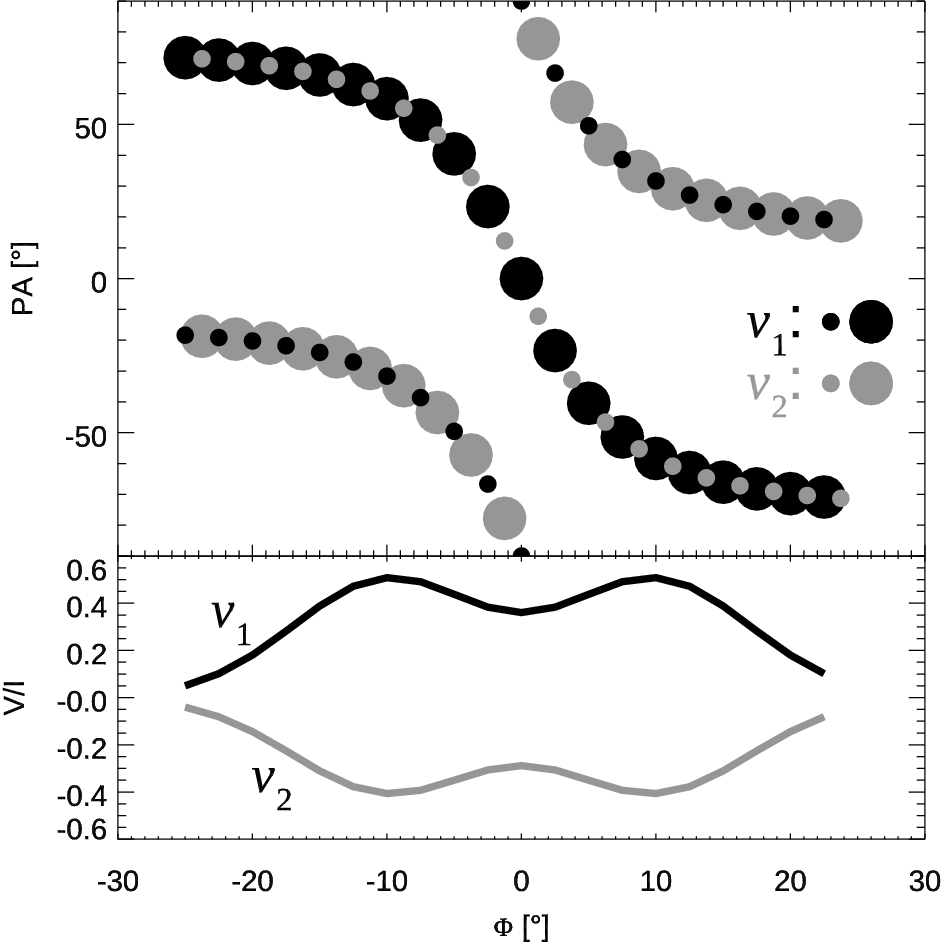
Diverse pairs of in such model give the polarization characteristics presented in Fig. 6. Different curves in the lag-PA diagram (bottom panel of Fig. 6) present calculated for different values of . The value of is fixed along each line, except from the horizontal lines at . In this equal-amplitude case the PA jumps discontinuously by , which corresponds to the transition of the polarization ellipse through the circular stage (see the rows of ellipses in the top panel). The grey rectangles (actually squares) represent the regions with positive . In spite of the impression made by the checkerboard pattern, the sign of can change only at , where is an integer. A change at is impossible, because no lines cross these values of , except at the dark nodes at corners of the grey regions. The nodes appear because for any orientation of the incident wave polarization (hence any amplitude ratio ) produces a polarization ellipse aligned with either or direction of the intervening polarization basis (see D17 for more details).
Because of the noisy nature of pulsar radio emission, in the following numerical calculations the values of and are drawn from statistical distributions and with peak positions and and widths , . The intensity is taken as . The results presented in sections (3)-(6) are produced with the same numerical code which is described in detail in sections and of D17.

3.2 Another pair of orthogonal polarization modes – equal wave amplitudes
Unlike in D17, however, it is assumed in this section that the incident signal can be represented by two circularly polarized waves of opposite handedness.33 3 As discussed below, such circular waves can be produced by a decomposition of an elliptically polarized wave in medium with circularly polarized natural propagation modes. For simplicity of interpretation, in this introductory model the detection of these circular waves (C+ and C- in Fig. 7a and b) is assumed to be non-simultaneous (ie. the signal produced by C+ is not added coherently to the signal produced by C-). Consider the wave electric vector which traces a spiral that projects on the dotted circle C+ in Fig. 7a. In the aforementioned linearly-polarizing birefringent medium, the wave induces the two linearly polarized waves, marked m1 and m2, and described by eq. 1. The original phase delay between the waves is equal to which results directly from their circular feeding. This phase lag is assumed to be increased (or decreased) by different refraction indices of the natural propagation modes (therefore, the wave m1 is shifted to the dashed sinusoid position). Then the modal waves m1 and m2 are coherently added, which produces the elliptically polarized observed signal which is presented by the grey ellipse marked C1. This is one of the observed OPMs (or one observed PA track, if the name OPMs is to be reserved for the linearly fed coproper OPMs of D17). The eccentricity and handedness of the C1 ellipse depends on the value of the lag, however, as long as is between and all the resulting ellipses will have the same PA, precisely at the angle of with respect to the PA of the natural propagation modes.44 4 This makes such circular-fed -off modes statistically frequent, which is a feature analogical to the linear-fed modes of D17. Larger lags produce another orthogonal ellipse, which is marked CA in the figure. This second ellipse is away from C1 and, therefore, may possibly be called the other OPM. However, the CA mode may have the same handendess as C1, so perhaps it should be called a pseudomode.55 5 Though CA may have the opposite handedness too. As explained below, to account for the observed phenomenology, it is necessary to introduce a separate circularly polarized signal of opposite handedness, denoted with C- and in Fig. 7b. This additional wave, in the same way as just described, produces the second observed OPM, marked with the grey ellipse C2. Again, as explained below, the mode may be accompanied by a pseudomode CB, which may have the same or opposite handedness as C2.
Remarkably, the new observed modes C1 and C2 form a pair which is away from the natural modes m1 and m2. They are also mid way between the linear-fed modes described in D17, which have the same PA as m1 and m2. The new circular-fed OPMs66 6 The OPMs may also be called same-amplitude OPMs, especially that the circular feeding may be considered irrelevant to the problem as soon as the equal amplitudes are considered as an ad hoc assumption. See, however, Sect. 5. can be readily handled with the mathematical model described above, because each observed mode results from coherent addition of phase lagged, linearly polarized orthogonal waves (m1 and m2). Specifically, equal amplitudes of the waves imply the mixing angle of (eq. 3) and the circulating feeding of the waves implies the initial phase lag of . These are the positions at which the waves and have to be injected into the lag-PA diagram of Fig. 6. Accordingly, Fig. 8 presents the lag-PA pattern that appears for a single feeding wave (C+) injected at . Each set of panels in the figure may be considered as presentation of signals detected at a fixed pulse longitude in many different pulse periods. The value of was sampled from a narrow Gaussian distribution of width whereas had the width (both distributions are shown near the plot axes). The right panels present the distribution of PA angles at a fixed pulse longitude, i.e. they present a vertical cut through those grey-scale PA histograms that are usually shown for single-pulse data (the black thick solid line is the intensity cumulated at a given PA). The distribution of is shown with thick grey line and is thin solid. Fig. 8a shows the case of a one-sided lag distribution, whereas the bottom panels show the symmetric . Comparison of panels a and b implies that a single circular feed (eg. C+ at ) can produce two orthogonal PA tracks depending on the shape and position of . The difference of refraction indices favours the one-sided , and it is also the case which avoids some depolarization typical of the two-sided . For the moderately wide lag distribution used in Fig. 8, the power stays close to and therefore is high (). is about in the top case, and the same in both PA tracks of the bottom-right panel. However, after Stokes-averaging over the PA distribution, the average (at some longitude ) would be very low, unlike in the top case. The symmetry of distribution is thus important for some conclusions of this paper.
As can be seen in Fig. 8, the lag distribution is extending the grey PA pattern horizontally at and it is these horizontal extensions (which can look as dark horizontal bars – see the next figure) that correspond to the observed OPM ellipses C1 and C2 in Fig. 7. The more these ‘dark modal bars’ are centered at , the higher is the local (in a single PA track) and the smaller is (this can be deduced from top panel of Fig. 6).
The important general implication of this section is that after statistical averaging over , the observed OPMs (or the observed PA tracks) have the PA that is different from the PA of the natural mode waves m1 and m2 (this PA is equal to 0 or , as measured from the axis of Fig. 7). In the specific case considered (equal amplitudes of the natural modes, ), the observed OPMs are located mid way between the natural modes. Thus, the observed PA tracks are not equivalent to the natural mode waves. As shown further below (Sect. 7.5), the PA tracks may in general be displaced by an arbitrary, mode-amplitude-ratio-dependent angle (and a -dependent angle) from the natural modes. In the special case of equal amplitudes (of the natural mode waves m1 and m2) the two observed PA tracks (C1 and C2, or C1 and CA) are separated by from each other, and can easily be misidentified as the natural orthogonal modes, although they are misaligned by from the natural modes m1 and m2.


4 Basic properties of the equal-amplitude OPMs and their application to pulsar problems
For the circular origin of the coherently combined waves m1 and m2, the value of is fixed and must be narrow. Therefore, we are left with only three different processes that can happen to the radiative power on the lag-PA diagram: 1) the lag distribution may move to larger (or smaller) values; 2) the lag distribution may become wider, and 3) the other orthogonal circular-fed OPM can be added as an additional distribution at , i.e. the ratio of amplitudes of and may change.
4.1 Movement of the phase lag distribution
Fig. 9 shows what happens when the phase lag distribution of Fig. 8b moves towards larger values of . In Fig. 9a is centered at which is larger than , hence of the bottom PA track (at ) becomes negative (compare the grey curves in 8b and 9a). The sign of can thus change within the same PA track. In Fig. 9b the PA track makes an OPM transition to the upper value of , however, the circular polarisation stays negative, as in Fig. 9a. Thus, the increase of the lag can cause some OPM transitions, but they do not coincide with the sign change of . They are actually a quarter of lag-change cycle away, so that the OPM jump occurs at a maximum , while the sign change of occurs well within a stable modal PA track, i.e. within flatter parts of a ‘non-transiting’ observed PA track. This is similar to the lag-driven effects in the coproper modes described in D17. The orthogonal modal tracks created by the change of lag (or by widening of ) can thus be called pseudomodes – they do not obey the normal rule of zero at the minimum . A phenomenon of this type (ie. lag-change-based) is observed in several pulsars, eg. in the core PA bifurcations. The lag-driven transfer of power between different OPM tracks also explains the same sign of in different OPM tracks, as observed in single pulses (MAR15). Superficially similar pseudomodal behaviour is also observed in the form of slow OPM transitions at high that occur within the whole pulse window (eg. in PSR B191316, see Fig. 1 in D17, after Everett & Weisberg 2001, also PSR J19002600, Johnston & Kerr 2018). However, these are probably caused by the PA wandering which is discussed further below.

The appearance of the equal-amplitude observed modes at the distance from the natural modes is interesting: it seems to automatically solve the problem of what the primary observed OPM is doing half way between the natural modes at the entry to the PA loop of B193316. It is sufficient to claim that the observed OPMs are away from the natural modes, because their amplitude ratio is close to at this particular frequency. In such case, the PA loop can be explained by a rise and drop of , such as marked with the backward-bent arrow in Fig. 10b (right). The resulting loop is shown in Fig. 13 of D17. Such model reproduces several observed properties, such as the bifurcation of the PA track, twin minima in , and the single-sign (negative) . Moreover, a change of lag within a larger interval, such as shown in Fig. 10b (left) would explain the PA track bifurcation of B123725, along with the sign-changing at the core component.
The lag-induced PA bifurcation is also illustrated with the curved arrows in Fig. 6. It can be seen that for the PA track to split, the radiative power must be close to (in such case the lines of fixed diverge up and down from ). Both the upward- and downward-heading arrows remain all the time within the grey rectangles of positive . Thus for the lag-induced PA bifurcation the sign of stays the same whether the upper or bottom branch of the bifurcation is followed. This would explain why the sign of is the same in both modulation states in B123725: in the bright-core Ab modulation state the lower branch of the bifurcation is followed, but the sign of does not change (in comparison to the N state).
It is thus found that the lag change is the key factor that affects the PA bifurcations observed both in B193316 and B123725. Both these phenomena have the same nature, and can be explained by the same model with slightly different parameters. However, the PA loop of B193316 may also be interpreted in a different (and better) way, which retains the usual coproper OPMs (with the same PA as the natural waves m1 and m2 at 0 and ), but assumes a quick change of towards within the loop. This new interpretation is favoured as discussed later, but such new model also requires the rise and drop of the phase lag within the loop.
The PA bifurcation model that is based purely on the lag-change faces serious problems when the loop of B193316 is interpreted at two frequencies. In Sect. 4.4.1 of D17 (cf. Figs. 13 and 14 therein) I have shown that a change of a single parameter – – from (at GHz) to at GHz well reproduces the new look of the loop at the higher frequency. This can be inferred from Fig. 6: the curved arrow that follows produces the PA amplitude of almost . A similar arrow (not shown) that would follow for the same range of lag, would produce a smaller amplitude of PA, consistent with the data at GHz (see Fig. 1 in MRA16). The problem is that the change of is most naturally associated with the change of phase lag. Even if the mode amplitude ratio (hence ) changes with , it is hard to argue that the lag does not change. For a smaller , the horizontal backward-bending arrow in Fig. 10b (right) would turn back earlier, which would have made the PA amplitude smaller (as observed). However, such earlier backward turn would also cause the twin minima in to approach each other, or even merge into a single minimum at the middle of the loop. This is not observed at GHz: the minima in become very shallow but stay at the same (Fig. 1 in MRA16).
Apparently the lag-change alone cannot explain the loop at both frequencies. It will be shown below that simultaneous change of and with pulse longitude is needed to understand the phenomenon at both frequencies.
4.2 Changes of width of the lag distribution
Considerable widening of the lag distribution wipes out the circular polarization and tends to produce two highly linearly polarized PA tracks of similar or equal amplitude (which gives zero net at a given ). This is because the radiative power is filling in several ‘dark horizontal bars’ at both and in the lag-PA diagram. On the other hand, for moderately strong widening of the results may be similar to those of the shift, because the ‘center of weight’ of the widening moves rightward.

An interesting effect appears when the lag distribution becomes narrow and has a comparable width to the distribution (). Fig. 11 has been calculated for and . As can be seen in the right-hand panels, this makes the PA distribution quasi uniform, and the peaks relocate to coincide with the natural propagation modes m1 and m2 (located at PA of and ). The degree to which the peaks stand out depends on the ratio of and , and increases for narrower . This phenomenon has therefore the key characteristics of the PA jump, namely, the randomization of PA and the appearance of new pair of preferred PA values which are displaced by from the equal-amplitude OPM tracks (observed in the wide- case).
The modelled quasi uniform distribution of PA corresponds to the erratic PA spread observed in the central profile region of PSR B191921, where the average PA curve is displaced by (see Fig. 18 in MAR15). The chaotic (quasi-uniform in the model) distribution of PA becomes visible because the narrow is negligible, so the observed signal directly presents the state with no additional phase lag between the linear components m1 and m2. In this way the circulating motion of the electric field , as presented by the dotted circle C+ in Fig. 7a becomes directly visible (the circulation is recovered as the sum of the m1 and m2 waves with the little-changed original phase delay of ). Surprisingly, then, according to the circular-fed equal-amplitude model, the observed erratic PA spread also has geometric origin: it results from the circulating motion of the incident circularly polarized signal. The observed PA jump thus represents the transition from the lag-spread-stabilized PA (which represents the state of quasi-noncoherent average) to the lag-sensitive chaos of coherent states. In such model, the narrow well defined PA tracks present the observed OPMs (ie. the grey ellipses C1 and C2 that are misaligned by from the natural modes) which are associated with an average of wide -distribution. The longitudes with the erratic PA, on the other hand, present the non-averaged emission in which case the natural propagation modes m1 and m2 get through essentially undelayed. This interpretation, therefore, also associates the observed OPM tracks with the intermodes, just as the aforedescribed PA bifurcation model does.
The PA randomization of Fig. 11 has been obtained for a single OPM signal (say, C1 fed by C+, contributing the distribution at in Fig. 7). In this case the circular polarization can stay larger than zero throughout the jump, as observed in B082326 (Everett & Weisberg 2001) The addition of the second orthogonal mode (C2 or C- in Fig. 7) allows to suppress arbitrarily strongly.
The phenomenon of the jump was interpreted in D17 as the narrowing of the lag distribution, which is maintained here. However, the orthogonal modes that correspond to the wide , and are observed at the profile outskirts in B191921, were interpreted differently, and the peak of the distribution in the narrow lag state was arbitrarily positioned near . In the model discussed in this section the nature of the observed OPMs is different (circular fed C1 and C2) and they automatically tend to stay at the distance from the orthogonal proper waves (m1 and m2).
The widening and displacements of produce the psedomodal behaviour – they are incapable of reproducing the classical mode jumps with coincident minima of and . To obtain such regular behaviour it is necessary to introduce the second circularly polarized component that produces the C2 OPM. This rises the question of why the amplitudes of these circular waves tend to be close to each other, and what causes the amplitude ratio to invert at the regular OPM jumps.


5 Pulsar as a pair of birefringent filters
5.1 Similar amount of pulsar OPMs in the circular-fed model
It has been shown above that some pulsar polarization effects can be described as the linearly birefringent filtration of two circularly polarized waves of similar amplitude but opposite handedness. If added coherently, such circular waves combine into a linearly polarized wave, or an elliptically polarized wave with large eccentricity of its polarization ellipse (see Figs. 12 and 13). This suggests that both these circularly polarized waves (C+ and C-) are generated by a single emitted signal with a narrow polarization ellipse. Such original signal may be split into two circularly-orthogonal waves in medium with circularly polarized natural propagation modes. If the original (i.e. emitted) signal is completely linearly polarized, as in the middle case in Fig. 13, then it produces identical amplitudes of both these circular waves (C+ and C-).
In D17 the circular wave stage of the model was absent. Along with the change of pulse longitude , the electric vector of the emitted linearly polarized signal was slowly rotating with respect to the intervening polarization basis ). The reason was the change of angle between the low- and high-altitude direction of charge trajectories (section 4.5 therein). Whenever the vector was passing through the angle, ie. mid way between and , the mode amplitude ratio was inverted. This was causing the OPM jumps, albeit of the pseudmodal nature (with peaking at the minimum ).
In the present circular-fed model such effect is not possible, because the rotation of the initial linearly polarized (or slightly elliptical) signal does not affect the amplitudes of the circular waves C+ and C-. The rotation just changes the phases of the waves, as shown in Fig. 12 (it is the Faraday rotation effect). Whatever the absolute oscillation phase of the circular waves, they always feed the same, orthogonal and linearly polarized waves m1 and m2. However, the ellipticity and handedness of the initial signal do affect the amplitudes of C+ and C-. As illustrated in Fig. 13, the relative amount of the circular waves is inverted whenever the handedness is changed, and the amplitude ratio is determined by the eccentricity of the initial signal.
Therefore, in the model with the filtration of the initial signal by the circularly-birefringent medium the regular OPM jumps (with the coincident minima of and ) are caused by the change of handedness of the emitted signal. It is the handedness of the emitted radiation which determines which circle in Fig. 7 is larger, and which distribution – whether the one at or the one at – is stronger, i.e. higher.
5.2 The regular OPM jump in the center of radio pulsar profiles
There is a way to test the hypothesis that the regular modal jumps are caused by the handedness change. It is well known that the regular inversion of the mode amplitude ratio is often observed in the central parts of pulsar profiles. The millisecond pulsar PSR J04374715 provides an example of this effect, as evidenced by the sign change of and OPM jump at the normally behaving minimum (see Fig. 4). Such sign-changing, sinusoid-like profile of has long been associated with a sightline traverse through a fan beam of curvature radiation, the latter being emitted by a bent stream of charges (e.g. Michel 1991, pp. 355 - 359). The ensuing pulse of curvature radiation, at least in vacuum theory, has precisely the sinusoid-like, handedness-changing profile of . As a consequence of the geometry shown in Figs. 13 and 7, there should be a regular OPM jump produced by the change of handedness, and it is indeed often observed at zero in such core components of supposedly curvature-radiation-related origin.77 7 The orthogonal elliptically polarized modes have by definition the opposite handedness, so it may seem to be a trivial vicious circle argument that a change of sign confirms a modal jump. However, it is not, because without the final linearly birefringent filtering, the circular waves of Fig. 13 would combine back to the original ellipse or would be observed as separate circularly polarized signals. So it is the pair of filters which produces the regular OPM jumps.
Thus, pulsar magnetosphere consisting of two filters that are made of circularly and linearly birefringent materials provides a quite successful polarization model: it is capable of explaining both the above-described non-RVM peculiarities and the standard polarization properties such as comparable modal power and the regular OPM jumps. However, such model is complex and difficult to justify physically. A possible physical scenario would include a low altitude emission of the nearly linear signal, followed by the circular decomposition in weak magnetic field at large altitudes. The final stage of the linear filtering could possibly be considered as equivalent to the effects that occur at the polarization limiting radius. Because of this complexity, in what follows the relative amplitude of the opposite- modes is considered as a free parameter.
6 Twofold nature of pulsar polarization


It was shown above that aside from the RVM effect, the polarization of pulsar radio signal can change because of two independent reasons: 1) as a result of change of the lag distribution and 2) as a result of change of the modal amplitude ratio (expressed by the ratio in the circular-fed model). The first factor likely depends on the local properties of the intervening matter: a temporary increase of refraction index may appear when the line of sight is traversing through some extra amount of matter, e.g. a plasma stream. The second factor is likely governed by the radio emission process (and is determined by the ellipticity and handedness of the emitted radiation in the specific case of the filter pair model). The two mechanisms – the lag-driven and amplitude-driven changes of polarization – have markedly different properties. The lag-driven effect produces the anticorellated variations of and with pulse longitude (and OPM jumps at maximum ). The amplitude-driven effects generate the regular modal behaviour with the usual OPM jumps.
These generic properties are illustrated in Fig. 14 which presents a regular OPM transition on the left () and the lag-driven bifurcation of the PA track on the right () as a function of pulse longitude. The regular OPM coincides with the mode amplitude ratio of . The relative power of both modes, hereafter denoted , can be expressed as the integrated power (or just height, in case of identical width) of the distribution at and . The increasing value of is shown in the top panel (dotted), along with a temporary increase of (solid Gaussian).88 8 Here ‘temporary’ means ‘constrained to a narrow interval of pulse longitude’. Several polarization effects observed in radio pulsars result from either process, or from a mixture of both. As described in section 2.1, both these non-RVM effects appear to shape the observed polarization especially in the central parts of pulsar profile.
Both these effects may depend on frequency. The influence of the lag may depend on because the lag depends on the refraction index, which is likely -dependent. As for the amplitude-related effects, they need to be -dependent to explain the modal power exchange observed in the D-type pulsars by Young and Rankin (2012). This exchange of power seems to coincide with the -sign change, although the radio spectral coverage is far from continuous.99 9 In the case of B030119, for example, between the 327 MHz and GHz Arecibo profiles of Young & Rankin I have only found the GHz profile in MRA15. The modal exchange takes place near GHz since has both signs in different parts of the average profile at this . The -dependent amplitude ratio is also responsible for another type of PA distortions (slow PA wandering) that is discussed further below.
6.1 The origin of dissimilar minima in PSR J04374715
While interpreting polarization in the central (or other) parts of any profile it is important to allow for the possibility that both the effects of lag and amplitude ratio may be overlapping there to produce a net profile of , and a net PA. An obvious example of such overlap is the center of the profile of J04374715.
Fig. 15 presents model result for the case when the temporary rise of lag (solid line in top panel) roughly coincides in with the amplitude ratio reversal (dotted curve in top panel). The parameters have been changed a bit in comparison to Fig. 14, eg. the rate of change was increased, however, the main difference is that the longitude of equal mode power () and the peak of profile were displaced to roughly the same . This combination of lag and amplitude effects reproduces the major features of the central profile portion in J04374715 at 660 MHz (Fig. 4, after NMSKB97). A double minimum of appears at (denoted FT in Fig. 15). The right minimum in this pair coincides with the change of sign, whereas the left one coincides with high . The value of in the regular right minimum does not quite reach zero, as in the observation. Within the longitude interval flanked by the minima, the PA is visiting the orthogonal PA track, but quickly returns back to the value.1010 10 Since the model is perfectly aligned with , one is free to choose whether the PA jump direction is up or down. The deep minimum at does not follow the observations, but this is only because no efforts have been made to adjust parameters in this longitude interval. Another difference is that the modelled OPM follows the full traverse. This is caused by the perfect alignment of the with (this constraint will be relieved below).
The complex polarization of core emission can thus be understood as a combination of the lag-driven and amplitude-ratio-driven polarization effects. The core emission of normal pulsars (eg. B123725, B193316) also exhibits polarization profiles that are neither symmetric nor antisymmetric. Apparently, the overlap of lag and amplitude effects also occurs in these objects and is partially destroying the anti/symmetry of and which appears when the lag and amplitude phenomena are viewed separately.
6.2 Towards a general model
Let us summarize the results obtained so far. A model based on coherent and quasi-coherent addition of linearly polarized waves of roughly equal amplitude is capable of qualitatively reproducing polarized profiles (ie. all three components: , and PA) of the following phenomena: 1) the bifurcations of PA track in pulsars with complicated core emission (ie. B193316 and B123725, including two modulation states of the latter) and 2) the mixed core behaviour of J04374715. When extended to encompass the origin of the feeding circular waves, the model can possibly justify the regular OPM jumps and the similar amount of modes.
On the other hand, the purely linear birefringent filtering may seem unphysical, and the model faces two problems that contain indications about how to change it. First, the pseudomodal OPM transitions tend to traverse regions of very low . As can be seen in Fig. 6, for increasing from zero at the radiative power approaches the fully circularly polarized point at then jumps down to while staying all the time fully circularly polarized. This is consistent with the low observed at the core PA bifurcations in PSR B193316 and B123725, however, a capability to flexibly adjust the modelled is needed: in the D17’s -based model of B191316 it was difficult to avoid the strong decrease of at the OPM transitions (cf. Figs. 1b and 7b in D17). Second, with the circular feeding of the linear proper waves (m1 and m2), the distribution is absolutely tied to . Actually, even the spread of around these values (parametrized by ) is hard to explain.1111 11 The displacement from could be obtained for elliptically polarized feeding waves.
The circularly polarized waves (C+ and C-) that feed m1 and m2 are then too restrictive for the model and, at least when the ‘filter pair’ concept is dismissed, they indeed do little more than set the equal amplitude ratio of m1 and m2. Therefore, in the following I will use the lone pair of standard, ellipitically polarized, orthogonal natural mode waves (EPONM waves). Obviously, the coherent addition of such waves must produce all the successful results of previous sections, because the linearly polarized equal amplitude waves are just a special case of EPONM waves. However, the arbitrary amplitude ratio and the nonzero ellipticity provide important enlargement of the model capabilities.
A general model of pulsar polarization thus includes the eccentricity of the polarization ellipse for modal waves (m1 and m2). The eccentricity parameter may need to be sampled from statistical distribution of some width. Even with the same eccentricity for both modal waves, this means two new parameters. Along with the other four (the mixing angle for the amplitude ratio and the phase lag, plus the widths of their distributions), this makes up for six parameters. Such parameter space deserves a separate study, therefore, in what follows I describe my calculation method and only present a glimpse of the parameter space – just to address the above-described problems.
7 General model
7.1 Coherent addition of elliptically-polarized orthogonal waves


The model is conceptually simple: observed pulsar polarization results from coherent and quasi-coherent addition of phase-lagged waves in two elliptically polarized natural propagation modes. They are numbered and and are presented in Fig. 16 by the ellipses m1 and m2. These ellipses are traced by the corresponding electric field waves and . The ellipses m1 and m2 should not be mistaken for the observed PA tracks, because the latter result from coherent addition of m1 and m2 and may be easily displaced from the natural modes by an arbitrary angle. For example, if equal amplitudes of m1 and m2 are preferred, then the observed polarization ellipses (similar to the grey ellipses of Fig. 6) appear at the PA of when m1 and m2 are coherently added. The elliptical natural mode waves m1 and m2 can be written as:
| (11) | |||||
| (12) |
| (13) | |||||
| (14) |
where is the phase delay and represents the ratio of the minor to major axis of the polarization ellipse. As usual represents the ratio of the modal waves’ amplitudes, ie. , where and . These waves coherently combine into the observed signal that in general is elliptically polarized:
| (15) | |||||
| (16) |
The polarization ellipse for the observed signal is calculated by numerically increasing in the range between 0 and . The minor half axis and the major half axis of the observed ellipse are then identified numerically, along with the sense of the electric vector circulation (handedness). The PA is determined by the normalized components of the major axis:
| (17) |
whereas the ellipse axes length ratio gives the observed eccentricity angle:
| (18) |
which is different than the initial of the proper modal waves. The normalized Stokes parameters are calculated from:
| (19) | |||||
| (20) | |||||
| (21) |
and the linear polarization fraction is calculated as .
7.2 Lag-PA diagrams for elliptical modes
The lag-PA diagram of Fig. 17 (left panel) presents the pattern of PA calculated for fixed values of eccentricity increasing uniformly from 0 to in step of . The amplitudes of the combined modes are everywhere the same (). The corresponding is shown in Fig. 18, with increasing in darker regions. The sign of is changed several times in the same points of this diagram and, therefore, is not shown. However, is as before anticorellated with , so dark regions in Fig. 18 present low .
The pattern presents new nodes, ie. regions where there is high probablity to observe the radiative flux. The nodes are at and . They appear for two reasons. The first is that for any eccentricity, at the electric vectors of the equal-amplitude modal waves always combine at the PA that is away from the PA of the proper modes (m1 and m2 have the PA of and ). The second reason is that for the purely linear polarization (infinite eccentricity) of equal-amplitude waves the resulting PA is equal to regardless of . This produces the discontinuous PA jumps between the fixed PA values at and . For high eccentricity (nearly linear modal waves m1 and m2), and always for equal amplitude, the PA tends to linger close to , which increases the probability of the nearly intermodal PA. This is illustrated in Fig. 28 of the appendix.
The model described earlier in this paper (with the equal-amplitude linearly polarized orthogonal waves, LPOW) was confined only to the horizontal PA segments centered at the new nodes (and some nearby regions because was allowed to have finite width). The lag-PA space of the LPOW model is just a subpart of the new lag-PA diagram and this is because diverse ellipticities are added in Fig. 17. The patterns of and , within the overlapping part of the parameter space, are identical to the one of the LPOW model. For example, the value of in Fig. 18 increases towards and decreases at the discontinous lag-change-driven OPM jumps. The new nodes coincide with the ‘dark modal bars’ of the LPOW model. This implies that all data interpretations provided before are also possible in the new elliptical model. In other words, the added diversity of eccentricities does not corrupt the previous results.
When the PA values of the left panel are collected in bins on the vertical axis, the histogram shown on the right is produced. The enhancements of the observed OPMs remain at the intermodal positions (half way between the PA of the natural modes). Naturally, for () the intermodal nature of OPMs persists in the presence of diverse ellipticity.
A new feature of the lag-PA diagram are diagonal straight lines which connect the nodes. These correspond to the sum of two circular waves () at increasing lag. The result is a uniformly rotating linearly polarized signal, hence the linear change of PA (the diagonals thus represent the Faraday rotation effect). A similar case is shown in Fig. 12 and Fig. 29 in the appendix. The linear polarization is full along the diagonals (, ).
If the radiation at a given pulse longitude contains a mixture of eccentriticies, then the lag-driven OPM transition occurs both along the S-shaped (or discontinuous) paths in the lag-PA diagram and along the straight diagonals. As shown in Fig. 18, in the middle of the OPM jump the combining signals of high eccentricity (ie. the almost linearly polarized modal waves which follow the S-shaped path) contribute circularly polarized power (note the bright stripe of the high at the position indicated by the arrow) whereas the low-eccentricity signals (circularly polarized modal waves that follow the diagonals) contribute linearly polarized power (the diagonals are black everywhere, ie. they have , see Fig. 29, compare Fig. 28). The lag-driven OPM transition for a signal of mixed ellipticity, can thus be percieved as the passage from, say, the top horizontal row in Figs. 29 and 28, to the fourth row in these figures (along with all unshown cases of intermediate ellipticity). As shown in Fig. 18 with the arrow, the inclusion of wider ellipses increases at the lag-driven OPM jump. The inclusion of eccentricity can thus increase the very low at some lag-driven OPM transitions.


7.3 Entanglement of the lag-driven and amplitude-ratio-driven effects
The amplitude ratio of observed OPMs seems to change with pulse longitude and with the frequency . The lag change should be considered as the primary effect which governs different look of PA tracks at different . The change of mode ratio (or ) is naturally responsible for changes of polarization with (as proved by the regular OPM jumps). However, several observations at different suggest that may also be -dependent. Moreover, if some observed OPMs have the intermodal nature, as illustrated in Fig. 7, then it is the change of lag itself, which causes the ratio of observed OPMs to change. This has been presented in Fig. 9, where the change of lag causes the radiative power to leak from one orthogonal PA track to another. It should be possible to recognize if the observed change of OPM amount has the lag-driven origin, because the lag-driven effects exhibit the pseudomodal behaviour (anticorellation of and ). This complexity needs to be kept in mind when the non-equal mode amplitudes are considered.
7.4 Beyond the equal amplitudes
To move away from , the amplitude ratio of the natural mode waves (m1 and m2) must be changed to a less trivial value than .1212 12 To detach from in the circular-fed equal-amplitude model, it is necessary to consider simultaneous detection (and coherent combination) of the modes C1 and C2. The change of causes the entire lag-PA pattern to evolve. Fig. 19 shows the case of (amplitude ratio of ) whereas Fig. 20 is for (ratio ). As can be seen in Fig. 19, with the change of mode amount ratio the PA paths move away from . Moreover, with the increase of lag many paths cover smaller range of PA than in the equal amplitude case.
It should be noted that the addition of EPONM waves itself does not imply any preference for the same or similar amount of modes. The intermodal observed OPMs (located at , see the histogram in Fig. 17) are just the consequence of the equal amplitude assumption. When the entire parameter space is sampled uniformly in , and , the coproper modes of D17 (with the same PA as the natural modes, see Fig. 5) become statistically most probable and stand out in the histogram (see Fig. 21).
In the case of the linear-fed coproper modes (Fig. 5), the equal amplitudes of observed OPMs are produced when the incident linear signal is traversing through the intermodal separatrix IM (at a wide that extends to ). This seems to be a quite simple and natural way to change the PA by , but the sign of does not change along with the PA jump. In the birefringent filter pair model, the equal/similar amplitudes of both opposite- modes are produced by decomposition of the initial quasi-linearly polarized signal in the circularly polarizing medium of the first filter. Apparently, some mechanism akin to such process is required to explain the nearly equal amount of the modes m1 and m2 which are shown in Fig. 16. In any case, if there is any reason for which the natural mode amplitudes tend to be similar, then the histogram of Fig. 17 tells us that the observed OPMs are actually away from the natural propagation modes (as illustrated in Figs. 7 and 28). The dotted circles in Fig. 16 present how the similar amplitudes of modes can be produced if they are fed by the circularly-polarized waves of common origin (ie. produced by decomposition of an almost linearly polarized signal into the C+ and C- waves of nearly equal amplitude).
Finally, however, it must be admitted that amounts of the opposite- modes are equally often observed to be strongly nonequal. This option opens the possibility to understand the off-RVM wandering of PA tracks.
7.5 Mode-intermode PA transitions and the origin of the off-RVM wandering of PA

7.5.1 Non-orthogonal PA tracks


The primary mode exchange phenomenon, illustrated in figures of Young & Rankin (2012) and other observations clearly show that the mode amount ratio changes with frequency. The ratio (or ) also changes with pulse longitude as proved by the regular OPM jumps and ubiquitous changes of with .
The coherent addition of proper modal waves (m1 and m2) implies that the observed PA should be at (with respect to the proper wave PA) whenever the lag distribution is wide and the modes’ amplitudes are equal.1313 13 For a narrow the observed PA becomes determined by an accidental value of or . A wider allows for the statistically average value to stand out in a stable way. Note that such statistical average of signals with different reproduces the PA value that would be expected for a coherent sum of linearly polarized modal waves at zero lag, ie.:
| (22) |
This equation is valid for other amplitude ratio values, however, for the full uniform distribution of the PA maxima appear as two pairs, visible in the right panels of Figs. 19 and 20, ie. they appear at , and . For a narrower distribution of eccentricities only some of these four peaks remain in the signal. Fig. 22 is calculated for uniform in the range and (hence this case is a subpart of Fig. 19). This gives two PA tracks at , ie. separated by . The phenomenon of non-orthogonal PA tracks is often observed in radio pulsar data. For example, in PSR B194417 and PSR B201628 (Fig. 15 in MAR15) the PA tracks are neither orthogonal nor parallel, which requires the nonequal modal amplitude to change with .
7.5.2 Off-RVM PA wandering
For increasingly non-equal amount of modes, will diverge from and, in the limit of one mode absent, the observed PA must become equal to or , ie. it must start to coincide with one of the natural modes. Therefore, the model predicts that whenever the mode ratio is changing (along with changing or ) between and , the observed PA should exhibit transitions between the observed intermodal PA track (at ) and the proper mode at . In a general case, the PA can wander between some initial and a final , with the values determined by their corresponding mode amplitude ratios, as given by eq. (22).
This type of phenomenon likely occurs on the right side of the 660 MHz profile in J04374715 (Fig. 4). The -dependent modal ratio may also affect the strongly -dependent look of polarization within the core component of this pulsar. However, figures 17-22 clearly show that changes of lag with can affect the observed polarization at least equally strongly, and in fact they do, as is shown in the following section.
7.6 Frequency dependent lag and the loop of B193316
The OPMs observed to the left of the PA loop in PSR B193316 are stable at different frequencies: they look as the same pair of orthogonal patches at both and GHz (see Fig. 1 in MRA16). This holds despite the ratio of observed OPMs quickly changes with pulse longitude at both frequencies. The steady orthogonal location of the modes can be ensured both in the linear-fed model of Fig. 5 and in the circular-fed model of Fig. 7. In the case of the coproper modes of D17, the lag distribution must be wide so that the nodes at PA of and are enhanced. For a narrow distribution the proper modal waves m1 and m2 would coherently combine to an arbitrary PA, as given by eq. (22). Alternatively, the proper modal waves would have to be detected non-simultaneously (to avoid coherent addition) to hold the steady PA at and .
The observed minima in of B193316 (Fig. 1 in MRA16) reveal that the mode amount ratio is being inverted every or so in the profile, so it is natural to assume that temporarily becomes close to unity ( or ) within the loop (where ‘temporarily’ again means ‘within the narrow interval of ’). Therefore, it is assumed in the following that slightly crosses the value of within the PA loop. For simplicity, the eccentricity is set to infinity (linear waves, ) so that the model considered is that of Fig. 5 (which is a special case of the general model shown in Fig. 16). Moreover, since changes of appear indispensable to obtain the bifurcation effect, it is assumed that both and change within the loop.
Fig. 23 presents polarization characteristics calculated for the Gaussian change of and , as shown in panel a with the dotted and dashed line, respectively. Both Gaussians have the pulse longitude width . The values of and are fixed across the pulse window. Outside the loop the modelled PA track follows the proper mode at , because the assumed profile for the peak of the mixing angle distribution is: . When diverges from so much that the intermode is crossed (dotted horizontal at ) the PA loop is opened on the coproper OPM track.1414 14 It is therefore not necessary for the OPMs left to the loop to be intermodal. The loop is not identical to the observed one, but several observed features are reproduced: there are upward-pointing ‘horns’ of PA at the top of the loop, little power inside the loop, and the bottom of the loop extends into the downward-pointing tongue of radiative power that reaches all the way to the top of the loop (after the PA axis is wrapped up with the period). The twin minima in and the single-sign are also well reproduced.
The simultaneous changes of seem to be indispensable in this model. The change of alone does not produce the bifurcation, and the result in such case resembles that of Fig. 11 in D17.
The profile of peak value in the lag distribution was , ie. the amplitude of the lag change is equal to in Fig. 23. When the lag-change amplitude is decreased to , the result of Fig. 24 is obtained. One can see that the loop disappears and is transformed into the U-shaped PA distortion, much like the one observed in the data at GHz (Fig. 1 in MRA16). Moreover, the twin minima in become shallower, but do not merge, again as observed for B193316. The value of increases, while decreases, in agreement with data at both GHz and GHz.
The decrease of lag amplitude is thus the only thing which is needed to understand the evolution of the PA loop with frequency. It is possible to obtain the right behaviour with the decrease of lag only, which is naturally expected at the increased .
The phase lag may be a strong function of and it is possible that becomes negligible at GHz. If so, then the observed PA track of the U-shaped distortion directly reveals the profile of , which is indeed observed to be about away from the OPMs that are observed outside the loop (the dotted curve in Fig. 24a is reproduced in the PA curve of Fig. 24b, to be compared with the GHz data in Fig. 1 of MRA16).
The result of this section again shows that the core polarization of pulsars is a combination of amplitude-driven and lag-driven effects, and the look of PA curves and other polarization characteristics change with frequency, because of the frequency-dependent phase lag. When the Gaussian profiles of and are misaligned, the resulting profiles of and become asymmetric, which is observed at both frequencies. It should be possible to construct a similar multifrequency model for the complex behaviour of core polarization in J04374715 at different frequencies.
It must be noted that several effects of the lag change can also be produced through the narrowing of distribution. For example, a result similar to that of Fig. 23 can be obtained for a fixed (-independent) when is changing within the loop. Reasonably looking loops were in particular obtained for a one-sided with following the profile of . In such case the exact shape of the resulting loop depends on the value.
7.7 Lag-driven inversions of PA distortions
Polarization characteristics that result from coherent mode addition sometimes are very sensitive to the parameters used. The results illustrated in the previous section were calculated for symmetric (two-sided) lag distribution . Fig. 25 presents a different result for a one-sided . The amplitudes of the and profiles are and , respectively, and now increases within the PA distortion (see the dotted line in panel a).
A change of only the lag amplitude to leads to the result of Fig. 26. The PA distortion is now protruding upwards, whereas the other polarization characteristics (such as and do not change much). This phenomenon resembles the PA bifurcation of B123725 in the N and Ab modulation states (SRM13). With the change of modulation state, the observed PA follows different branch of the PA bifurcation while the sign of does not change. It appears possible then, that the exchange of the followed PA branch is caused only by the change of the lag value in different modulation states.


Obviously, the phenomenon of the modulation-state-dependent polarization, and other complex polarization phenomena in pulsars require more detailed study. The parameter space for the coherent addition of non-equal elliptical modes offers a large number of possible polarization profiles. Fig. 27 presents the PA as a function of lag, calculated for a sparse grid of parameters: , , and . Different lines of correspond to different pairs of . A numerical code for pulsar polarization needs to probe even larger parameter space, with the added widths of statistical distributions of , , and . To make things more complex, it may be necessary to introduce a few additional parameters that describe how these six basic parameters depend on pulse longitude . More complete analysis of the phenomena visible in Fig. 27, along with detailed numerical fitting of pulsar data, is deferred to further study.

8 Conclusions
It has been shown that complex non-RVM polarization effects in radio pulsars can be understood in geometrical terms, as the result of coherent and quasi-coherent addition of elliptically polarized orthogonal proper-mode waves. The phenomenon of coherent mode addition is described by three (or six) parameters: the phase lag, the amplitude ratio (mixing angle), and the eccentricity of polarization ellipse (plus the widths of their distributions). The model implies that the observed radio polarization is driven by at least two independent effects: the changes of mode amplitude ratio, which, in particular, are responsible for the regular OPM behaviour (with zero at OPM transitions) and the changes of the phase lag which have opposite characteristics. Both these factors influence the observed polarization within the same pulse intervals, which is evident in the core region of profiles. Such model explains several complicated and dissimilar phenomena, such as: distortions, bifurcations and loops of the PA observed in the central part of profiles, twin minima in associated with these distortions, maxima of at OPM jumps, -off PA tracks, chaotic spread of PA values within the -displaced emission, and dissimilar minima of mixed origin, such as those observed in J04374715. Moreover, the model is capable to interpret the changing look of these phenomena with frequency and possibly with modulation state.
The observed OPM tracks have often been directly associated with the natural propagation mode waves. It has been shown here that the observed OPMs do not necessarily correspond to the natural waves. Instead, the observed OPMs are a statistical average of coherent sum of the natural waves (with diverse phase lags). Therefore, the PA of observed polarization tracks can be completely different from the PA of the natural waves. The observed PA tracks may be non-orthogonal and they may wander away from the RVM PA. The coherent addition model implies that the PA is distorted by the -dependent location and width of the lag distribution, and by the -dependent ratio of modal amplitude, as expressed by eq. (22).
In the noncoherent model the observed PA can only jump by when one mode becomes stronger than another. In the coherent mode addition model, the noncoherent condition is obtained by coherent summation of numerous natural mode waves at diverse phase lags. This typically causes the coproper modes M1 and M2 to stand out in the data. Preference of equal modal amplitudes, however, makes the intermodes C1 and C2 most pronounced.
Identical amplitudes of the natural propagation mode waves (m1 and m2) are automatically produced when the waves are fed by a circularly polarized signal. The coherent addition model then implies that two pairs of observed OPM tracks may in general appear in pulsar profiles, and the pairs are separated by . Just like the linear-fed coproper modes, the intermodal OPMs are pronouced when the phase lag distribution is wide, which introduces many polarization ellipses that all share the same PA of (or , see Fig. 7).
In the case of the linear-fed coproper modes, the psedomodal OPM jumps are produced when is passing through the intermodal value of . is maximum at such OPM transitions. In the case of the circular-fed equal-amplitude OPMs, the regular OPM jumps take place when the handedness of the feeding wave is changed. In the case of the general model with the elliptical proper modes, the regular OPM jumps occur in the usual way (when one mode becomes stronger than another, for whatever reason).
When the mode amplitude ratio slowly deviates from , the observed PA makes a non-orthogonal passage between the intermodal PA value and the natural mode PA, eg. between and . Such change of PA does not have to be precisely equal to given the possible simultaneous change of PA caused by the RVM effect. Examples of such slow wandering of PA between the OPM values can often be found in pulsar data, eg. on the trailing side of profile in J04374715, Fig. 4.
The presented model solves several problems that appeared in the analysis of D17. The complex polarization in the core components of both normal and millisecond pulsars can be understood as the result of simultaneous changes of phase lag (with pulse longitude and frequency) and of the mode amount ratio (which changes at least with pulse longitude). The change of lag with is responsible for the different look of the PA loop in B193316 at and GHz. If the profiles of lag and mode ratio are misaligned in pulse longitude, it is possible to produce the dissimilar twin minima in as observed in J04374715. The original two-parameter lag-PA diagram of D17 seemed to clearly indicate where the observed OPMs are located, but it is found here that the observed ‘modes’ (PA tracks) in general do not coincide with the natural modes. They can be at any distance from the RVM PA, they can be non-orthogonal, and they can be intermodal wherever the amplitude ratio is close to unity.
The result of Fig. 23 shows that a fairly simple underlying model (see the Gaussian profiles in top panel) can produce the very complex effect of the PA loop (panel b). The coherent mode addition thus presents a capable interpretive tool. However, the model contains many parameters: at least the lag, mixing angle, widths of their distributions, plus six parameters for their pulse-longitude dependence (amplitude, peak longitude, and the width, in the case of a Gaussian). Even with the ellipticity ignored, this makes up for ten free parameters. Moreover, some pairs of the parameters (such as the lag and mixing angle, or the peak lag value and the width of the lag distribution) are degenerate at least to some degree. Therefore, it is not easy to find the best fit parameters through a hand-made sampling of the parameter space. Neither it is easy to break the degeneracy. A possible way out is to consider the dependence of modelled phenomena, which has helped us to break the - degeneracy in the case of the loop in B193316. Modelling of the single pulse data (distributions of PA, and at a fixed ) may also prove useful. A need for a carefully designed fitting code is apparent.
acknowledgements
I thank Richard Manchester for the average pulse data on J04374715 (Parkes Observatory). Plotting of polarized fractions for B191921 was possible thanks to the public Arecibo Observatory data base provided by Dipanjan Mitra, Mihir Arjunwadkar, and Joanna Rankin (MAR15). I appreciate comments on the manuscript from Bronek Rudak, discussions with Adam Frankowski and I thank Wolfgang Sieber for words of encouragement. This work was supported by the grant 2017/25/B/ST9/00385 of the National Science Centre, Poland.
9 Appendix


References
- Brinkman et al. (2018) Brinkman C., Freire P. C. C., Rankin J., Stovall K., 2018, MNRAS, 474, 2012
- Dyks (2017) Dyks J., 2017, MNRAS, 472, 4617 (D17)
- Edwards (2004) Edwards R. T., 2004, A&A, 426, 677
- Edwards & Stappers (2003) Edwards R. T., Stappers B. W., 2003, A&A, 410, 961
- Edwards & Stappers (2004) Edwards R. T., Stappers B. W., 2004, A&A, 421, 681
- Everett & Weisberg (2001) Everett J. E., Weisberg J. M., 2001, ApJ, 553, 341
- Gangadhara (2010) Gangadhara R. T., 2010, ApJ, 710, 29
- Hankins & Rankin (2010) Hankins T. H., Rankin J. M., 2010, AJ, 139, 168
- Johnston & Kerr (2018) Johnston S., Kerr M., 2018, MNRAS, 474, 4629
- Karastergiou (2009) Karastergiou A., 2009, MNRAS, 392, L60
- Lyubarskii & Petrova (1998) Lyubarskii Y. E., Petrova S. A., 1998, Astrophysics and Space Science, 262, 379
- McKinnon (2003) McKinnon M. M., 2003, ApJ, 590, 1026
- McKinnon & Stinebring (1998) McKinnon M. M., Stinebring D. R., 1998, ApJ, 502, 883
- McKinnon & Stinebring (2000) McKinnon M. M., Stinebring D. R., 2000, ApJ, 529, 435
- Melrose et al. (2006) Melrose D., Miller A., Karastergiou A., Luo Q., 2006, MNRAS, 365, 638
- Melrose (1979) Melrose D. B., 1979, Australian Journal of Physics, 32, 61
- Michel (1991) Michel F. C., 1991, Theory of neutron star magnetospheres. University of Chicago Press
- Mitra et al. (2015) Mitra D., Arjunwadkar M., Rankin J. M., 2015, ApJ, 806, 236 (MAR15)
- Mitra et al. (2016) Mitra D., Rankin J., Arjunwadkar M., 2016, MNRAS, 460, 3063 (MRA16)
- Mitra & Rankin (2008) Mitra D., Rankin J. M., 2008, MNRAS, 385, 606
- Navarro et al. (1997) Navarro J., Manchester R. N., Sandhu J. S., Kulkarni S. R., Bailes M., 1997, ApJ, 486, 1019
- Noutsos et al. (2015) Noutsos A., Sobey C., Kondratiev V. I., Weltevrede P., Verbiest J. P. W., Karastergiou A., Kramer M., et al. 2015, A&A, 576, A62
- Osłowski et al. (2014) Osłowski S., van Straten W., Bailes M., Jameson A., Hobbs G., 2014, MNRAS, 441, 3148
- Rafat et al. (2018) Rafat M. Z., Melrose D. B., Mastrano A., 2018, arXiv e-prints
- Rankin et al. (2017) Rankin J. M., Archibald A., Hessels J., van Leeuwen J., Mitra D., Ransom S., Stairs I., van Straten W., Weisberg J. M., 2017, ApJ, 845, 23
- Rankin & Ramachandran (2003) Rankin J. M., Ramachandran R., 2003, ApJ, 590, 411
- Smith et al. (2013) Smith E., Rankin J., Mitra D., 2013, MNRAS, 435, 2002 (SRM13)
- Wang et al. (2010) Wang C., Lai D., Han J., 2010, MNRAS, 403, 569
- Young & Rankin (2012) Young S. A. E., Rankin J. M., 2012, MNRAS, 424, 2477