Bitcoin vs. Bitcoin Cash:
Coexistence or Downfall of Bitcoin Cash?
Abstract
Bitcoin has become the most popular cryptocurrency based on a peer-to-peer network. In Aug. 2017, Bitcoin was split into the original Bitcoin (BTC) and Bitcoin Cash (BCH). Since then, miners have had a choice between BTC and BCH mining because they have compatible proof-of-work algorithms. Therefore, they can freely choose which coin to mine for higher profit, where the profitability depends on both the coin price and mining difficulty. Some miners can immediately switch the coin to mine only when mining difficulty changes because the difficulty changes are more predictable than that for the coin price, and we call this behavior fickle mining.
In this paper, we study the effects of fickle mining by modeling a game between two coins. To do this, we consider both fickle miners and some factions (e.g., BITMAIN for BCH mining) that stick to mining one coin to maintain that chain. In this model, we show that fickle mining leads to a Nash equilibrium in which only a faction sticking to its coin mining remains as a loyal miner to the less valued coin (e.g., BCH), where loyal miners refer to those who conduct mining even after coin mining difficulty increases. This situation would cause severe centralization, weakening the security of the coin system.
To determine which equilibrium the competing coin systems (e.g., BTC vs. BCH) are moving toward, we traced the historical changes of mining power for BTC and BCH and found that BCH often lacked loyal miners until Nov. 13, 2017, when the difficulty adjustment algorithm of BCH mining was changed. However, the change in difficulty adjustment algorithm of BCH mining led to a state close to the stable coexistence of BTC and BCH. We also demonstrate that the lack of BCH loyal miners may still be reached when a fraction of miners automatically and repeatedly switches to the most profitable coin to mine (i.e., automatic mining). According to our analysis, as of Dec. 2018, loyal miners to BCH would leave if more than about 5% of the total mining capacity for BTC and BCH has engaged in the automatic mining. In addition, we analyze the recent “hash war” between Bitcoin ABC and SV, which confirms our theoretical analysis. Finally, we note that our results can be applied to any competing cryptocurrency systems in which the same hardware (e.g., ASICs or GPUs) can be used for mining. Therefore, our study brings new and important angles in competitive coin markets: a coin can intentionally weaken the security and decentralization level of the other rival coin when mining hardware is shared between them, allowing for automatic mining.
I Introduction
Bitcoin [1] is the most popular cryptocurrency based on a distributed and public digital ledger called blockchain. Nodes in the Bitcoin network store the blockchain, where transactions are recorded in a unit of a block, and the blockchain is extended by generating new blocks. The process of generating new blocks is referred to as mining, and nodes conducting mining activities are referred to as miners. To successfully mine, miners should find a solution called the proof-of-work (PoW) [2]. In Bitcoin, miners are required to solve a cryptographic puzzle finding a hash value to satisfy specific conditions such as a certain number of leading zeroes. To solve a puzzle, miners spend their computational power, and the miner who finds the solution obtains 12.5 coins and the transaction fees in the new block as a reward. In addition, Bitcoin has an average block interval of 10 minutes by adjusting the mining difficulty (i.e., the difficulty of the puzzles).
As Bitcoin has gained popularity, the transaction scalability issue has risen, and several solutions have been proposed to address the issue. However, there were also several conflicts over these solutions. As a result, in Aug. 2017, the Bitcoin system was split into the original Bitcoin (BTC) and Bitcoin Cash (BCH) [3, 4]. The key idea of BCH is to increase a maximum block size to process more transactions than BTC. However, even with different block size limits, they have compatible proof-of-work mechanisms with each other. Therefore, miners can freely alternate between BTC and BCH mining to boost their profits [5]. The mining profitability changes when the mining difficulty and coin price change, but some miners may be concerned only with the change in former because it is relatively easier to predict the former than the latter. More precisely, rational miners can decide which cryptocurrency is better to mine depending on the coin mining difficulty — BCH mining would be conducted by the miner only if the BCH mining difficulty is low compared to the BTC mining difficulty; otherwise, the miner does BTC mining rather than BCH mining. We call this miner’s behavior “fickle mining” in this paper. Note that the fickle miner may change the coin to mine at a specific time period whenever the coin mining difficulty changes. Thus, fickle mining leads to instability of mining power, which may eventually cause unstable coin prices [5].
Game model and analysis. In this study, we aim to analyze the economics of fickle mining rigorously, which can later be extended to show how one coin can lead to a lack of loyal miners for other less valued coins. Here, a loyal miner represents one who conducts mining the less valued coin even after the coin mining difficulty increases. To study the economics of fickle mining, we propose a game theoretical framework of players who can conduct fickle mining between two coins (e.g., BTC and BCH). Moreover, our game model reflects coin factions that stick to mining their own coins, as they are interested in only the maintenance of their systems rather than the payoffs. Then we analyze Nash equilibria and dynamics in the game; two types of equilibria exist: the stable coexistence of two coins and the lack of loyal miners for the less valued coin. More specifically, in the latter case, only some factions (e.g., BITMAIN for BCH mining) remain as loyal miners for the less valued coin, and this fact can eventually make the coin system severely centralized, weakening its security. We describe the game model in Section IV and analyze the game in Section V.
Data analysis for BTC vs. BCH. Next, as a case study, we analyzed the mining power changes in BTC and BCH to see if our theoretical analysis matches with actual mining power changes. In this paper, we refer to the Bitcoin system as a coin system consisting of BTC and BCH. We examine the mining power history in the Bitcoin system from the release date of BCH until Dec. 2018 to 1) analyze which equilibrium its state has been moving to and 2) evaluate our theoretical analysis empirically. Our analysis results show that until the BCH mining difficulty adjustment algorithm changed (on Nov. 13, 2017), the Bitcoin state reached a lack of loyal miners for BCH. Therefore, BCH periodically became severely centralized before the update of the BCH protocol. For example, we observe a period when only five miners exist, of which two miners possess about 70 % power. However, since Nov. 13, 2017, the Bitcoin state has been close to coexistence because the change in the BCH mining difficulty adjustment algorithm with a shorter difficulty adjustment time interval (i.e., every block) has affected the game as an external factor.
Nevertheless, we explain that the state would still get closer to a lack of BCH loyal miners if automatic mining, in which miners automatically choose the most profitable coin to mine, is popularly used. Note that the main difference between fickle mining and automatic mining is that fickle miners immediately change their coin only when the mining difficulty changes while automatic miners can immediately change their coin when not only the mining difficulty but also the coin price changes. As a result, at the time of writing (Dec. 2018), if 5% of the total mining power of the Bitcoin system involves automatic mining, the current loyal miners for BCH would leave, weakening its security.
Data analysis for Bitcoin ABC vs. SV. As another case study in our game model, we also analyze the changes in the hash rate distributions of Bitcoin ABC and Bitcoin SV, before and after the recent “hash war” between those two coins. The analysis results of these case studies are presented in Section VI and VII.
Generalization. Moreover, we remark that our analysis can be generalized to any circumstance wherein two coins have compatible PoW mechanisms with each other. We believe that the generalized results bring new important angles in competitive coin markets; a coin can attempt to steal loyal miners from other rivalry coins that have compatible PoW mechanisms. In Section VIII, a risk of automatic mining and the way to intentionally reduce the number of loyal miners for other coins are described. Then, in Section IX, we discuss countermeasures and environmental factors that may make the actual coin states deviate from our game analysis.
In summary, our main contributions are as follows:
- 1.
To analyze the economics of fickle mining, we first model a game between two coins, considering some coin factions that stick to mining their own coin.
- 2.
We analyze Nash equilibria and dynamics in the game and find two types of equilibria: 1) stable coexistence of two coins and 2) a lack of loyal miners to the less valued coin. Then, we apply this game to the Bitcoin system.
- 3.
To determine if real-world miners’ behaviors follow our model, we investigate the mining power history in the Bitcoin system. Then we show that the state reached the lack of BCH loyal miners until Nov. 13, 2017, and we confirm that this fact periodically led the BCH system to be centralized and insecure. Moreover, for generalization, we also analyze the recent “hash war” situation between Bitcoin ABC and Bitcoin SV according to our game model.
- 4.
We introduce a risk of automatic mining and predict that the current BCH loyal miners would leave when 5% of the total mining power in BTC and BCH involves automatic mining.
- 5.
Finally, our game is generalized to any mining-compatible coins (e.g. Ethereum vs. Ethereum Classic). Therefore, our study brings a threat that one coin can intentionally steal loyal miners from other less valued coin.
II Preliminary
II-A Cryptocurrency
Many cryptocurrencies such as Bitcoin, Ethereum, and Litecoin adopt the PoW mechanism as a consensus algorithm. In the PoW mechanism, when a node solves a cryptographic puzzle, the node can generate and propagate a valid block. Then other nodes append the generated block to the existing blockchain. The puzzle is to find an inverse image of a hash function satisfying the certain condition, and thus the node should spend computational power to solve the cryptographic puzzle. The process of generating a block is called mining, and nodes participating in mining are called miners. In systems, the mining difficulty is adjusted to maintain the average time of generating one block. In particular, Bitcoin mining difficulty is adjusted to keep the average period of generating one block at 10 minutes. In addition, to incentivize mining, whenever a miner finds a valid block, the miner earns the reward for one block in compensation for the computational power spent. For example, currently, miners earn the block reward of 12.5 coins in the Bitcoin system when they find one block.
Many people have become involved in mining because of the incentive for mining, and specialized hardware for efficient mining such as application-specific integrated circuits (ASICs) has appeared. Based on the above reasons, the vast computational power is used for mining, and mining difficulty has increased significantly. Therefore, it should take a solo miner, who mines alone, a significantly long time to find a valid block, and this causes solo miners to wait for a long time to earn block rewards. To reduce not only node costs and but also the variance of their rewards, mining pools where miners gather together for mining have been organized. Most pools are composed of workers and a manager. The manager gives puzzles to workers, and they solve the puzzles. If a worker solves a given puzzle, the block reward is distributed to the workers in the pool.
In the past years, there have been many attacks on and problems with cryptocurrency systems, and these attacks or problems have even caused cryptocurrency systems to split. For example, because Bitcoin has become a popular cryptocurrency, the system needs to provide high transaction throughput. To address the scalability issue, several solutions such as Segregated Witness [6] and unlimited block size have been proposed. Because of the debate on the proposed solutions, Bitcoin was eventually split into BTC and BCH in early Aug. 2017. Even though BCH chose to increase the block size limit in order to allow more transactions per block, the mining protocol of BCH was designed to be compatible with that of BTC. Therefore, miners can conduct both BTC and BCH mining with one hardware device.
II-B Fickle mining
Before Nov. 13, 2017, BCH adjusted the mining difficulty every 2016 block to ensure that the average time period for generating a block is 10 minutes, like in the case of BTC. In doing so, if the time required for generating past 2016 blocks is longer than two weeks, the mining difficulty decreases, and miners can generate subsequent blocks more easily. In addition, BCH added a new difficulty adjustment algorithm called emergency difficulty adjustment (EDA) [7] to decrease the mining difficulty without waiting for 2016 blocks to be generated when it is significantly difficult to find a valid block.
Because BTC and BCH have a PoW mechanism compatible with each other, miners can freely switch between them depending on the mining difficulty and the coin price. However, because the change in coin price is hard to predict, some miners immediately change their coin only when mining difficulty changes, where we call this behavior fickle mining. Concretely, the fickle miners first conduct BTC mining, observing the changes in the mining difficulties of BTC and BCH. Then, if the BCH mining difficulty is low, they immediately shift to BCH mining. When the BCH mining difficulty increases again thanks to its difficulty adjustment algorithm, fickle miners immediately shift to BTC mining. Fickle mining can boost profits of miners; however, this behavior might cause instability of both BTC and BCH.
This mining behavior was easily observed in Bitcoin when we monitored the mining power in pools. We collected mining power history data over the course of a week from two popular pools: ViaBTC [8] and BTC.com [9]. These two pools support both BTC and BCH mining; miners in the pools can choose either BTC or BCH mining by just clicking one button. Figure 1 represents the mining power data of ViaBTC and BTC.com for a week. In the figure, the grey regions show movements of mining power from BTC to BCH mining.
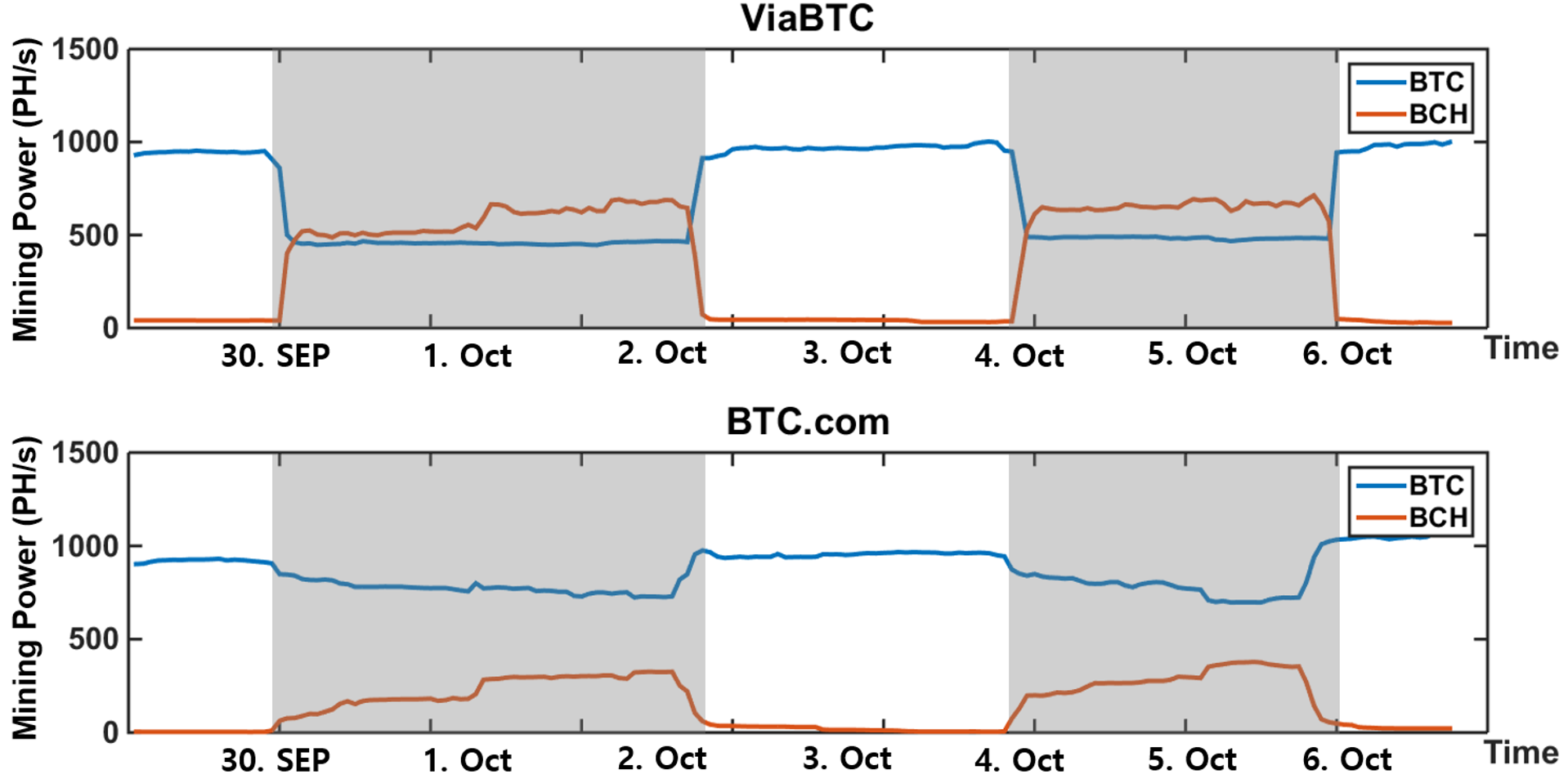
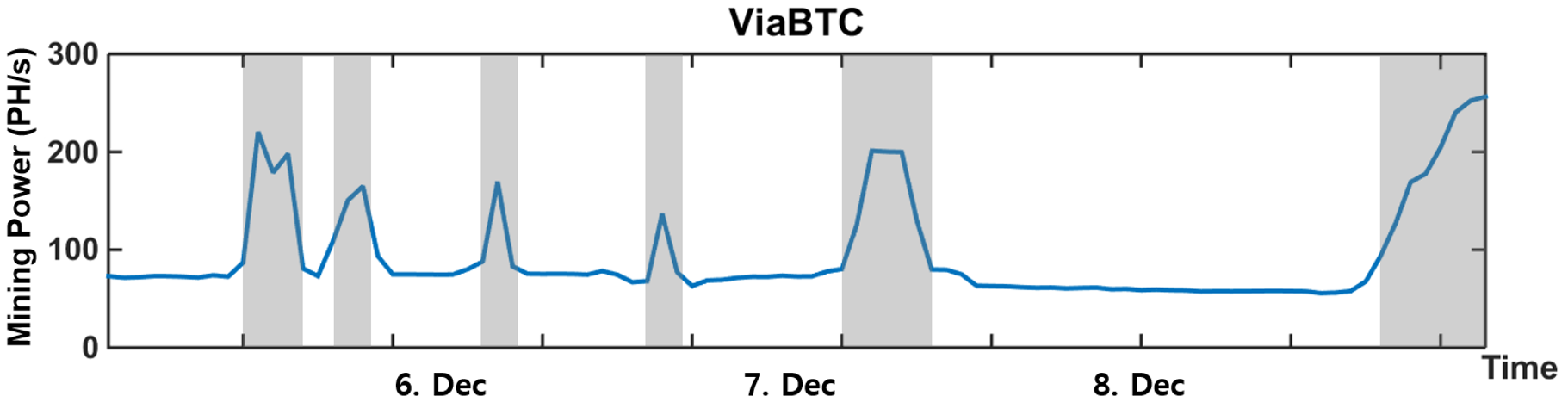
As fickle mining causes a sudden increase in mining power as shown in the grey zones of Figure 1, many blocks were generated quite quickly in the BCH system. For example, in the BCH system, 2016 blocks were generated within only three days in each grey zone. This caused the blockchain of BCH to be thousands of blocks ahead of BTC, and the halving time of the block reward in BCH was brought forward. To address this issue, BCH performed another hard fork on Nov. 13, 2017 [10]. Currently, BCH adjusts the difficulty for each block based on the previous 144 blocks as a moving window [11]. To determine if it is possible that miners conduct fickle mining even after the hard fork of Nov. 13, 2017, we investigated the BCH mining power data of ViaBTC for four days (Dec. 5, 2017 Dec. 8, 2017). Figure 2 represents the BCH mining power data of ViaBTC during this time period; as is evident from the figure, some miners still conduct fickle mining. Because the BCH mining difficulty is more quickly adjusted than before the hard fork of BCH, fickle miners should switch their mining power more quickly than before the hard fork. Indeed, fickle mining can occur in any mining difficulty adjustment algorithm.
III Related work
In this section, we review previous studies related to mining in PoW systems. Kroll et al. considered the Bitcoin mining process as a game among multiple players [12] and showed that a miner possessing 51% mining power can be motivated to disrupt the Bitcoin system. Several works [13, 14] modeled and analyzed a game between two pools that can launch denial of service attacks against each other. Eyal and Sirer introduced the selfish mining strategy, where a malicious miner successfully mines blocks but does not immediately broadcast the blocks; instead, the attacker temporarily withholds the block [15]. Many researchers have intensively studied ways to optimize and extend selfish mining [16, 17, 18, 19]. Bonneau introduced bribery attacks as a way for an attacker to increase her mining power [20]. Lewenberg et al. considered a mechanism of sharing rewards among pool miners as a cooperative game [21]. In 2015, Eyal modeled a game between two pools that execute block withholding (BWH) attacks [22]. As a concurrent work, Luu et al. [23] modeled a power splitting game to find an optimized strategy for a BWH attacker. Kwon et al. [24] proposed a new attack called a fork after withholding (FAW) attack against pools [24]. Also, several works [25, 26] analyzed a transaction-fee regime in PoW systems, where miners receive incentives for mining as transaction fees. Moreover, because many cryptocurrencies are competing with each other, there can be another incentive to execute 51% attacks. Considering this fact, Bonneau revisited the 51% attack with some basic analysis [27].
Recently, Ma et al. [28] considered a mining game of multiple miners and concluded that openness of the Bitcoin system causes the need for vast mining power. Another study [29] examined the relation between the Bitcoin/USD exchange rate and Bitcoin mining power. They first proposed an industry equilibrium model to forecast the mining power depending on the Bitcoin/USD exchange rate. Then, they showed that the real mining power data and simulated mining power according to their model are similar. Our study focuses on the relation between two coins that have compatible PoW mechanisms with each other and the miners’ behavior between two coins. Furthermore, our model can be used to forecast the ratio of mining power between two coins. To the best of our knowledge, this is the first to study the effects of fickle mining.
IV Model
In this section, we formally model a game to represent fickle mining between two coins.
IV-A Notation and assumptions
We consider two coins, and , which have compatible PoW mechanisms with each other. In this case, a miner with a hardware device can alternately conduct mining of and ; that is, he can conduct fickle mining between them. Meanwhile, a -faction can stick to -mining rather than fickle mining or -mining to maintain its own coin, and the set of -factions sticking to -mining is denoted by . For example, in the case where BCH is , BITMAIN [30], one of the main supporters of BCH, may belong to . We aim to formalize a game considering the fickle mining and .
The proposed game consists of many players (i.e., miners), where the set of all players is denoted by Player chooses one of three strategies, : Fickle mining (), -only mining (), and -only mining (). The payoff function of player is denoted by which we will formally define later as well as fickle mining. We also define three sets , , and , indicating a set of players who conduct fickle mining, -only mining, and -only mining, respectively. Note that is a subset of because players in always choose strategy . The sum of mining powers in and is regarded as 1; mining power of a coin is expressed as a ratio to the total mining power. The mining power possessed by player is denoted by and the total computational power possessed by is denoted by We also define as the maximum of Moreover, because our game analysis result would depend on the computational power possessed by players, we use the notation to refer to the game, where indicates a vector of computational power possessed by players except for (i.e., ). Lastly, we denote the total mining power of , , and as (i.e., ), (i.e., ), and (i.e., ), respectively. Observe that and Namely, represents the full status of mining powers where is not less than .
For the analysis of the game, we assume the following:
Assumption 1.
A miner conducts either only or -mining (not both) at each time instance; for example, an ASIC miner cannot execute both BTC and BCH mining simultaneously. However, their choices can be time-varying; that is, miners can change their coin to mine.
Assumption 2.
The price of 1 is equal to that of . We assume that without loss of generality. In addition, rewards for mining a block in both coins are 1 and 1 , respectively.
Assumption 3.
In both and systems, mining difficulties are adjusted to maintain the average period of generating a block as the same specific time period, which we denote by 1 time and regard as a time unit; for example, 1 = 10 minutes in the Bitcoin system. Furthermore, we consider a generalized model in which mining difficulties of and are adjusted in proportion to the mining power for the previous time window, and we consider a normalized difficulty. Thus, if mining power has been engaged in coin mining, the mining difficulty would be More precisely, in our model, the coin mining difficulty decreases and increases again, considering the generation time of a specific number of blocks since the last update of coin mining difficulty. In particular, for the mining difficulty of we denote the number of considered blocks when the -mining difficulty decreases and increases as and , respectively.11 1 In Section VI, we will show that our results can be applied to the coin system regardless of the mining difficulty adjustment algorithm of . Note that and cannot be zero. In the case of BTC and Litecoin, and are 2016.
As described previously, a fickle miner may change the preferred coin when the coin mining difficulty changes. Here we define fickle mining formally.
Definition IV.1 (Fickle mining).
Let and denote the and -mining difficulties, respectively. If or when or is updated, fickle miners () decide to conduct -mining until or is adjusted again. Otherwise, they conduct -mining.
We also emphasize that if is 0, no miner engages in fickle mining, and mining powers of and are stably maintained. On the other hand, if is , only -factions would conduct -mining after an increase in the mining difficulty of In other words, in this case, only the factions remain as loyal miners for Therefore, if the number of such factions () is small, the state would be a lack of loyal miners. Note that loyal miners refer to players who continue to conduct -mining even after an increase in -mining. In particular, if all -factions stop -mining for higher payoff (i.e., ), is 0, and no player conducts -mining after an increase in the mining difficulty of Note that the -mining difficulty cannot decrease in this case because cannot be zero. Therefore, the case indicates the complete downfall of while only survives.
Parameters used in this paper are summarized in Table I. The last parameter in the table will be introduced later.

| The set of -factions sticking to mining to maintain their own coin | |
| The set of all players | |
| Player ’s strategy | |
| Player ’s payoff | |
| , , | Fickle, -only, -only mining |
| , , | The set of players with , , |
| Computational power of player | |
| Computational power possessed by | |
| The maximum of | |
| The vector of computational power possessed by players in | |
| The game of players and with computational power and | |
| The total computational power fraction of , , | |
| The relative price of to | |
| The time unit representing the average period of generating one block | |
| The number of considered past blocks when the mining difficulty of decreases or increases | |
| The mining difficulty of , | |
| The set of all Nash equilibrium in |
Illustration of fickle mining.
Figure 3 illustrates
a stream of mining power in and , as well as the mining difficulty of over time, caused by the strategies of players.
- Time : At the beginning, and mining powers are used for and -mining, respectively.
- Time : The mining difficulty of decreases because it is relatively difficult to find PoWs with mining power.
At the moment, shifts from to , and each of and mining powers is used for and -mining, respectively.
- Time : Because the mining difficulty of is again adjusted (increases) after blocks are found in the system since the last adjustment of the mining difficulty of ,
the mining difficulty of would increase after time since it takes to find one valid block on average.
Then, shifts again from to and conducts -mining until the mining difficulty of decreases.
- Time : Until when the mining difficulty of decreases after blocks are found in the system,
would conduct -mining (for time).
- This process is continually repeated.
IV-B Payoff function
Next, we describe payoff functions for our game model. All payoffs are expressed as a unit of and are calculated as a profit density, which is defined as an average earned reward for time divided by the player’s mining power. In other words, if player earns a reward for 1 time on average, the payoff would be Player ’s payoff function is expressed as follows:
| (1) |
where indicates other players’ strategies. Here, it suffices to define in the range , and respectively; for example, would be defined when (i.e, a fickle miner exists, and ).
First, we define the payoff for a player in . As shown in Figure 3, conducts -mining for time. Therefore, a player in earns the profit per 1 time on average for time. After that, conducts -mining for time during which a player in earns the following profit per 1 time on average:
|
|
(2) |
The above formulation is due to the fact that mining powers and engage in -mining for and times, respectively, and thus, the second factor in the right-hand side of (2) represents an inverse number of the mining difficulty of . Consequently, the payoff of a player in can be expressed as
|
|
where
Next, we provide payoffs and as follows:
where we observe that a player in earns the profit per 1 for time and profit per 1 for time, on average.
V Game analysis
In this section, we analyze Nash equilibria and dynamics in game
V-A Equilibrium in game
Characterization of equilibria. Before finding Nash equilibria of we define a pure Nash equilibrium.
Definition V.1 (Pure Nash equilibrium).
A strategy vector is a Nash equilibrium if
At an equilibrium, all rational players would not change their strategy, that is, and are not updated. We map a strategy vector to state and denote by the set of all Nash equilibria in We first determine the dynamics of player with small through Lemma V.1 to establish the characterization of
Lemma V.1.
Note that is for a small value of while is 0 for a large value of The above lemma implies that, considering miners with small computational power, if a Nash equilibrium exists, only would remain as loyal miners to in the equilibrium. This is because would continually change when is greater than From Lemma V.1, we can characterize the set as stated in Theorem V.2. We present the proof of Lemma V.1 and Theorem V.2 in Appendix A.
Theorem V.2.
There is such that, when the set is as follows.
|
|
where
and range between 0 and 1.
As described above, Theorem V.2 shows that, in a game where players except for possess small computational power, there exist only Nash equilibria where the -factions sticking to -mining are loyal miners for . In the case where is small, we can certainly see that the overall health of the system would be weakened in terms of scalability, decentralization, and security, which will be discussed in more detail in Section VII-A. Indeed, even if is large, the case where is equal to would make the system significantly centralized because only a few players possessing large power are loyal miners to (this example is presented in Section VII-B). In particular, if is empty, no miner exists in the system in all Nash equilibria. Remark that this case indicates the complete downfall of As a result, Theorem V.2 implies that fickle mining can be dangerous.
When players possess infinitesimal mining power. Under the game , it is not easy to analyze movement of state (this movement will be used for data analysis in Section VII) due to a large degree of freedom in . Thus, we further assume that players except for (i.e., ) possess infinitesimal computational power (i.e., ). We show that this assumption is reasonable by analyzing the real-world dataset in the Bitcoin system (see Section VI). We again study the equilibria of in this case.
Theorem V.3.
When players except for possess infinitesimal mining power, the set is as follows.
| (3) |
Here, and are defined in Section V-B.
We present the proof of Theorem V.3 in Appendix B. Comparing with Theorem V.2, the state also becomes another Nash equilibrium when the computational power possessed by players (except for ) is infinitesimal. Note that this state indicates the stable coexistence of and Indeed, when is closer to 0, the difference among payoffs of players in , , and would also be closer to 0 at the state . Therefore, under the assumption that players possess infinitesimal power, payoffs of players in , , and are the same at the state while the mining difficulties of and are maintained as and , respectively. Meanwhile, at the remaining equilibria except for the state , only the -factions conduct -mining after the -mining difficulty increases. In particular, if no -faction sticking to -mining exists, loyal mining power to is 0 in the Nash equilibria. Note that, in this case, and would continuously conduct -mining, because the mining difficulty of has not decreased after the previous increase in difficulty. These players would not also change their strategy because the mining difficulty of increases to a significantly high value due to the heavy occurrence of fickle mining.
Example. Considering the case we give an example where and the initial mining difficulty of is 0.4. The state is not a Nash equilibrium according to Theorem V.3. Because fickle miners continuously conduct the -mining, the mining difficulty of is maintained as 1, and players in and earn the payoff of 1. If a player moves into , the player would earn for a while in the beginning. However, because the mining difficulty of decreases after finds several blocks, the player who moves to would eventually earn consistently. Note that the time duration in which the mining difficulty of is close to 0 is negligible compared to the time duration in which the mining difficulty of is 0.2. Therefore, the payoff of is and rational players tend to move to due to the higher payoff. This means that the state is not a Nash equilibrium.
V-B Dynamics in game
In this section, we analyze dynamics in the game and study how a state can reach an equilibrium.


Best response dynamics. In game , point reaches either of the two types of Nash equilibria: the stable coexistence of two coins and the lack of loyal miners to Figure 4 represents dynamics in game , where horizontal and vertical axes are and values, respectively. A line, , represents
| (4) | ||||
On the line, the payoffs of (i.e., ) and (i.e., ) are the same. In addition, the line does not intersect with the line and has an intersection with the line for , where is a solution of equation for . The equation has only one solution , and it is between 0 and . Another line, , represents
| (5) | ||||
and the payoffs of (i.e., ) and (i.e., ) are the same on the line. The line does not intersect with the line for and has an intersection with the line . Moreover, it is most profitable among the three strategies to continually conduct -mining () in a zone above . We let this zone be . In the zone below , it is most profitable to continually conduct -mining (), and the zone is denoted as . In the zone between and , fickle mining () is the most profitable, and this zone is denoted as . Note that the range of zones changes if the coin price changes because boundaries are functions of
The moving direction of point is expressed as a red arrow in Figure 4. For ease of reading, we express directions in which values and increase () or decrease () as . For example, indicates the direction in which both values, and , increase. In , is the most profitable strategy, and thus every point in moves in the direction . In , because is the most profitable strategy, every point moves in the direction . Finally, in , as is the most profitable strategy, every point in moves in the direction . Figure 4 shows the directions in the three zones (, , and ).
2D-Illustration of movement towards equilibria. To determine which equilibrium can be reached within each zone, we represent all Nash equilibria in game depending on a value of as yellow points and line in Figure 5. In the figure, the red dash lines represent for each case. As described in Section V-A, there are two types of equilibrium points: 1) a lack of loyal miners and 2) stable coexistence of two coins. The equilibrium point representing a lack of loyal miners would be located on a red dash line , and we can see that all cases have this equilibrium. For Cases 1, 2, and 3, the second type of equilibrium (i.e., ) representing stable coexistence of two coins is also found. A point moves in the direction depending on its zone. In the meantime, if the point meets the line then the point moves toward an equilibrium located on the line as shown in Figure 5. In particular, the value of in the equilibrium on the red dash line representing Case 3 is denoted by , where the equilibrium is the intersection point between and the red dash line. Note, a point in would not meet a red dash line because the point in moves in the direction and can always be above the red dash line. Therefore, such points in are likely to reach the stable coexistence of and However, some points (near to ) in can also move into when more miners of than that of revise their strategies, and then it is possible to reach the equilibrium, representing a lack of loyal miners to .
VI Application to Bitcoin System
In this section, we apply our game model to Bitcoin as a case study. Specifically, we consider game when players possess sufficiently small mining power. To see if this assumption is reasonable, we investigate the mining power distribution in the Bitcoin system, referring to the power distribution provided by Slush [31]. The distribution is depicted in Figure 6 where the -axis represents the range of the relative computational power and the -axis represents the number of miners possessing computational power in the corresponding range. The figure shows that 1) most miners possess sufficiently small mining power, and 2) even the maximum computational power is less than Note that BITMAIN’s is about as of Dec. 2018. Moreover, even though mining pools currently possess large computational power, the miners in pools can individually decide which coin to mine. We also recognize the distribution of computational power is significantly biased toward a few miners, as shown in Figure 6. However, this fact does not imply that is large. Referring to the data provided by Slush, is only about 0.05, where this value is equivalent to that for the case where all miners possess computational power.22 2 We calculated this assuming that other pools have the computational power distribution similar to Slush. Therefore, most miners (and most mining power) would follow dynamics of game . As a result, we can apply game to the practical systems.

Now, we describe how game is applied to the Bitcoin system. As described in Section II, Bitcoin was split into BTC and BCH in Aug. 2017. Thus, we can map BTC and BCH to and , respectively. For the mining difficulty adjustment algorithm of BCH, we should consider two types of BCH mining difficulty adjustment algorithms: those that BCH have before and after Nov. 13, 2017. This is because the mining difficulty adjustment algorithm of BCH changed through a hard fork of BCH (on Nov. 13, 2017).
Before Nov. 13, 2017. First, we consider the mining difficulty adjustment algorithm of BCH before Nov. 13, 2017. In this algorithm, not only the mining difficulty is adjusted for every 2016 block, but also EDA can occur as described in Section II. Note that EDA occurs if the mining is significantly difficult in comparison with the current mining power, i.e., EDA is used only for decreasing the BCH mining difficulty. Therefore, the value of is 2016 because the BCH mining difficulty can increase after 2016 blocks are found. Meanwhile, when the BCH mining difficulty decreases, the value of varies depending on and , ranging between 6 and 2016. Thus, we can consider the expected number of blocks found until the mining difficulty decreases (i.e, the mean of denoted by ) instead of , and as a function of and would continuously vary from 6 to 2016. If is 0, is 2016 because EDA does not occur, and if is 0, is 6.
As a result, the Bitcoin system before Nov. 13, 2017 can be where substitutes for This game has also Nash equilibria and dynamics as shown in Figure 4 because is a continuous function of and
After Nov. 13, 2017. Next, we consider the Bitcoin system after Nov. 13, 2017. In this case, the BCH mining difficulty adjustment algorithm is different from that assumed in our game because the mining difficulty is adjusted for every block by considering the generation time of the past 144 blocks as a moving time window. Despite that, game can be applied to this system. Indeed, in general, our results for game would appear in the Bitcoin system regardless of the BCH mining difficulty adjustment algorithm, shown below.
Theorem VI.1.
Because the current BCH mining difficulty is adjusted every block, Theorem VI.1 implies that results for game is also applied to the current Bitcoin system even though the BCH mining difficulty adjustment algorithm changed. The proof of Theorem VI.1 is presented in Appendix C.
| (a) |

|
| (b) |

|
| (c) |

|
| (d) |

|


VII Data analysis
VII-A BTC vs. BCH
We analyze the mining power data in the Bitcoin system to identify to which equilibrium the state has been moving. Moreover, through this data analysis, we can find out empirically how much our theoretical model agrees with practical results. For data analysis of the Bitcoin system, we collected the mining power data of BTC and BCH from the release date of BCH (Aug. 1, 2017) until the time of writing (Dec. 10, 2018) from CoinWarz [32]. Figure 7a represents the mining power history of BCH, where the mining power is expressed as a fraction of the total power in BTC and BCH, i.e.,
In addition, we represent the data history of a ratio between difficulties of BCH and BTC (i.e., ) and a relative price of BCH to that for BTC (i.e., ) in Figure 7b and 7c, respectively. The price of BCH is depicted as a yellow line in Figure 7c (see the left -axis). Moreover, Figure 7c represents the relative BCH mining profitability () to the BTC mining profitability as a purple line, and the black dashed line represents (see the right -axis for the two lines). For this profitability, to increase reliability of data, we collected the daily BCH profitability from CoinDance [33], and thus a purple point is a data captured every day. Note that is less than in the case where the purple line is above the black dashed line. Figure 7d simultaneously shows all data histories (except for the BCH mining profitability) presented in Figure 7a7c. In Figure 7, the data from Dec. 2017 to Nov. 2018 are omitted because they are similar to the data for Dec. 2018. Figure 8a8i correspond to parts (1)(9) of Figure 7, respectively, where the area of three zones has changed because the relative price of BCH to that for BTC has fluctuated quite frequently.
As another case study, we examine the mining power data of Bitcoin ABC and Bitcoin SV from Nov. 1, 2018 to Dec. 20, 2018 to analyze a special situation where suddenly increases due to the “hash war” caused by a hard fork in the BCH system. We describe this in Section VII-B.
Methodology. We first describe how to determine and of each state. According to the definition of fickle mining (Definition IV.1), fickle miners would conduct BCH mining from when changes to a value less than to when changes to a value greater than This is because is always less than and greater than (see Figure 7d). Therefore, Figure 7a represents the value of during the period. We indicate the fickle mining periods in gray before the hard fork of BCH (Nov. 13, 2017) in Figure 7. Figure 7d shows that changes to a value less than and greater than at the start and end of these periods, respectively. As a result, in Figure 7a, we can find out the value of for the gray colored periods and the value of for non-colored periods. Here, we can see that the mining power of BCH has fluctuated considerably when the ratio of the BCH mining difficulty to the BTC mining difficulty () changes to a value less than . Moreover, when the coin mining difficulties do not change while BCH mining is more profitable than BTC mining, large peaks (i.e., a sudden increase) do not appear. This fact is confirmed, referring to the purple line in non-colored zones (e.g., part (3) in Figure 7c). As a result, we can consider that those fluctuations occur due to fickle miners between BTC and BCH.
If a miner switches the coin to mine without changes in the coin mining difficulty, this implies that the miner’s strategy changes (e.g., from to ). From the method described above, we can determine the mining power used for fickle mining and the mining power used for BCH-only mining. The points and directions are marked roughly in Figure 8. The red arrow represents movement in agreement with our analysis, whereas the black arrow represents movement deviating from our analysis.
The beginning of the game. In Figure 7-(1), the status point is initially in , and then it moves to as shown in Figure 8a, as the BCH mining power decreases.
Towards the lack of BCH loyal miners. In Figure 7a-(2), two peaks occur when the BCH mining difficulty decreases to values less than and these peaks appear in the gray colored periods. Therefore, we can know that these peaks occur due to fickle miners. The first peak indicates that more and more miners started fickle mining (i.e., increase in ). This is because the upflow of the first peak is less steep than that for other peaks, and the downflow of the first peak is steeper than the upflow of the first peak, indicating that increases from near 0 up to near 0.4. Furthermore, one can see that increased at the beginning of Figure 7a-(2). Remark that Figure 7a shows the value of in a non-colored zone. In addition, the BCH mining power in the valley between two peaks of Figure 7a-(2) is greater than the mining power at the end of Figure 7a-(1). This fact shows again that increased at the beginning of Figure 7a-(2). After that, because the end of Figure 7a-(2) is less than the valley between the two peaks of Figure 7a-(2), we can know that decreased while increased in Figure 7a-(2). Figure 8b represents these movements described above.
In the beginning of Figure 7a-(3), slightly increases, and it does not correspond with our model; we regard this as a momentary phenomenon because of a decrease in the BCH mining difficulty. Figure 7b shows that the BCH mining difficulty decreased at the beginning of the part (3). However, even though the BCH mining difficulty decreased, peaks due to fickle mining do not appear because the relative BCH mining difficulty did not decrease to a value less than as shown in Figure 7d. As a result, as can be seen in Figure 8c, the point moves alternatively between and . One can see that decreased compared with the mining power in the peaks of Figure 7a-(4) and the peaks in Figure 7a-(2); this might be because the moving direction in is .
Next, the peaks in the period presented in Figure 7a-(4) appeared due to fickle miners because the BTC mining difficulty increased. We can check that in the period decreased to a value less than through Figure 7d. Note that the fact that the BTC mining difficulty increased makes the value of decrease. Indeed, the two peaks of the period show that decreases and then increases because is represented in the period of Figure 7a. This may be explained according to our model as follows: the state was near to the boundary between and at the beginning of Figure 7-(4), and then the state entered while moving in the direction (the moving direction in ) as in Figure 8d. Then, the state in moved in the direction in agreement with our game, and one can see that the third peak (i.e., the beginning of the second gray colored zone in Figure 7a-(4)) is higher than the second peak. After that, decreases (see the second gray colored zone in Figure 7a-(4)), showing a deviation from our model, which is indicated by the black arrow in Figure 8d. Indeed, considering this case as well as Figure 7-(3), we observe such noises in the case where changes to a value close to
Next, as shown in Figure 8e, the point in moves in the direction again because peaks in Figure 7a-(5) are higher than that for Figure 7a-(4). Moreover, in Figure 7c-(4)(6), is roughly decreasing and even drops to about 0.055 in a few cases. In the meantime, the point passes
Because the state entered , starts to decrease, moving in the direction (as shown in Figure 8f). Therefore, the first peak in Figure 7a-(6) is smaller than the last peak in Figure 7a-(5). Then, because the second peak is higher than the first peak in Figure 7a-(6), one can see that the point moved in the direction in in agreement with our model, which is, in turn, depicted in Figure 8f.
As can be seen in Figure 8g, first increases in Figure 7a-(7), and the point enters ; this is a deviation from our analysis, which may be explained because the BCH mining is momentarily more profitable than the BTC mining at the time. Here, we can see again the noise in the case where the value of is close to However, decreases again in agreement with our model. In addition, one can see that decreases in the meantime because the starting height of the peak in Figure 7a-(8), which is marked by a red point, is less than that of the final peak in Figure 7a-(6). Therefore, the point in moved in the direction and entered , conforming with our analysis.
Then, in the second week of Nov. 2017, the price of BCH was suddenly pumped ( in some cases). Therefore, widens in Figure 8h. Also, the point in continuously moves in the direction , and even increases to over 0.5. It can be seen that the peak in Figure 7-(8) has a right-angle trapezoid with a positive slope, which indicates that continuously increases even though it was already high. From the history, we observe that the Bitcoin system often reaches the lack of BCH loyal miners. However, a breakthrough exists even in this bad situation. If continuously increases, widens, and it makes the state enter and reach close to the coexistence equilibrium. As a result, considering the state of Bitcoin as of Nov. 13, 2017, had to increase to a minimum of 0.5 in order for the mining power engaging in fickle mining to decrease.
Close to coexistence. However, at the end of Figure 7-(8), another hard fork occurred in BCH for updating the difficulty adjustment algorithm, and this influenced the status as an external factor. Consequently, the point jumped into due to this hard fork as shown in Figure 8h. After the hard fork, the point moves in the direction , reaching close to coexistence. This is shown by this fact that fluctuations became stable more and more in the beginning of Figure 7a-(9). Note that peaks occur in a short time after the hard fork because the BCH mining difficulty is quickly adjusted. Even though the state has been close to coexistence, fickle mining is still possible and observed as described in Section II. In addition, as the price continuously changes, the point sometimes enters where fickle mining increases, alternating up and down in the red semicircle in Figure 8i. In other words, fickle mining will not completely cease. Therefore, if the Bitcoin state largely deviates from the equilibrium of coexistence due to external factors such as a sudden change in prices, then it is still possible to reach the lack of BCH loyal miners.
Influence of the lack of BCH loyal miners. We observe that the Bitcoin system suffered from the lack of BCH loyal miners before Nov. 13, 2017. Consequently, the BCH transaction process speed periodically became low, and it even took about four hours to generate one block in some cases. Moreover, we can see that BCH was significantly centralized during the period in which the BCH mining difficulty is high. For example, when considering blocks generated from Oct. 2 to Oct. 4, only two accounts generated about 70 % of blocks and there were only five miners who conducted BCH mining. We note that, in blockchain systems using a PoW mechanism, high mining power is an essential factor for high security blockchain systems. In practice, BCH before Nov. 13, 2017 was susceptible to double spending attacks with only 12% of the total computational power in the Bitcoin system. There is also selfish mining [15], which makes the attacker unfairly earn the extra reward while others suffer a loss. Because of a decrease in these attacks can be executed with relatively small mining power. As a result, fickle mining, which heavily occurred before Nov. 13, 2017, weakened the performance, decentralization level, and security of the BCH system.
Influence of the hard fork of BCH. Next, we discuss why Bitcoin moved toward different equilibria before and after Nov. 13, 2017. First, in the Bitcoin system before Nov. 13, 2017, considerably increased as can be seen in Figure 7a-(2). Meanwhile, after Nov. 13, 2017, did not considerably increase even though the point passed . This can be attributed to the different difficulty adjustment algorithms before and after Nov. 13, 2017; the mining difficulty of BCH is currently adjusted faster than that before Nov. 13, 2017. Therefore, currently, to conduct fickle mining, miners must switch between BTC and BCH relatively fast; this would make the current fickle mining in the Bitcoin system annoying. Then, can we regard the current state of BCH to be safe if the system avoids external factors such as a sudden change in prices? We delay the answer until Section VIII.
VII-B The ”hash war” between Bitcoin ABC and Bitcoin SV
According to our model, we also describe the “hash war” that recently occurred between Bitcoin ABC (ABC) and Bitcoin SV (BSV), which are derived from the original BCH on Nov. 15, 2018. In this paper, we call ‘Bitcoin ABC’ ABC rather than BCH to avoid confusion with the original BCH even though Bitcoin ABC is currently regarded as BCH [34]. This war was caused by the conflict over a BCH update that adds a new opcode, where the BCH factions split into a reformist group and an opposing group. As a result, this conflict caused the two factions to make their own chain, where the reformist group is the ABC faction led by Roger Ver (the owner of Bitcoin.com [35]) and Jihan Wu (the cofounder of Bitmain and also the owner of BTC.com [9] and Antpool [36]) and the opposing group is the BSV faction led by Craig Wright and Calvin Ayre (the CEO of Coingeek [37]). This split of the original BCH was achieved by a hard fork on Nov. 15, 2018, and each faction wanted its own chain to be the longest chain in order to unify the divided BCH. This fact makes both factions desperately conduct mining of their coins with vast computational power; thus the hash war occurred from Nov. 15, 2018 to Nov. 24, 2018. Such behavior of ABC and BSV factions would influence on a general miner who choose its coin among BTC, ABC, and BSV, and we analyze this situation by dividing into two games: 1) a game between BTC and ABC and 2) another game between BTC and BSV. In both games, became significantly high during the hash war period, and we can consider this situation as Case 4 ().


To analyze a phenomenon that appeared due to the hash war, we collect the data for ABC and BSV. Figure 9 and 10 show the ABC data history from Nov. 1, 2018 to Dec. 20, 2018 and the BSV data history from Nov. 15, 2018 to Dec. 20, 2018, respectively. Note that BSV was released on Nov. 15, 2018. In Figure 9, the mining power of ABC is presented as a relative value to the total mining power of ABC and BTC, and is also presented, where indicates a relative price of ABC to that for BTC. Figure 10 depicts the data history of BSV like Figure 9. These figures show that the state in the two games was above the state during the hash war period.
Moreover, to determine the movement of the state for the hash war period, we investigate the history of ABC computational power distribution among miners from Nov. 1, 2018 to Dec. 20, 2018 and that for BSV from Nov. 15, 2018 to Dec. 20, 2018. This is because it would be hard to determine the movement of the state through just the mining power history (i.e., Figure 9 and 10) because significantly changed during this period. Figure 11 and 12 represent the changes in the mining power distribution of ABC and BSV over time, respectively. To do this, we crawled coinbase transactions and analyzed the number of blocks mined by each miner among previous 100 blocks. In these figures, each miner corresponds to one color, and the length of one colored bar represents the number of blocks generated by the corresponding miner among 100 blocks. Therefore, the number of colors in the entire bar indicates the number of active miners at the corresponding time. Note that only names of ten miners are presented in Figure 11.
First, we consider the game between BTC and ABC. One can see that the state jumps to a point above for the hash war preparation period (from Nov. 13, 2018 to Nov.15, 2018) through Figure 9. Such an increase in the ABC mining power may be explained because the mining power of BSV factions such as CoinGeek, svpool, BMG pool, and Mempool increased from the hash war preparation [38] as shown in Figure 11. In other words, the increase in the ABC mining power for the hash war preparation is because increased. On the other hand, Figure 11 shows that some miners left the ABC system during the war preparation (the colors that appeared at the top of the figure before the war preparation period disappeared from the war preparation period). This fact indicates that the state moves toward the line in the case that is large. Note that the reason why the ABC mining power decreases at the end of the hash war preparation period (i.e., the start of the hash war) is that BSV factions move to the BSV system.
Next, for the hash war period, the ABC mining power increased because the ABC factions such as Bitcoin.com increased their mining power (i.e., increased) [34]. However, there were only a few loyal ABC miners during this period. For example, at the start of the hash war, only five miners exist: Bitcoin.com, BTC.com, AntPool, ViaBTC, and BTC.TOP. Note that all of them are the ABC factions (ViaBTC and BTC.TOP announced that they support ABC [39, 40]). As a result, we can see that this state is close to the state which represents a lack of BCH loyal miners. This state makes the ABC system severely centralized. In particular, one miner (Bitcoin.com) possessed about 60 % of the total computational power in some cases, which indicates the breakage of censorship resistance. Meanwhile, after the hash war (i.e., when is less than ), one can see that more other miners gradually enter the ABC system (see the increase in the number of colors after the hash war in Figure 11). In addition, Figure 9 shows that the state is close to after the hash war. As a result, the state moves as shown in Figure 13.
Second, we describe the game between BTC and BSV through Figure 10 and 12. As shown in Figure 10, the state is above for the hash war period because is significantly high. This fact is also presented in Figure 12. Note that CoinGeek, svpool, BMG, and Mempool are BSV factions. Therefore, the state was close to at the time. Similar to ABC, BSV also suffered from the severe centralization due to a lack of loyal miners. However, the other miners have entered the BSV system after the hash war, and the state became close to . Therefore, Figure 13 represents the state movement, and this result empirically confirms our theoretical analysis.
Here, note that when the state is located above suffers a loss. This fact makes the state would not last for a long time. Therefore, the hash war was also not able to continue for a long time, and the hash war ended with BSV’s surrender [41].
VIII Broader Implications
In this section, we describe broader implications of our game model. More precisely, we first describe the risk of automatic mining, and then explain how one coin can exploit this risk to intentionally steal the loyal miners from other less valued coins with negligible efforts and resources.
VIII-A A potential risk of automatic mining
As described above, the current state of Bitcoin is close to coexistence between BTC and BCH because faster BCH mining difficulty adjustment makes manual fickle mining inconvenient. We introduce another possible mining scheme called automatic mining, which can be less affected by faster mining difficulty adjustment. Automatic mining is designed for miners to automatically switch the coin to mine to the likely most profitable one of the compatible coins by analyzing their mining difficulty and coin prices in real time unlike fickle mining. Here, note that all automatic miners almost simultaneously change their coin when not only mining difficulty but also coin prices changes. Indeed, automatic mining can be considered to be automatically choosing the most profitable one among three strategies, , , and in real time. Automatic mining has been executed in the Bitcoin system [42] and has already become popular in the altcoin system [43]. Indeed, mining power increases and decreases by more than a factor of four in most altcoins several times a day [44]. We describe a simple implementation of automatic mining below.

Currently, many mining pools, including BTC.com, Antpool, and ViaBTC, support interactive user interfaces for switching the coin to mine by just clicking one button. Figure 14 represents the one-button switching mining feature provided by Antpool. This feature makes automatic mining easier without technical difficulties in implementing this approach. For example, a miner can conduct automatic mining in Antpool as follows.
- 1.
First, the miner saves an HTTP header with its cookies to maintain the login session.
- 2.
- 3.
If BTC mining is more profitable than BCH mining, the miner sends an HTTP request, which includes the saved HTTP header and data for switching to BTC mining. Otherwise, the miner sends an HTTP request to conduct BCH mining.
- 4.
The above steps are repeated.
As shown in the code [47], this automatic mining can be executed within about 50 lines in Python.
Large-scale automatic mining makes the state of the coin system enter . As a simple example, we can consider an extreme case wherein the entire computational power is involved in automatic mining. In this case, any initial state except for immediately reaches the equilibrium as soon as all miners start automatic mining. This is because all automatic miners should simultaneously choose the same coin and would eventually mine when the mining difficulty of increases.
Then, we have the following question: What ratio of automatic mining power is needed to reach the lack of -loyal miners? As shown in Figure 4, the state cannot be in when is not less than Therefore, where would move in the decreasing direction of . Further, even manual miners who do not conduct automatic mining would prefer rather than at states in where because -only mining is more profitable than -only mining at the states; loyal miners of should generate blocks with high difficulty. Therefore, when a fraction of the total mining power is involved in the automatic fickle mining, the state moves towards a lack of -loyal miners. As of Dec. 2018, because in the Bitcoin system is about 0.05, if 5% of the total mining power in the Bitcoin system is involved in automatic mining, the automatic miners would conduct (automatic) fickle mining and the state would enters . Note that if automatic miners of which the total mining power is 5% conduct -only (or -only) mining, the state would enter (or ). This is contradiction because the automatic miners should choose the most profitable strategy. As a result, when only 5% of the total mining power is involved in the automatic mining, the number of BCH loyal miners decreases and the BCH system is finally becoming more centralized.
VIII-B Injuring rivalry coins
In Section VI, we explained how our game can be applied to the Bitcoin system regardless of the BCH mining difficulty adjustment algorithm. To generalize our game model, we here consider two types of possible mining difficulty adjustment algorithms: The first type of algorithm is to adjust the mining difficulty in a long time period (e.g., two weeks) while the second type of algorithm is to adjust the mining difficulty every block or in a short time period in order to promptly respond to the changes in the mining power. In the real-world, both types of these mining difficulty adjustment algorithms are mostly used. For example, BTC and Litecoin are the cryptocurrency systems using the first type, while many altcoins including BCH, Ethereum (ETH), and Ethereum Classic (ETC) are currently using the second type.
We can generalize our game model to any coin system satisfying the following conditions.
- 1.
Two existing coins share the same mining hardware.
- 2.
The more valued coin between those coins has the first type of mining difficulty adjustment algorithm.
We note that there is no restriction on the mining difficulty adjustment algorithm for the less valued in our game model . When has the first type of mining difficulty adjustment algorithm, our model can be applied according to Section IV. Note that we modeled our game in Section IV, assuming that has the first type of mining difficulty adjustment algorithm. In addition, in Section VI, we described why our game can be applied to when has the second type of mining difficulty adjustment algorithm. Therefore, regardless of mining difficulty adjustment algorithm, in the coin system satisfying the above two conditions, the -loyal miners would leave if at least fraction of the total mining power is involved in automatic mining.
Next, we explain how the more valued coin can steal loyal miners from the other less valued rivalry coin. If utilizes the first type of mining difficulty adjustment algorithm, the number of -loyal miners would naturally decrease due to the automatic mining. Again note that this situation periodically weakens the health of the system in terms of security and decentralization. On one hand, if has a mining difficulty adjustment algorithm different from the first type (i.e., different from that in Assumption 3), our game model may not be applied. For example, when considering the Ethereum system consisting of ETH and ETC, ETH corresponding to has a different difficulty adjustment algorithm from that which we assumed in our game. In this case, even if the complete downfall of (e.g., ETC) may not occur and the mining power of and would fluctuate heavily. Therefore, to follow our game and so steal the loyal miners from , should change its mining difficulty adjustment algorithm through a hard fork. We can see that some cryptocurrency systems (e.g., BCH, ETH, and ETC) have often performed hard forks to change their mining difficulty adjustment algorithms [48, 49, 50]. This indicates that cryptocurrency systems can practically update their mining difficulty adjustment algorithms if needed.
In conclusion, if the mining difficulty adjustment algorithm for is changed to the first type of mining difficulty adjustment algorithms, a lack of loyal miners for might be reached due to automatic mining.
IX Discussion
In this section, we first discuss how can maintain its loyal miners and consider environmental factors that may affect our game analysis results.
IX-A Maintenance of -loyal miners
As described in Section VIII-B, cannot prevent the rivalry coin from stealing loyal miners by changing its difficulty adjustment algorithm alone. Surely, the most straightforward way to avoid the risk is to not use the mining hardware compatible with . That is, a proprietary mining algorithm, requiring customized mining hardware which is not compatible with , should be introduced for . However, this solution is not applicable in practice for small and medium-sized mining operators because it is expensive to develop customized mining hardware (e.g., ASICs). In fact, because many altcoins use a mining algorithm that can be implemented in CPU or GPU, automatic mining endangers their mining power, weakening their security.
The second way is to use auxiliary proof-of-work (or merged mining), which makes a miner conduct mining more than two coins at the same time [51]. Therefore, our first assumption in Section IV is not satisfied by merged mining, and our game results would not be applied. This is also regarded as a potential solution to 51% attacks because it significantly increases mining power of altcoins [52]. However, despite of such definite advantages, most projects do not adopt merged mining because of following reasons: It is complex to implement merged mining, and miners should do additional work [52].
The another way is to increase the price of through price manipulation. However, as far as we know, the problem of maintaining the increased coin price through price manipulation is not well-studied. Moreover, we can consider a way to increase the relative incentive of mining to mining, where it can be achieved by increasing the block reward or decreasing the average time of block generation. Even though this method may help prevent the rivalry coin from stealing loyal miners, it would cause other side effects such as inflation or the increase in fork rate [25, 18].
Lastly, can change its consensus protocol, the PoW mechanism, to another protocol. However, this process would not be supported by existing miners in . For example, Ethereum is planning to switch from a proof-of-work mechanism to a proof-of-stake mechanism for several years. However, note that if the consensus protocol is just changed through a hard fork, the existing miners may leave because they can lose their own merits (e.g., powerful hardware capability) for mining .
IX-B Environmental factors
In practice, miners’ behavior can deviate from our model because of the following environmental factors.
Not all miners are rational. First, miners are not always rational or wise. Even if fickle mining or mining is more profitable than mining, some miners may be reluctant to engage in fickle mining or mining because they may not recognize the profitability in doing so. However, our data analysis confirms that most miners are rational. In addition, if miners use the automatic mining function, they would always follow the most profitable strategy.
Some miners consider the long-term price of coins. Because price prediction is significantly difficult [53], we believe that most miners behave depending on the short-term price of a coin rather than the long-term price. For example, who could have predicted the hash war between ABC and BSV in advance? Therefore, as can be seen from the history of the Bitcoin system, most miners behave depending on short-term profits. To model more realistic and general situations, our model considered both rational miners who are interested in short-term profits and factions () which are interested in long-term profits.
Some miners prefer the stable coexistence of coins. Some miners may want the stable coexistence of coins for coin market stability, and they may try to reach the equilibrium representing the coexistence of coins regardless of their profits. If the fraction of such miners is large, a state would move to the equilibrium regardless of its zones. Based on historical observations of the Bitcoin system, however, the fraction of these miners seems unlikely to be high in the real-world.
X Conclusion
In this study, we modeled and analyzed the game between two coins for fickle mining, and our results imply that fickle mining can lead to a lack of loyal miners in the less valued coin system. We confirm that this lack of loyal miners can weaken the overall health of coin systems by analyzing real-world history. In addition, our analysis is extended to the analysis of automatic mining, which shows a potentially severe risk of automatic mining. As of Dec. 2018, BCH’s loyal miners would leave if more than about 5% of the total mining power in BTC and BCH is involved in automatic mining. Moreover, we explained how one coin can steal the loyal miners from other less valued rivalry coins in the highly competitive coin market by generalizing our game model. We believe that this is one of the serious threats for a cryptocurrency system using a PoW mechanism.
Acknowledgment
We are very grateful to the anonymous reviewers and Andrew Miller, the contact point for major revision of this paper.
References
- [1] S. Nakamoto, “Bitcoin: A peer-to-peer electronic cash system,” 2008.
- [2] “Proof of Work.” https://en.bitcoin.it/wiki/Proof_of_work, 2017. [Online; accessed 30-Oct-2017].
- [3] “Bitcoin Cash.” https://www.bitcoincash.org/, 2018. [Online; accessed 31-May-2018].
- [4] Jimmy Song, “Bitcoin Cash: What You Need to Know.” https://medium.com/@jimmysong/bitcoin-cash-what-you-need-to-know-c25df28995cf, 2017. [Online; accessed 31-Jun-2018].
- [5] Mengerian, “Bringing Stability to Bitcoin Cash Difficulty Adjustments.” https://medium.com/@Mengerian/bringing-stability-to-bitcoin-cash-difficulty-adjustments-eae8def0efa4, 2017. [Online; accessed 25-Jul-2018].
- [6] “Segregated Witness.” https://en.bitcoin.it/wiki/Segregated_Witness, 2018. [Online; accessed 28-Dec-2018].
- [7] Jimmy Song, “Bitcoin Cash Difficulty Adjustments.” https://medium.com/@jimmysong/bitcoin-cash-difficulty-adjustments-2ec589099a8e, 2018. [Online; accessed 31-Jun-2018].
- [8] “ViaBTC.” https://pool.viabtc.com/, 2018. [Online; accessed 30-May-2018].
- [9] “BTC.com.” https://pool.btc.com/pool-stats, 2018. [Online; accessed 30-Jun-2018].
- [10] “Bitcoin Cash Hard Fork Plans Updated: New Difficulty Adjustment Algorithm Chosen.” , 2017. [Online; accessed 10-Dec-2017].
- [11] “Bitcoin Cash’s New Hard Fork - How The New Difficulty Algorithm Will Work.” https://www.justcryptonews.com/194/bitcoin-cashs-new-hard-fork-how-new-difficulty-algorithm-will-work, 2017. [Online; accessed 10-Dec-2017].
- [12] J. A. Kroll, I. C. Davey, and E. W. Felten, “The economics of bitcoin mining, or bitcoin in the presence of adversaries,” in Proceedings of WEIS, vol. 2013, p. 11, 2013.
- [13] B. Johnson, A. Laszka, J. Grossklags, M. Vasek, and T. Moore, “Game-theoretic analysis of DDoS attacks against Bitcoin mining pools,” in International Conference on Financial Cryptography and Data Security, pp. 72–86, Springer, 2014.
- [14] A. Laszka, B. Johnson, and J. Grossklags, “When bitcoin mining pools run dry,” in International Conference on Financial Cryptography and Data Security, pp. 63–77, Springer, 2015.
- [15] I. Eyal and E. G. Sirer, “Majority Is Not Enough: Bitcoin Mining Is Vulnerable,” in International Conference on Financial Cryptography and Data Security, Springer, 2014.
- [16] A. Sapirshtein, Y. Sompolinsky, and A. Zohar, “Optimal selfish mining strategies in bitcoin,” in International Conference on Financial Cryptography and Data Security, pp. 515–532, Springer, 2016.
- [17] K. Nayak, S. Kumar, A. Miller, and E. Shi, “Stubborn mining: Generalizing selfish mining and combining with an eclipse attack,” in Security and Privacy (EuroS&P), 2016 IEEE European Symposium on, pp. 305–320, IEEE, 2016.
- [18] A. Gervais, G. O. Karame, K. Wüst, V. Glykantzis, H. Ritzdorf, and S. Capkun, “On the security and performance of proof of work blockchains,” in Proceedings of the 2016 ACM SIGSAC Conference on Computer and Communications Security, pp. 3–16, ACM, 2016.
- [19] R. Zhang and B. Preneel, “On the necessity of a prescribed block validity consensus: Analyzing bitcoin unlimited mining protocol,” in Proceedings of the 13th International Conference on emerging Networking EXperiments and Technologies, pp. 108–119, ACM, 2017.
- [20] J. Bonneau, “Why buy when you can rent? Bribery attacks on Bitcoin consensus,” in BITCOIN ’16: Proceedings of the 3rd Workshop on Bitcoin and Blockchain Research, February 2016.
- [21] Y. Lewenberg, Y. Bachrach, Y. Sompolinsky, A. Zohar, and J. S. Rosenschein, “Bitcoin mining pools: A cooperative game theoretic analysis,” in Proceedings of the 2015 International Conference on Autonomous Agents and Multiagent Systems, pp. 919–927, International Foundation for Autonomous Agents and Multiagent Systems, 2015.
- [22] I. Eyal, “The Miner’s Dilemma,” in Symposium on Security and Privacy, IEEE, 2015.
- [23] L. Luu, R. Saha, I. Parameshwaran, P. Saxena, and A. Hobor, “On Power Splitting Games in Distributed Computation: The Case of Bitcoin Pooled Mining,” in Computer Security Foundations Symposium (CSF), IEEE, 2015.
- [24] Y. Kwon, D. Kim, Y. Son, E. Vasserman, and Y. Kim, “Be Selfish and Avoid Dilemmas: Fork After Withholding (FAW) Attacks on Bitcoin,” in Proceedings of the 2017 ACM SIGSAC Conference on Computer and Communications Security, pp. 195–209, ACM, 2017.
- [25] M. Carlsten, H. Kalodner, S. M. Weinberg, and A. Narayanan, “On the instability of bitcoin without the block reward,” in Proceedings of the 2016 ACM SIGSAC Conference on Computer and Communications Security, pp. 154–167, ACM, 2016.
- [26] I. Tsabary and I. Eyal, “The gap game,” in Proceedings of the 2018 ACM SIGSAC Conference on Computer and Communications Security, pp. 713–728, ACM, 2018.
- [27] J. Bonneau, “Hostile blockchain takeovers (short paper),” in Bitcoin’18: Proceedings of the 5th Workshop on Bitcoin and Blockchain Research, 2018.
- [28] J. Ma, J. S. Gans, and R. Tourky, “Market structure in bitcoin mining,” tech. rep., National Bureau of Economic Research, 2018.
- [29] J. Prat and B. Walter, “An equilibrium model of the market for bitcoin mining,” tech. rep., CESifo Working Paper, 2018.
- [30] “Bitmain.” https://bitmain.com/, 2018. [Online; accessed 27-Jul-2018].
- [31] “Slush.” https://slushpool.com/stats/?c=btc, 2018. [Online; accessed 25-Jul-2018].
- [32] “CoinWarz.” https://www.coinwarz.com/cryptocurrency, 2018. [Online; accessed 30-Jul-2018].
- [33] “Daily Bitcoin Cash Profitability Against Bitcoin Summary.” https://cash.coin.dance/blocks/profitability, 2018. [Online; accessed 20-Dec-2018].
- [34] “BITCOIN CASH ABC VS. BITCOIN CASH SV – EXAMINING THE BITCOIN CASH HASH WAR.” https://bitcoinist.com/bitcoin-cash-abc-vs-bitcoin-cash-sv-examining-the-bitcoin-cash-hash-war/, 2018. [Online; accessed 28-Dec-2018].
- [35] “Bitcoin.com.” https://www.bitcoin.com/, 2018. [Online; accessed 28-Dec-2018].
- [36] “AntPool.” https://www.antpool.com/home.htm, 2018. [Online; accessed 31-May-2018].
- [37] “CoinGeek.” https://coingeek.com/, 2018. [Online; accessed 28-Dec-2018].
- [38] “Bitcoin Cash (BCH) Mining Pool Mempool Follows Bitcoin SV.” https://bitcoinexchangeguide.com/bitcoin-cash-bch-mining-pool-mempool-follows-bitcoin-sv/, 2018. [Online; accessed 30-Dec-2018].
- [39] “ViaBTC will support the BCH fork roadmap on bitcoincash.org (PRO ABC!!).” https://www.reddit.com/r/btc/comments/9vr6k3/viabtc_will_support_the_bch_fork_roadmap_on/, 2018. [Online; accessed 30-Dec-2018].
- [40] “Jiang Zhuoer: BTC.Top Will Support the Camp Favored by a Majority of Hash Power in the Bitcoin Cash Hash War.” https://news.8btc.com/jiang-zhuoer-btc-top-will-support-the-camp-favored-by-a-majority-of-hash-power-in-the-bitcoin-cash-hash-war, 2018. [Online; accessed 30-Dec-2018].
- [41] “The Bitcoin Cash Hash War is Over. It Also Ended the BTC/BCH War..” https://coinjournal.net/the-bitcoin-cash-hash-war-is-over-it-also-ended-the-btc-bch-war/, 2018. [Online; accessed 30-Dec-2018].
- [42] “Announcement on supporting Bitcoin Cash hard fork.” https://pool.viabtc.com/announcement/11/, 2017. [Online; accessed 27-Jul-2018].
- [43] “MULTIPOOL.” https://www.multipool.us/, 2018. [Online; accessed 27-Jul-2018].
- [44] “Digishield v3 problems.” https://github.com/zawy12/difficulty-algorithms/issues/7, 2017. [Online; accessed 29-Jul-2018].
- [45] “Crypto Compare.” https://www.cryptocompare.com/coins/btc/overview/USD, 2018. [Online; accessed 27-Jul-2018].
- [46] “Crypto Compare.” https://www.cryptocompare.com/coins/bch/overview/USD, 2018. [Online; accessed 27-Jul-2018].
- [47] Yujin Kwon, “Automatic mining.” https://github.com/dbwls8724/automatic-mining, 2018. [Online; accessed 28-Feb-2019].
- [48] Jamie Redman, “Bitcoin Cash Network Completes a Successful Hard Fork.” https://news.bitcoin.com/bitcoin-cash-network-completes-a-successful-hard-fork/, 2017. [Online; accessed 09-Jul-2018].
- [49] Jeffrey Wilcke, “Ethereum Classic Hard Fork to remove the Difficulty Bomb.” https://blog.ethereum.org/2016/02/29/homestead-release/, 2016. [Online; accessed 09-Jul-2018].
- [50] Hard fork of Ethereum Classic, “Ethereum Classic Hard Fork to remove the Difficulty Bomb.” https://trademarketsnews.com/ethereum-classic-hard-fork-to-remove-the-difficulty-bomb/, 2018. [Online; accessed 09-Jul-2018].
- [51] “What is Merged Mining? Can You Mine Two Cryptos at the Same Time?.” https://coincentral.com/what-is-merged-mining/, 2018. [Online; accessed 28-Feb-2019].
- [52] “What is Merged Mining? — A Potential Solution to 51% Attacks.” https://coincentral.com/merged-mining/, 2018. [Online; accessed 28-Feb-2019].
- [53] “What will Bitcoin be worth in 2025?.” https://www.quora.com/What-will-Bitcoin-be-worth-in-2025?redirected_qid=29574243, 2018. [Online; accessed 31-Dec-2018].
Appendix A Proof of Lemma V.1 and Theorem V.2
In order for player to not change its strategy at , the below inequalities should be satisfied.
| (6) | ||||
| (7) | ||||
| (8) |
(6) represents that a fickle miner’s payoff decreases when the fickle miner moves to (i.e., ) or when it moves to (i.e., ). Similarly, (7) and (8) represent that players in and cannot increase their payoff by changing their strategy, respectively.
To prove Lemma V.1, we first consider the case that and have the following steps.
- 1.
First, we find all states characterized as in which player does not change its strategy.
- 2.
Second, we show that there is no state characterized as in which player does not change its strategy.
- 3.
Finally, there exists such that, for any player with a player can change its strategy at state where is positive.
First step: We find all states characterized as in which player does not change its strategy, where we denote such a state by . In order for to be , it is sufficient that (7) is satisfied. Meanwhile, when is greater than 0 and less than 1, in order for to be , not only (7) but also (6) should be satisfied. If is 1, only (6) should be satisfied.
First, we consider the condition for to be . The payoff of players in is 1, and the payoff of a player who changes its strategy from to is also 1. Because it is sufficient to show in order for to be . The payoff is , and thus, the state cannot be a for less than
Next, we consider where is greater than 0. In (6), and are 1. Moreover, in (6), can be arranged as follows.
| (9) | ||||
| (10) | ||||
| (11) |
If is less than , (10) cannot be satisfied because the right-hand side is negative. Also, if
the left-hand side of (11) is less than or equal to 1, and is .
By (7), should be less than or equal to 1 in order that where is greater than 0 and less than 1 is . Referring to (11), the following is satisfied:
|
|
Therefore, when
both (6) and (7) are satisfied. As a result, when
the all points are .
Second step: As the second step, we show that game does not have state where is positive and player does not change its strategy. In order for where is greater than 0 and less than 1 to be , both (7) and (8) should be satisfied for player . First, we consider the inequality . This inequality is expressed as follows:
| (12) |
The another inequality can be expressed as follows:
| (13) | ||||
(13) is greater than or equal to . Therefore, the following inequality
| (14) |
should be satisfied. We denote the left-hand side of (14) by a function of . Moreover, if (15) is satisfied, (12) cannot be certainly satisfied as follows:
| (15) | ||||
Thus, if (15) is satisfied for all that satisfies (14), there would not exist where is greater than 0 and less than 1 because any state does not satisfy both (7) and (8).
We find a condition of such that there is no where is greater than 0 and less than 1. In other words, we find a range of such that (15) is satisfied for all that satisfies (14). Eq. (15) is equivalent to the following inequality
When is , is a quadratic equation of , which has a negative coefficient of . Therefore, we can easily find a number such that, for all , is positive when is . Then, we find the derivative , and it is expressed as
| (16) |
In order that the derivative is non-negative when is not less than a solution for of (16) should not exist, or all solutions for should be less than If solutions exist, they are positive. Therefore, when the sum of solutions, is less than , the solutions are less than In other words, when is greater than , the solutions are less than As a result, if is positive for This means that, for small (12) cannot be satisfied for all that satisfies (14), and there is no where is greater than 0 and less than 1.
For a state (8) should be satisfied to be . However, the state does not satisfy (8) except for when Note that is not greater than 1. Therefore, cannot be .
Third step: To do the third step, we consider the game when a player possesses sufficiently small power. When is positive, inequality is as follows.
| (17) | ||||
| (18) | ||||
| (19) |
Also, inequality is as follows.
| (20) |
The solution which satisfies both (19) and (20) is only . When is greater than , only (19) is satisfied for . Meanwhile, if is less than , only (20) is satisfied for . Therefore, the range of , which satisfies (19), is always above that for (20) except for and (see Figure 4). It means that there exists a value such that, for all and given a positive real number , the line where is always above the line where when , , and are in , , and , respectively. For ease of reading, we denote by the line where when , , and are in , , and , respectively. Also, we denote by the line where when , , and are in , , and , respectively.
Moreover, the derivative on is greater than that the derivative on Because is a continuous function, there exists a positive real number such that, for all , the derivative on is greater than the derivative on Then, there exists a number such that, for all and , the derivative on is greater than that the derivative on Also, as described above, there exists a number such that, for all , is above when , , and are in , , and , respectively.
In the second step, we showed that cannot be where player does not change its strategy, when Therefore,
a range for (7) is always above that for (8) without any intersection. As a result, there exist as
such that, for all where is positive is not in the game
By the above three steps, if , there exists such that, for all is characterized as presented in Lemma V.1. If from this result, we can easily see that the value of of is equal to To characterize in this case, it is sufficient to have the second and third steps described above.
Appendix B Proof of Theorem V.3
In this section, we show that all Nash equilibria in the game when players possess sufficiently small mining power. We first consider when is 0. In order for a state to be a Nash equilibrium in the game , the following equation should be satisfied:
The above equation means that all players belong to the most profitable group among , , and . In other words, in order for a point to be an equilibrium, either 1) and have the same value at the point, or 2) all miners should be in the most profitable group at the point. If both of them are not satisfied, some players would change their strategy to the most profitable one.
First, we consider that three payoffs are the same. The case that payoffs of and are the same is equal to
| (21) | ||||
The case that payoffs of and are the same equal to
| (22) | ||||
By finding a solution satisfying both (21) and (22), we can derive that three payoffs have the same value at the points and . Therefore, these two points are equilibria.
Second, we consider three cases, when all miners belong to only two groups: 1) and have the same mining profit density when is 0, 2) and have the same mining profit density when is 0, and 3) and have the same mining profit density when is 1. In the first case, in order for the case to be equilibria, and are profitable than . Therefore, when is not less than , the case can be an equilibrium. In other words, is a Nash equilibrium. In the second case, given that is 0, should be in order that and have the same payoff. We already showed that the point is an equilibrium. The final case is impossible except for when is 1. If is 1, only point belongs to the final case. Also, we already showed above that the point is an equilibrium.
Finally, we consider three cases, when all players belong to just one group: 1) all players are in , 2) , and 3) . As we demonstrated above, the first case is an equilibrium. The second case represents . In the second case, has the mining profit density 1. However, players in would shift to other groups because payoffs of and diverge to infinity. Therefore, this case cannot be an equilibrium. The third case presents . In this case, has the payoff , and payoffs for other strategies diverge to infinity. Therefore, players in shift to others, and this is not an equilibrium. As a result, all equilibria in the game are and .
In the same manner, we can determine all Nash equilibria in game when Then the equilibria are (V.3).
Appendix C Proof of Theorem VI.1
In this section, we first consider At the state , the two payoffs of mining and mining are the same as . Also, the payoff of has the same value of because the mining difficulty of both and would not change and thus does not change the coin to mine. Therefore, rational miners do not revise their strategies at , and the state is a Nash equilibrium. Indeed, in order for the payoffs of , , and to be the same, should not change the coin to be mined like in the state . If not, the mining difficulty would periodically change because of fickle miners. In this case, we first assume that the payoffs of and are the same. Then the mining is more profitable than the mining when the mining difficulty is low. Conversely, when the mining difficulty is high, the mining is more profitable than the mining. Therefore, would earn more profit than that for and because they conduct the mining only when its difficulty is low. This fact implies that, in a state where changes its preferred coin, the payoffs of , , and cannot be the same. By using this property, one can easily find that there exist only the states and where the three payoffs are the same.
In the states , the mining difficulty of is eventually maintained as 1 while the mining difficulty of is maintained as more than Thus, the payoffs of and are 1 at the states. To find the payoff of in the states, we consider states for sufficiently small . Note that is defined as In the mining difficulty of would have value most of the time, because fickle mining that heavily occurs increases the mining difficulty of by a high value and it takes a significantly long time for with the mining power to find blocks with the high mining difficulty Therefore, the payoff of as is less than . This means that rational miners do not change their strategies to at the states, and states representing the downfall of are Nash equilibria. Meanwhile, in states , rational miners would move to because ’s payoff is greater than 1 while and ’s payoffs are
In addition, like in Figure 4, is always above except the point in the triangle area. Note that refers to a line on which the payoffs of and are the same while , and refers to a line on which the payoffs of and are the same. When , the payoffs of and are always the same because would mine only eventually. If we assume that and have another intersection point, not , in the triangle area, the payoffs of , , and would be the same for at least three points. This is a contradiction because the three payoffs are the same at only two points, and . Moreover, intersects with the line at the point because payoffs of , , and are the same at the point. Meanwhile, does not intersect with the line This is because is trivially most profitable at for sufficiently small , and the difference between payoffs of and (i.e., ) is a decreasing function of when is given. Indeed, when is given, the greater , the smaller is and the lower mining difficulty is. Therefore, when increases, the profit, which fickle miners earn by mining , increases, and this means that, for given , is a decreasing function of . Similarly, for given , is an increasing function of Because of these facts, does not intersect with the line while intersects at one point of the line As a result, even when the mining difficulty of is adjusted in a short time period, the game has Nash equilibria and dynamics such as in Figure 4. This fact also makes the game have dynamics presented in Figure 4.