Nature of the : A light-quark perspective
Abstract
The has been one of the most puzzling pieces among the so-called states. In this paper, we try to gain insights into the structure of the from the light-quark perspective. We study the dipion invariant mass spectrum of the process and the ratio of the cross sections . In particular, we consider the effects of different light-quark SU(3) eigenstates inside the . The strong pion–pion final-state interactions as well as the coupled channel in the -wave are taken into account in a model-independent way using dispersion theory. We find that the SU(3) octet state plays a significant role in these transitions, implying that the contains a large light-quark component. Our findings suggest that the is neither a hybrid nor a conventional charmonium state, and they are consistent with the having a sizeable component which, however, is not completely dominant.
I Introduction
The nature of the vector charmoniumlike state has remained controversial since its discovery in the initial-state radiation process Aubert:2005rm. There is no room for the in the charmonium spectrum predicted in the naive quark model Godfrey, and the does not show strong couplings to ground-state open-charm decay modes Pakhlova:2009jv, which is unexpected for conventional vector states above the threshold. Such peculiar properties have initiated a lot of theoretical and experimental studies, see Refs. Chen:2016qju; Hosaka:2016pey; Lebed:2016hpi; Esposito:2016noz; Guo:2017jvc; Ali:2017jda; Olsen:2017bmm; Karliner:2017qhf; Yuan:2018inv; Kou:2018nap; Cerri:2018ypt for recent reviews. On the theoretical side, models have been proposed to interpret the as a hybrid state Zhu:2005hp; Close:2005iz; Kalashnikova:2008qr, an excited charmonium LlanesEstrada:2005hz; Li:2009zu; Shah:2012js, a baryonium Qiao:2005av, a hadrocharmonium Dubynskiy:2008mq; Li:2013ssa, a tetraquark state Maiani:2005pe; Ali:2017wsf; Wang:2018ntv, a hadronic molecule of Ding:2008gr; Wang:2013cya; Li:2013yla; Cleven:2013mka or Dai:2012pb, or an interference effect Chen:2010nv; Chen:2017uof. On the experimental side, resonant structures with a Breit–Wigner mass ranging from to have been observed and analyzed in different channels such as Aubert:2005rm; Ablikim:2016qzw, BESIII:2016adj, Ablikim:2015uix, Ablikim:2013dyn, Ablikim:2017oaf, and Ablikim:2018vxx. The signals from all of these channels could be from the . The last one is the first observation in an open-charm channel, and the final state is as expected from the hadronic molecular model Cleven:2013mka; Qin:2016spb.
In this work, we will study the possible light-quark components of the to help reveal its internal structure. We will focus on the invariant mass spectrum of the reaction , which is one of the most accurately measured channels and is the discovery channel of the . In this process, the dipion invariant mass reaches above the threshold, and thus allows us to extract the information of the light-quark SU(3) flavor-singlet and flavor-octet components. The ratio of the cross sections is relevant to the strange-quark component, and will also be taken into account. If the contains no light quarks (as in the hybrid state or the charmonium scenarios), the light-quark source provided by the has to be in the form of an SU(3) singlet state. Thus the determination of the contributions from different SU(3) eigenstate components is instructive to clarify the structure of the , especially in the case if a nonzero SU(3) octet component is found to be indispensable to reproduce the experimental data.
The conservation of parity and -parity constrains the dipion system in to be in even partial waves. The dipion invariant mass goes up to more than . In this energy region, there are strong coupled-channel final-state interactions (FSIs) in the -wave, which include the scalar resonances and and can be taken into account model-independently using dispersion theory. Based on unitarity and analyticity, the modified Omnès representation is used in this study, where the left-hand-cut contributions are approximated by the sum of the -exchange mechanism and the triangle diagrams Cleven:2013mka; Wang:2013hga; Albaladejo:2015lob.11 1 We also need to take account of the process in the coupled-channel FSI. At low energies, the amplitude should agree with the leading chiral results, so the subtraction terms in the dispersion relations can be determined by matching to the chiral contact terms. For the leading contact couplings for and , we construct the chiral Lagrangians in the spirit of the chiral effective field theory (EFT) and the heavy-quark nonrelativistic expansion Mannel. The parameters are then fixed from fitting to the BESIII data. A diagrammatic representation of all contributions is given in Fig. 1.

This paper is organized as follows. In Sec. II, we describe the theoretical framework and elaborate on the calculation of the amplitudes as well as the dispersive treatment of the FSI. In Sec. III, we present the fit results and discuss the light-quark components of the and its structure. A brief summary is given in Sec. IV.
II Theoretical framework
II.1 Lagrangians
In general, the can be decomposed into SU(3) singlet and octet components of light quarks,
| (1) |
where and , and the ratio of the component strengths can be determined through fitting to the data. Expressed in terms of a matrix in the SU(3) flavor space, it is written as
| (2) |
The effective Lagrangian for the and contact couplings, at leading order in the chiral expansion and respecting the heavy-quark spin symmetry, reads Mannel; Chen2016; Chen:2016mjn
| (3) |
where denotes the trace in the SU(3) flavor space, , and is the velocity of the heavy quark. The lightest pseudoscalar mesons, being the pseudo-Goldstone bosons from the spontaneous breaking of chiral symmetry, can be filled nonlinearly into
| (4) |
with the Goldstone fields
| (5) |
Here is the pion decay constant in the chiral limit, and we take the physical value for it.
We need to define the and the interacting Lagrangians to calculate the contribution of the intermediate states, namely . Note that there is no hint so far for the existence of a hidden-charm strange partner of the state Shen:2014gdm. We thus parametrize the states in a matrix as
| (6) |
The leading-order Lagrangians are Guo2011
| (7) |
which give the -wave pionic vertices proportional to the pion energy. Note that the SU(3) singlet and octet components of the are not distinguishable in the interaction, as the strange-quark component is irrelevant here.
In order to calculate the triangle diagrams ,22 2 Here and in the following, always means the negative -parity combination of and . we need the Lagrangians for the coupling of the to as well as the couplings of the to and Colangelo:2005gb; Wang:2013cya; Guo:2013nza,
| (8) |
where denotes the pseudoscalar meson or . We also need the Lagrangian for the and vertices, which at leading order in heavy-meson chiral perturbation theory is Mehen2013
| (9) |
where the charm mesons are collected in with , and with Mehen2008.
The gauge-invariant and two-point coupling is given by
| (10) |
where is the momentum of the virtual photon
II.2 Amplitudes of processes
First we consider the decay amplitude of , which is described in terms of the Mandelstam variables
| (11) |
The variables and can be expressed in terms of and the scattering angle according to
| (12) |
where is defined as the angle between the positive pseudoscalar meson and the in the rest frame of the system, and is the Källén triangle function. We define as the 3-momentum of final in the rest frame of the with
| (13) |
For the process, since the crossed-channel exchanged and can be on-shell, the left-hand cut (l.h.c.) produced intersects and overlaps with the right-hand cut (r.h.c.). Implementing the modified Omnès solution method to obtain the amplitude including FSI relies on the ability to separate the amplitude into two parts having either l.h.c. or r.h.c. only. A way of separating the two has been proposed in Ref. Moussallam:2013una, using the spectral representation of the resonance propagator as well as a consistent application of the prescription for the energy variables.33 3 As discussed in Ref. Schmid:1967ojm, the l.h.c. is in fact in the unphysical Riemann sheet. The proper helps to locate the l.h.c. in the right position so that it does not overlap with the r.h.c. in the physical Riemann sheet. Similarly we use the spectral representations of the propagator and the propagator Moussallam:2013una,
| (14) |
where , and denotes or . The off-shell-width effects of the broad intermediate resonances could play a role in the process discussed Cleven:2013mka; Qin:2016spb, and we construct the energy-dependent widths for the broad vector resonances. Taking into account that the vertex is in an -wave and proportional to the energy of the pion, and the decays in a -wave, the energy-dependent widths of and read
| (15) |
where is the magnitude of the three-vector momentum of the pion, and The thresholds in Eq. (14) are and , respectively.44 4 In this paper we aim at describing the dipion invariant mass spectrum. The enters only through providing parts of the l.h.c.. In this case, we can neglect the subtlety due to the closeness of the mass to the threshold in the spectral function. On the contrary, if we want to fit to the line shape, such an effect has to be taken into account properly, see Refs. Hanhart:2015cua; Albaladejo:2015lob; Guo:2016bjq; Pilloni:2016obd. Notice that the integration convolves with other parts of the amplitude. Now the -exchange amplitude reads
| (16) |
where is the product of the coupling constants for the exchange of the . The amplitude has been partial-wave decomposed, and are the standard Legendre polynomials. Parity and -parity conservation (or isospin conservation combined with Bose symmetry) require the pion pair to be in even angular momentum partial waves. We only take into account the - and -wave components in this study, neglecting the effects of higher partial waves. Explicitly, the projections of - and -waves of the -exchange amplitude read
| (17) |
and
| (18) |
respectively, where , and is the Legendre function of the second kind,
| (19) |
Notice that the analytic continuation of should be taken into account since the can be on-shell in the physical region. There are two finite branch points in ,
| (20) |
In the range of , the argument of the logarithm in Eq. (19) becomes negative, and the continuation reads Barton:1961ms; Bronzan:1963mby; Kambor:1995yc
| (21) |
Now we briefly discuss the calculation of the triangle diagrams. We only keep the terms proportional to , and omit the remaining terms proportional to contractions of momenta with the polarization vectors, which are suppressed in the heavy-quark nonrelativistic expansion Chen:2016mjn. Explicitly, the partial-wave projections of the triangle amplitude for the process read
| (22) |
where is the product of the coupling constants for the triangle diagrams.
For the chiral contact terms, using the Lagrangians in Eq. (3), we have
| (23) |
The projections of the - and -waves of the chiral contact terms are given by
| (24) |
For the -wave, where the scattering is almost elastic in the energy range considered here, we only give the amplitude of the process involving pions.
II.3 Final-state interactions with a dispersive approach, Omnès solution
There are strong FSI in the system in particular in the isospin-0 -wave, which can be taken into account model-independently using dispersion theory. Since the invariant mass of the pion pair reaches above the threshold, we will consider the coupled-channel ( and ) FSI for the dominant -wave component, while for the -wave only the single-channel () FSI will be considered.
For , the partial-wave expansion of the amplitude including FSI reads
| (25) |
where contains the r.h.c. part and accounts for the -channel rescattering, and the “hat function” represents the l.h.c., contributed by the crossed-channel pole terms or the open-flavor loop effects. In this study, we approximate the l.h.c. by the sum of the -exchange diagram and the triangle diagrams, i.e., . The method of approximating the l.h.c. in dispersion relations by including the most relevant resonance exchanges (in the case of no loops) has been applied previously e.g. in Refs. Moussallam-gamma; KubisPlenter; ZHGuo; Kang; Dai:2014lza; Dai:2014zta; Dai:2016ytz; Chen2016.
For the -wave, we will take into account the two-channel rescattering effects. The functions do not have a r.h.c., so the two-channel unitarity condition leads to the discontinuity of the production amplitudes as
| (26) |
where the two-dimensional vectors and stand for the r.h.c. and the l.h.c. parts of both the and the final states, respectively,
| (27) |
The two-dimensional matrices and are given by
| (28) |
and . Three input functions enter the matrix: the -wave isoscalar phase shift , and the modulus and phase of the -wave amplitude . To estimate the uncertainty due to the dispersive input for the rescattering, we will use two different matrices, the Dai–Pennington (DP) Dai:2014lza; Dai:2014zta; Dai:2016ytz and the Bern/Orsay (BO) Leutwyler2012; Moussallam2004 parametrizations, and compare the results. Note that the inelasticity parameter in Eq. (28) is related to the modulus by
| (29) |
These inputs are used up to , below the onset of further inelasticities from the intermediate states, where the and resonances become important that couple strongly to Tanabashi:2018oca; Ropertz:2018stk. Above , the phases and are guided smoothly to 2 by means of Moussallam2000
| (30) |
The solution of the inhomogeneous coupled-channel unitarity condition in Eq. (26) is given by
| (31) |
where satisfies the homogeneous coupled-channel unitarity relation
| (32) |
and its numerical results have been computed, e.g., in Refs. Leutwyler90; Moussallam2000; Hoferichter:2012wf; Daub.
For the -wave, the single-channel FSI will be taken into account. In the elastic rescattering region, the partial-wave unitarity condition reads
| (33) |
where the phase of the isoscalar -wave amplitude coincides with the elastic phase shift, as required by Watson’s theorem Watson1; Watson2. The modified Omnès solution of Eq. (33) can be obtained as Leutwyler96; Chen2016
| (34) |
where the polynomial is a subtraction function, and the Omnès function is defined as Omnes
| (35) |
We will use the result given by the Madrid–Kraków group Pelaez for , which is smoothly continued to for .
In order to determine the necessary number of subtractions that guarantees the convergence of the dispersive integrals in Eqs. (31) and (34), we need to investigate the high-energy behavior of the integrands. First, it is known that for a phase shift approaching at high energies, the corresponding single-channel Omnès function falls asymptotically as . As a consequence, we have at large . Furthermore, the coupled-channel Omnès function is found to fall asymptotically as for large Moussallam2000, provided the asymptotic condition for , where is the sum of the eigenphase shifts. Second, we have checked that in the intermediate energy region of , the inhomogeneity contributed by the -exchange and the triangle diagrams grows at most linearly in . So we conclude that in the dispersive representations of Eqs. (31) and (34), three subtractions for each of them are sufficient to make the dispersive integrals convergent. On the other hand, at low energies the amplitudes and should match to those from EFT. Namely, in the limit of switching off the FSI at , and , the subtraction terms should agree well with the low-energy chiral amplitudes given in Eq. (24). Therefore, for the -wave, the integral equation takes the form
| (36) |
where , while for the -wave, it can be written as
| (37) |
The amplitude for can be expressed in terms of the ingredients discussed above as
| (38) |
The polarization-averaged modulus-square of the amplitude can be written as
| (39) |
where is the center-of-mass energy of the collisions, and we set the coupling constant to 1 since it can be absorbed into the overall normalization when we fit to the event distributions. Here we use the energy-independent width for the , and the values of the mass and width are taken as and , respectively, which are the central values of the BESIII fit in Ref. Ablikim:2016qzw. We also have tried to allow the mass and width to float freely, and found that the fit quality changes only slightly. At last, the invariant mass distribution of reads
| (40) |
where and denote the 3-momenta of and in the center-of-mass frame, respectively, and is the 3-momenta of in the rest frame of the system. They are given as
| (41) |
For , the relevant Feynman diagrams can be obtained by replacing all external pions by kaons in Fig. 1 (for (c1), the exchanged needs to be replaced by ), but without diagram (b1) due to the absence of the vertex. Most ingredients of the amplitude of have been given in the above.
III Phenomenological discussion
III.1 Characteristics of singlet and octet contributions

The two pions in the final state must come from light-flavor sources. It is instructive to discuss what would be expected for the dipion invariant mass distributions produced from pure SU(3) flavor singlet and octet sources, which are proportional to and , respectively, without considering the left-hand-cut contribution. It is well known that the nonstrange and strange scalar pion form factors, and , behave very differently. The former has a broad bump around , and has a narrow dip at around , while the latter has a narrow peak at around . The narrow structures are manifestations of the scalar meson , which couples differently to the nonstrange and strange sources Daub:2012mu; Daub. It is therefore natural to expect that the SU(3) singlet and octet pion scalar form factors should also be dramatically different.
To demonstrate the characteristic structures in the dipion mass spectrum from the singlet and octet sources for the current problem, we need to take into account the energy dependence in the chiral contact terms. Their contributions are separately shown with varying in Fig. 2. We consider a large range for the ratio (). The black solid, magenta dash-dot-dotted, red dot-dashed, blue dashed, and green dotted curves in the figure correspond to the ratio taking values of 0.1, 0.3, 1, 3, and 10, respectively. For an easy comparison, the maxima of the curves in each plot are normalized to 1. One observes that the basic characteristic structures of both the singlet and octet spectra are stable against the variation of : the singlet spectra display a broad bump below , and around there is a dip for ; the octet spectra have little contribution below , and show a sharp peak around , corresponding to the . It is also worthwhile to notice that both of them have different behaviors from both the nonstrange and the strange pion scalar form factors. Therefore, one expects that precise measurements of the dipion invariant mass distributions can provide valuable information about the light-quark content of the source, considering the to be a SU(3) flavor singlet.
III.2 Fitting to the BESIII data
In this work we perform fits taking into account the experimental data sets of the invariant mass distributions of and the ratios of the cross sections measured at two energy points and by the BESIII Collaboration Collaboration:2017njt; Ablikim:2018epj.

As in Refs. Collaboration:2017njt; Pilloni:2016obd, we regard the measurements at and as independent, and thus the coupling constants are allowed to be different in the fits of these two data sets. For the normalization factor for each dataset, we choose to absorb it into the coupling constants. There are six free parameters in our fits: , , , and . The parameters and correspond to the low-energy constants in the Lagrangian in Eq. (3) for the SU(3) singlet component of the , and are the corresponding parameters for the SU(3) octet component. and are related to the -exchange contribution55 5 The parameter , as a product of the and couplings, is related to the partial widths of the and . In principle, it can be determined from a thorough analysis of the and line shapes; such an analysis that takes into account the FSI is not available yet. Thus, here we make a compromise by focusing on the distribution and taking as a free parameter. and triangle-diagram contribution, respectively. To illustrate the effect of the SU(3) octet component, we perform two fits for each data set (Fits Ia and Ib for , and Fits IIa and IIb for ). To be specific, in Fits Ia and IIa we only consider the SU(3) singlet component, the -exchange terms, and the triangle diagrams, while in Fits Ib and IIb, the SU(3) octet components are taken into account in addition. The coupled-channel FSI is considered in all the fits.
| Experiment | Fit Ia, DP | Fit Ib, DP | Fit Ia, BO | Fit Ib, BO | |
|---|---|---|---|---|---|
| Experiment | Fit IIa, DP | Fit IIb, DP | Fit IIa, BO | Fit IIb, BO | |
| Fit Ia, DP | Fit Ib, DP | Fit IIa, DP | Fit IIb, DP | Fit IIc, DP | Fit IId, DP | |
|---|---|---|---|---|---|---|
| 0 (fixed) | 0 (fixed) | 0 (fixed) | ||||
| 0 (fixed) | 0 (fixed) | 0 (fixed) | ||||
| 0 (fixed) | 0 (fixed) | |||||
| 0 (fixed) | 0 (fixed) | |||||
| Fit Ia, BO | Fit Ib, BO | Fit IIa, BO | Fit IIb, BO | Fit IIc, BO | Fit IId, BO | |
|---|---|---|---|---|---|---|
| 0 (fixed) | 0 (fixed) | 0 (fixed) | ||||
| 0 (fixed) | 0 (fixed) | 0 (fixed) | ||||
| 0 (fixed) | 0 (fixed) | |||||
| 0 (fixed) | 0 (fixed) | |||||
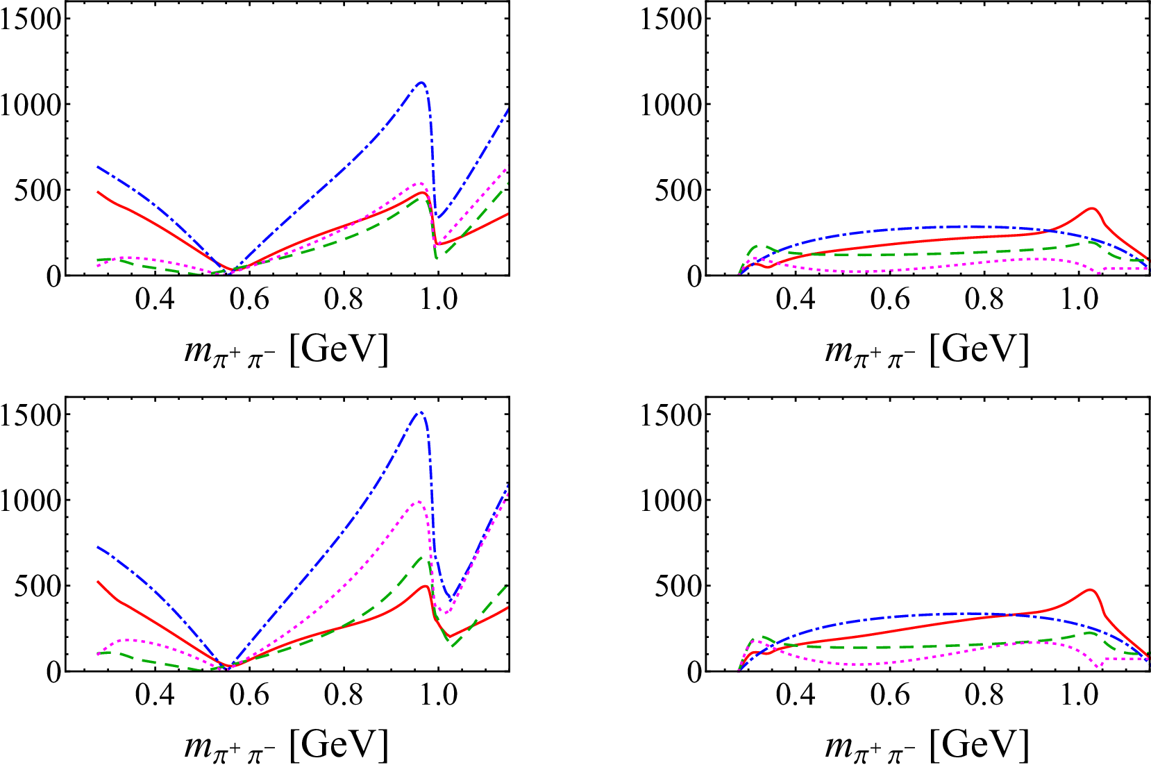
The uncertainty due to the dispersive input for the rescattering is estimated by comparing the fits with the two different matrices (DP Dai:2014lza; Dai:2014zta; Dai:2016ytz vs. BO Leutwyler2012; Moussallam2004). In Fig. 3, the best fit results of the mass spectrum in are shown, where the borders of the bands represent the fit results using these two different matrix parametrizations. The fit results of the ratios of the cross sections are given in Table 1. The fitted parameters as well as the are shown in Tables 2 and 3 for the DP and BO parametrizations, respectively. As can be seen from Fig. 3 as well as Tables 2 and 3, the fit quality to the data set at is worse than that at , in particular in the region close to the lower kinematical boundary and for the highest data point. Notice that by using the inputs from known scattering observables in the dispersion relations, the effects of resonances in the considered partial waves, i.e. the , , and , are included automatically. Since the dataset at has a larger phase space to reveal the nontrivial structure and the fits are better, we discuss the fit results of this data set in more details.

It is interesting to compare Fits IIa and IIb. In Fit IIa, the SU(3) octet chiral contact terms are not included. The experimental data, especially the broad peak in the region lower than , cannot be described well. In contrast, in Fit IIb, including the SU(3) octet chiral contact terms, the fit quality is improved significantly. A similar improvement is also observed comparing Fits Ib and Ia. We also perform two further Fits IIc and IId for the dataset, considering only the contact terms and switching off the left-hand cuts: in Fit IIc we only retain the SU(3) singlet component, while in Fit IId, both the SU(3) singlet and octet components are taken into account. The result is shown in Fig. 4, and the fit couplings are also listed in Table 2. Comparing Fits IIc and IId, one also finds that adding the SU(3) octet component increases the fit quality significantly.
It is instructive to analyze the ratio of the parameters for the SU(3) octet component relative to those for the SU(3) singlet component. Using the results of Fit IIb as shown in Tables 2 and 3, we have and in the DP parametrization and and in the BO one, which agree well with each other within errors. Note that is not as stable as : the reason is that is small in most fits. In the hadronic molecule scenario of , one has
| (42) |
from which the light-quark component reads , where the definitions of the singlet and octet components and have been given below Eq. (1). They thus give the ratio of . Certainly our results (values of ) differ significantly from the result of the pure hadronic molecule scenario. In addition to the hadronic molecule, the may contain other SU(3) singlet sources, e.g., from or a hybrid. Assuming in the transition the strengths of the light-quark components from the hadronic molecule and the other SU(3) singlet source are and , respectively, namely,66 6 Notice that any isoscalar pair of nonstrange charm and anticharm mesons has the same SU(3) structure.
| (43) |
we can estimate the ratio of based on our results of . Thus we conclude that there is a large light-quark SU(3) octet component in the , and scenarios of a hybrid or conventional charmonium are disfavored since the light quarks have to be produced in the SU(3) singlet state in such states. Also our study shows that the component of the may not be completely dominant. This is not unnatural, as the mass, being around , is about below the threshold.
In Fig. 5, we plot the moduli of the - and -wave amplitudes from the chiral contact terms, the -exchange terms, and the triangle diagrams for Fit IIb. An interesting feature is that the -wave contribution is comparable to the -wave contribution in almost the whole phase space. Such a large -wave contribution in the transition again indicates that the cannot be a conventional charmonium state, for which the -wave should be dominant. Notice that in the hadronic molecule interpretation Cleven:2013mka; Lu:2017yhl, the -wave emerges naturally since the decays dominantly into -wave . Also one observes that the contributions from the chiral contact terms and the l.h.c. contributions are of the same order. Amongst the l.h.c. contributions, both the term and the triangle diagrams appear far from negligible. A better distinction of the effects of the and the open-charm loops requires a detailed analysis of the distribution and is beyond the scope of the present paper.
IV Conclusions
We have used dispersion theory to study the processes . In particular, we have analyzed the roles of the light-quark SU(3) singlet state and SU(3) octet state in these transitions. The strong FSI, especially the coupled-channel ( and ) FSI in the -wave, has been considered in a model-independent way, and the leading chiral amplitude acts as the subtraction function in the modified Omnès solution. Through fitting to the data of the invariant mass spectra of and the ratios of the cross sections , we find that the light-quark SU(3) octet state plays a significant role in the transition, which indicates that the contains a large light-quark component. Thus we conclude that the is in all likelihood neither a hybrid nor a conventional charmonium state. Furthermore, through an analysis of the ratio of the light-quark SU(3) octet and singlet components, we show that the does not behave like a pure hadronic molecule. We also find that there is a large -wave component in the invariant spectrum of the . We close this manuscript by anticipating a combined analysis of both the and data. Such an analysis is a necessary step toward revealing the nature of both states, as there is evidence that the events in the are only produced when the latter is constrained in the region Abazov:2018cyu.
Acknowledgments
We acknowledge Rong-Gang Ping for helpful discussions on the experimental analyses and for kindly providing us with the efficiency-corrected data, and Christoph Hanhart for a careful reading of the manuscript and valuable comments and suggestions. This work is supported in part by the Fundamental Research Funds for the Central Universities under Grants No. 531107051122 and No. 06500077, by the National Natural Science Foundation of China (NSFC) under Grants No. 11805059, No. 11747601, and No. 11835015, by NSFC and Deutsche Forschungsgemeinschaft (DFG) through funds provided to the Sino–German Collaborative Research Center “Symmetries and the Emergence of Structure in QCD” (NSFC Grant No. 11621131001, DFG Grant No. TRR110), by the Thousand Talents Plan for Young Professionals, by the CAS Key Research Program of Frontier Sciences (Grant No. QYZDB-SSW-SYS013), by the CAS Key Research Program (Grant No. XDPB09), and by the CAS Center for Excellence in Particle Physics (CCEPP).
References
- (1) B. Aubert et al. (BABAR Collaboration), Phys. Rev. Lett. 95, 142001 (2005).
- (2) S. Godfrey and N. Isgur, Phys. Rev. D 32, 189 (1985).
- (3) G. Pakhlova et al. (Belle Collaboration), Phys. Rev. D 80, 091101 (2009).
- (4) H.-X. Chen, W. Chen, X. Liu, and S.-L. Zhu, Phys. Rep. 639, 1 (2016).
- (5) A. Hosaka, T. Iijima, K. Miyabayashi, Y. Sakai, and S. Yasui, Prog. Theor. Exp. Phys. 2016, 062C01 (2016).
- (6) R. F. Lebed, R. E. Mitchell, and E. S. Swanson, Prog. Part. Nucl. Phys. 93, 143 (2017).
- (7) A. Esposito, A. Pilloni, and A. D. Polosa, Phys. Rep. 668, 1 (2016).
- (8) F.-K. Guo, C. Hanhart, U.-G. Meißner, Q. Wang, Q. Zhao, and B.-S. Zou, Rev. Mod. Phys. 90, 015004 (2018).
- (9) A. Ali, J. S. Lange, and S. Stone, Prog. Part. Nucl. Phys. 97, 123 (2017).
- (10) S. L. Olsen, T. Skwarnicki, and D. Zieminska, Rev. Mod. Phys. 90, 015003 (2018).
- (11) M. Karliner, J. L. Rosner, and T. Skwarnicki, Ann. Rev. Nucl. Part. Sci. 68, 17 (2018).
- (12) C.-Z. Yuan, Int. J. Mod. Phys. A 33, 1830018 (2018).
- (13) E. Kou et al., arXiv:1808.10567.
- (14) A. Cerri et al., arXiv:1812.07638.
- (15) S.-L. Zhu, Phys. Lett. B 625, 212 (2005).
- (16) F. E. Close and P. R. Page, Phys. Lett. B 628, 215 (2005).
- (17) Y. S. Kalashnikova and A. V. Nefediev, Phys. Rev. D 77, 054025 (2008).
- (18) F. J. Llanes-Estrada, Phys. Rev. D 72, 031503 (2005).
- (19) B.-Q. Li and K.-T. Chao, Phys. Rev. D 79, 094004 (2009).
- (20) M. Shah, A. Parmar, and P. C. Vinodkumar, Phys. Rev. D 86, 034015 (2012).
- (21) C.-F. Qiao, Phys. Lett. B 639, 263 (2006).
- (22) S. Dubynskiy and M. B. Voloshin, Phys. Lett. B 666, 344 (2008).
- (23) X. Li and M. B. Voloshin, Mod. Phys. Lett. A 29, 1450060 (2014).
- (24) L. Maiani, V. Riquer, F. Piccinini, and A. D. Polosa, Phys. Rev. D 72, 031502 (2005).
- (25) A. Ali, L. Maiani, A. V. Borisov, I. Ahmed, M. Jamil Aslam, A. Y. Parkhomenko, A. D. Polosa and A. Rehman, Eur. Phys. J. C 78, 29 (2018).
- (26) Z.-G. Wang, Eur. Phys. J. C 78, 933 (2018).
- (27) G.-J. Ding, Phys. Rev. D 79, 014001 (2009).
- (28) Q. Wang, C. Hanhart, and Q. Zhao, Phys. Rev. Lett. 111, 132003 (2013).
- (29) G. Li and X.-H. Liu, Phys. Rev. D 88, 094008 (2013).
- (30) M. Cleven, Q. Wang, F.-K. Guo, C. Hanhart, U.-G. Meißner, and Q. Zhao, Phys. Rev. D 90, 074039 (2014).
- (31) L.-Y. Dai, M. Shi, G.-Y. Tang, and H.-Q. Zheng, Phys. Rev. D 92, 014020 (2015).
- (32) D.-Y. Chen, J. He, and X. Liu, Phys. Rev. D 83, 054021 (2011).
- (33) D. Y. Chen, X. Liu, and T. Matsuki, Eur. Phys. J. C 78, 136 (2018).
- (34) M. Ablikim et al. (BESIII Collaboration), Phys. Rev. Lett. 118, 092001 (2017).
- (35) M. Ablikim et al. (BESIII Collaboration), Phys. Rev. Lett. 118, 092002 (2017).
- (36) M. Ablikim et al. (BESIII Collaboration), Phys. Rev. D 93, 011102 (2016).
- (37) M. Ablikim et al. (BESIII Collaboration), Phys. Rev. Lett. 112, 092001 (2014).
- (38) M. Ablikim et al. (BESIII Collaboration), Phys. Rev. D 96, 032004 (2017); Phys. Rev. D 99, 019903(E) (2019).
- (39) M. Ablikim et al. (BESIII Collaboration), Phys. Rev. Lett. 122, 102002 (2019).
- (40) W. Qin, S.-R. Xue, and Q. Zhao, Phys. Rev. D 94, 054035 (2016).
- (41) Q. Wang, C. Hanhart, and Q. Zhao, Phys. Lett. B 725, 106 (2013).
- (42) M. Albaladejo, F.-K. Guo, C. Hidalgo-Duque, and J. Nieves, Phys. Lett. B 755, 337 (2016).
- (43) T. Mannel and R. Urech, Z. Phys. C 73, 541 (1997).
- (44) Y.-H. Chen, J. T. Daub, F.-K. Guo, B. Kubis, U.-G. Meißner, and B.-S. Zou, Phys. Rev. D 93, 034030 (2016).
- (45) Y.-H. Chen, M. Cleven, J. T. Daub, F.-K. Guo, C. Hanhart, B. Kubis, U.-G. Meißner, and B.-S. Zou, Phys. Rev. D 95, 034022 (2017).
- (46) C. P. Shen et al. (Belle Collaboration), Phys. Rev. D 89, 072015 (2014).
- (47) M. Cleven, F.-K. Guo, C. Hanhart, and U.-G. Meißner, Eur. Phys. J. A 47, 120 (2011).
- (48) P. Colangelo, F. De Fazio, and R. Ferrandes, Phys. Lett. B 634, 235 (2006).
- (49) F.-K. Guo, C. Hanhart, U.-G. Meißner, Q. Wang, and Q. Zhao, Phys. Lett. B 725, 127 (2013).
- (50) T. Mehen and J. W. Powell, Phys. Rev. D 88, 034017 (2013).
- (51) S. Fleming and T. Mehen, Phys. Rev. D 78, 094019 (2008).
- (52) B. Moussallam, Eur. Phys. J. C 73, 2539 (2013).
- (53) C. Schmid, Phys. Rev. 154, 1363 (1967).
- (54) C. Hanhart, Y. S. Kalashnikova, P. Matuschek, R. V. Mizuk, A. V. Nefediev, and Q. Wang, Phys. Rev. Lett. 115, 202001 (2015).
- (55) F.-K. Guo, C. Hanhart, Y. S. Kalashnikova, P. Matuschek, R. V. Mizuk, A. V. Nefediev, Q. Wang, and J.-L. Wynen, Phys. Rev. D 93, 074031 (2016).
- (56) A. Pilloni et al. (JPAC Collaboration), Phys. Lett. B 772, 200 (2017).
- (57) G. Barton and C. Kacser, Nuovo Cimento 21, 593 (1961).
- (58) J. B. Bronzan and C. Kacser, Phys. Rev. 132, 2703 (1963).
- (59) J. Kambor, C. Wiesendanger, and D. Wyler, Nucl. Phys. B465, 215 (1996).
- (60) R. García-Martín and B. Moussallam, Eur. Phys. J. C 70, 155 (2010).
- (61) B. Kubis and J. Plenter, Eur. Phys. J. C 75, 283 (2015).
- (62) Z.-H. Guo and J. A. Oller, Phys. Rev. D 84, 034005 (2011).
- (63) X.-W. Kang, B. Kubis, C. Hanhart, and U.-G. Meißner, Phys. Rev. D 89, 053015 (2014).
- (64) L.-Y. Dai and M. R. Pennington, Phys. Lett. B 736, 11 (2014).
- (65) L.-Y. Dai and M. R. Pennington, Phys. Rev. D 90, 036004 (2014).
- (66) L.-Y. Dai and M. R. Pennington, Phys. Rev. D 94, 116021 (2016).
- (67) I. Caprini, G. Colangelo, and H. Leutwyler, Eur. Phys. J. C 72, 1860 (2012).
- (68) P. Büttiker, S. Descotes-Genon, and B. Moussallam, Eur. Phys. J. C 33, 409 (2004).
- (69) M. Tanabashi et al. [Particle Data Group], Phys. Rev. D 98, 030001 (2018).
- (70) S. Ropertz, C. Hanhart, and B. Kubis, Eur. Phys. J. C 78, 1000 (2018).
- (71) B. Moussallam, Eur. Phys. J. C 14, 111 (2000).
- (72) J. F. Donoghue, J. Gasser, and H. Leutwyler, Nucl. Phys. B343, 341 (1990).
- (73) M. Hoferichter, C. Ditsche, B. Kubis, and U.-G. Meißner, J. High Energy Phys. 06 (2012) 063.
- (74) J. T. Daub, C. Hanhart, and B. Kubis, J. High Energy Phys. 02 (2016) 009.
- (75) K. M. Watson, Phys. Rev. 88, 1163 (1952).
- (76) K. M. Watson, Phys. Rev. 95, 228 (1954).
- (77) A. V. Anisovich and H. Leutwyler, Phys. Lett. B 375, 335 (1996).
- (78) R. Omnès, Nuovo Cimento 8, 316 (1958).
- (79) R. García-Martín, R. Kamiński, J. R. Peláez, J. Ruiz de Elvira, and F. J. Ynduráin, Phys. Rev. D 83, 074004 (2011).
- (80) J. T. Daub, H. K. Dreiner, C. Hanhart, B. Kubis, and U.-G. Meißner, J. High Energy Phys. 01 (2013) 179.
- (81) M. Ablikim et al. (BESIII Collaboration), Phys. Rev. Lett. 119, 072001 (2017).
- (82) M. Ablikim et al. (BESIII Collaboration), Phys. Rev. D 97, 071101 (2018).
- (83) Y. Lu, M. N. Anwar, and B.-S. Zou, Phys. Rev. D 96, 114022 (2017).
- (84) V. M. Abazov et al. (D0 Collaboration), Phys. Rev. D 98, 052010 (2018).