The 2L1S/1L2S Degeneracy for Two Microlensing Planet Candidates Discovered by the KMTNet Survey in 2017
Abstract
We report two microlensing planet candidates discovered by the KMTNet survey in . However, both events have the 2L1S/1L2S degeneracy, which is an obstacle to claiming the discovery of the planets with certainty unless the degeneracy can be resolved. For KMT-2017-BLG-0962, the degeneracy cannot be resolved. If the 2L1S solution is correct, KMT-2017-BLG-0962 might be produced by a super Jupiter-mass planet orbiting a mid-M dwarf host star. For KMT-2017-BLG-1119, the light curve modeling favors the 2L1S solution but higher-resolution observations of the baseline object tend to support the 1L2S interpretation rather than the planetary interpretation. This degeneracy might be resolved by a future measurement of the lens-source relative proper motion. This study shows the problem of resolving 2L1S/1L2S degeneracy exists over a much wider range of conditions than those considered by the theoretical study of Gaudi 1998.
Subject headings
gravitational lensing: micro – exoplanetsI. Introduction
The basic requirements for the statistical studies of planets are detections of planets and the determination of planet properties. However, discoveries and characterizations of microlensing planets depend on the interpretation of anomalies in the observed light curves. Even when these anomalies can be described by a planetary model, there may exist alternative interpretations that also provide sufficient descriptions for the putative planetary anomalies. In other words, degenerate solutions of the light curves can be obstacles to prevent either secure discoveries of planets or the unique determination of their properties.
For example, the degeneracy between two interpretations of the binary-lens and single-source (2L1S) and the single-lens and binary-source (1L2S) can be a severe obstacle. If this 2L1S/1L2S degeneracy exists, we cannot claim a secure discovery of the planet unless the degeneracy is resolved. Gaudi 1998 first pointed out this 2L1S/1L2S degeneracy by showing that a certain class of 1L2S model can resemble a planetary anomaly in the lensing light curve. In particular, he focused on planetary events that exhibit small, short-duration positive deviations from a single-lens, single-source (1L1S) light curve. To produce a similar anomaly in the light curve using a 1L2S model, the brightness of the companion should be much fainter than the primary (the flux ratio of the secondary and primary, , should be from to ). In addition, the companion should pass very close (in projection) to the lens (this impact factor for the secondary, , depends on the maximum amplitude, , of the planet-like anomaly with the flux ratio: ).
Indeed, there are discoveries of microlensing planet candidates, which could be interpreted by both 2L1S and 1L2S models. Beaulieu et al. 2006 found a clear planetary deviation (i.e., a small, short-duration positive deviation) in a microlensing event, OGLE-2005-BLG-390. They also found the 2L1S/1L2S degeneracy that plausibly described the anomaly. However, the 1L2S interpretation was rejected by the detailed light curve analysis. Thus, they could claim the secure discovery of a planet, whose mass they estimated to be . Hwang et al. 2013 also showed a microlensing event that had the 2L1S/1L2S degeneracy. The light curve of this work exhibits a planet-like anomaly (i.e., the strong positive deviation) that can be explained by either the 2L1S (including a planet) or 1L2S interpretations. They successfully resolved this degeneracy using multi-band observations revealing that the event was produced by two sources, rather than a planetary system. In addition, Dominik et al. 2019 recently presented a long timescale ( days) microlensing event, which can be explained either 2L1S or 1L2S interpretations. Their 2L1S model indicates that the lens system might be a planet with the mass orbiting an M-dwarf host star (). However, they also find a competitive 1L2S model that indicates that the lens might be a brown-dwarf (). The light curve data cannot resolve this degeneracy, but they suggest future observations may be able to resolve this severe degeneracy.
However, in practice, we have found that the 2L1S/1L2S degeneracy can be extended to cases beyond the extreme flux case considered by Gaudi 1998, e.g., Jung et al. 2017a, Dominik et al. 2019, and events in this work. In Jung et al. 2017a, the light curve of the event showed a broad asymmetry with small additional deviations in the wing. This anomaly can be adequately described by both the 2L1S (i.e., a planetary lens system) and the 1L2S interpretations. This event was produced by close to equal-luminous binary sources in contrast to the case of Gaudi 1998. They resolved this degeneracy using detailed modeling of the densely covered light curve. In Dominik et al. 2019, they showed that the planet-like anomaly in the 2L1S case could be produced when the source passes close to the central caustic, i.e., a high-magnification event. This anomaly is different from Gaudi’s case, which is produced when the source approaches one of planetary caustics. They noted that the 1L2S model with a small flux ratio of binary sources can produce this planet-like anomaly in contrast to Gaudi’s case.
In addition, microlensing events showing more complex anomalies have been found. These events can be described by more complicated multiple-lens and multiple-source interpretations. For example, Jung et al. 2017b showed a degeneracy caused by 3L1S and 2L2S interpretations. Moreover, Hwang et al. 2018 showed an extreme case (i.e., exo-moon candidate) of a three-fold degeneracy with 3L1S, 2L2S, and 1L3S interpretations. In particular, the degeneracy becomes severe when the observations do not optimally cover the anomalies in the light curves.
Here we analyze two microlensing events, KMT-2017-BLG-0962 and KMT-2017-BLG-1119, that were discovered in by the Korea Microlensing Telescope Network (Kim et al. 2016, KMTNet:). We reveal that these events are planet candidates by analyzing the light curves using the 2L1S interpretation. For KMT-2017-BLG-0962, the mass ratio () is , which indicates that the companion in the lens system might be a Jupiter-class planet under the assumption of an M-dwarf host star. For KMT-2017-BLG-1119, the mass ratio is , which also indicates that the lens component might be a planet. Moreover, the Einstein timescale () of this event is very short, i.e., days. This short timescale implies that the event can be produced by a very low-mass planetary lens system11 1 The Einstein timescale is a crossing time that the source transverses the Einstein ring radius (), i.e., . The size of is directly related to the mass of the lens system (), i.e., where . and are distances to the lens and source, respectively. Thus, , which are of order a month for typical microlensing events.. However, both light curves can also be well described using the 1L2S interpretation.
We present observations of these planet candidates in Section 2. In Section 3, we present analyses of the light curves and the degeneracies. Then, we discuss the possibilities of resolving the degeneracies in Section 4. In Section 5, we present the possible properties of planet candidates determined using the Bayesian analyses. Lastly, in Section 6, we present our conclusion with the difference between a Gaudi 1998-type degeneracy and this work. Additionally, we provide details of the 1L2S interpretations for the modeling in Appendix A. We also present tests for higher-order effects of the models to discuss non-detections of them in Appendix B.
II. KMTNet Observations
KMTNet is a second-generation microlensing survey consisting of a telescope network composed of three identical m telescopes located at three sites in the southern hemisphere: the Cerro Tololo Inter-American Observatory in Chile (KMTC), the South African Astronomical Observatory in South Africa (KMTS), and the Siding Spring Observatory in Australia (KMTA). These well-separated time zones can provide near-continuous observations, weather permitting. In addition, the cameras of the KMTNet survey have a wide field of view (FOV: ). These wide FOV yield high-cadence observations that are optimized to capture planetary anomalies caused by various types of planets. Thus, in general, the KMTNet survey (i.e., a second-generation microlensing survey) is less dependent on follow-up observations.
KMTNet discovered the two planet candidates presented in this work. The events were found by the KMTNet Event Finder algorithm (Kim et al. 2018), which was run after the end of the microlensing season. No real-time alert was issued for these events, either by KMTNet or other microlensing groups. Hence, no useful real-time photometric follow-up observations were taken22 2 KMT-2017-BLG-1119 was in fact serendipitously observed by the Spitzer satellite because it lies within the IRAC camera field of view of another event (OGLE-2017-BLG-0019) that was chosen for observations (see Yee et al. 2015). Unfortunately, these observations ended (due to sun-angle restrictions) on , just two days before the peak of this very short event. In principle, if the lens were traveling approximately east, the source could nevertheless have been significantly magnified. However, we have checked the images and found that the Spitzer light curve of KMT-2017-BLG-1119 is essentially flat. Thus, no meaningful constraints can be placed on this system from the Spitzer data..

However, we found that KMT-2017-BLG-1119 was located within the footprint of another survey. The Microlensing Observations in Astrophysics (Sumi et al. 2003, MOA:) survey observed this event using the m MOA-II telescope located at the Mount John Observatory in New Zealand, with the customized filter called MOA-Red filter (wide filter). Because the MOA survey did not alert this event during the season, we separately requested the MOA data of the event. The data were reduced using their pipeline employed the difference image analysis (DIA) photometry (Bond et al. 2001). In contrast, KMT-2017-BLG-0962 is not located in the MOA observation fields.

II.1. KMT-2017-BLG-0962
KMT-2017-BLG-0962 occurred on source(s) located at corresponding to the Galactic coordinates . This event is located in the KMT-field, BLG18 (see Figure 12 of Kim et al. 2018), which has the nominal observational cadence . During the event, the cadence was at KMTC. For the other observations, the cadence was . In Figure 1, we present KMTNet observations of this event with a 1L1S model curve as a reference to clearly show the anomaly in the light curve. There exist clear perturbations around the peak of the event, .
II.2. KMT-2017-BLG-1119
KMT-2017-BLG-1119 occurred on source(s) located at corresponding to the Galactic coordinates . This event is located in the KMT-field, BLG22, which also has the nominal cadence . During the event, this was an actual cadence for KMTC observations. For KMTS and KMTA observations, the cadence was switched from to at , i.e., just after the event peaked. In Figure 2, we present the KMTNet and MOA observations of this event. The observations show clear deviations (from to ) from the 1L1S model.
III. Interpretations of the Light curves
Because both events show clear anomalies in the observed light curves, we analyze the light curves using both 2L1S and 1L2S interpretations. For each interpretation, we build model light curves using an appropriate parameterization. Then we minimize the difference between the model and observations by using a Markov Chain Monte Carlo (MCMC) algorithm (Dunkley et al. 2005).
| parameter | 2L1S (close) | 2L1S (wide) | parameter | 1L2S |
|---|---|---|---|---|
| (HJD’) | ||||
| (days) | ||||
Note. — We present upper limits () of the parameters for the 2L1S models. Because this event does not have caustic-crossings, the parameters are not accurately measured (see Figure 5). For the 1L2S models, the finite source effect is not considered for modeling.
During the modeling process, the uncertainties of observations are rescaled using the equation, , where the and are rescaled and original uncertainties in magnitudes, respectively.33footnotetext: In general, the error rescaling is used a quadrature formalism: , where and are error rescaling factors. However, we find that the factors should be zero for observations of both events. Thus, we only present the factor without the meaningless zero terms.
In principle, the factor has an uncertainty of . Neglecting this factor can affect the interpretation of the difference between two models. Specifically, it leads to an uncertainty in the of . Hence, for , so that for example would formally be written (for three observatories). This uncertainty in has no practical impact in the present case, so we suppress it in all expressions. The coefficient , an error rescaling factor for each dataset, is defined based on the best-fit model having the lowest value. By making sure each data point contributes on average , we can quantitatively compare the degenerate models. For KMT-2017-BLG-0962 and KMT-2017-BLG-1119, the sets of error rescaling factors are and , respectively.
III.1. Parameterization of the 2L1S Interpretation
To build a standard 2L1S model light curve, seven basic parameters are required to describe the caustic form and the source trajectory. Two parameters ( and ) determine the caustic form. The value represents the projected separation between the lenses in units of the angular Einstein ring radius (). Conventionally, cases of and are referred to “close” and “wide”, respectively. The mass ratio of the lenses is defined as where and are masses of first and second bodies, respectively. These close and wide cases can yield a close/wide degeneracy caused by similarities in the magnification pattern, which are induced by an intrinsic symmetry in the lens equation (Griest & Safizadeh 1998; Dominik 1999).
Four parameters (, , , and ) describe the source trajectory: is the time when the source most closely approaches to the reference position of the lens system (this reference position is the photo-center (Kim et al. 2009) defined as and for the close () and wide () cases, respectively), is the separation at the time of , is the Einstein timescale defined as the time for the source to cross the Einstein ring radius of the event, and is the angle of the source trajectory with respect to the binary axis of the lens system. The geometry of a microlensing event produced by 2L1S is built using these six parameters, which determine the magnification as a function of time, i.e., the microlensing light curve. The finite angular size of the source moderates the magnification. To account for the finite source effect, the final parameter, , is required, which is defined as the angular source radius () scaled by . In addition, we introduce two additional parameters, (source flux) and (blending flux), for each dataset, which are used to scale the model to the data. These parameters are determined based on the model using the least-square fitting method.
III.2. Parameterization of the 1L2S Interpretation
A standard 1L2S model light curve is built using a superposition of two 1L1S light curves induced by each source. The trajectory of each source yields the individual magnification of its 1L1S light curve. For the 1L2S model light curve, the final magnification is calculated by superposing magnifications of both sources weighted by the flux ratio of source stars. To describe the source trajectories, there are two parameterizations. The first parameterization (hereafter, A-type) describes the trajectory of each source, individually. In contrast, the second parameterization (hereafter, B-type) describes the barycenter motion of the binary-source system. Then, from the position of the barycenter, the position of each source is derived. In Appendix A, we provide detailed descriptions of these parameterizations and discuss the pros and cons of the two types. In this work, because the merits of the two types are different, we adopt the A-type for the basic 1L2S modeling (Section 3.3 and 3.4). For testing the higher-order effects, we adopt the B-type (Section 3.4).
III.3. Degenerate Models
| parameter | 2L1S | parameter | 1L2S |
|---|---|---|---|
| (HJD’) | |||
| (days) | |||
Note. — For the 1L2S models, the finite source effect is not considered for modeling.
III.3.1 KMT-2017-BLG-0962
For KMT-2017-BLG-0962, we find that the observed light curve can be described using either 2L1S and 1L2S interpretations. In Figure 1, we present the observed data and model light curves of this event with geometries of the 2L1S and 1L2S interpretations. We also present residuals between the models and observations. In Table 1, we present the model parameters of best-fit models with between the models and observations. The 2L1S model indicates that this event can be caused by a planetary lens system with a mass ratio between the lens components. However, there is a degeneracy between the close and wide solutions. At the same time, the 1L2S model implies that the event can also be caused by a binary-source system. The planetary model (2L1S models of the close and wide cases) and 1L2S model are completely degenerate. The differences between 1L2S and 2L1S are only and for the close and wide cases, respectively. Thus, we cannot claim a certain planet discovery.
III.3.2 KMT-2017-BLG-1119
For KMT-2017-BLG-1119, we find that the observed light curve is also well-described by both interpretations. In Figure 2, we present light curves of these degenerate models with their geometries and residuals. In Table 2, we present the parameters of these degenerate models. In contrast to the previous case, these models show slight variations. The best-fit model, 2L1S, shows a low mass ratio () with very short Einstein timescale ( days). This indicates that this event can be caused by a low-mass planetary lens system. However, this event also can be well described by the 1L2S interpretation, which implies that the planet would not exist. Quantitatively, the difference between 1L2S and 2L1S is . This value is too marginal to claim the 2L1S/2L1S degeneracy is resolved considering the severe systematics of the observations (see residuals of Figure 2). The cannot be conclusive evidence to resolve the degeneracy (we discuss more details of the difference in Section 4.1).
III.4. Higher-order Effects of the Interpretations
Even though both events have the 2L1S/1L2S degeneracy, it is possible that these events were caused by planetary lens systems. Thus, for the 2L1S interpretation, we check the possibility of measuring the annual microlens parallax (Gould 1992, APRX:) because the microlens parallax is not only a key observable for directly determining the properties of the lens system but also a strong constraint for estimating the properties using the Bayesian analysis. However, we cannot find any meaningful improvements for both events to claim the detection of the APRX signals when we consider the APRX models by introducing the additional parameters of the microlens parallax.
For the 1L2S interpretation, the binary sources orbit each other and conserve their angular momentum. This source-orbital motion can affect the light curve. In addition, the source-orbital effect can be a clue to resolving the 2L1S/1L2S degeneracy. Thus, we test the effect of the source-orbital motion by adopting the B-type parameterization with two additional orbital parameters (see Appendix A for details of this parameterization). However, we cannot find any meaningful signals in the light curves of both events caused by the orbital motion of the sources (for the details of non-detection of these higher-order effects, see Appendix B).
IV. Resolving the Degeneracy
IV.1. Detailed Analysis of the Light curve
We now consider whether the 2L1S/1L2S degeneracy can be resolved in either of the two events. There are several methods that may be employed to resolve this degeneracy, most of which were discussed by Gaudi 1998. The first method is the detailed analysis of the light curve to check for small differences between the two models.
For KMT-2017-BLG-0962, the difference between the 2L1S and 1L2S models is insignificant, and Figure 1 shows that the three models are quite similar. In contrast to the Gaudi 1998 case, there are no caustic-crossings. There exists only a smooth deviation from a 1L1S event. Thus, for this event, the differences in the light curve are not sufficient to resolve the degeneracy.

For KMT-2017-BLG-1119, the best 2L1S model is preferred by over the 1L2S model. However, even though the degeneracy is formally broken, the distinction is not as strong as it appears. In Figure 3, we present plots of the cumulative of each model to investigate the origin of the improvement. We find that the improvement starts at , which is a part of the light curve covered by MOA and KMTC observations. The improvement mostly comes from the MOA observations. Quantitatively, among the total improvement, the MOA and KMTC data contribute and , respectively. However, both datasets have systematics that persist even in the best model (see lower four panels of zoom-in in Figure 3). This fact suggests that a significant portion of the improvement could just be from fitting systematics in the data. Thus, cannot be a conclusive clue to resolve the 2L1S/1L2S degeneracy. In addition, while this still indicates a preference for the 2L1S model, the physical parameters derived from the Bayesian analysis in Section 5.2.2 predict an extreme system in which the host itself is a massive planet. Thus, we should consider other means of testing the models to independently resolve the degeneracy.
IV.2. Color Information of the Source(s)
The second method is to use the source-color information. Because the magnification of the 1L2S model is a weighted mean using the flux ratio of the sources (see Appendix A), the final magnification is wavelength dependent. Thus, if the binary sources have different colors (and the event really is a 1L2S event), we can measure the color change or difference during the perturbation from multi-band observations. However, unfortunately, the signal-to-noise ratio of V-band observations (the KMTNet regularly takes V-band images) for both events is too low to apply this method. Thus, we cannot resolve the degeneracy using this method.
IV.3. Other Methods to Resolve the Degeneracy
Gaudi 1998 also proposed additional observations to resolve the degeneracy if the previous methods fail. One spectroscopic method requires taking spectra of the source both during and after the perturbations of the event. However, this method cannot be used after the events have ended. The other method requires photometrically and spectroscopically monitoring of the source after the event to search for other signals induced by the binary source such as radial velocity variations due to orbital motion or eclipses. Given the faintness of the source(s), spectroscopic monitoring would be challenging. And given the source separations ( and for KMT-2017-BLG-0962 and KMT-2017-BLG-1119, respectively), the probability of eclipses is extremely low. In addition, Calchi Novati et al. 2018 presented a new method to resolve the 2L1S/1L2S degeneracy using simultaneous ground- and space-based observations. However, unfortunately, space-based data do not exist for these events (see footnote 2).
IV.4. Measurement of the Baseline Object
Because most possibilities, which are proposed by other studies, are not helpful to resolve the 2L1S/1L2S degeneracy of our cases, we consider another possibility to resolve the degeneracy using higher-resolution follow-up observations to directly measure the magnitude of the source(s) for these events. For KMT-2017-BLG-1119, we found different source fluxes () for the 2L1S and 1L2S interpretations (see Table 2). If this event was caused by the planetary system, the magnitude of the source will be and the lens is predicted to be dark. If this event was caused by binary sources, the integrated magnitude of the sources will be observed . We note that these expected I magnitudes are calibrated to the OGLE-III magnitude system by cross-matching between KMTNet and OGLE-III catalogs .

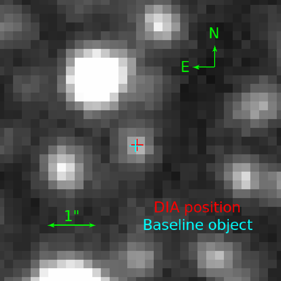
We check the expected brightness of the baseline object using observations taken from the Canada-France-Hawaii Telescope (CFHT) located at the Maunakea Observatories in . In Figure 4, we present the CFHT image with the astrometric offset between the positions of the baseline object obtained from CFHT and KMTNet observations. The offset is . From the CFHT image, we measure the brightness of the baseline object. We also see that the baseline object is close to coincident with the event and isolated. Thus, it is highly likely that the light from the baseline object is composed of light from stars related to the event. Thus, the CFHT measurement can be a constraint to check the degenerate solutions of this event. From the stacked deep CFHT image (seeing), we can measure the brightness of the baseline object: (we note that the CFHT instrumental magnitude is also calibrated to the OGLE-III magnitude system). The measurement of the baseline object is consistent with the expectation of the 1L2S interpretation considering its uncertainty. Therefore, this constraint supports the conclusion that this event might be caused by the 1L2S system. However, we cannot guarantee that the CFHT measurement completely excludes blend light from unrelated stars. Thus, the possibility of the 2L1S origin cannot be clearly ruled out although it is disfavored.

The 2L1S solution predicts a lens-source relative proper motion of . Thus, if a thirty-meter class telescope made observations a decade after the event and the relative proper motion of the source and lens were measured to be significantly different from 2L1S value, that would rule out that solution. On the other hand, if the proper motion were consistent with the 2L1S value, that would tend to support the planetary solution but would not be definitive. Note that such a measurement (as always) requires that the lens (or a companion to the lens) be luminous. However, the short timescale of this event favors low-mass lenses, which might fail this condition.
| event | KMT-2017-BLG-0962 | KMT-2017-BLG-1119 | ||||
|---|---|---|---|---|---|---|
| model | close | wide | resonant | |||
| parameter | ||||||
| 0.706 | 0.593 | 0.672 | 0.597 | 0.766 | 0.780 | |
| 29.780 | 0.007 | 31.103 | 0.006 | 2.826 | 0.030 | |
| 4.745 | 0.004 | 5.452 | 0.004 | 0.105 | 0.003 | |
| 1.683 | -3.077 | 2.022 | -3.164 | 1.285 | 1.201 | |
In contrast, for KMT-2017-BLG-0962, we obtained almost identical values of the (see Table 1). Thus, for this event, the measurement of the baseline object using higher-resolution follow-up observations would not be helpful for resolving the degeneracy.
V. Properties of Planet Candidates
V.1. Bayesian Analyses
Because we cannot measure the microlens parallax, we estimate the properties of these planet candidates using the Bayesian analyses. We build a prior by generating artificial microlensing events (the total number of simulated events is ). To generate these events, we adopt the Galactic models from various studies: initial and present-day mass functions of Chabrier 2003, velocity distributions of Han & Gould 1995, and matter density profiles of the Galactic bulge and disk of Han & Gould 2003. When these artificial microlensing events are generated, the line of sight to the actual event is considered. This prior contains various information about host properties according to the event rate. Based on the event rate, we calculate the posterior probability distributions of the lens properties, by applying constraints obtained from the actual event.

The constraints are built in the form of weight functions, which are obtained from the and distributions of the actual event. In Figures 5 and 6, we present the distributions of selected parameters (, , and ), the first two of which are used to build the weight functions and determine the lens properties for KMT-2017-BLG-0962 and KMT-2017-BLG-1119, respectively. The distributions show a skewed Gaussian form, which we parameterize by,
| (1) |
where the function indicates an error function defined as . The variable is or . The set of (, , , ) are fitting parameters. We use the MCMC algorithm to fit these parameters. The fitting results, i.e., and weight functions, and , are presented in Figures 5 and 6 (cyan lines). In Table 3, we present the best-fit parameter sets of and for both events. The final weight function is . By applying the final weight function to the event rate, we construct probability distributions of the host mass (), the distance to the lens (), the physical Einstein ring radius (), and the lens-source relative proper motion (). From these probability distributions, we can determine the properties of the planet candidate of each event.
V.2. Angular Source Radius
For applying the to the event rate, the angular source radius () is required to convert from (for the artificial lensing events) to (). However, unfortunately, we do not have reliable V-band data to estimate . Thus, we cannot adopt the conventional method (Yoo et al. 2004) using () color of the source for measuring the . For each event, we estimate using different methods because the available observations are different.
V.2.1 KMT-2017-BLG-0962
For this event, reliable observations to measure the source color do not exist. Thus, we adopt a statistical method (Bennett et al. 2008, established in) to estimate the source color using Hubble Space Telescope (HST) observations of Baade’s window (Holtzman et al. 1998).
The source magnitude offset from the red giant clump () is determined from comparing the source flux () obtained from the pyDIA light curve to the red giant clump centroid measured from the color-magnitude diagram (CMD). Then, we extract HST stars having similar magnitude offset to those of the source of the event. Using this extracted HST star sample (and excluding outliers in ), we determine the median star color () and the standard deviation of the color (). Then, we take this HST star color with uncertainty as representative of the source color: . By adopting the clump color for the HST CMD from Bennett et al. 2008, we find the offset of the source from the clump is . Then, using the intrinsic color (Bensby et al. 2011, ) and magnitude (Nataf et al. 2013, ) of the red giant clump along this line of sight, we derive: . Lastly, is estimated using the color/surface-brightness relation adopted from Kervella et al. 2004:
| (2) |
In Figure 7, we present the combined CMDs of events where the centroids of the red giant clumps are aligned to the unextincted red giant clump magnitudes.
| event | KMT-2017-BLG-0962 | KMT-2017-BLG-1119 | |||
|---|---|---|---|---|---|
| constraints | only | ||||
| model | close | wide | close | wide | resonant |
| w/ stellar remnants | |||||
| (kpc) | |||||
| (au) | |||||
| (au) | |||||
| w/o stellar remnants | |||||
| (kpc) | |||||
| (au) | |||||
| (au) | |||||
Note. — For KMT-2017-BLG-1119, the median values with and without stellar remnant hosts are identical. Thus, we present one case to avoid clutter.


V.2.2 KMT-2017-BLG-1119
For this event, MOA R-band observations exist. Thus, we can measure the () color of the source from source fluxes of the model fits of MOA () and KMTNet () light curves: . Then, we cross-match stars between the KMTNet and MOA CMDs with the OGLE-III catalog (Szymański et al. 2011) to derive a relation to convert to . By combining the measured () source color and conversion relation, we can determine the position of the source on the cross-matched CMD (in OGLE-III magnitude scales): . Then, by adopting the method of Yoo et al. 2004 and intrinsic color (Bensby et al. 2011, ) and magnitude (Nataf et al. 2013, ) of the red giant clump, we can measure the de-reddened () source color: . Then, we determine the using the color/surface-brightness relation (Kervella et al. 2004):
| (3) |
In Figure 7, we present the de-reddened KMTNet CMD with positions of the source and centroid of the red giant clump.
V.3. Bayesian Results
V.3.1 KMT-2017-BLG-0962
For KMT-2017-BLG-0962, we expect the constraint (combined with and ) to have only a weak effect on the Bayesian analysis because the constraint of is weak for this event (see Figure 5). In addition, we have had to estimate by estimating the source () using HST observations of Baade’s window rather than making a direct measurement. Thus, we conduct Bayesian analyses with and without the constraint. In addition, the posterior distributions are constructed using Galactic priors with and without stellar remnants as hosts of the lens system because we cannot rule out the possibility of stellar remnant hosts. Thus, for the degenerate 2L1S solutions (i.e., close and wide), we conduct four types of Bayesian analyses. In Figure 8, we present the results of the Bayesian analyses. In Table 4, we present median values of the distributions as representative of the lens system with () confidence intervals. The Bayesian results both with and without the constraint are consistent considering the confidence intervals. The results indicate that this event can be produced by a planetary system consisting of a mid-M dwarf host star and a super Jupiter-mass planet orbiting beyond the snow line.
V.3.2 KMT-2017-BLG-1119
For KMT-2017-BLG-1119, the 2L1S interpretation is disfavored considering the CFHT measurement of the baseline object. Although the 2L1S solution is disfavored, we report the Bayesian results for completeness. In Figure 9, we also present the probability distributions of the lens properties. Because the timescale of this event is particularly short, the distributions with and without stellar remnant hosts show identical results. Thus, we present one case. In Table 4, we also present median values of the distributions.
The Bayesian results suggest that the lens system of this event may be interesting. If the 2L1S solution is correct, the lens system is most likely to be a sub-Saturn-mass planet with a mass () orbiting a brown dwarf host with a mass . Indeed, these kinds of planetary systems having faint/dark hosts () were discovered by the microlensing method (Bennett et al. 2008; Han et al. 2013; Sumi et al. 2016; Shvartzvald et al. 2017; Jung et al. 2018a; Jung et al. 2018b; Miyazaki et al. 2018, e.g.,). Microlensing is one useful method to search these kinds of systems because the method can discover planets regardless of the brightness of the hosts. However, we note that the 2L1S interpretation for this event is disfavored. Thus, it is unclear whether or not this event contains an example of such a planetary system.
VI. Conclusion
We have presented the analysis of two microlensing events with candidate planets. From Bayesian analysis, we determine the properties of the planet candidates. For KMT-2017-BLG-0962, the lens system may consist of a super Jupiter-mass planet and a mid-M dwarf host. However, the severe 2L1S/1L2S degeneracy of this event, which is unresolvable, prevents claiming this planet discovery with certainty. For KMT-2017-BLG-1119, the 2L1S interpretation would indicate that the lens system consists of a sub-Saturn-mass planet and a brown dwarf host. However, the CFHT imaging supports the 1L2S interpretation rather than this potential interesting planetary system. The planetary solution could be tested with the possibility of conclusively ruling it out by a future measurement of the lens-source relative proper motion.
The 2L1S/1L2S degeneracies described in this work (and also the degeneracy in Jung et al. 2017a) are far different from the degeneracy for small, short-duration positive anomalies shown in Gaudi 1998. The anomalies are of much longer duration and affect a significant fraction of the light curves, yet the degeneracy remains. In addition, the magnitude difference () between the two sources is not very extreme () in contrast to Gaudi’s case. These events are similar to the event recently analyzed in Dominik et al. 2019. These cases show that the 2L1S/1L2S degeneracy can exist for a wide range of planetary events and for much less extreme binary source systems. Because binary stars are common and this degeneracy has proven not to be limited to a rare subset of binaries, the 2L1S/1L2S degeneracy may be a bigger problem for the discovery of planets than previously thought.
Appendix A Two Parameterizations of the 1L2S Interpretation

In Figure 10, we present conceptual geometries of the 1L2S interpretation for two types of parameterizations. The A-type parameterization (see the left panel of Figure 10) requires six parameters: , , , , , and (Griest & Hu 1992). The first five parameters are directly related to the source trajectories: and are the time when each source most closely approaches the reference position (i.e., the position of the lens), and represent the closest separation between each source and the reference position at the time of and , respectively, is the Einstein timescale. We use one parameter assuming that the lens-source relative speeds are same for both sources, i.e., a comoving binary-source system. The last parameter, is the flux ratio of the sources. The role of is to weight the two 1L1S light curves produced by the individual sources.
By adopting this parameterization, the position of each source as a function of time () is defined in Cartesian coordinates normalized by as
| (A1) |
According to the positions of the sources, the magnification of each source, , is defined as
| (A2) |
These magnifications are superposed by weighting by the ratio of source fluxes, . Then, the final magnification of the lensing light curve, , is calculated as
| (A3) |
This model light curve in the magnification scale is converted to the flux scale of each dataset for comparison to the observations using two additional parameters, and (similar to those of the 2L1S interpretation). These additional parameters are determined using the least-square fitting method.
The merit of this A-type parameterization is that it is possible to directly guess the initial values of most parameters (except ) from the observed light curve. However, the A-type parameterization has a disadvantage that it is difficult to apply higher-order effects, especially the orbital motion of the binary-source system.
Thus, we introduce an alternative parameterization, B-type (see right panel of Figure 10), which considers the motion of the barycenter of the binary-source system (Jung et al. 2017a), rather than the motion of each source. To describe the barycenter motion, it requires three parameters (, , ): is the time when the barycenter closely approaches to the reference position, is the closest separation at the time of , and is the Einstein timescale. To derive the trajectory of each source from the barycenter trajectory, three additional parameters (, , ) are required to describe the binary-source system: is the projected separation between the sources, is a mass ratio of the source stars, and is an angle between the axis of the binary-source and the barycenter trajectory. In addition, there is the last parameter () that is identical to that of the A-type parameterization.
By adopting this parameterization, the source positions are defined as
| (A4) |
where the and are the separations between the barycenter and each source, which are defined as
| (A5) |
Based on the positions of the source, the final model light curve is constructed in the same way as the previous parameterization (see Equations A2 and A3).
This B-type parameterization has merit when higher-order effects are considered. In particular, the orbital motion of the binary-source can be easily introduced because the binary source positions are defined from the barycenter. To introduce the source-orbital motion, two additional parameters, and , are required. These parameters are the variation rates of and to describe a partial orbit of the binary-source system. The variations are derived as
| (A6) |
where is a reference time for describing the orbital motion of sources (we set for the modeling in this work). Thus, the source trajectories are varied by the source-orbital motion, which are described by modifying Equations A4 and A5 as,
| (A7) |
However, the downside of this B-type parameterization is that it is particularly difficult to guess the initial parameters for describing the binary-source system (i.e., , , and ). Thus, usually, this parameterization is only adopted for testing higher-order effects.
Appendix B Non-detections of Higher-order Effects
B.1. The Annual Microlens Parallax (APRX) Effect of the 2L1S Interpretation

The APRX is caused by the orbital motion of Earth (Gould 1992). Thus, the Einstein timescale () is a direct indicator for estimating the possibility of detecting the APRX signal. Empirically, to detect the APRX signal, the event should last more than days. For KMT-2017-BLG-0962, is about days, which implies that there is a chance to detect the APRX signal in the light curve. Thus, we try to measure the APRX by introducing two additional parameters, and , which indicate the north and east directions of the microlens parallax vector (), respectively. From the model considering the APRX, we find improvements, and , for the close and wide cases, respectively. However, these improvements originate in fits of systematics in the baseline, which are caused by accidental caustic-crossing and approach (See Figure 11). This fact implies that the APRX is not significantly constrained in these fits. Thus, we cannot extract any useful information from the APRX model for this event. For KMT-2017-BLG-1119, is only days, which means that it is unlikely to exist the APRX signal can be detected in the light curve. However, for consistency, we also test the APRX model for this event. From the model, as expected, the APRX signal is not detected.
B.2. The Source-orbital Effect of the 1L2S Interpretation

For the 1L2S interpretation, the binary sources always orbit each other to conserve their angular momentum. As a result, this source-orbital motion can affect the light curve if the microlensing event was caused by the 1L2S. It implies that once we may find the source-orbital effect on the lensing light curve, we can obtain a key clue to resolve the 2L1S/1L2S degeneracy. Therefore, we test the effect by introducing additional parameters of the simplified source-orbital motion (see Appendix A, B-type parameterization). The possibility of the detection of the source-orbital effect depends on the timescale of the event, similar to the APRX effect. As expected, for KMT-2017-BLG-1119, there is no improvement considering the very short of this event. In contrast, for KMT-2017-BLG-0962, we find a small improvement () when the source-orbital effect is considered. We investigate this improvement using the cumulative difference plot. See Figure 12. From the investigation, we find that the improvement mostly comes from the fitting of the “bump-like” feature in the baseline (). It is unclear whether this feature is real or due to some systematics in the baseline of the event. With for additional degree of freedom, the significance is too low to claim a detection.
References
- Beaulieu et al. (2006) Beaulieu, J.-P., Bennett, D. P., Fouqué, P., et al. 2006, Nature, 439, 437
- Bennett et al. (2008) Bennett, D. P., Bond, I. A., Udalski, A., et al. 2008, ApJ, 684, 663
- Bensby et al. (2011) Bensby, T., Adén, D., Meléndez, J., et al. 2011, A&A, 533, A134
- Bond et al. (2001) Bond, I. A., Abe, F., Dodd, R. J., et al. 2001, MNRAS, 327, 868
- Calchi Novati et al. (2018) Calchi Novati, S., Skowron, J., Jung, Y. K., et al. 2018, AJ, 155, 261
- Chabrier (2003) Chabrier, G. 2003, PASP, 115, 763
- Dominik (1999) Dominik, M. 1999, A&A, 349, 108
- Dominik et al. (2019) Dominik, M., Bachelet, E., Bozza, V., et al. 2019, MNRAS, 484, 5608
- Dunkley et al. (2005) Dunkley, J., Bucher, M., Ferreira, P. G., et al. 2005, MNRAS, 356, 925
- Gaudi (1998) Gaudi, B. S. 1998, ApJ, 506, 533
- Griest & Safizadeh (1998) Griest, K., & Safizadeh, N. 1998, ApJ, 500, 37
- Griest & Hu (1992) Griest, K., & Hu, W. 1992, ApJ, 397, 362
- Gonzalez et al. (2012) Gonzalez, O. A., Rejkuba, M., Zoccali, M., et al. 2012, A&A, 543, A13
- Gould (1992) Gould, A. 1992, ApJ, 392, 442
- Han & Gould (1995) Han, C., & Gould, A. 1995, ApJ, 447, 53
- Han & Gould (2003) Han, C., & Gould, A. 2003, ApJ, 592, 172
- Han et al. (2013) Han, C., Jung, Y. K., Udalski, A., et al. 2013, ApJ, 778, 38
- Holtzman et al. (1998) Holtzman, J. A., Watson, A. M., Baum, W. A., et al. 1998, AJ, 115, 1946
- Hwang et al. (2013) Hwang, K.-H., Choi, J.-Y., Bond, I. A., et al. 2013, ApJ, 778, 55
- Hwang et al. (2018) Hwang, K.-H., Udalski, A., Bond, I. A., et al. 2018, AJ, 155, 259
- Jung et al. (2017a) Jung, Y. K., Udalski, A., Yee, J. C., et al. 2017a, AJ, 153, 129
- Jung et al. (2017b) Jung, Y. K., Udalski, A., Bond, I. A., et al. 2017b, ApJ, 841, 75
- Jung et al. (2018a) Jung, Y. K., Udalski, A., Gould, A., et al. 2018, AJ, 155, 219
- Jung et al. (2018b) Jung, Y. K., Hwang, K.-H., Ryu, Y.-H., et al. 2018, AJ, 156, 208
- Kervella et al. (2004) Kervella, P., Thévenin, F., Di Folco, E., et al. 2004, A&A, 426, 297
- Kim et al. (2009) Kim, D., Han, C., & Park, B.-G. 2009, JKAS, 42, 39
- Kim et al. (2016) Kim, S.-L., Lee, C.-U., Park, B.-G., et al. 2016, JKAS, 49, 37
- Kim et al. (2018) Kim, D.-J., Kim, H.-W., Hwang, K.-H., et al. 2018, AJ, 155, 76
- Miyazaki et al. (2018) Miyazaki, S., Sumi, T., Bennett, D. P., et al. 2018, AJ, 156, 136
- Nataf et al. (2013) Nataf, D. M., Gould, A., Fouqué, P., et al. 2013, ApJ, 769, 88
- Shvartzvald et al. (2017) Shvartzvald, Y., Yee, J. C., Calchi Novati, S., et al. 2017, ApJ, 840, L3
- Sumi et al. (2003) Sumi, T., Abe, F., Bond, I. A., et al. 2003, ApJ, 591, 204
- Sumi et al. (2016) Sumi, T., Udalski, A., Bennett, D. P., et al. 2016, ApJ, 825, 112
- Szymański et al. (2011) Szymański, M. K., Udalski, A., Soszyński, I., et al. 2011, AcA, 61, 83
- Yee et al. (2015) Yee, J. C., Gould, A., Beichman, C., et al. 2015, ApJ, 810, 155
- Yoo et al. (2004) Yoo, J., DePoy, D. L., Gal-Yam, A., et al. 2004, ApJ, 603, 139