Low-Resolution Quantization in Phase Modulated Systems: Optimum Detectors and Error Rate Analysis

Analog-to-digital converters (ADCs) are known to consume most of the power dissipated at a base station [1]. It is shown that the power consumed by ADCs grows exponentially with their resolution level and linearly with their sampling rate [2, 3]. Thus, using high-resolution quantization with high sampling rates can significantly degrade the energy efficiency of a communication system. With the introduction of massive multiple-input-multiple-output (MIMO) and millimeter wave (mmWave) technology, this is even more prominent in next generation wireless systems. Because, massive MIMO systems use hundreds of antennas where each antenna is connected to a dedicated radio frequency (RF) chain equipped with high-resolution ADCs. MmWave systems, on the other hand, use much larger bandwidths that require higher sampling rates. In fact, the typical power consumption of a high speed ($\geq 20$ GSamples/s) and high-resolution ($8$-$12$ bits) ADC is around $500$ [mWatts]. Therefore, a future mmWave massive MIMO system with $256$ RF chains and $512$ ADCs will require around $256$ [Watts] of power [4], which is potentially unaffordable. Consequently, the idea of replacing power hungry high-resolution ADCs with low-resolution ADCs could provide a viable solution to the power consumption concerns in future wireless systems.

Indeed, low-resolution ADCs have long been known to provide significant energy savings in digital transceiver implementations [5, 6, 7]. Their other benefits include simplification in design (especially with $1$-bit ADCs) and reduction in transceiver form-factor [8, 9, 4]. Furthermore, the future long-term evolution (LTE) networks are also expected to support a wide range of Internet-of-Things (IoT) applications through protocols such as LTE-M, NB-IoT and EC-GSM, where devices are usually battery power-limited [10]. In these future application scenarios, low-resolution ADC based digital transceivers have the potential to prolong the battery lifetime of remote IoT devices as well, and thereby lessening the operating costs and the need for frequent human intervention.

This paper investigates the performance of a wireless communication system with low resolution ADCs, in a symbol error probability $\left(\mathsf{SEP}\right)$ perspective. In our analysis, we consider the optimum maximum likelihood (ML) detector, and to provide a thorough discussion, we focus on single-input single-output (SISO) channels. Most of the previous work on low-resolution ADCs have focused on the abstract case of $1$-bit quantization [11, 12, 9, 13, 5, 14, 15, 16, 17, 18, 19, 20, 21, 22], where a simple comparator forwards the sign of the signal to the digital domain and discards all the information about the analog signal amplitude. Such comparators consume negligible power and does not require an automatic gain control circuit. Thus, they lead to cost and power effective implementation of RF chains [14]. In this paper, we take a different approach in which we allow the number of bits in the quantizer to vary until the transceiver architecture becomes asymptotically optimum in terms of communication reliability. Focusing on a special phase quantizer, we derive analytical expressions of the average $\mathsf{SEP}$ when the channels are subject to Nakagami-$m$ fading and the transmitted bits are modulated using $M$-PSK modulation. More importantly, our asymptotic results reveal a fundamental ternary behaviour in the error probability performance of a wireless communication system with low-resolution ADCs, providing an important insight to system designers when choosing the required number of quantization levels.

Using low-resolution ADCs in wireless communication systems has been investigated in various aspects. The performance of communication systems with low-resolution ADCs is lower than that of the idealized systems without quantization or traditional systems with high-resolution ADCs. Therefore, performance analysis of low-resolution quantization is a key research area. It was shown in [18] that the capacity of point-to-point MIMO channel with $1$-bit ADCs is lower bounded by the rank of the channel in the high signal-to-noise ratio ($\mathsf{SNR}$) regime. Results in [20] and [21] show that the channel capacity reduces by a factor of $2/\pi$ (1.96 dB) in the low-$\mathsf{SNR}$ regime for a MIMO system with $1$-bit ADCs, when compared to a conventional high-resolution system. Further, the results in [22] establish the fact that the performance loss due to employing $1$-bit ADCs can be overcome by having approximately 2.5 times more antennas at the base station. [23] focuses on the information rate of a quantized block non-coherent channel with $1$-bit ADCs. The results in this paper show that around $80-85\%$ of the mutual information attained with unquantized observations can also be attained with $3$-bit quantization for QPSK modulation and $\mathsf{SNR}$ greater than $2$-$3$ dB. In [24], Liang et al. presented a mixed-ADC architecture for MIMO systems in which some of the high-resolution ADCs were replaced with $1$-bit ADCs. Their results show that the proposed architecture can achieve a near-similar performance as conventional architecture while reducing the energy consumption considerably.

Signal detection rules developed for receivers with high-resolution ADCs often become sub-optimal for receivers with low-resolution ADCs [4]. In [25], the authors propose a linear minimum mean square error (LMMSE) receiver when in-phase and quadrature components of the received signal are independently quantized by using a low-resolution ADC. They provide an approximation for the mean squared error between the transmitted symbol and the received one, and derive an optimized linear receiver which performs better than the conventional Weiner filter. Results in [25] were further extended to an iterative decision feedback receiver with quantized observations in [26]. For the same quantizer structure of independent quantization of in-phase and quadrature signal components, an ML detector was obtained in [11] by using only $1$-bit ADCs. The complexity of the ML detector proposed in [26] grows exponentially with high signal constellations, number of transmit antennas and network size, which is not practical for real-world deployments. To overcome this difficulty, a near-optimum ML detector was proposed in [12] by using the convex optimization techniques. Although the $\mathsf{SEP}$ performance of the proposed near-optimum ML detector is better than the performance of linear detectors, it has been numerically observed that the proposed near-optimum ML detector still suffers from an error floor as $\mathsf{SNR}$ increases [4, 12]. Complementing this critical observation, in our work, we show the existence of a universal error floor below which the average $\mathsf{SEP}$ cannot be pushed down for any $M$-ary modulation scheme and quantizer structure if the number of quantization bits is less than $\log_{2}M$.

In this paper, we consider a point-to-point wireless communication system, where data transmission is corrupted by fading and noise. Motivated by the capacity achieving property of circularly symmetric input distributions for low-resolution ADCs [27], we assume that the transmitted symbols are modulated using $M$-ary phase shift keying ($M$-PSK). For such a system, we design a low-resolution ADC that quantizes the phase of the received signal in such a way that only the information about the quantization region in which the received signal landed is sent to the detector. The use of phase quantization in our model is further motivated by the following two factors. First, considering channel impairments as phase rotations in transmitted signals, quantization and decision regions for $M$-PSK modulation are conveniently modelled as convex cones in the complex plane [28], and without requiring the use of automatic gain control. Second, phase quantizers can be implemented using $1$-bit ADCs that consist of simple comparators, and they consume negligible power (in the order of mWatts). Our main contributions are summarized as follows.

• •

  For any $M$-ary modulation scheme and quantizer structure, we show the existence of an error floor below which the average symbol error probability ($\mathsf{SEP}$) cannot be pushed if the number of quantization bits $n$ is less than $\log_{2}M$.

• •

  For $M$-PSK modulation with $M\geq 2$, we derive the optimum ML detection rule for signal detection with low-resolution ADCs.

• •

  We obtain analytical expressions for the average $\mathsf{SEP}$ attained by the derived ML rule with $n$-bit quantization when the wireless channel is subjected to Nakagami-$m$ fading.

• •

  We establish a fundamental ternary average $\mathsf{SEP}$ behaviour with low-resolution ADCs and $M$-PSK modulation under the Nakagami-$m$ fading model. In particular, we show that the decay exponent of the average $\mathsf{SEP}$ is the same with that of an infinite-bit quantization, which is equal to $m$, when $n$ is larger than or equal to $\log_{2}M+1$. We also show that it is equal to $\frac{1}{2}$ and $0$ for $n=\log_{2}M$ and $n<\log_{2}M$, respectively.

• •

  We perform a detailed numerical analysis in the high-$\mathsf{SNR}$ regime to corroborate the derived analytical results and to illustrate the energy gains obtained by low-resolution ADCs.

From a system design point of view, our results show that using one additional bit on top of $\log_{2}M$ of them can achieve optimum communication robustness in the high-$\mathsf{SNR}$ regime. In particular, for fading environments with a large value of $m$, using an extra quantization bit improves communication reliability significantly. On the other hand, it may be more beneficial to use $\log_{2}M$ bits for small values of $m$, without sacrificing from communications robustness too much but doubling system energy efficiency.

We use uppercase letters to represent random variables and calligraphic letters to represent sets. We use $\mathbb{R}$, $\mathbb{R}^{2}$ and $\mathbb{N}$ to denote the real line, $2$-dimensional Euclidean space and natural numbers, respectively. For a pair of integers $i\leq j$, we use $\left[i:j\right]$ to denote the discrete interval $\left\{i,i+1,\ldots,j\right\}$. For two functions $f$ and $g$, we will say $f(x)=O\left(g(x)\right)$ as $x\rightarrow x_{0}$ if $\left|f(x)\right|\leq c\left|g(x)\right|$ for some $c>0$ when $x$ is sufficiently close to $x_{0}$. Similarly, we will say $f(x)=\Omega\left(g(x)\right)$ as $x\rightarrow x_{0}$ if $\left|f(x)\right|\geq c\left|g(x)\right|$ for some $c>0$ when $x$ is sufficiently close to $x_{0}$. We write $f(x)=\Theta\left(g(x)\right)$ as $x\rightarrow x_{0}$ if $f(x)=O\left(g(x)\right)$ and $f(x)=\Omega\left(g(x)\right)$ as $x\rightarrow x_{0}$. Finally, we will say $f(x)=o\left(g(x)\right)$ as $x\rightarrow x_{0}$ if $\lim_{x\rightarrow x_{0}}\left|\frac{f(x)}{g(x)}\right|=0$.

The set of complex numbers $\mathbb{C}$ is $\mathbb{R}^{2}$ equipped with the usual complex addition and complex multiplication. We write $z=z_{\rm re}+\jmath z_{\rm im}$ to represent a complex number $z\in\mathbb{C}$, where $\jmath=\sqrt{-1}$ is the imaginary unit of $\mathbb{C}$, and $z_{\rm re}$ and $z_{\rm im}$ are called, respectively, real and imaginary parts of $z$ [29]. Every $z\in\mathbb{C}$ has also a polar representation $z=\left|z\right|{\rm e}^{\jmath\theta}=\left|z\right|\left(\cos\left(\theta\right)+\jmath\sin\left(\theta\right)\right)$, where $\left|z\right|\triangleq\sqrt{z_{\rm re}^{2}+z_{\rm im}^{2}}$ is the magnitude of $z$ and $\theta=\mathsf{Arg}\left(z\right)\in[-\pi,\pi)$ is called the (principle) argument of $z$.¹¹ 1 The range of $\mathsf{Arg}\left(z\right)$ can be taken to be any interval of length $2\pi$. For our purposes, taking its range to be $[-\pi,\pi)$ will help to simplify the notation for some integral expressions. As is common in the communications and signal processing literature, $\mathsf{Arg}\left(z\right)$ will also be called the phase of $z$ (modulo $2\pi$). For a complex random variable $Z=Z_{\rm re}+\jmath Z_{\rm im}$, we define its mean and variance as $\mathsf{E}\left[Z\right]\triangleq\mathsf{E}\left[Z_{\rm re}\right]+\jmath\mathsf{E}\left[Z_{\rm im}\right]$ and $\mathsf{Var}\left(Z\right)\triangleq\mathsf{E}\left[\left|Z-\mathsf{E}\left[Z\right]\right|^{2}\right]$, respectively. We say that $Z$ is circularly-symmetric if $Z$ and ${\rm e}^{\jmath\theta}Z$ induce the same probability distribution over $\mathbb{C}$ for all $\theta\in\mathbb{R}$ [30, 31]. For $x>0$, $\log x$ and $\log_{2}x$ will denote natural logarithm of $x$ and logarithm of $x$ in base $2$, respectively.

We consider the classical point-to-point wireless channel model with flat-fading. For this channel, the received discrete-time baseband equivalent signal $Y$ can be expressed by

where $X\in\mathcal{C}\subset\mathbb{C}$ is the transmitted signal, $\mathcal{C}$ is the constellation set of information signals in $\mathbb{C}$, $\mathsf{SNR}$ is the ratio of the transmitted signal energy to the additive white Gaussian noise (AWGN) spectral density, $H\in\mathbb{C}$ is the unit power channel gain between the transmitter and the receiver, and $W$ is the circularly-symmetric zero-mean unit-variance AWGN, i.e., $W\sim\mathcal{CN}(0,1)$. In order to formalize the receiver architecture and the optimum signal detection problem below, we will assume that $\mathcal{C}=\left\{{\rm e}^{\jmath\pi\left(\frac{2k+1}{M}-1\right)}\right\}_{k=0}^{M-1}$ in the remainder of the paper, which is the classical $M$-ary phase shift keying ($M$-PSK) signal constellation²² 2 This choice of $\mathcal{C}$ ensures that the phase of $X$ always lies in $[-\pi,\pi)$ and for ease of exposition, we only consider the case in which $M$ is an integer power of $2$³³ 3 Extensions of our results to the more general case of $M$ being any positive integer is straightforward, albeit with more complicated notation and separate analyses in some special cases..

The receiver architecture is based on a low-resolution ADC. As illustrated in Fig. 1, the received signal $Y$ is first sent through a low-resolution quantizer, and then the resulting quantized signal information is used to determine the transmitted symbol $X$. More specifically, if $n$ bits are used to quantize $Y$, the quantizer $Q$ divides the complex domain $\mathbb{C}$ into $2^{n}$ quantization regions and outputs the index of the region in which $Y$ lies as an input to the detector. As such, we declare $Q(Y)=k$ if $Y\in\mathcal{R}_{k}$ for $k\in\left[0:2^{n}-1\right]$, where $\mathcal{R}_{k}\subseteq\mathbb{C}$ is the $k$th quantization region. Since information is encoded in the phase of $X$ with the above choice of constellation points, we choose $\mathcal{R}_{k}$ as the convex cone given by

We also assume that full channel state information is available at the receiver. The assumption on the availability of full channel state information at the receiver is justified by the previous work on channel estimation with low-resolution ADCs [8, 32, 33, 34]. In particular, it was shown in [8] that it is possible to attain a near full-precision channel estimation performance with the use of low-resolution ADCs by increasing the number of training symbols in the closed-loop estimation process. Further, mixed-ADC architectures can also be employed to achieve high channel estimation accuracy [24].

Let us first obtain a key lemma that simplifies the calculations for deriving $p\left(\mathsf{SNR}\right)$ when the number of quantization bits is at least $\log_{2}M$. Note that this lemma holds for general circularly-symmetric fading processes without assuming any specific functional form.

In this subsection, we will present an intuitive explanation as to why $p\left(\mathsf{SNR}\right)$ improves with increasing number of quantization bits. In particular, we will observe that one extra bit, on top of $\log_{2}M$ of them, provides a desirable centering property that steers the received signal away from the error-prone decision boundaries. This intuition will help to understand the underlying dynamics leading to the ternary behaviour for the decay exponent of $p\left(\mathsf{SNR}\right)$ that we establish in the high $\mathsf{SNR}$ regime in Section V.

For $i\in\left[0:M-1\right]$, let $x_{i}={\rm e}^{\jmath\pi\left(\frac{2i+1}{M}-1\right)}$ be the $i$th signal point in the constellation set $\mathcal{C}$ and $\mathcal{E}_{i}=\left\{z\in\mathbb{C}:\mathsf{Arg}\left(x_{i}\right)-\frac{\pi}{M}\leq\mathsf{Arg}\left(z\right)<\mathsf{Arg}\left(x_{i}\right)+\frac{\pi}{M}\right\}$. It can be shown (i.e., see Appendix C) that the regions defined by $\mathcal{E}_{i,k}\triangleq\exp\left(\jmath\left(k-2^{n-1}\right)\frac{2\pi}{2^{n}}\right)\mathcal{E}_{i}$ for $i\in\left[0:M-1\right]$ and $k\in\left[0:2^{n}-1\right]$ contains all $\mathcal{H}_{k}$’s to which $\sqrt{\mathsf{SNR}}hx_{i}$ is the closest for $h\in\mathcal{D}_{k}$, where

and

This means that all the received signal points in $\mathcal{E}_{i,k}$ will be detected as $x_{i}$, and hence $\mathcal{E}_{i,k}$ can be considered as the region of attraction of $x_{i}$. This also means that if the received signal lands in $\mathcal{E}_{i,k}$ when $x_{i}$ is transmitted, then there will not be any detection errors.

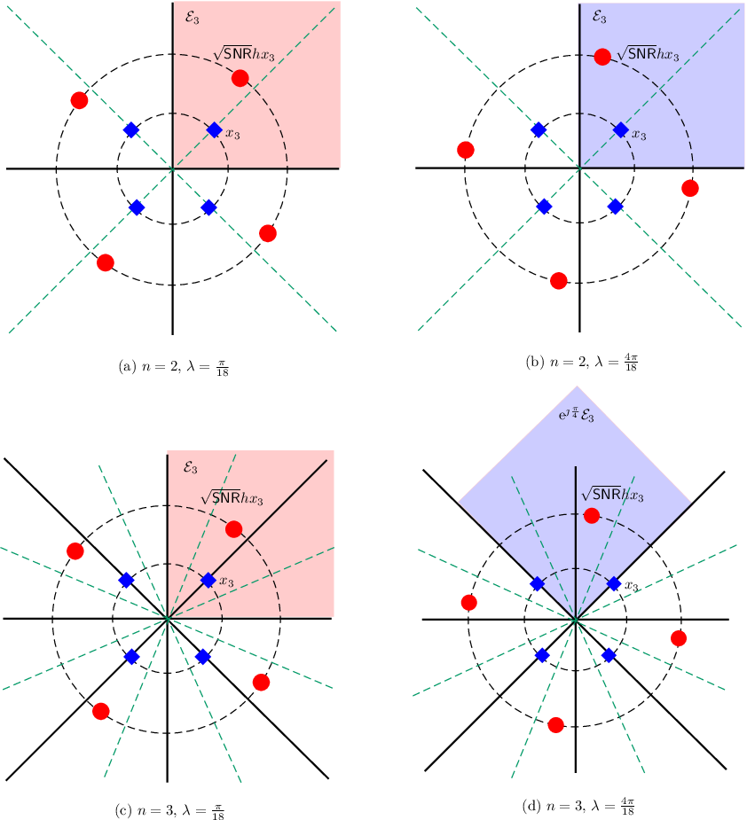
Let us consider an example for QPSK modulation with $2$-bit and $3$-bit quantization. Without loss of generality, we will assume that $x_{3}={\rm e}^{\jmath\frac{\pi}{M}}$ is the transmitted signal. Our analysis will be for two cases of $\lambda=\frac{\pi}{18}$ and $\lambda=\frac{4\pi}{18}$, where $\lambda=\mathsf{Arg}\left(h\right)$. Table I summarizes these two cases, and Fig. 3 illustrates them. In this figure, we show both the original signal points (indicated by ‘$\diamond$’) and the rotated ones (indicated by ‘$\bullet$’) after multiplying with $\sqrt{\mathsf{SNR}}$ and $h$.

For both $2$-bit and $3$-bit quantization, we observe that $h\in\mathcal{D}_{2}$ and $h\in\mathcal{D}_{4}$ for $\lambda=\frac{\pi}{18}$ and $\lambda=\frac{4\pi}{18}$, respectively. Therefore, for $2$-bit quantization, the region of attraction for $x_{3}$ will be $\mathcal{E}_{3}$ for both cases. Here, we can see that the rotated constellation point $\sqrt{\mathsf{SNR}}hx_{3}$ is very close to the decision boundary when $\lambda=\frac{4\pi}{18}$. Hence, there is a high probability that the received signal $\sqrt{\mathsf{SNR}}hx_{3}+w$ lands in the adjacent quantization region for $\lambda=\frac{4\pi}{18}$. In this instance, we will have a detection error. However, with the addition of one bit to the quantizer (i.e. with $3$-bit quantization), the region of attraction of $x_{3}$ will be ${\rm e}^{\jmath\frac{\pi}{4}}\mathcal{E}_{3}$, and hence the ML detector can correctly decode the transmitted signal even if the received one lands in the adjacent quantization region. This is illustrated in Fig. 3(d). Therefore, the addition of one extra bit to the quantizer, steers the received signal away from the error-prone decision boundaries to improve $p\left(\mathsf{SNR}\right)$. Similarly, when the number of bits in the quantizer continues to increase, the quantization regions will become thinner, and hence the regions of attraction will be better centered around the received signal points. This is the fundamental phenomenon that explains why the average $\mathsf{SEP}$ improves with a larger number of quantization bits.

Nakagami-$m$ Fading: In the special case of QPSK modulation (i.e., $M=4$), the average $\mathsf{SEP}$ expression in (3) can be further simplified to produce

because $\tan\left(\frac{2\pi}{M}\right)=\infty$ for $M=4$. By using hypergeometric function ${}_{2}F_{1}[\cdot]$ [39], we can simplify (30) for 2-bit quantization (i.e., $M=4$ and $n=2$) as

Rayleigh Fading: For special case of Rayleigh fading, which is obtained by setting $m=1$, the expression in (30) can be re-expressed as

References

• [1] Q. Bai and J. A. Nossek, “Energy efficiency maximization for 5G multi-antenna receivers,” Trans. Emerging Telecommunications Technologies, vol. 26, pp. 3–14, 2015.
• [2] S. Rangan, T. S. Rappaport, and E. Erkip, “Millimeter-wave cellular wireless networks: Potentials and challenges,” Proc. IEEE, vol. 102, no. 3, pp. 366–385, Mar. 2014.
• [3] B. Murmann, “ADC performance survey 1997-2017.” [Online]. Available: http://web.stanford.edu/ murmann/adcsurvey.htm
• [4] J. Zhang, L. Dai, X. Li, Y. Liu, and L. Hanzo, “On low-resolution ADCs in practical 5G millimeter-wave massive MIMO systems,” IEEE Commun. Mag., vol. 56, no. 7, pp. 205–211, Jul. 2018.
• [5] M. T. Ivrlac and J. A. Nossekh, “On MIMO channel estimation with single-bit signal-quantization,” in Proc. Int. ITG/IEEE Workshop on Smart Antennas (WSA), Vienna, Austria, Feb. 2007.
• [6] T. M. Lok and V. K.-W. Wei, “Channel estimation with quantized observations,” in Proc. 1998 IEEE International Symposium on Information Theory, Aug. 1998, pp. 333–333.
• [7] J. Singh, S. Ponnuru, and U. Madhow, “Multi-gigabit communication: the adc bottleneck1,” in 2009 IEEE International Conference on Ultra-Wideband, Vancouver, Canada, Sep. 2009, pp. 22–27.
• [8] O. Dabeer and U. Madhow, “Channel estimation with low-precision analog-to-digital conversion,” in 2010 IEEE International Conference on Communications, Cape Town, South Africa, May 2010, pp. 1–6.
• [9] J. Mo, P. Schniter, N. G. Prelcic, and R. W. Heath, “Channel estimation in millimeter wave MIMO systems with one-bit quantization,” in Proc. 48th Asilomar Conference on Signals, Systems and Computers, Pacific Grove, California, Nov. 2014, pp. 957–961.
• [10] “Mobile IoT in the 5G Future.” [Online]. Available: https://www.ericsson.com/assets/local/networks/documents/gsma-5g-mobile-iot.pdf
• [11] J. Choi, D. J. Love, D. R. Brown, and M. Boutin, “Quantized distributed reception for MIMO wireless systems using spatial multiplexing,” IEEE Trans. Signal Process., vol. 63, no. 13, pp. 3537–3548, Jul. 2015.
• [12] J. Choi, J. Mo, and R. W. Heath, “Near maximum-likelihood detector and channel estimator for uplink multiuser massive MIMO systems with one-bit ADCs,” IEEE Trans. Commun., vol. 64, no. 5, pp. 2005–2018, May 2016.
• [13] J. Choi, D. J. Love, and D. R. Brown, “Channel estimation techniques for quantized distributed reception in MIMO systems,” in Proc. 48th Asilomar Conference on Signals, Systems and Computers, Pacific Grove, California, Nov. 2014, pp. 1066–1070.
• [14] Y. Li, C. Tao, G. Seco-Granados, A. Mezghani, A. L. Swindlehurst, and L. Liu, “Channel estimation and performance analysis of one-bit massive MIMO systems,” IEEE Trans. Signal Process., vol. 65, no. 15, pp. 4075–4089, Aug 2017.
• [15] A. K. Saxena, I. Fijalkow, and A. L. Swindlehurst, “On one-bit quantized ZF precoding for the multiuser massive MIMO downlink,” in Proc. 2016 IEEE Sensor Array and Multichannel Signal Processing Workshop (SAM), Rio de Janeiro, Brazil, Jul. 2016, pp. 1–5.
• [16] ——, “Analysis of one-bit quantized precoding for the multiuser massive MIMO downlink,” IEEE Trans. Signal Process., vol. 65, no. 17, pp. 4624–4634, Sep. 2017.
• [17] A. Swindlehurst, A. Saxena, A. Mezghani, and I. Fijalkow, “Minimum probability-of-error perturbation precoding for the one-bit massive MIMO downlink,” in Proc. 2017 IEEE International Conference on Acoustics, Speech and Signal Processing (ICASSP), New Orleans, USA, Mar. 2017, pp. 6483–6487.
• [18] J. Mo and R. W. Heath, “High SNR capacity of millimeter wave MIMO systems with one-bit quantization,” in Proc. 2014 Information Theory and Applications Workshop (ITA), San Diego, California, USA, Feb. 2014, pp. 1–5.
• [19] ——, “Capacity analysis of one-bit quantized MIMO systems with transmitter channel state information,” IEEE Trans. Signal Process., vol. 63, no. 20, pp. 5498–5512, Oct. 2015.
• [20] A. Mezghani and J. A. Nossek, “Analysis of 1-bit output noncoherent fading channels in the low SNR regime,” in Proc. 2009 IEEE International Symposium on Information Theory, Seoul, Korea, Jun. 2009, pp. 1080–1084.
• [21] ——, “On ultra-wideband MIMO systems with 1-bit quantized outputs: Performance analysis and input optimization,” in Proc. 2007 IEEE International Symposium on Information Theory, Nice, France, Jun. 2007, pp. 1286–1289.
• [22] Y. Li, C. Tao, A. L. Swindlehurst, A. Mezghani, and L. Liu, “Downlink achievable rate analysis in massive MIMO systems with one-bit DACs,” IEEE Commun. Lett., vol. 21, no. 7, pp. 1669–1672, Jul. 2017.
• [23] J. Singh and U. Madhow, “Phase-quantized block noncoherent communication,” IEEE Trans. Commun., vol. 61, no. 7, pp. 2828–2839, Jul. 2013.
• [24] N. Liang and W. Zhang, “Mixed-ADC massive MIMO,” IEEE J. Sel. Areas Commun., vol. 34, no. 4, pp. 983–997, April 2016.
• [25] A. Mezghani, M. S. Khoufi, and J. A. Nossek, “A modified MMSE receiver for quantized MIMO systems,” in Proc. Int. ITG/IEEE Workshop on Smart Antennas (WSA), Vienna, Austria, 2007.
• [26] A. Mezghani, M. Rouatbi, and J. A. Nossek, “An iterative receiver for quantized MIMO systems,” in Proc. 2012 16th IEEE Mediterranean Electrotechnical Conference, Yasmine Hammamet, Tunisia, Mar. 2012, pp. 1049–1052.
• [27] S. Krone and G. Fettweis, “Fading channels with 1-bit output quantization: Optimal modulation, ergodic capacity and outage probability,” in 2010 IEEE Information Theory Workshop, Dublin, Ireland, Aug 2010, pp. 1–5.
• [28] R. G. Gallager, Principles of Digital Communication. New York, NY, USA: Cambridge University Press, 2008.
• [29] R. Remmert, Theory of Complex Functions. New York: Springer-Verlag, 1991.
• [30] B. Picinbono, “On circularity,” IEEE Trans. Signal Process., vol. 42, no. 12, pp. 3473–3482, Dec. 1994.
• [31] E. Ollila, D. E. Tyler, V. Koivunen, and H. V. Poor, “Complex elliptically symmetric distributions: Survey, new results and applications,” IEEE Trans. Signal Process., vol. 60, no. 11, pp. 5597–5625, Nov. 2012.
• [32] A. Mezghani, F. Antreich, and J. A. Nossek, “Multiple parameter estimation with quantized channel output,” in Proc. 2010 International ITG Workshop on Smart Antennas (WSA), Feb 2010, pp. 143–150.
• [33] J. Mo, P. Schniter, and R. W. Heath, “Channel estimation in broadband millimeter wave MIMO systems with few-bit ADCs,” IEEE Trans. Signal Process., vol. 66, no. 5, pp. 1141–1154, March 2018.
• [34] C. Wen, C. Wang, S. Jin, K. Wong, and P. Ting, “Bayes-optimal joint channel-and-data estimation for massive MIMO with low-precision ADCs,” IEEE Trans. Signal Process., vol. 64, no. 10, pp. 2541–2556, May 2016.
• [35] T. M. Cover and J. A. Thomas, Elements of Information Theory. New York, NY, USA: John Wiley & Sons, 1991.
• [36] F. D. Neeser and J. L. Massey, “Proper complex random processes with applications to information theory,” IEEE Trans. Inf. Theory, vol. 39, no. 4, pp. 1293–1302, Jul. 1993.
• [37] M. Nakagami, “The mm-distribution - A general formula of intensity distribution of rapid fading,” Statistical Methods in Radio Wave Propagation - Pergamon Press, pp. 7–36, 1960.
• [38] G. L. Stüber, Principles of Mobile Communication (2Nd Ed.), 2nd ed. Norwell, MA, USA: Kluwer Academic Publishers, 2001.
• [39] I. S. Gradshteyn and I. M. Ryzhik, Table of integrals, series, and products, 7th ed. Elsevier/Academic Press, Amsterdam, 2007.
• [40] N. C. Beaulieu and C. Cheng, “Efficient nakagami-m fading channel simulation,” IEEE Trans. Veh. Technol., vol. 54, no. 2, pp. 413–424, Mar. 2005.
• [41] W. Rudin, Real and Complex Analysis, 3rd ed. New York: McGraw-Hill, 1987.
• [42] R. H. Walden, “Analog-to-digital converter survey and analysis,” IEEE J. Sel. Areas Commun., vol. 17, no. 4, pp. 539–550, Apr. 1999.
• [43] R. W. Lucky and J. C. Hancock, “On the optimum performance of nn-ary systems having two-degrees of freedom,” IRE Trans. Commun. Syst., vol. 10, no. 2, pp. 185–192, Jun. 1962.
• [44] D. P. Bertsekas and J. N. Tsitsiklis, Introduction to Probability, 2nd ed. Nashua: Athena Scientific, 2008.
• [45] K. T. Fang, S. Kotz, and K. W. Ng, Symmetric Multivariate and Related Distributions, 1st ed. New York: CRC Press, 1990.