Convergence and Applications of ADMM on the Multi-convex Problems
Abstract
In recent years, although the Alternating Direction Method of Multipliers (ADMM) has been empirically applied widely to many multi-convex applications, delivering an impressive performance in areas such as nonnegative matrix factorization and sparse dictionary learning, there remains a dearth of generic work on proposed ADMM with a convergence guarantee under mild conditions. In this paper, we propose a generic ADMM framework with multiple coupled variables in both objective and constraints. Convergence to a Nash point is proven with a sublinear convergence rate . Two important applications are discussed as special cases under our proposed ADMM framework. Extensive experiments on ten real-world datasets demonstrate the proposed framework’s effectiveness, scalability, and convergence properties. We have released our code at https://github.com/xianggebenben/miADMM.
1 Introduction
Due to the advantages and popularity of non-differentiable regularized and distributive computing for complex optimization problems, the Alternating Direction Method of Multipliers (ADMM) has received a great deal of attention in recent years [6]. The standard ADMM was originally proposed to solve the following separable convex optimization problem:
where and are closed convex functions, and are matrices and is a vector. There are extensive reports in the literature exploring the theoretical properties for convex optimization problems related to ADMM and its variants, including multi-block ADMM [12], Bregman ADMM [30], fast ADMM [14, 18], and stochastic ADMM [24]. ADMM has now been extended to cover a wide range of nonconvex problems, and it has achieved outstanding performance in many practical applications [40].
Unlike convex problems, the convergence theory on the nonconvex ADMM is much more difficult, and considerable progress has been made on this problem, please refer to Section 2 for a detailed summary.
Recently, however, there has been an increasing number of real-world applications where the objective functions are multi-convex (i.e. nonconvex for all the variables but convex for each when all the others are fixed). For example, nonnegative matrix factorization, which aims to decompose a matrix into a product of two matrices, has been applied widely in computer vision, machine learning, and various other fields [19]; A bilinear matrix inequality problem has been designed for the analysis of linear and nonlinear uncertain systems [16].
All of the above applications can be considered as special cases of multi-convex optimization problems. However, such problems have not yet been rigorously and systematically investigated by ADMM. Moreover, the convergence properties of the ADMM required to solve such problems remain unknown. In this work, we propose mild conditions to ensure the convergence of ADMM to a Nash point on the multi-convex problems with a sublinear convergence rate . We also discuss how our ADMM is applied to two important applications. Extensive experiments show the effectiveness of our proposed ADMM. Our contributions in this paper include:
- •
We propose an ADMM framework to solve the multi-convex problem, and we investigate the convergence properties of the proposed ADMM. Specifically, we prove that the objective value and the residual are convergent. Moreover, any limit point generated by the proposed ADMM is a Nash point of the original problem. The convergence rate of the proposed ADMM is .
- •
We demonstrate two important and promising applications that are special cases of our proposed ADMM framework and benefit from its theoretical properties. Specifically, we show how these applications can be transformed equivalently to fit into the proposed ADMM framework.
- •
We conduct extensive experiments to validate our proposed ADMM. Experiments on ten real-world datasets demonstrate its effectiveness, scalability, and convergence properties.
The rest of this paper is summarized as follows: Section 2 summarizes previous work related to this paper. Section 3 introduces the ADMM algorithm and its convergence properties. In Section 4, the proposed ADMM algorithm is applied to several important applications. Extensive experiments are described in Section 5. The paper concludes with a summary of the work in Section 6.
2 Related Work
Multi-convex optimization problems: Some works studied multi-convex problems. The earliest work required that the objective function was differentiable continuous and strictly convex [38]. Various conditions on separability and regularity on the objective functions have been discussed in [28, 29]. In the most recent work, Xu and Yin presented three types of multi-convex algorithms and analyzed convergence based on either Lipschitz differentiability or strong convexity assumption [39]. For a comprehensive survey, please refer to [26].
Convergence analysis of
ADMM: Existing literature on the convergence analysis of ADMM can be categorized into two classes: the convex ADMM and the nonconvex ADMM. The convex ADMM is investigated relatively well compared with the nonconvex ADMM. Existing works either study suitable stepsizes of the convex ADMM or extend ADMM to the stochastic version. For example, Bai et al. proposed a generalized symmetric ADMM to solve the multi-block separable objective by updating the Lagrange multiplier twice with suitable stepsizes [3]; Gu et al. extended contractive Peaceman-Rachford splitting method to ADMM with larger stepsizes [15]; Ouyang et al. proposed a stochastic ADMM with a convergence rate . Despite the outstanding performance of the nonconvex ADMM, its convergence theory is not well established due to the complexity of both coupled objectives and various (inequality and equality) constraints. Most existing works discussed the convergence of the nonconvex ADMM on separable objectives: they provided convergence guarantee to the stationary solutions with different assumptions [5, 9, 10, 20]. Some works explored more difficult cases where the objectives are coupled: for example, Wang et al. presented mild convergence conditions of the nonconvex ADMM where the objective can be nonsmooth [37]; Gao et al. explored the convergence condition of ADMM on multi-affine constraints [13]; Wang et al. gave the convergence proofs of ADMM in the nonconvex deep learning problems [31, 33, 34]; while experiments by Wang and Zhao showed that the ADMM was not necessarily convergent in the nonlinear-constrained problems [35].
3 ADMM on the Multi-convex Problems
In this section, we present an ADMM framework to solve Problem 1.
3.1 Preliminaries
First, the definition of Lipschitz differentiability is shown as follows [8]:
Definition 1 (Lipschitz Differentiability)
Any arbitrary differentiable function is Lipschitz differentiable if for any ,
where is constant and denotes the gradient of .
The following defines strong convexity, which is indispensable for the proof of convergence to a Nash point.
Definition 2 (Strong Convexity)
A convex function is strongly convex if there exists such that for , the following holds
where is a subdifferential of at .
Finally, the Nash point is defined as follows [39]:
Definition 3 (Nash Point)
Given , a Nash point satisfies the following property:
Naturally, when we optimize one variable while fixing others, the Nash point ensures the optimality of this variable [39]. Without loss of generality, we assume that Problem 1 has at least a Nash point, and in the next section, we will prove that any limit point generated by ADMM converges to a Nash point.
3.2 The ADMM algorithm
The following problem is our focus in this paper:
Problem 1
where , , are proper, continuous, multi-convex and possibly nonsmooth functions, is a proper, differentiable and convex function. are matrices. Obviously, the domain of is . Without the loss of generality, the objective of Problem 1 is assumed to be bounded from below.
To ensure the convergence of the proposed ADMM, some mild assumptions are imposed, which are shown as follows:
Assumption 1 (Lipschitz Differentiability)
is Lipschitz differentiable with constant .
Most loss functions such as the cross-entropy loss and the square loss are Lipschitz differentiable [34]. In order to propose the ADMM algorithm, the augmented Lagrangian function can be formulated mathematically as follows:
| (1) |
where is a dual variable and is a penalty parameter. The proposed ADMM aims to optimize the following subproblems alternately.
| (2) | ||||
| (3) | ||||
Algorithm 1 is presented for Problem 1. Concretely, Lines 3-5 and 6 update and , respectively. Line 7 updates the primal residual , which is defined in accordance with the standard ADMM [6]: it measures how the linear constraint is violated. Line 8 updates the dual variable , which follows the routine of the standard ADMM. Line 10 uses the norm of the primal residual as a condition to terminate the algorithm, where is a threshold. Each subproblem is convex and implicitly assumed to be solvable.
3.3 Convergence Analysis
This section focuses on the convergence of the proposed ADMM algorithm. Specifically, the first lemma states that the augmented Lagrangian keeps decreasing, which is stated as follows.
Lemma 1 (Objective Descent)
If so that , then there exists such that
| (4) |
Lemma 1 holds under Assumption 1, and its proof can be found in Section 0.B in the supplementary materials11 1 The supplementary materials are available at https://github.com/xianggebenben/miADMM/blob/main/multi_convex_ADMM-13-18.pdf. The next lemma states that the augmented Lagrangian is bounded from below, as shown below:
Lemma 2 (Objective Bound)
If , then is lower bounded.
The proof of Lemma 2 can be found in Section 0.B in the supplementary materials 1. Now we can prove that the proposed ADMM converges globally in the following theorem.
Theorem 3.1 (Residual and Objective Convergence)
If , then for the bounded sequence , then it has the following properties:
a). Residual convergence. This means that as , , where is defined in Algorithm 1.
b). Objective convergence. This means that as , converges.
Theorem 3.1 guarantees the convergence of the proposed ADMM, whose proof is in Section 0.C in the supplementary materials 1. However, and are not necessarily shown to be convergent. The next theorem states that any limit point is a feasible Nash Point of Problem 1.
Theorem 3.2 (Convergence to a Nash Point)
Let , if either of two assumptions hold: (a). have full rank. (b). is strongly convex with regard to . Then for bounded variables , it has at least a limit point , and any limit point is a feasible Nash point of defined in Problem 1. That is
The proof of Theorem 3.2 is detailed in Section 0.C in the supplementary materials 1. The third theorem states that our proposed ADMM can achieve a sublinear convergence rate of under Assumption 1, despite the nonconvex and complex nature of Problem 1. Such a rate is state-of-the-art even compared to those methods for simpler convex problems. The theorem is shown as follows:
Theorem 3.3 (Convergence Rate)
If , for a bounded sequence , define , then the convergence rate of is .
The proof of this theorem is in Section 0.C in the supplementary materials 1. The convergence rate of the proposed ADMM is consistent with much existing work analyzing the convex ADMM, including [12, 17, 22]. Our contribution in term of convergence rate is that we extend the guarantee of into the multi-convex Problem 1.
Our proposed ADMM is more general than some influential works in terms of formulation. The relations between our proposed ADMM and previous works are summarized as follows:
1. Generalization of Block Coordinate Descent (BCD) for multi-convex problems. When the linear constraint is removed in Problem 1, then the proposed ADMM is reduced to the Block Coordinate Descent [39].
2. Generalization of multi-block ADMM.
When , the proposed ADMM is reduced to the convex multi-block ADMM [27], i.e. the ADMM with no less than three variables.
Apart from general formulations, the convergence guarantees of our proposed ADMM cover more applications than previous literature. For example, [37] requires the coupled objective to be Lipschitz differentiable. However, some important applications such as weakly-constrained multi-task learning (Section 4.1) and learning with signed-network constraints (Section 4.2) do not satisfy this condition. But they are covered by our convergence guarantees of the multi-convex ADMM to a Nash point.
4 Applications
In this section, we apply our proposed ADMM to two real-world applications, both of which conform to Problem 1 and benefit from the convergence properties of the proposed ADMM.
4.1 Weakly-constrained Multi-task Learning
In multi-task learning problems, multiple tasks are learned jointly to achieve a better performance compared with learning tasks independently [32]. Most work on multi-task learning has tended to enforce the assumption of similarity among the feature weight values across tasks [2, 11, 36, 32, 43] because this makes it possible to use convex regularization terms like norms [36] and Graph Laplacians [43]. However, this assumption is usually too strong and is seldom satisfied by the real-world data. Instead of requiring feature weights to be similar in magnitude, a more conservative but probably more reasonable assumption is that multiple tasks share similar polarities for the same feature, which means that if a feature is positively relevant to the output of a task, then its weight will also be positive for other related tasks. This assumption is appropriate for many applications. For example, the feature ‘number of clinic visits’ will be positively related to flu outbreaks, while the feature ‘popularity of vaccination’ will be negatively related to them, even though their feature weights can vary dramatically for different countries (namely tasks here). This is achieved by enforcing the requirement for every pair of tasks with neighboring indices to have the same weight sign. This optimization objective is shown as follows:
| (5) | ||||
where and denote the number of tasks and features, respectively, is the weight of the -th feature in the -th task, is the weight of the -th task, and and are the loss function and the regularization term of the -th task, respectively. The inequality constraint implies that the -th and the -th tasks share the same sign for their weights. Equation (5) is rewritten in the following form to fit in our proposed ADMM framework:
| (6) | ||||
where is an auxiliary variable, and is a tuning parameter. Notice that the inequality constraint is transformed to a quadratic penalty such that which makes the formulation consistent with Problem 1. The proposed ADMM algorithm for this case is shown in Appendix 0.D.1 in the supplementary materials 1.
4.2 Learning with Signed-Network Constraints
The application of network models for social network analysis has attracted the attention of a large number of researchers [7]. For example, influential societal events often spread across many social networking sites and are expressed in different languages. Such multi-lingual indicators usually transmit similar semantic information through networks and have thus been utilized to facilitate social event forecasting [41]. The problem with network constraints is formulated as follows:
where is the weight of the -th node. is a loss function and is a regularization term for the -th node. and are two edge sets to represent two opposite relationships: means that , while means that . The constraint means that some pair satisfies the edge set , and that some pair satisfies the edge set . For example, in the problem of social event forecasting with French and English, and are edge sets of synonyms and antonyms between French and English, and the weight pair of the French word ”bien” and the English word ”good” belongs to . The problem with network constraints can be reformulated approximately to the following:
| (7) |
where is an auxiliary variable, and is a tuning parameter. The constraint and are transformed to two quadratic penalties and as follows:
.
The proposed ADMM for this case is also shown in Appendix 0.D.2 in the supplementary materials 1.
5 Experiments
In this section, we test our proposed ADMM using ten real-world datasets on two applications detailed in Section 4. Scalability, effectiveness, and convergence properties are compared with several existing state-of-the-art methods on ten real datasets. All experiments were conducted on a 64-bit machine with Intel(R) Core(TM) processor (i7-6820HQ CPU@ 2.70GHZ) and 16.0GB memory.

(a). Residual on
Experiment I.
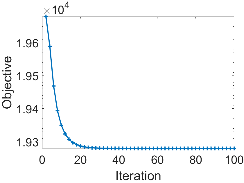
(b). Objective on
Experiment I.

(c). Residual on the VE
dataset of
Experiment II.

(d). Objective on the VE
dataset of
Experiment II.
5.1 Experiment I: Weak-constrained Multi-task Learning
To evaluate the effectiveness of our method on the application of weak-constrained multi-task learning described in Equation (6), a real-world school dataset is used to evaluate the effectiveness of our proposed ADMM. It consists of the examination scores in three years of 15,362 students
from 139 secondary schools, which are treated as tasks for examination
scores prediction based on 27 input features such as year of the examination, school-specific features, and student-specific features. The dataset is publicly available and the detailed description can be found in the original paper [21]. was set to . Here we chose two kinds of : (1) ; (2) with . and are the first and the second choice of , respectively.
Metrics. In this experiment, five metrics were utilized to evaluate model performance. Mean Squared Error (MSE) measures the average of the squares of the difference between observation and estimation. Different from MSE, Mean Squared Logarithmic Error (MSLE) measures the ratio of observation to estimation. Mean Absolute Error (MAE) is also an error measurement but computed in the absolute value. The less the above three metrics are, the better a regression model is. Explained Variance (EV) computes the ratio of the variance of the error to that of observation. The coefficient of determination or R2 score is the proportion of the variance in the dependent variable that is predictable from the independent variable. The higher score of EV and R2 are, the better a regression model is.
Baselines. To validate the effectiveness of the proposed ADMM, five benchmark multi-task learning models served as comparison methods. Loss functions were set to least square errors. The number of iterations was set to . The regularization parameter was set based on 5-fold cross-validation on the training set.
1. multi-task learning with Joint Feature Selection (JFS) [2, 43] . JFS is one of the most commonly used strategies in multi-task learning. It captures the relatedness of multiple tasks by a constraint of a weight matrix to share a common set of features. was set to 100.
2. Clustered Multi-Task Learning (CMTL) [42, 43]. CMTL assumes that multiple tasks are clustered into several groups. Tasks in the same group are similar to each other. was set to 1.
3. multi-task Lasso (mtLasso) [43]. mtLasso extends the classic Lasso model to the multi-task learning setting. was set to 10.
4. a convex relaxation of Alternating Structure Optimization (cASO) [43, 1]. cASO decomposes each task into two components: task-specific feature mapping and task-shared feature mapping. was set to 0.01.
5. Block Coordinate Descent (BCD) [39]. BCD is an intuitive method to solve multi-convex problems, which optimizes each variable alternately. was set to 10.
| Mean | |||||
| Method | MSE | MSLE | MAE | EV | R2 |
| JFS | 114.1052 | 0.4531 | 8.4349 | 0.2948 | 0.2948 |
| CMTL | 114.9892 | 0.4647 | 8.4756 | 0.2876 | 0.2875 |
| mtLasso | 115.3143 | 0.4625 | 8.4725 | 0.2873 | 0.2873 |
| cASO | 137.8336 | 0.5204 | 9.3450 | 0.1606 | 0.1605 |
| BCD | 149.2313 | 0.5577 | 9.8057 | 0.1299 | 0.0777 |
| ADMM() | 113.6975 | 0.4423 | 8.4024 | 0.2950 | 0.2960 |
| ADMM() | 113.2400 | 0.4428 | 8.3943 | 0.3002 | 0.3002 |
| Standard Deviation | |||||
| Method | MSE | MSLE | MAE | EV | R2 |
| JFS | 2.02 | 0.02 | 0.06 | 0.02 | 0.02 |
| CMTL | 1.85 | 0.02 | 0.05 | 0.01 | 0.01 |
| mtLasso | 1.77 | 0.02 | 0.05 | 0.01 | 0.01 |
| cASO | 7.26 | 0.01 | 0.06 | 0.01 | 0.01 |
| BCD | 1.41 | 0.01 | 0.06 | 0.15 | 0.01 |
| ADMM() | 0.83 | 0.005 | 0.03 | 0.01 | 0.01 |
| ADMM() | 0.95 | 0.01 | 0.04 | 0.02 | 0.02 |
Performance.
As discussed in Section 4.1, the convergence of our proposed ADMM is guaranteed based on our theoretical framework. To verify this, Figures 1(a) and 1(b) illustrate the residual and objective values in different iterations, which demonstrates the convergence of the proposed ADMM on this nonconvex problem. Then the performance of examination score prediction on this dataset is illustrated in Table 1. Table 1 shows the mean and the standard deviation of all methods, which were repeated 10 times by initializing parameters randomly, to make experimental evaluation robust. It shows that outperforms in four out of five metrics for the proposed ADMM. In addition, the proposed ADMM achieves the best performance in all the metrics, compared to all comparison methods. Moreover, the standard deviation of the proposed ADMM is about smaller than any other comparison method. This is because our method only enforces that the sign of the feature weight across different tasks is the same, while comparison methods typically perform too aggressive assumptions on the similarity among tasks. For example, CMTL enforces that the correlated tasks need to have similar feature weights using squared regularization on the difference between feature weights. JFS and mtLasso still tend to enforce similar weights on features in different tasks by norm. Because their enforcement is weaker than CMTL, their performance is better. cASO gets relatively weak performance because it optimizes an approximation of a nonconvex problem, and thus the approximate solution may be distant from the true solution to the original problem. Finally, the BCD performs the worst among all methods, even though it shares the same formulation with our proposed ADMM. This reflects the advantage of our proposed ADMM algorithm: dual information in one iteration can be passed to its following iteration by dual variables, which yields better performance.

Scalability. To investigate the scalability of the proposed ADMM compared with all baselines in Experiment I, we measured the training time of them in the school dataset when the number of features varies. The training time was averaged by running 20 times. Figure 2 shows the training time of all methods when the number of features ranges from 10 to 28. The training time of all methods increased linearly concerning the number of features. cASO was the most efficient of all methods, while the proposed ADMM was ranked second. mtLasso and JFS also trained a model within 5 seconds on average. CMTL was time-consuming for training, which spent more than 10 seconds.
5.2 Experiment II: Event Forecasting with Multi-lingual Indicators
Datasets.
To evaluate the performance of our proposed ADMM on the application in Section 4.2, extensive experiments on nine real-world datasets have been performed. The dataset is obtained by randomly
sampling 10% (by volume) of the Twitter data from Jan 2013 to Dec 2014. The data in the first and second years are used and training and test set, respectively. For the topic (i.e., social unrest) of interest, 1,806 keywords in the three major languages in Latin America, namely English, Spanish, and Portuguese, were provided by the paper [41]. Their translation relationships have also been labeled as semantic links among them, such as “protest” in English, “protesta” in Spanish, and “protesto” in Portuguese. The event forecasting results were validated against a labeled event set, known as the Gold Standard Report (GSR), which is publicly available [25].
Metric and Baselines.
The metric used to evaluate the performance is Area Under the receiver operating characteristic Curve (AUC). Five comparison methods including the state-of-the-art Multi-Task learning (MTL), Multi-Resolution Event Forecasting (MREF), and Distant-supervision of Heterogeneous Multitask Learning (DHML) as well as classic methods Logistic Regression (LogReg) and Lasso. was set to . Here we chose two kinds of : (1) ; (2) with . and are the first and the second choice of , respectively. All the hyper-parameters were tuned by 5-fold cross-validation.
| BR | CL | CO | EC | EL | MX | PY | UY | VE | |
|---|---|---|---|---|---|---|---|---|---|
| LogReg | 0.686 | 0.677 | 0.644 | 0.599 | 0.618 | 0.661 | 0.616 | 0.628 | 0.667 |
| LASSO | 0.685 | 0.677 | 0.648 | 0.603 | 0.636 | 0.665 | 0.615 | 0.666 | 0.669 |
| MTL | 0.722 | 0.669 | 0.810 | 0.617 | 0.772 | 0.795 | 0.600 | 0.811 | 0.771 |
| MREF | 0.714 | 0.563 | 0.515 | 0.784 | 0.612 | 0.693 | 0.658 | 0.681 | 0.588 |
| DHML | 0.845 | 0.683 | 0.846 | 0.839 | 0.780 | 0.793 | 0.737 | 0.835 | 0.835 |
| BCD | 0.847 | 0.668 | 0.850 | 0.830 | 0.773 | 0.800 | 0.736 | 0.835 | 0.856 |
| ADMM | 0.864 | 0.699 | 0.870 | 0.848 | 0.794 | 0.820 | 0.746 | 0.850 | 0.867 |
| ADMM | 0.867 | 0.701 | 0.872 | 0.851 | 0.798 | 0.823 | 0.747 | 0.847 | 0.865 |
Performance. As shown in Table 2, outperforms marginally in seven out of nine datasets for the proposed ADMM, and they generally perform the best among all the methods, with DHML and BCD the second-best performer. They all outperform the others typically by at least 5%-10%. This is because they leverage the multilingual correlation among the features to boost up the model’s generalizability. Thanks to the framework of multi-task learning, MTL and MREF obtained a competitive performance with AUC typically over 0.7, which outperforms simple methods like LogReg and LASSO by 5% on average.
| LogReg | LASSO | MTL | MREF | DHML | ADMM | |
|---|---|---|---|---|---|---|
| BR | 30193 | 1535 | 233 | 25889 | 332 | 14 |
| CL | 2981 | 242 | 35 | 6521 | 852 | 11 |
| CO | 8060 | 780 | 108 | 14714 | 87 | 31 |
| EC | 312 | 295 | 17 | 4332 | 46 | 25 |
| EL | 551 | 261 | 17 | 4669 | 33 | 3 |
| MX | 17712 | 2043 | 853 | 31349 | 175 | 29 |
| PY | 7297 | 527 | 40 | 9495 | 242 | 5 |
| UY | 748 | 336 | 20 | 5305 | 82 | 3 |
| VE | 5563 | 1008 | 49 | 5769 | 179 | 28 |
Efficiency. In Experiment II, we also compared the training time of the proposed ADMM in comparison with all baselines on 9 datasets. The training time was averaged by running 5 times. The training time was shown in Table 3. We do not show BCD because its training time is similar to the proposed ADMM. Overall, the proposed ADMM was the most efficient of all methods for all datasets. It consumed no more than 30 seconds on all datasets. MTL ranked second, but it spent hundreds of seconds on some datasets, like BR and MX. As the most time-consuming baselines, LogReg and MREF trained a model in thousands of seconds or more.
6 Conclusions
We propose an ADMM framework for multi-convex problems with multiple coupled variables. It not only inherits the merits of general ADMMs but also provides advantageous theoretical properties on convergence conditions and properties under mild conditions. Besides, several machine learning applications of recent interest are discussed as special cases of our proposed ADMM. Extensive experiments have been conducted on ten real-world datasets, and demonstrate the effectiveness, scalability, and convergence properties of our proposed ADMM.
Acknowledgement
This work was supported by the National Science Foundation (NSF) Grant No. 1755850, No. 1841520, No. 2007716, No. 2007976, No. 1942594, No. 1907805, a Jeffress Memorial Trust Award, Amazon Research Award, NVIDIA GPU Grant, and Design Knowledge Company (subcontract No: 10827.002.120.04).
References
- [1] Rie Kubota Ando and Tong Zhang. A framework for learning predictive structures from multiple tasks and unlabeled data. Journal of Machine Learning Research, 6(Nov):1817–1853, 2005.
- [2] Andreas Argyriou, Theodoros Evgeniou, and Massimiliano Pontil. Multi-task feature learning. Advances in neural information processing systems, pages 41–48, 2007.
- [3] Jianchao Bai, Jicheng Li, Fengmin Xu, and Hongchao Zhang. Generalized symmetric ADMM for separable convex optimization. Computational optimization and applications, 70(1):129–170, 2018.
- [4] Amir Beck and Marc Teboulle. A fast iterative shrinkage-thresholding algorithm for linear inverse problems. SIAM journal on imaging sciences, 2(1):183–202, 2009.
- [5] Radu Ioan Boţ and Dang-Khoa Nguyen. The proximal alternating direction method of multipliers in the nonconvex setting: convergence analysis and rates. Mathematics of Operations Research, 45(2):682–712, 2020.
- [6] Stephen Boyd, Neal Parikh, Eric Chu, Borja Peleato, and Jonathan Eckstein. Distributed optimization and statistical learning via the alternating direction method of multipliers. Foundations and Trends® in Machine Learning, 3(1):1–122, 2011.
- [7] Peter J Carrington, John Scott, and Stanley Wasserman. Models and methods in social network analysis, volume 28. Cambridge university press, 2005.
- [8] Fabio Cavalletti and Tapio Rajala. Tangent lines and lipschitz differentiability spaces. Analysis and Geometry in Metric Spaces, 4(1):85–103, 2016.
- [9] MT Chao, Y Zhang, and JB Jian. An inertial proximal alternating direction method of multipliers for nonconvex optimization. International Journal of Computer Mathematics, 98(6):1199–1217, 2021.
- [10] Rick Chartrand and Brendt Wohlberg. A nonconvex ADMM algorithm for group sparsity with sparse groups. Acoustics, Speech and Signal Processing (ICASSP), 2013 IEEE International Conference on, pages 6009–6013, 2013.
- [11] Jianhui Chen, Jiayu Zhou, and Jieping Ye. Integrating low-rank and group-sparse structures for robust multi-task learning. Proceedings of the 17th ACM SIGKDD international conference on Knowledge discovery and data mining, pages 42–50, 2011.
- [12] Wei Deng, Ming-Jun Lai, Zhimin Peng, and Wotao Yin. Parallel multi-block ADMM with o (1/k) convergence. Journal of Scientific Computing, 71(2):712–736, 2017.
- [13] Wenbo Gao, Donald Goldfarb, and Frank E Curtis. ADMM for multiaffine constrained optimization. Optimization Methods and Software, 35(2):257–303, 2020.
- [14] Tom Goldstein, Brendan O’Donoghue, Simon Setzer, and Richard Baraniuk. Fast alternating direction optimization methods. SIAM Journal on Imaging Sciences, 7(3):1588–1623, 2014.
- [15] Yan Gu, Bo Jiang, and Deren Han. A semi-proximal-based strictly contractive peaceman-rachford splitting method. arXiv preprint arXiv:1506.02221, pages 1–20, 2015.
- [16] Arash Hassibi, Jonathan How, and Stephen Boyd. A path-following method for solving bmi problems in control. American Control Conference, 1999. Proceedings of the 1999, 2:1385–1389, 1999.
- [17] Bingsheng He and Xiaoming Yuan. On the o(1/n) convergence rate of the douglas–rachford alternating direction method. SIAM Journal on Numerical Analysis, 50(2):700–709, 2012.
- [18] Mojtaba Kadkhodaie, Konstantina Christakopoulou, Maziar Sanjabi, and Arindam Banerjee. Accelerated alternating direction method of multipliers. Proceedings of the 21th ACM SIGKDD international conference on knowledge discovery and data mining, pages 497–506, 2015.
- [19] Daniel D Lee and H Sebastian Seung. Algorithms for non-negative matrix factorization. Advances in neural information processing systems, pages 556–562, 2001.
- [20] Guoyin Li and Ting Kei Pong. Global convergence of splitting methods for nonconvex composite optimization. SIAM Journal on Optimization, 25(4):2434–2460, 2015.
- [21] Ya Li, Xinmei Tian, Tongliang Liu, and Dacheng Tao. Multi-task model and feature joint learning. International Joint Conference on Artificial Intelligence, pages 3643–3649, 2015.
- [22] Tian-Yi Lin, Shi-Qian Ma, and Shu-Zhong Zhang. On the sublinear convergence rate of multi-block ADMM. Journal of the Operations Research Society of China, 3(3):251–274, 2015.
- [23] Nelson Merentes and Kazimierz Nikodem. Remarks on strongly convex functions. Aequationes mathematicae, 80(1-2):193–199, 2010.
- [24] Hua Ouyang, Niao He, Long Tran, and Alexander Gray. Stochastic alternating direction method of multipliers. International Conference on Machine Learning, pages 80–88, 2013.
- [25] Terry Reed. Open source indicators project: https://doi.org/10.7910/DVN/EN8FUW, 2017.
- [26] Xinyue Shen, Steven Diamond, Madeleine Udell, Yuantao Gu, and Stephen Boyd. Disciplined multi-convex programming. Control And Decision Conference (CCDC), 2017 29th Chinese, pages 895–900, 2017.
- [27] Min Tao and Xiaoming Yuan. Convergence analysis of the direct extension of ADMM for multiple-block separable convex minimization. Advances in Computational Mathematics, 44(3):773–813, 2018.
- [28] Paul Tseng. Dual coordinate ascent methods for non-strictly convex minimization. Mathematical programming, 59(1-3):231–247, 1993.
- [29] Paul Tseng. Convergence of a block coordinate descent method for nondifferentiable minimization. Journal of optimization theory and applications, 109(3):475–494, 2001.
- [30] Huahua Wang and Arindam Banerjee. Bregman alternating direction method of multipliers. Advances in Neural Information Processing Systems, pages 2816–2824, 2014.
- [31] Junxiang Wang, Zheng Chai, Yue Cheng, and Liang Zhao. Toward model parallelism for deep neural network based on gradient-free ADMM framework. 2020 IEEE International Conference on Data Mining (ICDM), pages 591–600, 2020.
- [32] Junxiang Wang, Yuyang Gao, Andreas Züfle, Jingyuan Yang, and Liang Zhao. Incomplete label uncertainty estimation for petition victory prediction with dynamic features. 2018 IEEE International Conference on Data Mining (ICDM), pages 537–546, 2018.
- [33] Junxiang Wang, Hongyi Li, Zheng Chai, Yongchao Wang, Yue Cheng, and Liang Zhao. Towards quantized model parallelism for graph-augmented mlps based on gradient-free admm framework. arXiv preprint arXiv:2105.09837, 2021.
- [34] Junxiang Wang, Fuxun Yu, Xiang Chen, and Liang Zhao. ADMM for efficient deep learning with global convergence. Proceedings of the 25th ACM SIGKDD International Conference on Knowledge Discovery & Data Mining, pages 111–119, 2019.
- [35] Junxiang Wang and Liang Zhao. Nonconvex generalization of alternating direction method of multipliers for nonlinear equality constrained problems. Results in Control and Optimization, page 100009, 2021.
- [36] Lu Wang, Yan Li, Jiayu Zhou, Dongxiao Zhu, and Jieping Ye. Multi-task survival analysis. 2017 IEEE International Conference on Data Mining (ICDM), pages 485–494, 2017.
- [37] Yu Wang, Wotao Yin, and Jinshan Zeng. Global convergence of ADMM in nonconvex nonsmooth optimization. Journal of Scientific Computing, 78(1):29–63, 2019.
- [38] Jack Warga. Minimizing certain convex functions. Journal of the Society for Industrial and Applied Mathematics, 11(3):588–593, 1963.
- [39] Yangyang Xu and Wotao Yin. A block coordinate descent method for regularized multiconvex optimization with applications to nonnegative tensor factorization and completion. SIAM Journal on imaging sciences, 6(3):1758–1789, 2013.
- [40] Zheng Xu, Soham De, Mario Figueiredo, Christoph Studer, and Tom Goldstein. An empirical study of ADMM for nonconvex problems. NIPS 2016 Workshop on Nonconvex Optimization for Machine Learning: Theory and Practice, 2016.
- [41] Liang Zhao, Junxiang Wang, and Xiaojie Guo. Distant-supervision of heterogeneous multitask learning for social event forecasting with multilingual indicators. Proceedings of the AAAI Conference on Artificial Intelligence, 32(1), Apr. 2018.
- [42] Jiayu Zhou, Jianhui Chen, and Jieping Ye. Clustered multi-task learning via alternating structure optimization. Advances in neural information processing systems, pages 702–710, 2011.
- [43] Jiayu Zhou, Jianhui Chen, and Jieping Ye. Malsar: Multi-task learning via structural regularization. Arizona State University, 21, 2011.
Appendix
Appendix 0.A Preliminary Lemmas
In this section, we give preliminary lemmas which are also used in the proof the proofs of Lemmas 1 and 2. While Lemmas 4 and 5 depend on the optimality conditions of subproblems, Lemmas 3, 6 and 7 require Assumption 1.
Lemma 3
It holds that ,
Proof
Lemma 4
It holds that for all .
Proof
The optimality condition for the problem with regard to gives rise to
Because , we have .
Lemma 5
It holds that for ,
| (8) |
Proof
where the second equality follows from the cosine rule: with , and .
The optimality condition of leads to
We have the following result according to the definition of subgradient
Therefore, the lemma is proved.
Lemma 6
If so that , then it holds that
| (9) |
Proof
Lemma 7
, we have .
Proof
Appendix 0.B Proofs of Lemmas 1- 2
Appendix 0.C Proofs of Theorems 3.1-3.3
Proof (Proof of Theorem 3.1)
We show residual convergence and objective convergence based on Lemmas 1 and 2.
From Lemma 1, decreases monotonically, and is lower bounded by Lemma 2. Therefore, is convergent because a monotone bounded sequence converges (Monotone Convergence Theorem). According to the continuity of , we take on the both sides of Inequality (4) to obtain
On one hand, is convergent, so we have
On the other hand, is nonnegative, so we get
This suggests that and . Moreover, by Lemma 7, . So we have .
a). For residual convergence, by the Line 8 of Algorithm 1, we have
b). For objective convergence, since
and is convergent, converges to 0 and is bounded, then is also convergent.
Proof (Proof of Theorem 3.2)
Obviously and from the proof of Theorem 3.1. In order to prove this theorem, we firstly prove that if either of two assumptions holds, then prove that any limit point is a feasible Nash point of Problem 1.
(a). Suppose have full rank. Because from the proof of Theorem 3.1, then obviously [22].
(b). Suppose is strongly convex with regard to . Because , , and are strongly convex, is also strongly convex regard to [23] with the assumed constant . We have
where . The optimality condition of leads to
. Therefore, we have
| (10) |
We sum up Inequality (10) from and Inequality (9) to obtain
| (11) |
where by Lemma 6 if . According to the continuity of , we take on the both sides of Inequality (11) to obtain
On one hand, is convergent, so we have
On the other hand, is nonnegative, so we get
This suggests that and .
Therefore, if either of two assumptions holds.
Because is bounded, there exists a subsequence such that where is a limit point. Because , and , we have . Now we prove that the limit point is a feasible Nash point of Problem 1.
For feasibility, since , so for the subsequence , we have then .
For the Nash point, we obtain the following according to the optimality conditions of and in Equations (2) and (3), respectively.
According to the continuity of , we take on the both sides of two inequalities. Because and , we have
Here and mean and , respectively. Using the fact that is feasible in Problem 1, we obtain , and . Therefore, we prove that is a feasible Nash point of defined in Problem 1.
Proof (Proof of Theorem 3.3)
To prove this theorem, we will first show that satisfies two conditions: (1). . (2). is bounded. We then conclude the convergence rate of based on these two conditions. Specifically, first, we have
Therefore satisfies the first condition. Second,
where . So is bounded and satisfies the second condition. Finally, it has been proved that the sufficient conditions of convergence rate are: (1) , and (2) is bounded, and (3) (Lemma 1.2 in [12]). Since we have proved the first two conditions and the third one is obvious, the convergence rate of is proven.
Appendix 0.D Algorithms for Applications
0.D.1 Weakly-constrained Multi-task Learning
Applying the proposed ADMM to solve the problem in Equation (6), we get Algorithm 2. Specifically, Lines 4-9 update primal variables and , Line 10 updates the dual variable .
All subproblems are detailed as follows:
1. Update
The are updated as follows:
| (12) | ||||
| (13) | ||||
| (14) |
They can be solved by the Iterative Soft Thresholding Algorithm (ISTA) [4]. Take as an example, The ISTA leads to
where is the -th iteration in the ISTA, is a learning rate, . For each entry of , we have the following closed-form solution as follows:
1). If , then .
2). If , then
. where is the -th entry of .
2. Update
The are updated as follows:
| (15) |
For or regularization, they have closed-form solutions.
0.D.2 Learning with Signed-Network Constraints
Applying proposed ADMM to solve the problem in Equation (7), we get Algorithm 3. Specifically, Lines 4-7 update primal variables and , Line 8 updates the dual variable .