Distributed Synthesis of Local Controllers for Networked Systems with Arbitrary Interconnection Topologies

Etika Agarwal Thanks: The authors are with the Department of Electrical Engineering, University of Notre Dame, Notre Dame, IN. {eagarwal,sseethar,vgupta2,pantsakl}@nd.edu.
Funding: E. Agarwal and P. Antsaklis were funded by ARO under grant no. ARL W911NF-17-1-0072. The work of S. Sivaranjani was supported in part by NSF grants CNS-1544724 and ECCS-1550016, and that of V. Gupta by NSF grant CNS-1739295, DARPA grant FA8750-20-2-0502 and ARO grant W911NF1910483.
These authors contributed equally to this work. S. Sivaranjani Thanks: The authors are with the Department of Electrical Engineering, University of Notre Dame, Notre Dame, IN. {eagarwal,sseethar,vgupta2,pantsakl}@nd.edu.
Funding: E. Agarwal and P. Antsaklis were funded by ARO under grant no. ARL W911NF-17-1-0072. The work of S. Sivaranjani was supported in part by NSF grants CNS-1544724 and ECCS-1550016, and that of V. Gupta by NSF grant CNS-1739295, DARPA grant FA8750-20-2-0502 and ARO grant W911NF1910483.
These authors contributed equally to this work. Vijay Gupta Panos Antsaklis

Abstract

We consider the problem of designing distributed controllers to guarantee dissipativity of a networked system comprised of dynamically coupled subsystems. We require that the control synthesis is carried out locally at the subsystem-level, without explicit knowledge of the dynamics of other subsystems in the network. We solve this problem in two steps. First, we provide distributed subsystem-level dissipativity analysis conditions whose feasibility is sufficient to guarantee dissipativity of the networked system. We then use these conditions to synthesize controllers locally at the subsystem-level, using only the knowledge of the dynamics of that subsystem, and limited information about the dissipativity of the subsystems to which it is dynamically coupled. We show that the subsystem-level controllers synthesized in this manner are sufficient to guarantee dissipativity of the networked dynamical system. We also provide an approach to make this synthesis compositional, that is, when a new subsystem is added to an existing network, only the dynamics of the new subsystem, and information about the dissipativity of the subsystems in the existing network to which it is coupled are used to design a controller for the new subsystem, while guaranteeing dissipativity of the networked system including the new subsystem. Finally, we demonstrate the application of this synthesis in enabling plug-and-play operations of generators in a microgrid by extending our results to networked switched systems.

Index Terms:

Distributed control synthesis, networked systems, distributed control, compositional control, microgrids, dissipativity.

I Introduction

Control of large-scale networked dynamical systems, comprising of several dynamically coupled subsystems, has recently gained prominence due to emerging applications in infrastructure networks. For example, in power networks, new architectures where subsystems comprised of small clusters of renewable generators and loads, known as microgrids, are connected to form the large-scale power grid have been proposed [1]. As another example, subsystems comprising of autonomous vehicles that communicate with each other to travel in close formation (platoons), have been proposed to alleviate congestion and enhance safety in transportation networks [2][3].

In such large-scale networks, decentralized and distributed control approaches to guarantee stability and robustness, have been proposed to decrease communication overhead and computational complexity. In these approaches, the subsystem-level controllers only use states from a subset of neighboring subsystems to determine their control actions, however, the process of designing the controllers is centralized, that is, the knowledge of the dynamics of all subsystems is used in the design [4]-[10]. This centralized design process has two drawbacks. Firstly, it may be impractical to assume that the control designer has knowledge of the dynamics of all subsystems in the network. For example, in interconnected microgrid networks, where the internal dynamics of the microgrid are continually changing due to renewable energy and load fluctuations, it is not practical to access the dynamics of all the microgrids. Secondly, the topology and interconnection structure of a network may change due to addition or removal of subsystems. For example, in vehicle platooning applications, vehicles may enter or leave the platoon at any time. In such cases, a centralized design process will necessitate redesign of all controllers in the network, which is neither computationally scalable nor desirable for real-time operation.

Therefore, distributed synthesis, where controllers are designed locally at the subsystem-level without explicit knowledge of the dynamics of other subsystems, is the only viable option for the realization of such large-scale networks [11][12]. Typically, distributed synthesis of controllers has been carried out using three types of approaches. The first class of approaches relies on either exploiting or inducing weak coupling between subsystems in the network to distribute the synthesis problem [3], [13]-[17]. The second class of approaches are based on using numerical techniques like methods of multipliers, subgradient algorithms or distributed invariant set computations to decompose the control synthesis problem into more tractable problems [18]-[22]. The final class of approaches is hierarchical, involving a centralized computation of subsystem-level conditions to guarantee network-level control objectives such as stability, robustness or dissipativity, and local synthesis of controllers at the subsystem-level to guarantee these objectives [23]-[28].

In this paper, we consider the problem of synthesizing distributed controllers to guarantee dissipativity for a networked system comprised of dynamically coupled subsystems. We require that the controllers be designed locally at the subsystem-level without explicit knowledge of the dynamics of other subsystems in the network. The contributions of this paper in addressing this problem are as follows.

•

Distributed analysis: We first decompose a centralized dissipativity analysis condition on the networked dynamical system into conditions on the dissipativity of individual subsystems. Passivity analysis of a networked system comprised of dynamically coupled subsystems has been studied for star-shaped and cyclical symmetries [29][30], as well as more general interconnection topologies [31]-[34]. However, the passivity verification for the networked system is centralized in these approaches, requiring information about the passivity of all subsystems. In contrast, we propose distributed dissipativity analysis conditions at the subsystem-level, whose feasibility is sufficient to guarantee dissipativity of the networked system. The subsystem-level conditions use only the knowledge of the subsystem dynamics and information about the dissipativity of its neighbors. Further, we do not impose any conditions on the network topology or homogeneity of the subsystem dynamics.
•

Distributed synthesis: Using the distributed dissipativity analysis conditions, we then formulate a distributed procedure to synthesize local controllers at the subsystem-level to guarantee dissipativity of the networked system. The control synthesis is distributed in the sense that subsystems only use information about their dynamics and the dissipavity of the subsystems to which they are dynamically coupled, to design local subsystem-level controllers.
•

Compositionality: Finally, we propose an approach to design local controllers for networked systems which may be expanded by adding subsystems at a later stage. When a new subsystem is connected to the networked dynamical system, we formulate a control synthesis procedure that is compositional, that is, the design procedure uses only the knowledge of the dynamics of the newly added subsystem, and the dissipativity of its neighboring subsystems in the existing network, to synthesize local control inputs for the new subsystem, such that the new networked system is dissipative. This procedure does not require redesigning the existing controllers in the network when a new subsystem is added.

In addition, we describe how the proposed synthesis approach can be extended to networks of switched systems. Such networks are encountered in several practical applications such as microgrids, where the dynamics and coupling between subsystems change with the availability of renewable generators. Therefore, extending our approach to this setting expands the applicability of our results to a larger class of applications. We illustrate the step-by-step implementation of the proposed distributed synthesis through a numerical example, and provide a case study demonstrating the application of this technique in enabling plug-and-play of generators in microgrids.

In [35], we proposed a preliminary version of this approach to guarantee passivity for a limited class of networked systems with a cascade interconnection topology. In this paper, we consider arbitrary network topologies, as well as a more general quadratic dissipativity framework, which allows us to capture a variety of properties of interest, such as, $\mathcal{L}_{2}$ stability, sector-boundedness, conicity, as well as passivity and its variants. We further extend the approach to networks of switched systems, which were not considered in [35].

This paper is organized as follows. In Section II, we describe the model of a networked system comprised of dynamically coupled subsystems. We then define dissipativity and formulate the problem of distributed synthesis of local controllers for this system in Section III. In Section IV, we present results on the distributed verification of dissipativity, and distributed synthesis of local controllers to guarantee dissipativity of the networked system. In Section V, we present a step-by-step illustration of the proposed synthesis approach on a numerical example. We then extend these synthesis results to switched systems in Section VI, and demonstrate an application to microgrids in Section VII. The proofs of all the results in this paper are collected in the Appendix.

Notation: We denote the sets of real numbers, positive real numbers including zero, and $n$ -dimensional real vectors by $\mathbb{R}$ , $\mathbb{R}^{+}$ and $\mathbb{R}^{n}$ respectively. Define $\mathbb{N}_{N}=\{1,\ldots,N\}$ , where $N$ is a natural number excluding zero. Given a block matrix $A=[A_{i,j}]_{i\in\mathbb{N}_{n},j\in\mathbb{N}_{m}}$ , $A_{i,j}$ represents the $(i,j)$ -th block, and $A^{\prime}\in\mathbb{R}^{n\times m}$ represents its transpose. Given matrices $A_{1},\ldots,A_{i}$ , $\mbox{diag}(A_{1},\ldots,A_{i})$ represents a block-diagonal matrix with $A_{1},\ldots,A_{i}$ as its diagonal entries. A symmetric positive definite matrix $P\in\mathbb{R}^{n\times n}$ is represented as $P>0$ (and as $P\geq 0$ , if it is positive semi-definite). The standard identity matrix is denoted by $\mathbf{I}$ , with dimensions clear from the context. Given sets $A$ and $B$ , $A\backslash B$ represents the set of all elements of $A$ that are not in $B$ .

II System Dynamics

Consider a networked dynamical system $\mathbf{T_{N}}$ comprised of $N$ subsystems, as shown in Fig. 1, where the dynamics of the $i$ -th subsystem $\Sigma_{i}$ , $i\in\mathbb{N}_{N}$ is described by

$\displaystyle\dot{x}_{i}(t)$	$\displaystyle=A_{i}x_{i}(t)+B_{i}^{(1)}v_{i}(t)+B_{i}^{(2)}w_{i}(t)+B_{i}^{(3)}u_{i}(t),$	(1)
$\displaystyle y_{i}(t)$	$\displaystyle=C_{i}x_{i}(t),$
$\displaystyle v_{i}(t)$	$\displaystyle=\sum\limits_{j\in\mathbb{N}_{N}}H_{i,j}x_{j}(t),$

where $x_{i}(t)\in\mathbb{R}^{n_{i}}$ , $y_{i}(t)\in\mathbb{R}^{m_{i}}$ , $v_{i}(t)\in\mathbb{R}^{z_{i}}$ , $w_{i}(t)\in\mathbb{R}^{l_{i}}$ and $u_{i}(t)\in\mathbb{R}^{p_{i}}$ are the state, output, coupling input, exogenous disturbance, and control input respectively.

A subsystem $\Sigma_{j}$ , $j\in\mathbb{N}_{N}\backslash\{i\}$ is said to be dynamically coupled with the subsystem $\Sigma_{i}$ if $H_{i,j}\neq 0$ . Define the neighbor set for $\Sigma_{i}$ to be

\mathcal{E}_{i}=\{j:H_{i,j}\neq 0,j\in\mathbb{N}_{N}\backslash\{i\}\}.

The dynamics of the networked system $\mathbf{T_{N}}$ is written as

$\displaystyle\dot{x}(t)$	$\displaystyle=Ax(t)+B^{(1)}v(t)+B^{(2)}w(t)+B^{(3)}u(t)$	(2)
$\displaystyle y(t)$	$\displaystyle=Cx(t)$
$\displaystyle v(t)$	$\displaystyle=Hx(t)$

where

	$\displaystyle A$	$\displaystyle=\mbox{diag}(A_{1},A_{2},\dots,A_{N})$
	$\displaystyle B^{(j)}$	$\displaystyle=\mbox{diag}(B^{(j)}_{1},B^{(j)}_{2},\dots,B^{(j)}_{N}),\quad j\in\mathbb{N}_{3},$
	$\displaystyle C$	$\displaystyle=\mbox{diag}(C_{1},C_{2},\dots,C_{N})$
	$\displaystyle H$	$\displaystyle=\begin{bmatrix}H_{i,j}\end{bmatrix}_{i,j\in\mathbb{N}_{N}},$

and $x(t)\in\mathbb{R}^{n}$ , $y(t)\in\mathbb{R}^{m}$ , $v(t)\in\mathbb{R}^{z}$ , $u(t)\in\mathbb{R}^{p}$ , and $w(t)\in\mathbb{R}^{l}$ are the augmented system state, output, coupling input, control input, and disturbance formed by stacking $x_{i}(t)$ , $y_{i}(t)$ , $v_{i}(t)$ , $u_{i}(t)$ , and $w_{i}(t)$ respectively of all $N$ subsystems. The matrix $H$ represents the dynamical coupling in the system, and is referred to as the coupling matrix.

We denote the interconnected system $\mathbf{T_{N+1}}$ obtained by connecting a new subsystem $\Sigma_{N+1}$ to $\mathbf{T_{N}}$ by $\mathbf{T_{N+1}}:=\mathbf{T_{N}}|\Sigma_{N+1}$ .

Refer to caption — Fig. 1: Example of a networked dynamical system $\mathbf{T_{N}}$ .

III Problem Description

In this section, we formulate the problem of synthesizing local controllers at the subsystem-level in a distributed manner to enforce a quadratic dissipativity property on the interconnected system.

Definition 1

[36] A dynamical system (2) is said to be $QSR$ -dissipative from $w$ to $y$ , if there exists a positive definite function $V(x):\mathbb{R}^{n}\longrightarrow\mathbb{R}^{+}$ , called the storage function, such that, for all $t>t_{0}\geq 0$ , $x(t_{0})\in\mathbb{R}^{n}$ , and $w(t)\in\mathbb{R}^{l}$ ,

\displaystyle\int_{t_{0}}^{t}\begin{bmatrix}y(\tau)\\ w(\tau)\end{bmatrix}^{\prime}\begin{bmatrix}Q&S\\ S^{\prime}&R\end{bmatrix}\begin{bmatrix}y(\tau)\\ w(\tau)\end{bmatrix}d\tau\geq V(x(t))-V(x(t_{0}))

(3)

holds, where $x(t)$ is the state at time $t$ resulting from the initial condition $x(t_{0})$ , and $Q$ , $S$ and $R$ are matrices of appropriate dimension.

We consider the objective of enforcing $QSR$ -dissipativity on the networked system, as it can be used to capture a wide variety of dynamical properties of interest through appropriate choices of the $Q$ , $S$ and $R$ matrices as follows.

Remark 1

[37] System (2) satisfying Definition 1 is,

1.

passive, if $Q=0$ , $S=\frac{1}{2}I$ and $R=0$ ,
2.

strictly passive, if $Q=-\rho I$ , $S=\frac{1}{2}I$ and $R=-\nu I$ , where $\rho,\nu\in\mathbb{R}^{+}\backslash\{0\}$ ,
3.

$\mathcal{L}_{2}$ stable, if $Q=-\frac{1}{\gamma}I$ , $S=0$ and $R=\gamma I$ where $\gamma\in\mathbb{R}^{+}$ is an $\mathcal{L}_{2}$ gain of the system,
4.

conic, if $Q=-I$ , $S=cI$ and $R=(r^{2}-c^{2})I$ , where $c\in\mathbb{R}$ and $r\in\mathbb{R}^{+}\backslash\{0\}$ , and,
5.

sector-bounded, if $Q=-I$ , $S=\frac{a+b}{I}$ and $R=-abI$ , where $a,b\in\mathbb{R}$ .

Note that the $QSR$ -dissipativity condition (3) is a special case of an integral quadratic constraint (IQC) on $(w,y)$ , where the multiplier is an identity matrix [38]. Under mild assumptions, the $QSR$ -dissipativity property can also be used to guarantee Lyapunov stability [39]. $QSR$ -dissipativity of the dynamical system (2) can be analyzed as follows.

Proposition 1 (Centralized dissipativity analysis)

[39] A dynamical system (2) is $QSR$ -dissipative with $V(x)=x^{\prime}Px$ if there exists a positive definite matrix $P>0$ and matrices $Q$ , $S$ and $R$ of appropriate dimensions such that

\Gamma=\begin{bmatrix}-\hat{A}^{\prime}P-P\hat{A}^{\prime}+C^{\prime}QC&-PB^{(2)}+C^{\prime}S\\ -B^{(2)^{\prime}}P+S^{\prime}C&R\end{bmatrix}\geq 0

(4)

holds, where $\hat{A}=A+B^{(1)}H$ .

The analysis condition in Proposition 1 is centralized in the sense that a solution to (4) requires knowledge of the dynamics and coupling of all subsystems in the networked dynamical system $\mathbf{T_{N}}$ . However, for large-scale networks where new subsystems may be added or removed, it is desirable to develop an analysis and control synthesis that can be carried out locally at the subsystem-level with limited knowledge of the dynamics and coupling with neighboring subsystems. In this context, the aim of this paper is to address the following problems:

1.

Distributed analysis: Decompose the analysis condition in Proposition 1 into conditions on the dissipativity of subsystems $\Sigma_{i},i\in\mathbb{N}_{N}$ .

Distributed synthesis: Formulate a procedure to design local control inputs

	$\displaystyle u_{i}(t)$	$\displaystyle=\sum\limits_{j\in\mathcal{E}_{i}\cup\{i\}}u_{i,j}(t),\,$	$\displaystyle i\in\mathbb{N}_{N},$		(5)
	$\displaystyle u_{i,j}(t)$	$\displaystyle=K_{i,j}x_{j}(t),\,$	$\displaystyle j\in\mathcal{E}_{i}\cup\{i\},$		(6)

such that $\mathbf{T_{N}}$ is $QSR$ -dissipative, where the synthesis of the controller matrices $K_{i,j}$ only uses the dynamics (1), and information about the dissipativity of its neighboring subsystems $\Sigma_{j},j\in\mathcal{E}_{i}$ .

3.

Compositionality: When a new subsystem $\Sigma_{N+1}$ is connected to the networked dynamical system $\mathbf{T_{N}}$ , obtain a control synthesis procedure which is compositional, that is, the design procedure uses only the knowledge of the dynamics of $\Sigma_{N+1}$ , and the dissipativity of its neighboring subsystems $\Sigma_{j},j\in\mathcal{E}_{N+1}$ , to synthesize local control inputs $u_{j,N+1}(t),j\in\mathcal{E}_{N+1},$ and

$u_{N+1}(t)=\sum\limits_{j\in\mathcal{E}_{N+1}\cup\{N+1\}}u_{N+1,j}(t),$

such that $\mathbf{T_{N+1}}:=\mathbf{T_{N}}|\Sigma_{N+1}$ is $QSR$ -dissipative.

IV Distributed Synthesis of Local Controllers

In this section, we present a distributed approach to synthesize local (subsystem-level) controllers that guarantee dissipativity of the networked dynamical system $\mathbf{T_{N}}$ . In this approach, every subsystem synthesizes a local controller using only the knowledge of its own dynamics, and information about the dissipativity of the subsystems to which it is dynamically coupled. The proofs of all the results in this section are collected in the Appendix.


$\displaystyle\mathcal{M}_{i}$	$\displaystyle=\begin{cases}\mu^{s}_{1},&i=1\\ \mu^{s}_{i}-\mu^{c}_{i},&i\in\mathbb{N}_{N}\backslash\{1\}\end{cases}$	(10a)
$\displaystyle\hat{H}_{i,j}$	$\displaystyle=P_{i}B_{i}^{(1)}H_{i,j},\hskip 257.00035pti\in\mathbb{N}_{N},\,j\in\mathcal{E}_{i}\cup\{i\}$	(10b)
$\displaystyle\mu^{s}_{i}$	$\displaystyle=\begin{bmatrix}-(A^{\prime}_{i}P_{i}+P_{i}A_{i})-(\hat{H}_{i,i}+\hat{H}^{\prime}_{i,i})+C_{i}^{\prime}Q_{i}C_{i}&-P_{i}B_{i}^{(2)}+C^{\prime}_{i}S_{i}\\ -B_{i}^{(2)^{\prime}}P_{i}+S^{\prime}_{i}C_{i}&R_{i}\end{bmatrix},\hskip 32.00002pti\in\mathbb{N}_{N}$	(10c)
$\displaystyle\mu^{c}_{i}$	$\displaystyle=\sum\limits_{j\in\mathcal{E}_{i}\cap\mathbb{N}_{i-1}}\begin{bmatrix}\hat{H}^{\prime}_{j,i}+\hat{H}_{i,j}&0\\ 0&0\end{bmatrix}\left(\mathcal{M}_{j}\right)^{-1}\begin{bmatrix}\hat{H}^{\prime}_{j,i}+\hat{H}_{i,j}&0\\ 0&0\end{bmatrix}^{\prime},\hskip 75.0001pti\in\mathbb{N}_{N}\backslash\{1\}.$	(10d)

IV-A Distributed Analysis

We begin by distributing the dissipativity analysis condition in Proposition 1. We derive a property of positive definite matrices that will be useful in this context.

Lemma 1

A symmetric block matrix

W=\begin{bmatrix}W_{1,1}&W_{1,2}&\dots&W_{1,N}\\ W_{2,1}&W_{2,2}&\dots&W_{2,N}\\ \vdots&\vdots&&\vdots\\ W_{N,1}&W_{N,2}&\dots&W_{N,N}\\ \end{bmatrix},\vskip 3.00003pt

(7)

where $W_{i,j}$ , $i,j\in\mathbb{N}_{N}$ are block matrices of appropriate dimension, is positive definite if and only if

	$\displaystyle{M}_{i}$	$\displaystyle>0,\quad\forall i\in\mathbb{N}_{N},$		(8)
	$\displaystyle{M}_{i}$	$\displaystyle=\begin{cases}W_{i,i},&i=1\\ W_{i,i}-\sum\limits_{k=1}^{i-1}W_{i,k}{M}_{k}^{-1}W_{k,i},&i\in\mathbb{N}\backslash\{1\}.\end{cases}$		(8)

The condition (8) allows for the verification of the positive definiteness of a matrix to be carried out row-wise. Now, observe that the dissipativity of a networked dynamical system $\mathbf{T_{N}}$ can be analyzed by ascertaining the positive definiteness of matrix $\Gamma$ in (4). We can then use Lemma 1 to decompose (4) into conditions that can be verified at the subsystem-level. We have the following result.

Theorem 1 (Distributed dissipativity analysis)

The networked system $\mathbf{T_{N}}$ (2) is $QSR$ -dissipative from $w$ to $y$ with

	$\displaystyle Q$	$\displaystyle=\mbox{diag}(Q_{1},Q_{2},\dots,Q_{N}),\quad Q_{i}~\in~\mathbb{R}^{m_{i}\times m_{i}}$
	$\displaystyle S$	$\displaystyle=\mbox{diag}(S_{1},S_{2},\dots,S_{N}),\quad S_{i}\in\mathbb{R}^{m_{i}\times l_{i}}$
	$\displaystyle R$	$\displaystyle=\mbox{diag}(R_{1},R_{2},\dots,R_{N}),\quad R_{i}\in\mathbb{R}^{l_{i}\times l_{i}},$

$i\in\mathbb{N}_{N}$ , if there exist matrices $P_{i}$ , termed energy matrices, such that

$\displaystyle\mathbb{P}_{1}:\mbox{Find }$	$\displaystyle P_{i}$	(9)
$\displaystyle\mbox{s.t.}$	$\displaystyle P_{i}>0,\ \mathcal{M}_{i}>0,$
	$\displaystyle P_{i}\in\mathbb{R}^{n_{i}\times n_{i}}$

is feasible $\forall i\!\in\!\mathbb{N}_{N}$ , where $\mathcal{M}_{i}$ is computed in (10).

Remark 2 (Messenger matrix)

Theorem 1 provides distributed subsystem-level conditions for the verification of network-level dissipativity. The centralized analysis condition (4) is decomposed into local conditions (9), where each subsystem computes and stores an information matrix called as the messenger matrix $\mathcal{M}_{i}$ , $i\in\mathbb{N}_{N}$ . The messenger matrix for each subsystem $\Sigma_{i}$ , $i\in\mathbb{N}_{N}$ , is the difference between two terms, (i) $\mu_{i}^{s}$ , which can be interpreted as the dissipativity of the subsystem, and (ii) $\mu_{i}^{c}$ , which can be interpreted as the energy flow from its neighbors. The term $\mu_{i}^{c}$ contains information about the dynamical coupling between the subsystem $\Sigma_{i}$ and its neighbors, as well as aggregated information about the dissipativity of its neighboring subsystems through the messenger matrices $\mathcal{M}_{j}$ , and and energy matrices $P_{j}$ , $j\in\mathcal{E}_{i}\cap\mathbb{N}_{i-1}$ , which are communicated by neighbors $\Sigma_{j}$ , $j\in\mathcal{E}_{i}\cap\mathbb{N}_{i-1}$ . The positive definiteness of all messenger matrices (which can be verified at the subsystem-level) is sufficient to guarantee the dissipativity of the networked system $\mathbf{T_{N}}$ .

The analysis in Theorem 1 can be implemented as described in Algorithm 1.

Algorithm 1 Distributed Analysis for

\mathbf{T_{N}}

1: Initialize

i=1

2: while

i\leq N

, at subsystem

\Sigma_{i}

, do

3: if

i\neq 1

then

4: Receive

\mathcal{M}_{j}

and

P_{j}

from

\Sigma_{j}

j\in\mathcal{E}_{i}\cap\mathbb{N}_{i-1}

5: end if

6: if

\mathbb{P}_{1}

is feasible then

7: Compute

\mathcal{M}_{i}>0

and

P_{i}>0

from (10).

8: else

9: Return “infeasible”.

10: Go to Step 13.

11: end if

12: Set

i\mapsto i+1

13: end while


$\displaystyle\mathcal{M}_{i}$	$\displaystyle=\begin{cases}\mu^{s}_{1},&i=1\\ \mu^{s}_{i}-\mu^{c}_{i},&i\in\mathbb{N}_{N}\backslash\{1\}\end{cases}$	(14a)
$\displaystyle\hat{H}_{i,j}$	$\displaystyle=P_{i}(B_{i}^{(1)}H_{i,j}+B_{i}^{(3)}K_{i,j}),\hskip 202.00027pti\in\mathbb{N}_{N},\,j\in\mathcal{E}_{i}\cup\{i\}$	(14b)
$\displaystyle\mu^{s}_{i}$	$\displaystyle=\begin{bmatrix}-(A^{\prime}_{i}P_{i}+P_{i}A_{i})-(\hat{H}_{i,i}+\hat{H}^{\prime}_{i,i})+C_{i}^{\prime}Q_{i}C_{i}&-P_{i}B_{i}^{(2)}+C^{\prime}_{i}S_{i}\\ -B_{i}^{(2)^{\prime}}P_{i}+S^{\prime}_{i}C_{i}&R_{i}\end{bmatrix},\hskip 33.99998pti\in\mathbb{N}_{N}$	(14c)
$\displaystyle\mu^{c}_{i}$	$\displaystyle=\sum\limits_{j\in\mathcal{E}_{i}\cap\mathbb{N}_{i-1}}\begin{bmatrix}\hat{H}^{\prime}_{j,i}+\hat{H}_{i,j}&0\\ 0&0\end{bmatrix}\left(\mathcal{M}_{j}\right)^{-1}\begin{bmatrix}\hat{H}^{\prime}_{j,i}+\hat{H}_{i,j}&0\\ 0&0\end{bmatrix}^{\prime},\hskip 77.00008pti\in\mathbb{N}_{N}\backslash\{1\}.$	(14d)

Remark 3

We make the following remarks about the computation of the messenger matrix used in Theorem 1.

(i)

The computation of messenger matrix $\mathcal{M}_{i}$ in (10) requires $\mathcal{M}_{j}^{-1}$ , $j\in\mathcal{E}_{i}\cap\mathbb{N}_{i-1}$ . However, in cases where $R_{j}=0$ , $\mathcal{M}_{j}$ takes the form $\mathcal{M}_{j}=\left[\begin{array}[]{c;{2pt/2pt}c}a_{1,j}&a_{2,j\\ \hline\cr[2pt/2pt]a^{\prime}_{2,j}&\end{array}\right].}$ Then, $\mathcal{M}_{i}$ can be computed by replacing the expression for $\mathcal{M}_{j}^{-1}$ in (10) by $\mathcal{M}_{j}^{-1}=\left[\begin{array}[]{c;{2pt/2pt}c}a_{1,j}^{-1}&\\ \hline\cr[2pt/2pt]0&\end{array}\right],$ and relaxing the condition $\mathcal{M}_{j}>0$ to $\mathcal{M}_{j}\geq 0$ in $\mathbb{P}_{1}$ . Note that this holds for all the results to follow, which will involve computation of messenger matrix.
(ii)

If the dynamics of subsystem $\Sigma_{i}$ includes a feedthrough term $D_{i}\in\mathbb{R}^{m_{i}\times l_{i}}$ such that $y_{i}(t)=C_{i}x_{i}(t)+D_{i}w_{i}(t)$ , then the computation of the messenger matrix $\mathcal{M}_{i}$ in (10) can be modified as follows. The term $R_{i}$ in (10)-(c) is modified to $R_{i}\mapsto\hat{R}_{i}$ , where $\hat{R}_{i}=-D_{i}^{\prime}Q_{i}D_{i}-(D_{i}^{\prime}S_{i}+S_{i}^{\prime}D_{i})$ .

Remark 4

In the $i$ -th iteration of Algorithm 1 (Steps 3-11), the dissipativity of the network $\mathbf{T_{i}}$ formed by the interconnection of subsystems $\Sigma_{1},\Sigma_{2},\cdots,\Sigma_{i}$ is verified. Therefore, the messenger matrices $\mathcal{M}_{i}$ , $i\in\mathbb{N}_{N}$ will vary with the choice of numbering assigned to subsystems in the network, and the distributed analysis conditions in Theorem 1 are only sufficient to guarantee dissipativity of the networked system $\mathbf{T_{N}}$ .

Remark 5 (Robustness to modeling uncertainties)

In practice, the system matrices $A_{i}$ , $B_{i}$ , and $C_{i}$ are known upto a certain level of modeling uncertainty. Since the proposed distributed analysis conditions only require the messenger matrix $\mathcal{M}_{i}$ to be positive definite, it is possible to include a non-zero lower bound on $\mathcal{M}_{i}$ which will account for uncertainties in the system model. For example, assume $A_{i}$ has an additive uncertainty $\Delta A_{i}$ , that is, $A_{i}\mapsto A_{i}+\Delta A_{i}$ . Then, the robustness margin for $\mathcal{M}_{i}$ can be derived as follows. The term $\mu^{s}_{i}$ in (10)-(c) is updated to $\hat{\mu}^{s}_{i}$ , where $\hat{\mu}^{s}_{i}=\mu^{s}_{i}+\left[\begin{array}[]{c;{2pt/2pt}c}-(\Delta A^{\prime}_{i}P_{i}+P_{i}\Delta A_{i})&\\ \hline\cr[2pt/2pt]0&\end{array}\right]$ . The messenger matrix in Theorem 1 is now updated to

\hat{\mathcal{M}}_{i}=\mathcal{M}_{i}+\Bigg[\begin{array}[]{c;{2pt/2pt}c}-(\Delta A^{\prime}_{i}P_{i}+P_{i}\Delta A_{i})&\\ \hline\cr[2pt/2pt]0&\end{array}\Bigg],

and the verification condition $\mathcal{M}_{i}>0$ to $\hat{\mathcal{M}}_{i}>0$ , or

\displaystyle\mathcal{M}_{i}>\Bigg[\begin{array}[]{c;{2pt/2pt}c}(\Delta A^{\prime}_{i}P_{i}+P_{i}\Delta A_{i})&\\ \hline\cr[2pt/2pt]0&\end{array}\Bigg].

If $\Delta A_{i}$ is norm bounded, that is, $\|\Delta A_{i}\|<\epsilon_{i}$ then updating the verification condition $\mathcal{M}_{i}>0$ in Theorem 1 to $\mathcal{M}_{i}>\mathcal{M}_{i}^{bound}=\Bigg[\begin{array}[]{c;{2pt/2pt}c}2\epsilon_{i}P_{i}&\\ \hline\cr[2pt/2pt]0&\end{array}\Bigg]$ will ensure (5), and hence the robustness of the proposed distributed analysis conditions to the additive uncertainty. The derivation of $\mathcal{M}_{i}^{bound}$ for other classes of uncertainties like multiplicative or parametric uncertainties will require extending the proposed framework to a general integral quadratic constraint (IQC) setup [38] , and is a subject of future work.

IV-B Distributed Synthesis

Theorem 1 provides sufficient conditions at the subsystem-level to guarantee dissipativity of the networked dynamical system $\mathbf{T_{N}}$ . If the dissipativity conditions in Theorem 1 are not met, we would like to synthesize local controllers at the subsystem-level to guarantee dissipativity of the networked system. Further, we require that the control synthesis be carried out at the subsystem-level, using only the dynamics of the subsystem and the messenger matrices communicated from its neighbors. We have the following result on distributed synthesis.

Theorem 2

The local control inputs

		$\displaystyle u_{i}(t)=\sum\limits_{j\in\mathcal{E}_{i}\cup\{i\}}u_{i,j}(t),\;i\in\mathbb{N}_{N},$		(13)
		$\displaystyle u_{i,j}(t)=K_{i,j}x_{j}(t),\;j\in\mathcal{E}_{i}\cup\{i\},$		(13)

$\displaystyle\mathbb{P}_{2}:\mbox{Find }$	$\displaystyle P_{i},K_{i,i},K_{i,j},K_{j,i},\quad j\in\mathcal{E}_{i}$	(14)
$\displaystyle\mbox{s.t.}$	$\displaystyle P_{i}>0,$
	$\displaystyle\mathcal{M}_{i}>0,$
	$\displaystyle P_{i}\in\mathbb{R}^{n_{i}\times n_{i}},$
	$\displaystyle K_{i,i}\in\mathbb{R}^{p_{i}\times n_{i}},$
	$\displaystyle K_{i,j}\in\mathbb{R}^{p_{i}\times n_{j}},\,K_{j,i}\in\mathbb{R}^{p_{j}\times n_{i}},$

for all $i\in\mathbb{N}_{N}$ , where $\mathcal{M}_{i}$ is the closed-loop messenger matrix of $\Sigma_{i}$ computed from (14), render $\mathbf{T_{N}}$ $QSR$ -dissipative with

	$\displaystyle Q$	$\displaystyle=\mbox{diag}(Q_{1},Q_{2},\dots,Q_{N}),\quad Q_{i}~\in~\mathbb{R}^{m_{i}\times m_{i}}$
	$\displaystyle S$	$\displaystyle=\mbox{diag}(S_{1},S_{2},\dots,S_{N}),\quad S_{i}\in\mathbb{R}^{m_{i}\times l_{i}}$
	$\displaystyle R$	$\displaystyle=\mbox{diag}(R_{1},R_{2},\dots,R_{N}),\quad R_{i}\in\mathbb{R}^{l_{i}\times l_{i}},\quad i\in\mathbb{N}_{N}.$

The synthesis in Theorem 2 can be carried out as described in Algorithm 2.

Algorithm 2 Distributed Synthesis for

\mathbf{T_{N}}

1: Initialize

i=1

2: while

i\leq N

, at subsystem

\Sigma_{i}

, do

3: if

i\neq 1

then

4: Receive

\mathcal{M}_{j}

and

P_{j}

from

\Sigma_{j}

j\in\mathcal{E}_{i}\cap\mathbb{N}_{i-1}

5: end if

6: if

\mathbb{P}_{1}

is feasible then

7: Compute

\mathcal{M}_{i}>0

from (10).

8: Set

K_{i,i}=K_{i,j}=K_{j,i}=0

\forall j\in\mathcal{E}_{i}

9: else

10: Control design: Solve

\mathbb{P}_{2}

to compute

K_{i,i}

K_{i,j}

K_{j,i}

j\in\mathcal{E}_{i}\cap\mathbb{N}_{i-1}

and

\mathcal{M}_{i}>0

P_{i}>0

from (14).

11: end if

12: Send

K_{j,i}

\Sigma_{j}

j\in\mathcal{E}_{i}\cap\mathbb{N}_{i-1}

13: Set

i\mapsto i+1

14: end while

At the $i$ -th iteration of Algorithm 2 (Steps 3-12), two types of controller matrices are designed at subsystem $\Sigma_{i}$ to guarantee the dissipativity of the subnetwork $\mathbf{T_{i}}$ formed by the interconnection of subsystems $\Sigma_{1},\Sigma_{2},\cdots,\Sigma_{i}$ - (i) self controller matrix $K_{i,i}$ , and (ii) coupling controller matrices $K_{i,j}$ and $K_{j,i}$ , $j\in\mathcal{E}_{i}\cap\mathbb{N}_{i-1}$ , corresponding to the bidirectional interconnections with its neighbors in $\mathbf{T_{i}}$ . Note that the existing controllers in the subnetwork $\mathbf{T_{i-1}}$ are not redesigned at the $i$ -th iteration, since the control synthesis at $\Sigma_{i}$ is carried out to ensure the dissipativity of $\mathbf{T_{i}}=\mathbf{T_{i-1}}|\Sigma_{i}$ .

Remark 6

The energy flow between subsystems, $\mu_{i}^{c},i\in\mathbb{N}_{N}$ in (14), need not be small; therefore, the controller does not require or enforce weak coupling between subsystems.

The control synthesis equations in $\mathbb{P}_{2}$ are bilinear; however, they can readily be expressed as linear matrix inequalities using a Schur’s complement method [40, Section 4.6]. We also note that akin to any distributed approach, our synthesis yields more conservative controllers than those obtained by a centralized synthesis.

Remark 7 (Feasibility of distributed synthesis and local performance)

Theorem 2 relies on the distributed verification of dissipativity presented in Theorem 1 to locally design linear subsystem-level controllers that guarantee the dissipativity of the networked system. While the underlying verification problem relies on the sufficient-only conditions in Theorem 1 that may not always be feasible, the only consideration for the feasibility of the synthesis problem in Theorem 2 is the existence of a controller that ensures the positive-definiteness of the messenger matrix in (14). If all the subsystems in the network are minimum phase and $R_{i}\geq 0$ (or $\hat{R}_{i}\geq 0$ for systems with feedthrough terms, where $\hat{R}_{i}$ is defined in Remark 3), then the linear feedback control design problem in Algorithm 2 is always feasible, irrespective of the sequence (numbering) of subsystems used to solve the synthesis problem. However, since (14) is an LMI that can have multiple solutions, a secondary control objective may be used to choose a controller for a specific application. In this context, it is also possible to incorporate subsystem-level performance objectives in the distributed control synthesis problem while providing global dissipativity guarantees, since the addition of local optimization objectives at the subsystem-level does not affect the feasibility of the synthesis. However, the addition of control constraints may affect the feasibility of the synthesis problem by restricting the space of controllers for which the positive-definiteness of the messenger matrix can be guaranteed.

IV-C Compositional Analysis and Control Synthesis

In large-scale networks, new subsystems may be connected to the existing network at a later time. In such scenarios, it is desirable to guarantee dissipativity of the updated network compositionally, that is, without redesigning pre-existing controllers. In this subsection, we extend the synthesis in Theorem 2 to design local controllers for the newly added subsystem, using only limited information from its neighbors to guarantee dissipativity of the new networked system.


$\displaystyle\mathcal{M}_{N+1}$	$\displaystyle=\mu^{s}_{N+1}-\mu^{c}_{N+1}$	(17a)
$\displaystyle\hat{H}_{{N+1},j}$	$\displaystyle=P_{N+1}(B_{N+1}^{(1)}H_{{N+1},j}+B_{i}^{(3)}K_{N+1,j}),\hskip 10.00002ptj\in\mathcal{E}_{N+1}\cup\{N+1\}$	(17b)
$\displaystyle\mu^{s}_{N+1}$	$\displaystyle=\begin{bmatrix}-(A^{\prime}_{N+1}P_{N+1}+P_{N+1}A_{N+1})-(\hat{H}_{{N+1},{N+1}}+\hat{H}^{\prime}_{{N+1},{N+1}})+C_{N+1}^{\prime}Q_{N+1}C_{N+1}&-P_{N+1}B_{N+1}^{(2)}+C^{\prime}_{N+1}S_{N+1}\\ -B_{N+1}^{(2)^{\prime}}P_{N+1}+S^{\prime}_{N+1}C_{N+1}&R_{N+1}\end{bmatrix}$	(17c)
$\displaystyle\mu^{c}_{N+1}$	$\displaystyle=\sum\limits_{j\in\mathcal{E}_{N+1}}\begin{bmatrix}\hat{H}^{\prime}_{j,{N+1}}+\hat{H}_{{N+1},j}&0\\ 0&0\end{bmatrix}{\left(\mathcal{M}_{j}\right)}^{-1}\begin{bmatrix}\hat{H}^{\prime}_{j,{N+1}}+\hat{H}_{{N+1},j}&0\\ 0&0\end{bmatrix}^{\prime}$	(17d)

Corollary 1

Given a $QSR$ -dissipative system $\mathbf{T_{N}}$ with energy matrices $P_{i}$ and messenger matrices $\mathcal{M}_{i}$ , $i\in\mathbb{N}_{N}$ satisfying (9) and (10), or (14) and (14), and a new subsystem $\Sigma_{N+1}$ , the new networked system $\mathbf{T_{N+1}}:=\mathbf{T_{N}}|\Sigma_{N+1}$ is $QSR$ -dissipative with new

	$\displaystyle Q$	$\displaystyle\mapsto\mbox{diag}(Q,Q_{N+1}),\quad Q_{N+1}\in\mathbb{R}^{m_{N+1}\times m_{N+1}}$
	$\displaystyle S$	$\displaystyle\mapsto\mbox{diag}(S,S_{N+1}),\quad S_{N+1}\in\mathbb{R}^{m_{N+1}\times l_{N+1}}$
	$\displaystyle R$	$\displaystyle\mapsto\mbox{diag}(R,R_{N+1}),\quad R_{N+1}\in\mathbb{R}^{l_{N+1}\times l_{N+1}},$

if there exist local control inputs

		$\displaystyle u_{N+1}(t)=\sum\limits_{j\in\mathcal{E}_{N+1}\cup\{N+1\}}u_{N+1,j}(t),$		(15)
		$\displaystyle u_{N+1,j}(t)=K_{N+1,j}x_{j}(t),$
		$\displaystyle u_{j}(t)\to u_{j}(t)+u_{j,N+1}(t),$
		$\displaystyle u_{j,N+1}(t)=K_{j,N+1}x_{N+1}(t),$

$j\in\mathcal{E}_{N+1}\cup\{N+1\}$ , such that

$\displaystyle\mathbb{P}_{3}:\mbox{Find }\quad$	$\displaystyle P_{N+1},K_{N+1,j},K_{j,N+1},K_{N+1,N+1}\,j\in\mathcal{E}_{N+1}$
s.t.	$\displaystyle P_{N+1}>0,$
	$\displaystyle\mathcal{M}_{N+1}>0,$	(16)
	$\displaystyle P_{N+1}\in\mathbb{R}^{n_{N+1}\times n_{N+1}}$

is feasible, where $\mathcal{M}_{N+1}$ is computed in (17).

Corollary 1 can be implemented algorithmically according to Algorithm 3.

Algorithm 3 Compositional Synthesis for

\mathbf{T_{N+1}}{=}\mathbf{T_{N}}|\Sigma_{N+1}

Given : $\mathbf{T_{N}}$ , $\Sigma_{N+1}$ , $\mathcal{E}_{N+1}$ , $\mathbf{T_{N+1}}=\mathbf{T_{N}}|\Sigma_{N+1}$ , $\mathcal{M}_{i}$ and $P_{i}$ , $i\in\mathbb{N}_{N}$
At subsystem $\Sigma_{N+1}:$

1: Receive

\mathcal{M}_{j}

and

P_{j}

from

\Sigma_{j}

j\in\mathcal{E}_{N+1}

2: if

\mathbb{P}_{1}

is feasible for

i=N+1

then

3: Compute

\mathcal{M}_{N+1}>0

from (10).

4: Set

K_{N+1,N+1}=K_{N+1,j}=K_{j,N+1}=0

j\in\mathcal{E}_{N+1}

5: else

6: Control design: Solve

\mathbb{P}_{3}

to compute

K_{N+1,N+1}

K_{N+1,j}

K_{j,N+1}

j\in\mathcal{E}_{N+1}

, and

\mathcal{M}_{N+1}>0

P_{N+1}>0

from (17).

7: end if

8: Send

K_{j,N+1}

\Sigma_{j}

j\in\mathcal{E}_{N+1}

In [18], a similar dissipativity-based approach is used to derive LMIs for the synthesis of distributed controllers, wherein the coupling of the LMIs (and, thereby, the underlying controllers) follows the same structure as the interconnection graph of the network. These LMIs can be distributed numerically and solved iteratively at each subsystem using the method of alternating projections or subgradient methods [41][42]. In contrast, the synthesis LMIs in (14) are distributed and are solved only once at each subsystem. Furthermore, we pose our synthesis as a sequential procedure, which allows for compositional synthesis for networks that may be expanded by adding new subsystems, as described in Section IV-C. When a new subsystem is added, the control synthesis problem $\mathbb{P}_{3}$ is only solved at the new subsystem, and is independent of the size of the existing networked system.

V Numerical Example

In this section, we present a numerical example to illustrate the distributed synthesis of local controllers for networked dynamical systems, and demonstrate the compositionality of the approach when new subsystems are added to the existing network. We begin by considering a networked system $\mathbf{T_{3}}$ , comprised of three subsystems with dynamics and coupling given by

	$\displaystyle\Sigma_{1}:$	$\displaystyle\dot{x}_{1}(t)$	$\displaystyle=\begin{bmatrix}-9&1\\ 5&7\end{bmatrix}x_{1}(t)\!+\!v_{1}(t)\!+\!\begin{bmatrix}1\\ 0.5\end{bmatrix}w_{1}(t)\!+u_{1}(t)$
$\displaystyle y_{1}(t)$	$\displaystyle=\begin{bmatrix}3&2\end{bmatrix}x_{1}(t)$			(18)
$\displaystyle v_{1}(t)$	$\displaystyle=\begin{bmatrix}0.5&-0.7\end{bmatrix}x_{1}(t)+0.1x_{2}(t)$			(19)

	$\displaystyle\Sigma_{2}:$	$\displaystyle\dot{x}_{2}(t)$	$\displaystyle=3x_{2}(t)\!+\!v_{2}(t)\!+\!w_{2}(t)\!+\!u_{2}(t)$
$\displaystyle y_{2}(t)$	$\displaystyle=x_{2}(t)$			(20)
$\displaystyle v_{2}(t)$	$\displaystyle=\begin{bmatrix}1&-0.5\end{bmatrix}x_{1}(t)+0.5x_{2}(t)-0.1x_{3}(t).$
	$\displaystyle\Sigma_{3}:$	$\displaystyle\dot{x}_{3}(t)$	$\displaystyle=-x_{3}(t)\!+\!v_{3}(t)\!+\!w_{3}(t)\!+\!u_{3}(t)$
$\displaystyle y_{3}(t)$	$\displaystyle=x_{3}(t)$			(21)
$\displaystyle v_{3}(t)$	$\displaystyle=-0.7x_{2}(t)+0.2x_{3}(t).$

The objective is to guarantee passivity of the networked system according to the definition in Remark 1-(1).

We begin by checking if $\Sigma_{1}$ is passive using Algorithm 2, and compute controller matrix $K_{1,1}$ to guarantee passivity of $\Sigma_{1}$ . We also compute the closed loop messenger and energy matrices $\mathcal{M}_{1}$ and $P_{1}$ respectively of $\Sigma_{1}$ . We then use $\mathcal{M}_{1}$ and $P_{1}$ communicated from $\Sigma_{1}$ , and the dynamics of $\Sigma_{2}$ to

verify the sufficient conditions in Theorem 1 for the network comprised of $\Sigma_{1}$ and $\Sigma_{2}$ . Since the sufficient conditions are not satisfied, we use the procedure in Algorithm 2 to synthesize controller matrices $K_{2,2}$ , $K_{2,1}$ and $K_{1,2}$ at $\Sigma_{2}$ to guarantee passivity of the interconnection of $\Sigma_{1}$ and $\Sigma_{2}$ . Additionally, we compute messenger matrix $\mathcal{M}_{2}$ and energy matrix $P_{2}$ at $\Sigma_{2}$ . Next, we use the dynamics of the subsystem $\Sigma_{3}$ , and $\mathcal{M}_{2}$ and $P_{2}$ communicated from $\Sigma_{2}$ to $\Sigma_{3}$ in Algorithm 2. Since $\mathbb{P}_{1}$ is feasible (Step 6 in Algorithm 2), the networked system $\mathbf{T_{3}}$ comprised of the interconnection of $\Sigma_{3}$ with $\Sigma_{1}$ and $\Sigma_{2}$ is passive, and no controller design is required at $\Sigma_{3}$ .

The controller matrices $K_{3,3}$ , $K_{2,3}$ and $K_{3,2}$ are set to zero, and messenger matrix $\mathcal{M}_{3}$ and energy matrix $P_{3}$ are computed and stored at $\Sigma_{3}$ . The networked system $\mathbf{T_{3}}$ with its control architecture is shown in Fig. 3, and the controller matrices are as shown in Fig. 5.

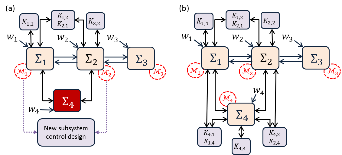
Now consider the networked system $\mathbf{T_{4}}=\mathbf{T_{3}}|\Sigma_{4}$ formed by adding a new subsystem $\Sigma_{4}$ to $\mathbf{T_{3}}$ as shown in Fig. 4(a), where $\Sigma_{4}$ is dynamically coupled to $\Sigma_{1}$ and $\Sigma_{2}$ . The dynamics of $\Sigma_{4}$ is given by

$\displaystyle\Sigma_{4}:\dot{x}_{4}(t)$	$\displaystyle\!=\!\begin{bmatrix}2&1\\ 3&0.8\end{bmatrix}x_{4}(t)\!+\!\begin{bmatrix}1.2\\ 0.8\end{bmatrix}v_{1}(t)\!+\!\begin{bmatrix}0.5\\ -0.2\end{bmatrix}w_{4}(t)\!$
	$\displaystyle\ +\!\begin{bmatrix}1.2\\ 0.8\end{bmatrix}u_{4}(t)$
$\displaystyle y_{4}(t)$	$\displaystyle\!=\!\begin{bmatrix}2.1&0.6\end{bmatrix}x_{4}(t)$	(22)
$\displaystyle v_{4}(t)$	$\displaystyle\!=\!\begin{bmatrix}-0.9&-0.3\end{bmatrix}\!x_{1}(t)\!-\!0.9x_{2}(t)\!+\!\begin{bmatrix}1.1&0.4\end{bmatrix}\!x_{4}(t).$

Additionally, the coupling inputs $v_{1}(t)$ and $v_{2}(t)$ are updated to,

	$\displaystyle v_{1}(t)$	$\displaystyle\!=\!\begin{bmatrix}0.5&-0.7\end{bmatrix}\!x_{1}(t)\!+\!0.1x_{2}(t)\!+\!\begin{bmatrix}0.2&0.2\end{bmatrix}\!x_{4}(t),$
	$\displaystyle v_{2}(t)$	$\displaystyle\!=\!\begin{bmatrix}1&-0.5\end{bmatrix}\!x_{1}(t)\!+\!0.5\!x_{2}(t)\!-\!0.1\!x_{3}(t)\!+\!\begin{bmatrix}0.2&0.2\end{bmatrix}\!x_{4}(t).$

At subsystem $\Sigma_{4}$ , we use matrices $\mathcal{M}_{1}$ , $P_{1}$ , $\mathcal{M}_{2}$ and $P_{2}$ received from $\Sigma_{1}$ and $\Sigma_{2}$ (its neighboring subsystems) in the compositional synthesis procedure described in Algorithm 3 to design controller matrices $K_{4,4}$ , $K_{1,4}$ , $K_{4,1}$ , $K_{4,2}$ and $K_{2,4}$ that guarantee passivity of the networked system $\mathbf{T_{4}}=\mathbf{T_{3}}|\Sigma_{4}$ . The compositional control synthesis procedure is illustrated in Fig. 4. The distributed synthesis algorithm allows for dynamics of subsystems to be dissimilar and of different dimensions, as long as the network is ‘proper’, that is, the input-output dimensions are suitable to define the interconnections between subsystems.

We would like to highlight the fact that the proposed algorithm distributes the analysis and control synthesis between subsystems sequentially. As described in Remark 7, Algorithm 2 is generally always feasible (with only one exception). In the next part of this example, we demonstrate the feasibility of the control synthesis by reapplying the distributed synthesis approach to the same network, but solving the synthesis problem in Algorithm 2 in two different sequences as shown in Fig. 6 and Fig. 8.

Fig. 5: Controller matrices for networked system

\mathbf{T_{4}}

with solution sequence {1-2-3-4}.

V-1 Solution sequence $\{3-2-1-4\}$

Consider the set-up shown in Fig. 6. As opposed to the discussion so far in this example, where the distributed synthesis Algorithm 2 solves $\mathbb{P}_{1}$ (and $\mathbb{P}_{2}$ ) for $\Sigma_{1}$ first, followed by $\Sigma_{2}$ , $\Sigma_{3}$ , and $\Sigma_{4}$ , in that order, we now begin by analyzing $\Sigma_{3}$ first, followed by $\Sigma_{2}$ , $\Sigma_{1}$ , and $\Sigma_{4}$ , in that order. The design steps are summarized below:

(a)

We use the sufficient conditions in Theorem 1 to verify that $\Sigma_{3}$ is passive. Therefore, no controller design is required at $\Sigma_{3}$ , and we set $K_{3,3}=0$ . We also compute and store the messenger and energy matrices $\mathcal{M}_{3}$ and $P_{3}$ respectively of $\Sigma_{3}$ .
(b)

We then consider the network $\mathbf{T}_{2}$ , comprised of the interconnection of $\Sigma_{3}$ and $\Sigma_{2}$ , as shown in Fig. 6-(b). We use the messenger and energy matrices $\mathcal{M}_{3}$ and $P_{3}$ respectively, communicated from $\Sigma_{3}$ , along with the dynamics of $\Sigma_{2}$ in Algorithm 2 to verify the passivity of this network. Since the passivity conditions for $\mathbf{T}_{2}$ are not met, we use Step 10 of Algorithm 2 to synthesize controller matrices $K_{2,2}$ , $K_{2,3}$ , and $K_{3,2}$ at $\Sigma_{2}$ to guarantee passivity of interconnection of $\Sigma_{3}$ and $\Sigma_{2}$ . In this case, the controller matrices $K_{2,3}$ , and $K_{3,2}$ turn out to be zero. We also compute messenger matrix $\mathcal{M}_{2}$ and energy matrix $P_{2}$ at $\Sigma_{2}$ .
(c)

Next, we consider the network $\mathbf{T}_{3}=\mathbf{T}_{2}|\Sigma_{1}$ , as shown in Fig. 6-(c). We use the dynamics of the subsystem $\Sigma_{1}$ , and $\mathcal{M}_{2}$ and $P_{2}$ communicated from $\Sigma_{2}$ to $\Sigma_{1}$ in Algorithm 2 to verify that the network $\mathbf{T}_{3}$ is not passive, that is, problem $\mathbb{P}_{1}$ is infeasible. Therefore, we solve $\mathbb{P}_{2}$ to design controller matrices $K_{1,1}$ , $K_{1,2}$ , and $K_{2,1}$ at $\Sigma_{1}$ to guarantee passivity of the networked system $\mathbf{T_{3}}$ comprised of the interconnection of $\Sigma_{3}$ , $\Sigma_{1}$ and $\Sigma_{2}$ . We also compute messenger matrix $\mathcal{M}_{1}$ and energy matrix $P_{1}$ at $\Sigma_{1}$ .
(d)

Lastly, we apply Algorithm 2 to subsystem $\Sigma_{4}$ . The dynamics of the subsystem $\Sigma_{4}$ , and messenger matrices $\mathcal{M}_{1}$ and $\mathcal{M}_{2}$ , and energy matrices $P_{1}$ and $P_{2}$ , communicated to $\Sigma_{4}$ from its neighboring subsystems $\Sigma_{1}$ and $\Sigma_{2}$ , are used in $\mathbb{P}_{1}$ and $\mathbb{P}_{2}$ to solve for the controller gains $K_{4,4}$ , $K_{4,1}$ , $K_{4,2}$ , $K_{1,4}$ , and $K_{2,4}$ . The closed loop system $\mathbf{T_{4}}$ is guaranteed to be passive.

The designed controller matrices are shown in Fig. 7. Note that although the distributed synthesis algorithm was applied in the sequence $\{3-2-1-4\}$ , the synthesis problem is feasible, and the designed local controllers look very similar to the ones designed when the synthesis algorithm was solved in the sequence $\{1-2-3-4\}$ .

V-2 Solution sequence $\{3-4-1-2\}$

A more interesting scenario is represented in Fig. 8, where the sequence in which Algorithm 8 is applied starts from $\Sigma_{3}$ , and moves on to $\Sigma_{4}$ in the next step, to guarantee passivity of the network $\mathbf{T_{2}}$ comprised of $\Sigma_{3}$ and $\Sigma_{4}$ . Since the two subsystems, $\Sigma_{3}$ and $\Sigma_{4}$ , have no direct coupling, $\mathbf{T}_{2}$ is not fully connected.

Fig. 7: Controller matrices for networked system

\mathbf{T_{4}}

with solution sequence {3-2-1-4}.

However, the results presented in Theorem 1 and Theorem 2 do not impose any restrictions on the topology of the network and can be applied regardless of the connectivity of the graph. Therefore, when the distributed synthesis algorithm is applied to $\Sigma_{4}$ here, it uses the dynamics of $\Sigma_{4}$ in $\mathbb{P}_{1}$ and $\mathbb{P}_{2}$ to compute controller gain $K_{4,4}$ , and messenger matrix $\mathcal{M}_{4}$ and energy matrix $P_{4}$ . The messenger and energy matrices of $\Sigma_{3}$ are not communicated to $\Sigma_{4}$ because $\Sigma_{3}$ and $\Sigma_{4}$ are not coupled. In the next step, $\mathcal{M}_{4}$ and $P_{4}$ are communicated to $\Sigma_{1}$ from $\Sigma_{4}$ and Algorithm 2 is applied to $\Sigma_{1}$ . Note that at this stage, the network $\mathbf{T_{3}}$ comprised of $\Sigma_{1}$ , $\Sigma_{3}$ , and $\Sigma_{4}$ is still not fully connected. However, the proposed distributed synthesis approach still works to guarantee the passivity of the network $\mathbf{T_{3}}$ until this point. Similarly, $\Sigma_{2}$ is added to the network and Algorithm 2 is applied to $\Sigma_{2}$ , using its dynamics, and the messenger and energy matrices, $\mathcal{M}_{1}$ , $\mathcal{M}_{3}$ , $\mathcal{M}_{4}$ , $\mathcal{P}_{1}$ , $\mathcal{P}_{3}$ and $\mathcal{P}_{4}$ , received from its neighbors $\Sigma_{1}$ , $\Sigma_{3}$ and $\Sigma_{4}$ , to guarantee passivity of the networked system $\mathbf{T}_{4}$ . The steps involved in the synthesis are illustrated in Fig. 8, and the designed controller matrices are shown in Fig. 9.

Remark 8

Note that the controller gains designed at $\Sigma_{2}$ using this solution sequence are quite different from the ones designed in Fig. 5 and Fig. 7. This difference can be interpreted in the context of Remark 2 as follows. For the solution sequence $\{1-2-3-4\}$ , when the control design process is

carried out at $\Sigma_{2}$ , the term $\mu_{2}^{c}$ in the messenger matrix $\mathcal{M}_{2}$ corresponding to the energy flow from its neighbors only comprises of the energy flow from subsystem $\Sigma_{1}$ . Similarly, for the solution sequence $\{3-2-1-4\}$ , the messenger matrix $\mathcal{M}_{2}$ only contains the energy flow from the neighbor $\Sigma_{3}$ . However, when the control synthesis algorithm is solved in the sequence $\{3-4-1-2\}$ , the subsystem $\Sigma_{2}$ is added in the last step of the procedure, and the term $\mu_{2}^{c}$ in the messenger matrix $\mathcal{M}_{2}$ comprises of energy flows from all its neighboring subsystems, $\Sigma_{1}$ , $\Sigma_{2}$ , and $\Sigma_{3}$ . This results in large gains for the controllers designed at $\Sigma_{2}$ to ensure the positive definiteness of the messenger matrix $\mathcal{M}_{2}$ . This example highlights the trade-off involved in the proposed distributed synthesis, introduced by the sequential nature of the synthesis algorithm. In achieving distributed synthesis, Algorithm 2 introduces some conservatism, where local controllers may be designed at an intermediate step of the synthesis procedure, even if the networked system as a whole is dissipative. Intuitively, the design of redundant or unnecessary controllers will decrease with the number of subsystems into which the networked system is divided, with a purely centralized synthesis being the least conservative in this regard. However, we note that it is precisely this sequential nature of the synthesis that allows compositionality for networks that may be expanded by adding new subsystems, as described in Section IV-C.

Fig. 9: Controller matrices for networked system

\mathbf{T_{4}}

with solution sequence {3-4-1-2}.


$\displaystyle\mathcal{\overline{M}}_{i}$	$\displaystyle=\begin{cases}\mu^{s}_{1},&i=1\\ \mu^{s}_{i}-\mu^{c}_{i},&i\in\mathbb{N}_{N}\backslash\{1\}\end{cases}$	(27a)
$\displaystyle\hat{H}_{i,j}^{\sigma_{i}}$	$\displaystyle=P_{i}(B_{i}^{(1)^{\sigma_{i}}}H_{i,j}+B_{i}^{(3)^{\sigma_{i}}}K_{i,j}),\hskip 202.00027pti\in\mathbb{N}_{N},\,j\in\mathcal{E}_{i}$	(27b)
$\displaystyle\mu^{s}_{i}$	$\displaystyle=\begin{bmatrix}-(A_{i}^{\sigma_{i}^{\prime}}P_{i}+P_{i}A_{i}^{\sigma_{i}^{\prime}})-(\hat{H}_{i,i}^{\sigma_{i}}+\hat{H}_{i,i}^{\sigma_{i}^{\prime}})+C_{i}^{\sigma_{i}^{\prime}}Q_{i}C_{i}^{\sigma_{i}}&-P_{i}B_{i}^{(2)^{\sigma_{i}}}+C_{i}^{\sigma_{i}^{\prime}}S_{i}\\ -B_{i}^{(2)^{\sigma_{i}^{\prime}}}P_{i}+S^{\prime}_{i}C_{i}^{\sigma_{i}}&R_{i}\end{bmatrix},\hskip 13.00005pti\in\mathbb{N}_{N}$	(27c)
$\displaystyle\mu^{c}_{i}$	$\displaystyle=\sum\limits_{j\in\mathcal{E}_{i}\cap\mathbb{N}_{i-1}}\begin{bmatrix}\hat{H}_{j,i}^{\sigma_{j}^{\prime}}+\hat{H}_{i,j}^{\sigma_{i}}&0\\ 0&0\end{bmatrix}\left(\mathcal{M}_{j}\right)^{-1}\begin{bmatrix}\hat{H}_{j,i}^{\sigma_{j}^{\prime}}+\hat{H}_{i,j}^{\sigma_{i}}&0\\ 0&0\end{bmatrix}^{\prime},\hskip 87.00009pti\in\mathbb{N}_{N}\backslash\{1\}$	(27d)
$\displaystyle\mathcal{M}_{i}$	$\displaystyle=\arg\min\limits_{{\sigma_{i},\sigma_{j}}}\|\|\mathcal{\overline{M}}_{i}\|\|,\hskip 257.00035pti\in\mathbb{N}_{N}$	(27e)

VI Extension to Switched Systems

In many emerging applications of large-scale networked systems in infrastructure networks, the subsystem dynamics, and even the coupling matrices between subsystems can change during operation. For example, in power grids comprised of interconnected microgrids, both the dynamics of individual microgrids and the coupling between microgrids change when a new microgrid is connected to the network, and with changes in the operating point [43]. In order to synthesize local controllers in a distributed manner and guarantee compositionality for such applications, we extend the distributed synthesis presented in Section IV to networks of switched systems, where subsystem dynamics is time-varying.

Consider a networked system $\mathbf{T_{N}^{\sigma}}$ comprised of $N$ subsystems, where the dynamics of the $i$ -th subsystem $\Sigma_{i}$ is switching and is given by

$\displaystyle\dot{x}_{i}(t)$	$\displaystyle=A_{i}^{\sigma_{i}(t)}x_{i}(t)+B_{i}^{(1)^{\sigma_{i}(t)}}v_{i}(t)+B_{i}^{(2)^{\sigma_{i}(t)}}w_{i}(t)$	(23)
	$\displaystyle+B_{i}^{(3)^{\sigma_{i}(t)}}u_{i}(t),$
$\displaystyle y_{i}(t)$	$\displaystyle=C_{i}^{\sigma_{i}(t)}x_{i}(t),$
$\displaystyle v_{i}(t)$	$\displaystyle=\sum\limits_{j\in\mathbb{N}_{N}}H_{i,j}x_{j}(t),$

where $x_{i}(t)$ , $y_{i}(t)$ , $v_{i}(t)$ , $u_{i}(t)$ , and $w_{i}(t)$ are as described in Section III. The system matrices $A_{i}^{\sigma_{i}(t)}$ , $B_{i}^{(1)^{\sigma_{i}(t)}}$ , $B_{i}^{(2)^{\sigma_{i}(t)}}$ , $B_{i}^{(3)^{\sigma_{i}(t)}}$ , and $C_{i}^{\sigma_{i}(t)}$ vary based on the value of the switching signal $\sigma_{i}(t):\mathbb{R}^{+}\to\mathbb{N}_{\eta_{i}}$ , where $\eta_{i}$ is the number of switching modes of $\Sigma_{i}$ . Note that we do not place any restrictions on the sequence in which the dynamics of $\Sigma_{i}$ switches, and do not require the switching sequence to be known a priori.

Now, the dynamics of $\mathbf{T_{N}^{\sigma}}$ is described by

$\displaystyle\dot{x}(t)$	$\displaystyle=A^{\sigma(t)}x(t)+B^{(1)^{\sigma(t)}}v(t)+B^{(2)^{\sigma(t)}}w(t)$	(24)
	$\displaystyle+B^{(3)^{\sigma(t)}}u(t)$
$\displaystyle y(t)$	$\displaystyle=C^{\sigma(t)}x(t)$
$\displaystyle v(t)$	$\displaystyle=Hx(t)$

where

	$\displaystyle A^{\sigma(t)}$	$\displaystyle=\mbox{diag}(A_{1}^{\sigma_{1}(t)},A_{2}^{\sigma_{2}(t)},\dots,A_{N}^{\sigma_{N}(t)})$
	$\displaystyle B^{(j)^{\sigma(t)}}$	$\displaystyle=\mbox{diag}(B_{1}^{(j)^{\sigma_{1}(t)}},B_{2}^{(j)^{\sigma_{2}(t)}},\dots,B_{N}^{(j)^{\sigma_{N}(t)}}),\quad j\in\mathbb{N}_{3}$
	$\displaystyle C^{\sigma(t)}$	$\displaystyle=\mbox{diag}(C_{1}^{\sigma_{1}(t)},C_{2}^{\sigma_{2}(t)},\dots,C_{N}^{\sigma_{N}(t)})$
	$\displaystyle H$	$\displaystyle=\begin{bmatrix}H_{i,j}\end{bmatrix}_{i,j\in\mathbb{N}_{N}}$

and $x(t)$ , $y(t)$ , $v(t)$ , $u(t)$ , $w(t)$ and $\sigma(t)$ are the augmented system state, output, coupling input, control input, disturbance and switching signal formed by stacking $x_{i}(t)$ , $y_{i}(t)$ , $v_{i}(t)$ , $u_{i}(t)$ , $w_{i}(t)$ and $\sigma_{i}(t)$ respectively of all $N$ subsystems.

As described in [44], the classical form of dissipativity in Definition 1 holds for switched system (24) as well. Along the lines of Section IV, we have the following result on distributed synthesis of local controllers to guarantee dissipativity of the networked switched system $\mathbf{T_{N}^{\sigma}}$ .

Theorem 3

The local control inputs

		$\displaystyle u_{i}(t)=\sum\limits_{j\in\mathcal{E}_{i}\cup\{i\}}u_{i,j}(t),\;i\in\mathbb{N}_{N},$		(25)
		$\displaystyle u_{i,j}(t)=K_{i,j}x_{j}(t),\;j\in\mathcal{E}_{i}\cup\{i\},$		(25)

$\displaystyle\mathbb{P}_{4}:\mbox{Find }$	$\displaystyle P_{i},K_{i,i},K_{i,j},K_{j,i}\,j\in\mathcal{E}_{i}$	(26)
$\displaystyle\mbox{s.t.}$	$\displaystyle P_{i}>0,$
	$\displaystyle{\displaystyle\mathcal{\overline{M}}}_{i}>0,$
	$\displaystyle P_{i}\in\mathbb{R}^{n_{i}\times n_{i}},$
	$\displaystyle K_{i,i}\in\mathbb{R}^{p_{i}\times n_{i}},$
	$\displaystyle K_{i,j}\in\mathbb{R}^{p_{i}\times n_{j}},\,K_{j,i}\in\mathbb{R}^{p_{j}\times n_{i}},$

for all $i\in\mathbb{N}_{N}$ and all $\sigma_{i}\in\mathbb{N}_{\eta_{i}}$ , $\sigma_{j}\in\mathbb{N}_{\eta_{j}}$ , $j\in\mathcal{E}_{i}\cap\mathbb{N}_{i-1}$ , where $\mathcal{\overline{M}}_{i}$ is computed from (27), render $\mathbf{T_{N}^{\sigma}}$ (24) $QSR$ -dissipative with

	$\displaystyle Q$	$\displaystyle=\mbox{diag}(Q_{1},Q_{2},\dots,Q_{N}),\quad Q_{i}~\in~\mathbb{R}^{m_{i}\times m_{i}}$
	$\displaystyle S$	$\displaystyle=\mbox{diag}(S_{1},S_{2},\dots,S_{N}),\quad S_{i}\in\mathbb{R}^{m_{i}\times l_{i}}$
	$\displaystyle R$	$\displaystyle=\mbox{diag}(R_{1},R_{2},\dots,R_{N}),\quad R_{i}\in\mathbb{R}^{l_{i}\times l_{i}},\quad i\in\mathbb{N}_{N}.$

The closed-loop messenger matrix of $\Sigma_{i}$ is then given by $\mathcal{M}_{i}=\arg\min\limits_{{\sigma_{i},\sigma_{j}}}||\mathcal{\overline{M}}_{i}||$ .

The messenger matrix $\mathcal{M}_{i}$ in the distributed synthesis result of Theorem 3 corresponds to the least dissipative mode of $\Sigma_{i}$ . This allows for a reduction in the computational complexity of the control synthesis arising from a possibly large number of switching modes in the networked system. If the coupling matrix $H$ is also switching, then the maximum value of the coupling term $\mu_{i,\sigma_{i}}^{c}$ in (27d) over all possible switching sequences of $\Sigma_{j},j\in\mathcal{E}_{i}\cap\mathbb{N}_{i-1}$ can be used in (27a).

Remark 9

Note that Theorem 3 is based on using the same energy matrix $P_{i}$ for all switching modes of $\Sigma_{i}$ in (23). We can allow different energy matrices in different switching modes of the subsystem for specific switching signals that are known a priori. However, it can be shown that a dissipative switched system under arbitrary switching can not have different energy matrices in different switching modes (see Appendix for details).


$\displaystyle A_{i}^{\sigma_{i}}$	$\displaystyle=\begin{bmatrix}-\frac{1}{X_{C,ti}}\left(\sum\limits_{j\in\mathcal{S}_{i,\sigma_{i}}}\frac{X_{R,ij}}{Z_{ij}^{2}}\right)&\omega_{0}-\frac{1}{X_{C,ti}}\left(\sum\limits_{j\in\mathcal{S}_{i,\sigma_{i}}}\frac{\omega_{0}X_{L,ij}}{Z_{ij}^{2}}\right)&\frac{k_{i}}{X_{C,ti}}&0\\ -\omega_{0}+\frac{1}{X_{C,ti}}\left(\sum\limits_{j\in\mathcal{S}_{i,\sigma_{i}}}\frac{\omega_{0}X_{L,ij}}{Z_{ij}^{2}}\right)&-\frac{1}{X_{C,ti}}\left(\sum\limits_{j\in\mathcal{S}_{i,\sigma_{i}}}\frac{X_{R,ij}}{Z_{ij}^{2}}\right)&0&\frac{k_{i}}{X_{C,ti}}\\ -\frac{k_{i}}{X_{L,ti}}&0&\frac{X_{R,ti}}{X_{L,ti}}&\omega_{0}\\ 0&-\frac{k_{i}}{X_{L,ti}}&-\omega_{0}&-\frac{X_{R,ti}}{X_{L,ti}}\end{bmatrix},\quad\begin{matrix}[l]\mathcal{S}_{1,\sigma_{1}}=\begin{cases}\{2\},&\sigma_{1}=1\\ \{2,3\},&\sigma_{1}=2\end{cases}\\ \mathcal{S}_{2,\sigma_{2}}=\{1\},\hskip 26.00009pt\sigma_{2}=1\\ \mathcal{S}_{3,\sigma_{3}}=\{1\},\hskip 26.00009pt\sigma_{3}=1\end{matrix}$	(28a)
$\displaystyle B_{i}^{(1)^{\sigma_{i}}}$	$\displaystyle=\mathbf{I},\quad B_{i}^{(2)^{\sigma_{i}}}=\begin{bmatrix}-\frac{1}{X_{C,ti}}&0&0&0\\ 0&-\frac{1}{X_{C,ti}}&0&0\end{bmatrix}^{\prime},\quad B_{i}^{(3)^{\sigma_{i}}}=\begin{bmatrix}0&0&\frac{1}{X_{L,ti}}&0\\ 0&0&0&\frac{1}{X_{L,ti}}\end{bmatrix}^{\prime}$	(28b)
$\displaystyle C_{i}^{\sigma_{i}}$	$\displaystyle=\mathbf{I},\quad H_{i,j_{1,1}}=\frac{1}{X_{C,ti}}\begin{bmatrix}\frac{X_{R,ij}}{Z_{ij}^{2}}&\frac{\omega_{0}X_{L,ij}}{Z_{ij}^{2}}\\ -\frac{\omega_{0}X_{L,ij}}{Z_{ij}^{2}}&\frac{X_{R,ij}}{Z_{ij}^{2}}\end{bmatrix},\quad H_{i,j}=\left[\begin{array}[]{c;{2pt/2pt}c}H_{i,j_{1,1}}&\\ \hline\cr[2pt/2pt]0&\end{array}\right]$

The compositionality results, as well as the verification and synthesis algorithms in Section IV can similarly be extended to networks of switched systems.

Remark 10 (Extension to nonlinear systems)

In [43], it was shown that the passivity of a nonlinear switched system in a neighborhood around any operating point can be inferred from that of its linear approximation. These results were further extended in [45] to guarantee the dissipativity of a network of nonlinear switched systems through controllers designed in a centralized manner, using the network formed by linear approximations of the nonlinear switched systems. It is easy to see that similar linear approximation arguments can be used to extend the distributed synthesis procedure proposed in this paper to guarantee dissipativity of a networked system comprised of nonlinear subsystems. Additionally, recently developed notions of equilibrium-independent dissipativity (passivity) [46][47] can be explored in the context of guaranteeing dissipativity around non-trivial operating points.

VII Case Study: Microgrid Network

In this section, we consider the problem of compositional synthesis of local controllers for power networks with large-scale integration of renewables. In such networks, several small distributed generation units (DGUs) and loads are aggregated in clusters known as microgrids. In microgrids, since renewable inputs like wind speed and solar intensity vary continuously, and DGUs either participate or do not participate in the network depending on availability and requirement, switching dynamics are inherent [43]. Therefore, it is necessary to synthesize local controllers for DGUs in a compositional manner, such that the stability of the microgrid is maintained when new DGUs connect to the grid, without requiring redesign of existing DGU controllers. In this section, we demonstrate the application of our distributed synthesis framework to enable this ‘plug-and-play’ operation of DGUs in a microgrid.

We consider a microgrid network with three DGUs as shown in Fig. 10. Each DGU is modeled as a voltage source with internal voltage $V_{ti}$ , connected to an RLC-circuit with resistance, inductance and capacitance given by $X_{R,ti}$ , $X_{L,ti}$ and $X_{C,ti}$ respectively. The internal voltage at the DGU is stepped up by a transformer with turn ratio $k_{i}$ to obtain a terminal voltage $V_{i}$ . The line connecting the $i$ -th and $j$ -th DGUs is assumed to have an impedance $Z_{ij}=X_{R,ij}+\sqrt{-1}\omega_{0}X_{L,ij}$ , where $X_{R,ij}$ and $X_{L,ij}$ are the resistance and inductance of the line respectively, and $\omega_{0}$ is the base frequency of the network.

The dynamics of the microgrid can be modeled as a networked switched system, with system matrices given by (28). The system parameters are provided in Table I [48, Appendix C]. As shown in Fig. 10, DGU-3 can either connect or disconnect to DGU-1 in the network. The dynamics of the $i$ -th DGU switches based on the set of DGUs $\mathcal{S}_{i,\sigma_{i}}$ , to which it is connected, as described in (28a). The states (and outputs) of each DGU comprise of the direct and quadrature axis components [49] of the terminal voltages (denoted by $V_{i,d}$ and $V_{i,q}$ respectively) and internal currents at the DGU unit (denoted by $I_{ti,d}$ and $I_{ti,q}$ respectively). The control inputs comprise of the direct and quadrature axis internal voltages of the DGU, denoted by $V_{ti,d}$ and $V_{ti,q}$ respectively. The disturbances correspond to the direct and quadrature axis line currents drawn from the DGU, denoted by $I_{Li,d}$ and $I_{Li,q}$ respectively, which vary based on fluctuations in the power sharing between DGUs.

TABLE I: Parameters of the microgrid network [48]

DGU-1

X_{R,t1}

(

m\Omega

)

1.2

X_{L,t1}

(

\mu H

)

93.7

X_{C,t1}

(

\mu F

)

62.86

DGU-2

X_{R,t2}

(

m\Omega

)

1.6

X_{L,t2}

(

\mu H

)

94.8

X_{C,t2}

(

\mu F

)

62.86

DGU-3

X_{R,t3}

(

m\Omega

)

1.5

X_{L,t3}

(

\mu H

)

107.7

X_{C,t3}

(

\mu F

)

62.86

Line parameters

X_{R,12}

(

\Omega

)

1.1

X_{R,13}

(

\Omega

)

0.9

X_{L,12}

(

mH

)

600

X_{L,13}

(

mH

)

400

Transformer turn ratio

k_{1}=k_{2}=k_{3}

0.0435

Base frequency

\omega_{0}

(

Hz

)

Using Theorem 3, we design local controllers for all DGUs to guarantee $\mathcal{L}_{2}$ stability of the network, by choosing $Q_{i}=-\mathbf{I}$ , $S_{i}=0$ and $R_{i}=\gamma_{i}^{2}\mathbf{I}$ , $i\in\mathbb{N}_{3}$ , where $\gamma_{i}$ represents the $\mathcal{L}_{2}$ gain of the closed loop dynamics of $\Sigma_{i}$ . The parameters $\gamma_{i}$ are considered as variables in the synthesis problem $\mathbb{P}_{2}$ , and are found to be

	$\displaystyle\gamma_{1}$	$\displaystyle=2.85$
	$\displaystyle\gamma_{2}$	$\displaystyle=3.21$
	$\displaystyle\gamma_{3}$	$\displaystyle=3.22.$

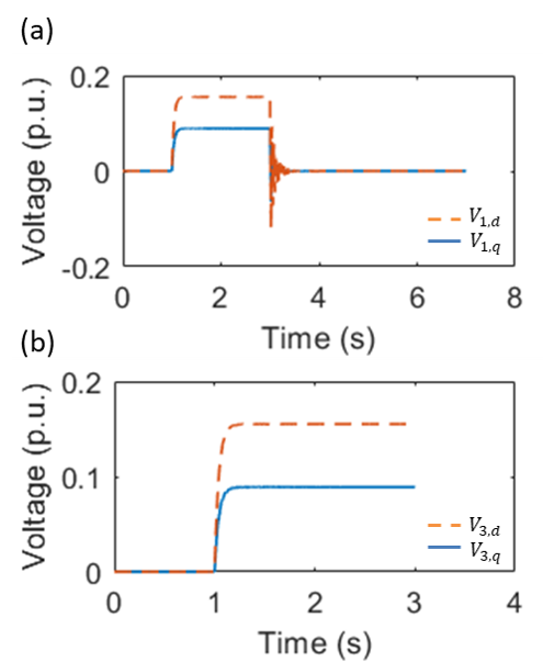
We consider a test scenario where DGU-3 connects to the network at $t=1s$ and disconnects at $t=3s$ , causing a transient in the system states. The terminal voltage profiles (states) at DGU-1 and DGU-3 during this operation are shown in Fig. 11, clearly demonstrating that the proposed controllers maintain the stability of the network during plug-and-play operation.

VIII Conclusion

We presented a distributed and compositional approach to synthesize local controllers for networked systems comprised of dynamically coupled subsystems. The proposed approach can readily be extended to guarantee local dissipativity properties for nonlinear networked systems operating close to equilibrium. Future work will involve extending the distributed synthesis approach to more general classes of nonlinear and hybrid systems.

Proof of Lemma 1
Consider lower triangular matrices ${L}_{i,i},\ i\in\mathbb{N}_{N}$ and matrix

$\displaystyle L$	$\displaystyle=\begin{bmatrix}L_{i,j}\end{bmatrix}_{i,j\in\mathbb{N}_{N}},$	(29)
$\displaystyle L_{i,j}$	$\displaystyle=\begin{cases}0&j>i\\ W_{i,j}L_{j,j}^{\prime-1}&j\in\{2,\ldots,N\},\ j<i\end{cases}$
$\displaystyle L_{i,i}L^{\prime}_{i,i}$	$\displaystyle=\!\begin{cases}\!W_{i,i}&i=1\\ \!W_{i,i}\!-\!\sum\limits_{j\in\mathbb{N}_{i-1}}L_{i,j}L^{\prime}_{i,j}&i\in\{2,\ldots,N\}\end{cases}$

with ${W}_{i,j}$ , $i,j\in\mathbb{N}_{N}$ being elements of $W$ as defined in (7). Define ${M}_{i}=L_{i,i}L^{\prime}_{i,i}$ , $\forall i\in\mathbb{N}_{N}$ .

A symmetric matrix $M_{i}$ is positive definite if and only if there exists a lower triangular matrix $L_{i,i}$ with positive diagonal entries such that $M_{i}=L_{i,i}L^{\prime}_{i,i}$ [50, Section 4]. Therefore, if (8) holds, ${L}_{i,i}$ will exist with positive diagonal entries. Invertibility of $L_{i,i},\,i\in\mathbb{N}_{N}$ guarantees the existence of $L_{i,j},\,i,j\in\mathbb{N}_{N},\,j<i$ . Thus, we can always find a lower triangular matrix $L$ of the form (29), with positive diagonal entries, such that $W=LL^{\prime}$ . This implies the positive definiteness of $W$ [50, Section 4], proving the sufficiency of Lemma 1. Along similar lines, we can also prove the necessity of (9) for the positive definiteness of $W$ . $\blacksquare$

Proof of Theorem 1

From Proposition 1, (2) is $QSR$ -dissipative if

\Gamma=\left[\begin{array}[]{c;{2pt/2pt}c}-\hat{A}^{\prime}P-P\hat{A}+C^{\prime}QC&-PB^{(2)}+C'S\\ \hline\cr[2pt/2pt]-B^{(2)^{\prime}}P+S^{\prime}C&R\end{array}\right]\geq 0,

(30)

where $\hat{A}=A+B^{(1)}H$ . Consider $Q=\mbox{diag}(Q_{1},Q_{2},\dots,Q_{N})$ , $S=\mbox{diag}(S_{1},S_{2},\dots,S_{N})$ , $R=\mbox{diag}(R_{1},R_{2},\dots,R_{N})$ and $P=\mbox{diag}(P_{1},P_{2},\dots,P_{N})$ , where $Q_{i}\in\mathbb{R}^{m_{i}\times m_{i}}$ , $S_{i}\in\mathbb{R}^{m_{i}\times l_{i}}$ , $R_{i}\in\mathbb{R}^{l_{i}\times l_{i}}$ and $P_{i}\in\mathbb{R}^{n_{i}\times n_{i}}$ , $i\in\mathbb{N}_{N}$ . Consider a permutation matrix

\mathbb{E}=\left[\begin{array}[]{cc:cc:c:cc}e_{1}^{\prime}&e_{N+1}^{\prime}\hfil\lx@intercol\vrule\lx@add@cssclass&e_{2}^{\prime}&e_{N+2}^{\prime}\hfil\lx@intercol\vrule\lx@add@cssclass&\cdots\hfil\lx@intercol\vrule\lx@add@cssclass&e_{N}^{\prime}&e_{N+N}^{\prime}\end{array}\right]^{\prime},

where $e_{k},\,k\in\mathbb{R}^{+}\backslash\{0\}$ , are defined as $e_{i}=[e_{i}^{a},0_{n_{i},l}]$ , and $e_{N+i}=[0_{l_{i},n},e_{i}^{b}]$ , where

•

$e_{i}^{a}$ is a matrix with dimension $n_{i}\times n$ , that contains all zero elements, but an identity matrix of dimension $n_{i}$ at columns $(\sum_{j=1}^{i-1}n_{j})+1:(\sum_{j=1}^{i}n_{j})$ .
•

$e_{i}^{b}$ is a matrix with dimension $l_{i}\times l$ , that contains all zero elements, but an identity matrix of dimension $l_{i}$ at columns $(\sum_{j=1}^{i-1}l_{j})+1:(\sum_{j=1}^{i}l_{j})$ .
•

$0_{r,c}$ is a matrix, with $r$ rows and $c$ columns, whose entries are all $0$ .

Right multiplication of $\Gamma$ with $\mathbb{E}^{\prime}$ permutes its columns, and a left multiplication with $\mathbb{E}$ permutes its rows.

$\displaystyle\mathbb{E}\Gamma\mathbb{E}^{\prime}$	$\displaystyle=W=\begin{bmatrix}W_{1,1}&W_{1,2}&\dots&W_{1,N}\\ W_{2,1}&W_{2,2}&\dots&W_{2,N}\\ \vdots&\vdots&&\vdots\\ W_{N,1}&W_{N,2}&\dots&W_{N,N}\\ \end{bmatrix},$	(31)
$\displaystyle W_{i,i}$	$\displaystyle=\left[\begin{array}[]{c;{2pt/2pt}c}-\hat{A}_{i}^{\prime}P_{i}-P_{i}\hat{A}_{i}^{\prime}+C_{i}^{\prime}Q_{i}C_{i}&-P_iB_i^{(2)}+C_i'S_i\\ \hline\cr[2pt/2pt]-B_{i}^{(2)^{\prime}}P_{i}+S_{i}^{\prime}C_{i}&R_i\end{array}\right],$
$\displaystyle W_{i,j}$	$\displaystyle=\left[\begin{array}[]{c;{2pt/2pt}c}-\hat{H}_{i,j}-\hat{H}^{\prime}_{j,i}&\\ \hline\cr[2pt/2pt]0&\end{array}\right],$

for all $i,j\in\mathbb{N}_{N},\ j\neq i$ , where $\hat{A}_{i}=A_{i}+B_{i}^{(1)}H_{i}$ and $\hat{H}_{i,j}=P_{i}B_{i}^{(1)}H_{i,j}$ .

Note that $\Gamma\geq 0$ if and only if $\mathbb{E}\Gamma\mathbb{E}^{\prime}\geq 0$ . If (9) and (10) hold, then, from Lemma 1, $\mathbb{E}\Gamma\mathbb{E}^{\prime}>0$ and all conditions in Proposition 1 are satisfied with $Q=\mbox{diag}(Q_{1},Q_{2},\dots,Q_{N})$ , $S=\mbox{diag}(S_{1},S_{2},\dots,S_{N})$ , $R=\mbox{diag}(R_{1},R_{2},\dots,R_{N})$ and $P=\mbox{diag}(P_{1},P_{2},\dots,P_{N})$ . Therefore, the networked dynamical system $\mathbf{T_{N}}$ in (2) is $QSR$ -dissipative. $\blacksquare$

Proof of Theorem 2

The proof follows by applying Theorem 1 to the closed loop system,

	$\displaystyle\dot{x}_{i}(t)$	$\displaystyle=A_{i}x_{i}(t)+B_{i}^{(1)}v_{i}(t)+B_{i}^{(2)}w_{i}(t)$
		$\displaystyle\ +B_{i}^{(3)}\sum\limits_{j\in\mathcal{E}_{i}}K_{i,j}(t)x_{j}(t),$
	$\displaystyle y_{i}(t)$	$\displaystyle=C_{i}x_{i}(t),$
	$\displaystyle v_{i}(t)$	$\displaystyle=\sum\limits_{j\in\mathbb{N}_{N}}H_{i,j}x_{j}(t).$

$\blacksquare$

Proof of Corollary 1

If $\mathbb{P}_{3}$ is feasible, then Theorem 2 holds for $\mathbf{T_{N+1}}=\mathbf{T_{N}}|\Sigma_{N+1}$ , thus completing the proof. $\blacksquare$

Proof of Theorem 3

Since Definition 1 holds for switched systems [44], along the lines of proof for Theorem 1, the networked switched system (24) with

u_{i}(t)\!=\!\sum\limits_{j\in\mathcal{E}_{i}}\!K_{i,j}x_{j}(t),

$i\in\mathbb{N}_{N}$ , is $QSR$ -dissipative if

\displaystyle W

\displaystyle=\begin{bmatrix}W_{1,1}&W_{1,2}&\dots&W_{1,N}\\ W_{2,1}&W_{2,2}&\dots&W_{2,N}\\ \vdots&\vdots&&\vdots\\ W_{N,1}&W_{N,2}&\dots&W_{N,N}\\ \end{bmatrix}>0

(36)

holds, where

	$\displaystyle W_{i,i}$	$\displaystyle=\left[\begin{array}[]{c;{2pt/2pt}c}-\hat{A}_{i}^{\sigma_{i}^{\prime}}P_{i}-P_{i}\hat{A}_{i}^{\sigma_{i}^{\prime}}\\ +C_{i}^{\sigma_{i}^{\prime}}Q_{i}C_{i}^{\sigma_{i}}&-P_iB_i^{(2)^{\sigma_i}}+C_i^{\sigma_i'}S_i\\ \hline\cr[2pt/2pt]-B_{i}^{(2)^{\sigma_{i}^{\prime}}}P_{i}+S_{i}^{\prime}C_{i}^{\sigma_{i}}&R_i\end{array}\right],$
	$\displaystyle W_{i,j}$	$\displaystyle=\left[\begin{array}[]{c;{2pt/2pt}c}\hat{H}_{j,i}^{\sigma_{j}^{\prime}}+\hat{H}_{i,j}^{\sigma_{i}}&\\ \hline\cr[2pt/2pt]0&\end{array}\right],$

$\hat{A}_{i}^{\sigma_{i}}=A_{i}^{\sigma_{i}}+B_{i}^{(1)^{\sigma_{i}}}H_{i}$ , $\hat{H}_{i,j}^{\sigma_{i}}=P_{i}(B_{i}^{(1)^{\sigma_{i}}}H_{i,j}+B_{i}^{(3)^{\sigma_{i}}}K_{i,j})$ and $i,j~\in~\mathbb{N}_{N},\ j\neq i$ and $\sigma_{i}\in\mathbb{N}_{\eta_{i}}$ . Clearly, if (26) and (27) hold, then, from Lemma 1, the closed loop networked switched system $\mathbf{T_{N}^{\sigma}}$ is $QSR$ -dissipative. $\blacksquare$

Note on Remark 9

Consider a switched system $\Sigma$

	$\displaystyle\dot{x}(t)$	$\displaystyle=A^{\sigma(t)}x(t)+B^{(1)^{\sigma(t)}}v(t)+B^{(2)^{\sigma(t)}}w(t)+B^{(3)^{\sigma(t)}}u(t)$
	$\displaystyle y(t)$	$\displaystyle=C^{\sigma(t)}x(t)$

which switches arbitrarily between two modes $\sigma(t)\in\{1,2\}$ . Suppose $\Sigma$ is $QSR$ -dissipative with multiple energy matrices (or multiple storage functions), that is, if $\sigma(t)=1,\forall t_{0}\leq t\leq t_{1}$ , $\Sigma$ satisfies the dissipativity inequality

\int_{t_{0}}^{t_{1}}\begin{bmatrix}y(\tau)\\ w(\tau)\end{bmatrix}^{\prime}\begin{bmatrix}Q&S\\ S^{\prime}&R\end{bmatrix}\begin{bmatrix}y(\tau)\\ w(\tau)\end{bmatrix}d\tau\geq V_{1}(x(t_{1}))-V_{1}(x(t_{0})),

where $V_{1}(x)=x^{\prime}P_{1}x$ , and if $\sigma(t)=2,\forall t_{0}\leq t\leq t_{1}$ , $\Sigma$ satisfies

\int_{t_{0}}^{t_{1}}\begin{bmatrix}y(\tau)\\ w(\tau)\end{bmatrix}^{\prime}\begin{bmatrix}Q&S\\ S^{\prime}&R\end{bmatrix}\begin{bmatrix}y(\tau)\\ w(\tau)\end{bmatrix}d\tau\geq V_{2}(x(t_{1}))-V_{2}(x(t_{0})),

where $V_{2}(x)=x^{\prime}P_{2}x$ .

If the dynamics of $\Sigma$ switches from mode 1 ( $\sigma=1$ ) to mode 2 ( $\sigma=2$ ) at time $t$ , then, $\sigma(t^{-})=1$ and $\sigma(t^{+})=2$ . Then,

\int_{t^{-}}^{t^{+}}\begin{bmatrix}y(\tau)\\ w(\tau)\end{bmatrix}^{\prime}\begin{bmatrix}Q&S\\ S^{\prime}&R\end{bmatrix}\begin{bmatrix}y(\tau)\\ w(\tau)\end{bmatrix}d\tau\geq V_{2}(x(t))-V_{1}(x(t))

(42)

must hold. Since $\Sigma$ is dissipative for arbitrary switching, consider a different switching signal where $\Sigma$ switches from mode 2 ( $\sigma=2$ ) to mode 1 ( $\sigma=1$ ) at time $t$ . Then,

\int_{t^{-}}^{t^{+}}\begin{bmatrix}y(\tau)\\ w(\tau)\end{bmatrix}^{\prime}\begin{bmatrix}Q&S\\ S^{\prime}&R\end{bmatrix}\begin{bmatrix}y(\tau)\\ w(\tau)\end{bmatrix}d\tau\geq V_{1}(x(t))-V_{2}(x(t)).

(43)

must hold.

Clearly, both (42) and (43) can hold if and only if $V_{1}(x)=V_{2}(x)$ , that is, the energy matrices $P_{1}$ and $P_{2}$ are the same. A similar argument follows for dynamical systems with more than two switching modes. It is therefore not possible to have different energy matrices in different modes for a switched system that is dissipative for arbitrary switching.

References

[1] D. E. Olivares, A. Mehrizi-Sani, A. H. Etemadi, C. A. Cañizares, R. Iravani, M. Kazerani, A. H. Hajimiragha, O. Gomis-Bellmunt, M. Saeedifard, R. Palma-Behnke et al., “Trends in microgrid control,” IEEE Transactions on Smart Grid, vol. 5, no. 4, pp. 1905–1919, 2014.
[2] P. Varaiya, “Smart cars on smart roads: problems of control,” IEEE Transactions on automatic control, vol. 38, no. 2, pp. 195–207, 1993.
[3] S. Sadraddini, S. Sivaranjani, V. Gupta, and C. Belta, “Provably safe cruise control of vehicular platoons,” IEEE Control Systems Letters, vol. 1, no. 2, pp. 262–267, 2017.
[4] G. Antonelli, “Interconnected dynamic systems: An overview on distributed control,” IEEE Control Systems, vol. 33, no. 1, pp. 76–88, 2013.
[5] S.-H. Wang and E. Davison, “On the stabilization of decentralized control systems,” IEEE Transactions on Automatic Control, vol. 18, no. 5, pp. 473–478, 1973.
[6] R. Lau, R. Persiano, and P. Varaiya, “Decentralized information and control: A network flow example,” IEEE Transactions on Automatic Control, vol. 17, no. 4, pp. 466–473, 1972.
[7] M. Aoki, “Some control problems associated with decentralized dynamic systems,” IEEE Transactions on Automatic Control, vol. 16, no. 5, pp. 515–516, 1971.
[8] R. Bellman, “Large systems,” IEEE Transactions on Automatic Control, vol. 19, no. 5, pp. 465–465, 1974.
[9] E. J. Davison and T. N. Chang, “Decentralized stabilization and pole assignment for general proper systems,” IEEE Transactions on Automatic Control, vol. 35, no. 6, pp. 652–664, 1990.
[10] M. Vidyasagar, “Decomposition techniques for large-scale systems with nonadditive interactions: Stability and stabilizability,” IEEE Transactions on Automatic Control, vol. 25, no. 4, pp. 773–779, 1980.
[11] C. Langbort and J.-C. Delvenne, “Distributed design methods for linear quadratic control and their limitations,” IEEE Transactions on Automatic Control, vol. 55, no. 9, pp. 2085–2093, 2010.
[12] F. Farokhi, “Decentralized control of networked systems: Information asymmetries and limitations,” Ph.D. dissertation, KTH Royal Institute of Technology, 2014.
[13] L. Bakule and J. Lunze, “Decentralized design of feedback control for large-scale systems,” Kybernetika, vol. 24, no. 8, pp. 1–3, 1988.
[14] M. E. Sezer and D. Šiljak, “Nested $\varepsilon$ -decompositions and clustering of complex systems,” Automatica, vol. 22, no. 3, pp. 321–331, 1986.
[15] S. Sethi and Q. Zhang, “Near optimization of dynamic systems by decomposition and aggregation,” Journal of Optimization Theory and Applications, vol. 99, no. 1, pp. 1–22, 1998.
[16] S. Sivaranjani, S. Sadraddini, V. Gupta, and C. Belta, “Distributed control policies for localization of large disturbances in urban traffic networks,” in American Control Conference (ACC), 2017. IEEE, 2017, pp. 3542–3547.
[17] S. Sivaranjani, Y.-S. Wang, V. Gupta, and K. Savla, “Localization of disturbances in transportation systems,” in Decision and Control (CDC), 2015 IEEE 54th Annual Conference on. IEEE, 2015, pp. 3439–3444.
[18] C. Langbort, R. S. Chandra, and R. D’Andrea, “Distributed control design for systems interconnected over an arbitrary graph,” IEEE Transactions on Automatic Control, vol. 49, no. 9, pp. 1502–1519, 2004.
[19] C. Conte, N. R. Voellmy, M. N. Zeilinger, M. Morari, and C. N. Jones, “Distributed synthesis and control of constrained linear systems,” in American Control Conference (ACC), 2012. IEEE, 2012, pp. 6017–6022.
[20] M. N. Zeilinger, Y. Pu, S. Riverso, G. Ferrari-Trecate, and C. N. Jones, “Plug and play distributed model predictive control based on distributed invariance and optimization,” in Decision and Control (CDC), 2013 IEEE 52nd Annual Conference on. IEEE, 2013, pp. 5770–5776.
[21] S. Riverso, M. Farina, and G. Ferrari-Trecate, “Plug-and-play model predictive control based on robust control invariant sets,” Automatica, vol. 50, no. 8, pp. 2179–2186, 2014.
[22] M. Cubuktepe, M. Ahmadi, U. Topcu, and B. Hencey, “Compositional analysis of hybrid systems defined over finite alphabets,” IFAC-PapersOnLine, vol. 51, no. 16, pp. 115 – 120, 2018, 6th IFAC Conference on Analysis and Design of Hybrid Systems ADHS 2018.
[23] P. Varutti, B. Kern, and R. Findeisen, “Dissipativity-based distributed nonlinear predictive control for cascaded systems,” IFAC Proceedings Volumes, vol. 45, no. 15, pp. 439–444, 2012.
[24] T. Ishizaki, H. Sasahara, M. Inoue, and J.-i. Imura, “Modularity-in-design of dynamical network systems: Retrofit control approach,” arXiv preprint arXiv:1902.01625, 2019.
[25] S. Xu and J. Bao, “Distributed control of plantwide chemical processes,” Journal of Process Control, vol. 19, no. 10, pp. 1671–1687, 2009.
[26] N. Hudon and J. Bao, “Dissipativity-based decentralized control of interconnected nonlinear chemical processes,” Computers & Chemical Engineering, vol. 45, pp. 84–101, 2012.
[27] X.-L. Tan and M. Ikeda, “Decentralized stabilization for expanding construction of large-scale systems,” IEEE Transactions on Automatic Control, vol. 35, no. 6, pp. 644–651, 1990.
[28] M. J. Tippett and J. Bao, “Dissipativity based distributed control synthesis,” Journal of Process Control, vol. 23, no. 5, pp. 755–766, 2013.
[29] P. Wu and P. J. Antsaklis, “Passivity indices for symmetrically interconnected distributed systems,” in Control & Automation (MED), 2011 19th Mediterranean Conference on. IEEE, 2011, pp. 1–6.
[30] V. Ghanbari, P. Wu, and P. J. Antsaklis, “Large-scale dissipative and passive control systems and the role of star and cyclic symmetries,” IEEE Transactions on Automatic Control, vol. 61, no. 11, pp. 3676–3680, 2016.
[31] M. Arcak, C. Meissen, and A. Packard, Networks of Dissipative Systems: Compositional Certification of Stability, Performance, and Safety. Springer, 2016.
[32] M. Vidyasagar, “New passivity-type criteria for large-scale interconnected systems,” IEEE Transactions on Automatic Control, vol. 24, no. 4, pp. 575–579, 1979.
[33] P. Moylan and D. Hill, “Tests for stability and instability of interconnected systems,” IEEE Transactions on Automatic Control, vol. 24, no. 4, pp. 574–575, 1979.
[34] H. Pota and P. Moylan, “Stability of locally dissipative interconnected systems,” IEEE Transactions on Automatic Control, vol. 38, no. 2, pp. 308–312, 1993.
[35] E. Agarwal, S. Sivaranjani, V. Gupta, and P. Antsaklis, “Sequential synthesis of distributed controllers for cascade interconnected systems,” in American Control Conference, 2019, to appear. [Online]. Available: arXiv:1902.07114
[36] H. Nijmeijer, R. Ortega, A. Ruiz, and A. Van Der Schaft, “On passive systems: from linearity to nonlinearity,” in Nonlinear Control Systems Design 1992. Elsevier, 1993, pp. 373–378.
[37] J. R. Forbes, “Extensions of input-output stability theory and the control of aerospace systems,” Ph.D. dissertation, 2011.
[38] A. Megretski and A. Rantzer, “System analysis via integral quadratic constraints,” IEEE Transactions on Automatic Control, vol. 42, no. 6, pp. 819–830, 1997.
[39] N. Kottenstette, M. J. McCourt, M. Xia, V. Gupta, and P. J. Antsaklis, “On relationships among passivity, positive realness, and dissipativity in linear systems,” Automatica, vol. 50, no. 4, pp. 1003–1016, 2014.
[40] J. G. VanAntwerp and R. D. Braatz, “A tutorial on linear and bilinear matrix inequalities,” Journal of Process Control, vol. 10, no. 4, pp. 363–385, 2000.
[41] C. Langbort, L. Xiao, R. D’Andrea, and S. Boyd, “A decomposition approach to distributed analysis of networked systems,” in 2004 43rd IEEE Conference on Decision and Control (CDC)(IEEE Cat. No. 04CH37601), vol. 4. IEEE, 2004, pp. 3980–3985.
[42] C. Langbort and R. D’Andrea, “Distributed control of heterogeneous systems interconnected over an arbitrary graph,” in 42nd IEEE International Conference on Decision and Control (IEEE Cat. No. 03CH37475), vol. 3. IEEE, 2003, pp. 2835–2840.
[43] E. Agarwal, S. Sivaranjani, and P. J. Antsaklis, “Feedback passivation of nonlinear switched systems using linear approximations,” in Control Conference (ICC), 2017 Indian. IEEE, 2017, pp. 12–17.
[44] J. Zhao and D. J. Hill, “Dissipativity theory for switched systems,” IEEE Transactions on Automatic Control, vol. 53, no. 4, pp. 941–953, 2008.
[45] S. Sivaranjani, E. Agarwal, L. Xie, V. Gupta, and P. Antsaklis, “Mixed voltage angle and frequency droop control for transient stability of interconnected microgrids,” arXiv preprint arXiv:1803.02918, 2018.
[46] G. H. Hines, M. Arcak, and A. K. Packard, “Equilibrium-independent passivity: A new definition and numerical certification,” Automatica, vol. 47, no. 9, pp. 1949–1956, 2011.
[47] J. W. Simpson-Porco, “Equilibrium-independent dissipativity with quadratic supply rates,” IEEE Transactions on Automatic Control, vol. 64, no. 4, pp. 1440–1455, 2018.
[48] S. Riverso, F. Sarzo, and G. Ferrari-Trecate, “Plug-and-play voltage and frequency control of islanded microgrids with meshed topology,” IEEE Transactions on Smart Grid, vol. 6, no. 3, pp. 1176–1184, 2015.
[49] P. M. Anderson and A. A. Fouad, Power system control and stability. John Wiley & Sons, 2008.
[50] G. H. Golub and C. F. Van Loan, Matrix Computations. JHU Press, 2012, vol. 3.

56789141516192021242526273233

Distributed Synthesis of Local Controllers for Networked Systems with Arbitrary Interconnection Topologies

Abstract

Index Terms:

I Introduction

II System Dynamics

III Problem Description

Definition 1

Remark 1

Proposition 1 (Centralized dissipativity analysis)

IV Distributed Synthesis of Local Controllers

IV-A Distributed Analysis

Lemma 1

Theorem 1 (Distributed dissipativity analysis)

Remark 2 (Messenger matrix)

Remark 3

Remark 4

Remark 5 (Robustness to modeling uncertainties)

IV-B Distributed Synthesis

Theorem 2

Remark 6

Remark 7 (Feasibility of distributed synthesis and local performance)

IV-C Compositional Analysis and Control Synthesis

Corollary 1

V Numerical Example

V-1 Solution sequence {3−2−1−4}\{3-2-1-4\}

V-2 Solution sequence {3−4−1−2}\{3-4-1-2\}

Remark 8

VI Extension to Switched Systems

Theorem 3

Remark 9

Remark 10 (Extension to nonlinear systems)

VII Case Study: Microgrid Network

VIII Conclusion

References

V-1 Solution sequence $\{3-2-1-4\}$

V-2 Solution sequence $\{3-4-1-2\}$