Backscatter Data Collection with Unmanned Ground Vehicle: Mobility Management
and Power Allocation

We consider a wireless data collection system, which consists of $K$ IoT users and one UGV equipped with a RF transmitter and a tag reader. The environment in which the UGV operates in is described by a directed graph $(\mathcal{V},\mathcal{E})$ as shown in Fig. 1, where $\mathcal{V}=\{1,\cdots,M\}$ is the set of $M$ vertices representing the possible stopping points, and $\mathcal{E}$ is the set of directed edges representing the allowed movement paths [24]. To quantify the path length, a matrix $\mathbf{D}=[D_{1,1},\cdots,D_{1,M};\cdots;D_{M,1},\cdots,D_{M,M}]\in\mathbb{R}^{M\times M}_{+}$ is defined, with the element $D_{m,j}$ representing the distance from vertex $m$ to vertex $j$ ($D_{m,m}=0$ for any $m$). If there is no allowed path from vertex $m$ to vertex $j$, we set $D_{m,j}=+\infty$ [24]. Notice that $\mathbf{D}$ is a constant matrix since the locations of all vertices are pre-determined.

To model the movement of the UGV, we define a visiting path $\mathcal{Q}=(y_{1},y_{2},\cdots,y_{Q})$ where $y_{j}\in\mathcal{V}$ for $j=1,\cdots,Q$ and $(y_{j},y_{j+1})\in\mathcal{E}$ for $j=1,\cdots,Q-1$, with $Q-1$ being the number of steps to be taken. Without loss of generality, we assume the following two conditions hold:

• (i)

  $y_{1}=y_{Q}$. This is generally true as a typical UGV management scenario is to have the UGV standing by at the starting point (e.g., for charging and maintenance services) after the data collection task [16]. For notational simplicity, it is assumed that vertex $y_{1}=y_{Q}=1$ is the start and end point of the path to be designed.

• (ii)

  There are no repeating vertices among $(y_{1},\cdots,y_{Q-1})$. This is true because if a vertex $m$ is visited twice, we can always introduce an auxiliary vertex with $D_{M+1,j}=D_{m,j}$ and $D_{j,M+1}=D_{j,m}$ for all $j\in\mathcal{V}$ [16, 25]. Thus this scenario can be represented by an extended graph with one more vertex and an extended $\mathbf{D}$ with dimension $(M+1)\times(M+1)$.

Correspondingly, we define the selection variable $\mathbf{v}=[v_{1},\cdots,v_{M}]^{T}\in\{0,1\}^{M}$, where $v_{m}=1$ if the vertex $m$ appears in the path $\mathcal{Q}$ and $v_{m}=0$ otherwise. Furthermore, we define a matrix $\mathbf{W}=[W_{1,1},\cdots,W_{1,M};\cdots;W_{M,1},\cdots,W_{M,M}]\in\{0,1\}^{M\times M}$, with $W_{y_{j},y_{j+1}}=1$ for all $j=1,\cdots,Q-1$ and zero otherwise.

With the moving time from the vertex $m$ to the vertex $j$ being $D_{m,j}/a$ where $a$ is the velocity, the total moving time along path $\mathcal{Q}$ is

Furthermore, since the total motion energy $E$ of the UGV is proportional to the total motion time [11, 12, 13], the motion energy can be expressed in the form of

where $\alpha_{1}$ and $\alpha_{2}$ are parameters of the model (e.g., for a Pioneer 3DX robot in Fig. 1, $\alpha_{1}=0.29$ and $\alpha_{2}=7.4$ [11, Sec. IV-C]).

Based on the mobility model, the UGV moves along the selected path $\mathcal{Q}$ to collect data from users as shown in Fig. 2. In particular, from the starting point $y_{1}$, the UGV stops for a duration $u_{y_{1}}$ and then it moves along edge $(y_{1},y_{2})$ to its outward neighbor $y_{2}$, and stops for a duration $u_{y_{2}}$. The UGV keeps on moving and stopping along the path until it reaches the destination $y_{Q}$.

When the UGV stops at the vertex $m$ (with $v_{m}=1$), it will wait for a time duration $u_{m}$ for data collection. Out of this $u_{m}$, a duration of $t_{k,m}$ will be assigned to collect data from user $k$ via full-duplex backscatter communication¹¹ 1 When user $k$ adapts the variable impedance for modulating the backscattered waveform with information bits, other users keep silent to avoid collision [6]. [26, 27]. More specifically, if $t_{k,m}=0$, the IoT user $k$ will not be served in duration $u_{m}$. On the other hand, if $t_{k,m}\neq 0$, the RF source at the UGV transmits a symbol $x_{k,m}\in\mathbb{C}$ with $\mathbb{E}[|x_{k,m}|^{2}]=p_{k,m}$, where $p_{k,m}$ is the transmit power of the RF source. Then the received signal-to-noise ratio (SNR) at the UGV tag reader is $\eta|g_{k,m}|^{2}|h_{k,m}|^{2}p_{k,m}/N_{0}$, where $h_{k,m}\in\mathbb{C}$ is the downlink channel from the UGV to user $k$, $g_{k,m}\in\mathbb{C}$ is the uplink channel from user $k$ to the UGV, and $N_{0}$ is the power of complex Gaussian noise (including the self-interference due to full-duplex backscatter [26, 27]). Furthermore, $\eta$ is the tag scattering efficiency determined by the load impedance $Z_{L}$ and the antenna impedance $Z_{A}$ [28]. For example, in the on-off keying backscatter shown in Fig. 2, the IoT device switches between two load impedances $Z_{1}$ and $Z_{2}$ with $Z_{1}\neq Z_{A}$ and $Z_{2}=Z_{A}$. This means that the IoT device transmits $(Z_{L}-Z_{A})/(Z_{L}+Z_{A})=(Z_{1}-Z_{A})/(Z_{1}+Z_{A})$ when switching to $Z_{L}=Z_{1}$ and transmits $(Z_{L}-Z_{A})/(Z_{L}+Z_{A})=0$ when switching to $Z_{L}=Z_{2}$. Therefore, $\eta=|(Z_{1}-Z_{A})/(Z_{1}+Z_{A})|^{2}$ in the on-off keying.

Based on the backscatter model, the transmission rate during $t_{k,m}$ is given by

where $\beta$ is the performance loss due to imperfect modulation and coding schemes in backscatter communication [29]. For example, in bistatic backscatter communication with frequency shift keying, $\beta=0.5$ [29]. On the other hand, in ambient backscatter communication with on-off keying, $\beta$ is obtained by fitting $\mathrm{log}_{2}\left(1+\beta x\right)$ to $1-\mathbb{Q}\left(\sqrt{x}\right)$ [30], where $\mathbb{Q}\left(x\right)=1/\sqrt{2\pi}\int_{x}^{\infty}\mathrm{exp}\left(-u^{2}/2\right)\mathrm{d}u$ refers to the Q-function.

Remark 1: The channels $\{g_{k,m},h_{k,m}\}$ can be pre-determined as follows. If the environment is static, all the information about object positions, geometry and dielectric properties in the environment is available. In such a case, ray tracing methods [31] could be used to estimate $\{g_{k,m},h_{k,m}\}$. On the other hand, if the channel is varying but with a fixed distribution, we could allow the UGV to collect a small number of measurements at the stopping points before a set of new missions (e.g., five missions) [32]. Then based on the probabilistic framework in [32], the UGV can predict the channels at all the stopping points.

Remark 2: In practice, the backscatter efficiency would vary with the incident power. However, if the change of backscatter efficiency is not significant, it is possible to adopt a constant $\eta$ to facilitate the analysis [8, 9, 29, 33]. On the other hand, if $\eta$ is not a constant, according to [34], it is possible to compute the range of $\eta$. Then, the worst case approach, which replaces $\eta$ in (3) with its lower bound $\eta_{\mathrm{lb}}$, can be adopted to guarantee the data collection targets for all users. Notice that this worst case approach can only achieve suboptimal performance, and modeling $\eta$ as a nonlinear function of the incident power is an important future work.

To address the challenges for solving $\mathrm{P}1$, we first establish the optimality condition of $\mathrm{P}1$. In particular, by defining

the following proposition (proved in Appendix A) can be established.

Proposition 1 indicates that the UGV only needs to allocate time to user $k$ at a single vertex, which is given by $m=\mathrm{argmax}_{l\in\mathcal{V}}~v^{*}_{l}A_{k,l}$. For other vertices, the allocated time to user $k$ should be zero. Based on part (i) of Proposition 1, we can set the transmit time

where $s_{k}>0$, without changing the optimal solution to $\mathrm{P}1$. Correspondingly, the transmit power $\{p_{k,m}\}$ can be set to³³ 3 If $m\neq\mathop{\mathrm{argmax}}_{l\in\mathcal{V}}~v_{l}A_{k,l}$, we have $t_{k,m}=0$. Thus $t_{k,m}p_{k,m}=0$ in the objective of $\mathrm{P}1$ and $t_{k,m}\mathrm{log}_{2}\left(1+v_{m}A_{k,m}p_{k,m}\right)=0$ in (7a), meaning that $p_{k,m}$ would not participate in problem $\mathrm{P}1$. As a result, we can set $p_{k,m}=0$.

where $q_{k}$ is the transmit power corresponding to $s_{k}$. Since $s_{k}>0$, by part (ii) of Proposition 1, we also have $q_{k}>0$. Putting (9) and (10) into $\mathrm{P}1$, problem $\mathrm{P}1$ is transformed into

Notice that the constraint (7h) is dropped since (7h) is always satisfied when $\{t_{k,m}\}$ takes the form of (9).

The problem $\mathrm{P}2$ is still nontrivial to solve due to the nonlinear coupling between $\mathbf{v}$ and $\{\mathbf{W},s_{k},q_{k}\}$ as observed from the constraints (11a) and (11c). To resolve such coupling, a straightforward idea is to use alternating minimization for optimizing $\mathbf{v}$, $\mathbf{W}$ and $\{s_{k},q_{k}\}$ iteratively. However, due to the discrete nature of $\mathbf{v}$ and $\mathbf{W}$, such a method could fail to converge. To this end, this paper proposes to simplify the problem based on elimination of variables. In particular, we will first derive the optimal solution of $\mathbf{W}$ and $\{s_{k},q_{k}\}$ to $\mathrm{P}2$ with fixed $\mathbf{v}$. By representing $\mathbf{W}$ and $\{s_{k},q_{k}\}$ as functions of $\mathbf{v}$, problem $\mathrm{P}2$ is simplified to an equivalent problem only involving $\mathbf{v}$. Then we will step further to find the optimal solution of vertex selection variable $\mathbf{v}$.

When $\mathbf{v}=\widetilde{\mathbf{v}}$, where $\widetilde{\mathbf{v}}$ is any feasible solution to $\mathrm{P}2$, the constraint (7g) can be dropped since it only involves $\mathbf{v}$. On the other hand, the term $\mathop{\mathrm{max}}_{l\in\mathcal{V}}~\widetilde{v}_{l}A_{k,l}$ in constraint (11a) becomes a constant, and we denote it as $B_{k}(\widetilde{\mathbf{v}}):=\mathop{\mathrm{max}}_{l}~\widetilde{v}_{l}A_{k,l}$. Furthermore, it can be seen from the objective function of $\mathrm{P}2$ that $q_{k}$ is a variable to be minimized and $s_{k}\mathrm{log}_{2}\left[1+B_{k}(\widetilde{\mathbf{v}})q_{k}\right]$ is a strictly increasing function of $q_{k}$. As a result, the optimal solution of $q_{k}$ must activate the constraint (11a) of $\mathrm{P}2$, which leads to

Putting (12) into $\mathrm{P}2$, it is proved in Appendix B that the optimal $\mathbf{W}^{*}$ and $\{s_{k}^{*}\}$ to $\mathrm{P}2$ must activate the constraint (11b), i.e., $\mathrm{Tr}(\mathbf{D}^{T}\mathbf{W}^{*})/a+\sum_{k=1}^{K}s_{k}^{*}=T$. Using this result, the quantity $\mathrm{Tr}(\mathbf{D}^{T}\mathbf{W})$ in the objective function of $\mathrm{P}2$ can be replaced by $a(T-\sum_{k=1}^{K}s_{k})$ without changing the problem, and the objective function would be independent of $\mathbf{W}$. Then problem $\mathrm{P}2$ is equivalently transformed into the following two-stage optimization problem (detailed procedure given in Appendix B):

where $\Theta(x):=x(2^{1/x}-1)$.

To solve $\mathrm{P}3$, we first need to compute the right hand side of the constraint, which leads to the following problem:

The problem (13) is a travelling salesman problem, which can be optimally solved by the one-tree relaxation algorithm via the software Mosek [25]. In particular, the one-tree relaxation algorithm is an iterative procedure that finds a sequence of one-tree upper bounds to the problem (13) until convergence [25], and the converged solution is guaranteed to be optimal.

Denoting the optimal solution to the problem (13) as $\{\widehat{\mathbf{W}},\widehat{\lambda}_{m}\}$, the optimal objective value of the travelling salesman problem is given by

Now, by putting the obtained $\Upsilon(\widetilde{\mathbf{v}})$ into $\mathrm{P}3$, the constraint of $\mathrm{P}3$ is written as $\sum_{k=1}^{K}s_{k}=\Upsilon(\widetilde{\mathbf{v}})$. Assigning a Lagrange multiplier $\rho$ to this constraint, the Lagrangian of $\mathrm{P}3$ is

According to the first-order KKT condition $\frac{\partial\mathcal{L}}{\partial s_{k}}|_{s_{k}=\widehat{s}_{k}}=0$, the optimal $\{\widehat{s}_{k}\}$ and $\widehat{\rho}$ should together satisfy [41]:

where $-\nabla\Theta(x)$ is the gradient of $-\Theta(x)$ and is given by

with $x>0$. Moreover, as $-\nabla^{2}\Theta(x)=-\mathrm{ln}^{2}2\cdot 2^{1/x}/x^{3}<0$ and $-\nabla^{3}\Theta(x)=\mathrm{ln}^{3}2\cdot 2^{1/x}/x^{5}+3\mathrm{ln}^{2}2\cdot 2^{1/x}/x^{4}>0$, it can be seen that $-\nabla\Theta(x)$ is a strictly decreasing and convex function of $x$. As a result, there must exist a strictly decreasing and convex function $\Lambda(x)$ such that $\Lambda(-\nabla\Theta(x))=x$. That is, the function $\Lambda(x)$ is the inverse function of $-\nabla\Theta(x)$, and it can be numerically computed and stored as a look-up table, with its shape shown in Fig. 3. Applying $\Lambda(x)$ to both sides of (15), we have

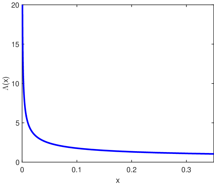
Notice that in (17), the only unknown is $\widehat{\rho}$, which should satisfy the equality constraint of $\mathrm{P}3$:

Since $\Lambda(x)$ is a decreasing function, bisection search method can be used to find $\widehat{\rho}$ efficiently. In order to determine the bisection interval, the following proposition (proved in Appendix C) can be established.

Once $\widehat{\rho}$ is obtained, we can put $\widehat{\rho}$ into (17) to get $\{\widehat{s}_{k}\}$. Further putting $\{\widehat{s}_{k}\}$ into (12), we have $\widehat{q}_{k}=\left(2^{\gamma_{k}/\widehat{s}_{k}}-1\right)\Big/B_{k}(\widetilde{\mathbf{v}})$.

With path $\widehat{\mathbf{W}}$, transmit times $\{\widehat{s}_{k}\}$, and transmit powers $\{\widehat{q}_{k}\}$ derived in Section IV-B, the optimal objective value of $\mathrm{P}3$ (equivalently $\mathrm{P}2$ with $\mathbf{v}=\widetilde{\mathbf{v}}$) is given by

Therefore, problem $\mathrm{P}2$ is re-written as

To solve $\mathrm{P}4$, a naive way is to apply exhaustive search for $\mathbf{v}$. Unfortunately, since the searching space of $\{v_{m}\}$ is very large (i.e., $2^{M-1}$), direct implementation of exhaustive search is impossible. To address the above issue, a B$\&$B method is presented for systematically pruning out impossible solutions of $\mathbf{v}$, leading to significant reduction of the computational complexity compared to exhaustive search while guaranteeing the global optimality [42, 43].

In particular, we define the living pool as a set $\mathcal{Y}$ which stores all the solutions that have not been explored, and the incumbent $I$ as the current best objective value that has been obtained. Initially, $I$ can be set to the objective value of any feasible solution. On the other hand, since the feasible set of $\mathbf{v}$ for $\mathrm{P}4$ is $\Omega=\left\{\mathbf{v}\in\{0,1\}^{M}:v_{1}=1\right\}$, the initial living pool can be set to $\mathcal{Y}=\{\mathcal{F}_{(1,0)},\mathcal{F}_{(1,1)}\}$ (notice that $\mathcal{Y}$ is a family of sets over $\Omega$), where $\mathcal{F}_{(1,0)}=\left\{\mathbf{v}\in\Omega:v_{2}=0\right\}$ and $\mathcal{F}_{(1,1)}=\left\{\mathbf{v}\in\Omega:v_{2}=1\right\}$ as shown in Fig. 4a. It can be seen that $\Omega=\mathcal{F}_{(1,0)}\bigcup\mathcal{F}_{(1,1)}$ and $\mathcal{F}_{(1,0)},\mathcal{F}_{(1,1)}\subset\Omega$.

At the beginning, the B$\&$B method computes a lower bound $\Psi(\mathcal{F}_{(1,0)})$ such that $\Psi(\mathcal{F}_{(1,0)})\leq\Xi(\widetilde{\mathbf{v}})$ for any $\widetilde{\mathbf{v}}\in\mathcal{F}_{(1,0)}$, where $\Xi(\widetilde{\mathbf{v}})$ is defined in (IV-C). Based on the bounding function value $\Psi(\mathcal{F}_{(1,0)})$, we consider the following three cases.

• (i)

  If $\Psi(\mathcal{F}_{(1,0)})>I$, then the subset $\mathcal{F}_{(1,0)}$ can be discarded, since no feasible solution inside $\mathcal{F}_{(1,0)}$ leads to better objective than the incumbent. Therefore, we update $\mathcal{Y}\leftarrow\mathcal{Y}\setminus\mathcal{F}_{(1,0)}$. This case is shown in Fig. 4b.

• (ii)

  If $\Psi(\mathcal{F}_{(1,0)})\leq I$ and $|\mathcal{F}_{(1,0)}|>1$, the possibility of a better solution in $\mathcal{F}_{(1,0)}$ cannot be ruled out. As a result, we need to branch on $\mathcal{F}_{(1,0)}$ and generates two subsets $\mathcal{F}_{(1,0,0)}=\left\{\mathbf{v}\in\mathcal{F}_{(1,0)}:v_{3}=0\right\}$ and $\mathcal{F}_{(1,0,1)}=\left\{\mathbf{v}\in\mathcal{F}_{(1,0)}:v_{3}=1\right\}$. By treating $\mathcal{F}_{(1,0,0)}$ and $\mathcal{F}_{(1,0,1)}$ as new subset nodes, we update $\mathcal{Y}\leftarrow\mathcal{Y}\setminus\mathcal{F}_{(1,0)}\cup\{\mathcal{F}_{(1,0,0)},\mathcal{F}_{(1,0,1)}\}$. This case is shown in Fig. 4c.

• (iii)

  Otherwise, we must have $|\mathcal{F}_{(1,0)}|=1$. Denoting the unique element in $|\mathcal{F}_{(1,0)}|$ as $\widetilde{\mathbf{v}}$, we compute $\Xi(\widetilde{\mathbf{v}})$. If $\Xi(\widetilde{\mathbf{v}})>I$, $\mathcal{F}_{(1,0)}$ is discarded. On the other hand, if $\Xi(\widetilde{\mathbf{v}})\leq I$, the incumbent is updated as $I\leftarrow\Xi(\widetilde{\mathbf{v}})$ and the current best solution is updated as $\mathbf{v}^{\diamond}\leftarrow\widetilde{\mathbf{v}}$. In both cases, since there is no more element in $\mathcal{F}_{(1,0)}$ to be evaluated, we can update $\mathcal{Y}\leftarrow\mathcal{Y}\setminus\mathcal{F}_{(1,0)}$.

After $\mathcal{F}_{(1,0)}$ is evaluated, we then evaluate $\mathcal{F}_{(1,1)},\mathcal{F}_{(1,0,0)},\mathcal{F}_{(1,0,1)},\cdots$ by repeating the above procedure until the living pool $\mathcal{Y}$ becomes empty.

For the above B$\&$B method, the key step is to derive the bounding function $\Psi$. In particular, to guarantee that the proposed B$\&$B method finds the optimal solution of $\mathbf{v}$ to $\mathrm{P}4$, the bounding function needs to satisfy [42]:

where $(z_{1},\cdots,z_{N})$ are the values assigned to $(v_{1},\cdots,v_{N})$ and $N$ is the number of fixed elements in $\mathbf{v}$. To this end, consider the following bounding function $\Psi$:

where $\mathbf{z}=[z_{1},\cdots,z_{N}]^{T}\in\{0,1\}^{N}$ (corresponding to the sequence $(z_{1},\cdots,z_{N})$), and $\delta$ is the solution to

The function

References

- [1] J. Chen, K. Hu, Q. Wang, Y. Sun, Z. Shi, and S. He, “Narrowband Internet of Things: Implementations and applications,” IEEE IoT Journal, vol. 4, no. 6, pp. 2309-2314, Dec. 2017.
- [2] M. Xia and S. Aïssa, “On the efficiency of far-field wireless power transfer,” IEEE Trans. Signal Process., vol. 63, no. 11, pp. 2835-2847, Jun. 2015.
- [3] V. Liu, A. Parks, V. Talla, S. Gollakota, D. Wetherall, and J. R. Smith, “Ambient backscatter: Wireless communication out of thin air,” in Proc. ACM SIGCOMM, 2013, pp. 39-50.
- [4] J. Kimionis, A. Bletsas, and J. N. Sahalos, “Increased range bistatic scatter radio,” IEEE Trans. Commun., vol. 62, no. 3, pp. 1091-1104, Mar. 2014.
- [5] C. Boyer and S. Roy, “Backscatter communication and RFID: Coding, energy, and MIMO analysis,” IEEE Trans. Commun., vol. 62, no. 3, pp. 770-785, Mar. 2014.
- [6] A. Alma’aitah, H. S. Hassanein, and M. Ibnkahla, “Tag modulation silencing: Design and application in RFID anti-collision protocols,” IEEE Trans. Commun., vol. 62, no. 11, pp. 4068-4079, Nov. 2014
- [7] B. Clerckx, Z. B. Zawawi, and K. Huang, “Wirelessly powered backscatter communications: Waveform design and SNR-energy tradeoff,” IEEE Commun. Lett., vol. 21, no. 10, pp. 2234-2237, Oct. 2017.
- [8] B. Lyu, H. Guo, Z. Yang, and G. Gui, “Throughput maximization for hybrid backscatter assisted cognitive wireless powered radio networks,” IEEE IoT Journal, vol. 5 , no. 3, pp. 2015-2024, Jun. 2018.
- [9] G. Wang, F. Gao, R. Fan, and C. Tellambura, “Ambient backscatter communication systems: Detection and performance analysis,” IEEE Trans. Commun, vol. 64, no. 11, pp. 4836-4846, Nov. 2016.
- [10] J. Qian, F. Gao, G. Wang, S. Jin, and H. Zhu, “Noncoherent detections for ambient backscatter systems,” IEEE Trans. Wireless Commun., vol. 16, no. 3, pp. 1412-1422, Mar. 2017.
- [11] Y. Mei, Y. H. Lu, Y. Hu, and C. Lee, “Deployment of mobile robots with energy and timing constraints,” IEEE Trans. Robotics, vol. 22, no. 3, pp. 507-522, Jun. 2006.
- [12] G. Wang, M. J. Irwin, P. Berman, H. Fu, and T. F. L. Porta, “Optimizing sensor movement planning for energy efficiency,” in Proc. ISLPED, pp. 215-220, 2005.
- [13] Y. Yan and Y. Mostofi, “Co-optimization of communication and motion planning of a robotic operation under resource constraints and in fading environments,” IEEE Trans. Wireless Commun., vol. 12, no. 4, pp. 1562-1572, Apr. 2013.
- [14] Y. Shu, H. Yousefi, P. Cheng, J. Chen, Y. Gu, T. He, and K. G. Shin, “Near-optimal velocity control for mobile charging in wireless rechargeable sensor networks,” IEEE Trans. Mobile Comput., vol. 15, no. 7, pp. 1699-1713, Jul. 2016.
- [15] S. Wang, M. Xia, K. Huang, and Y.-C. Wu, “Wirelessly powered two-way communication with nonlinear energy harvesting model: Rate regions under fixed and mobile relay,” IEEE Trans. Wireless Commun., vol. 16, no. 12, pp. 8190 -8204, Dec. 2017.
- [16] G. Laporte, “The vehicle routing problem: An overview of exact and approximate algorithms,” European Journal of Operational Research, vol. 59, no. 3, pp. 345-358, 1992.
- [17] M. Ma, Y. Yang, and M. Zhao, “Tour planning for mobile data gathering mechanisms in wireless sensor networks,” IEEE Trans. Veh. Technol., vol. 62, no. 4, pp. 1472-1483, May 2013.
- [18] M. Zhao, J. Li, and Y. Yang, “A framework of joint mobile energy replenishment and data gathering in wireless rechargeable sensor networks,” IEEE Trans. Mobile Comput., vol. 13, no. 12, pp. 2689-2705, Dec. 2014.
- [19] Y. Zeng and R. Zhang, “Energy-efficient UAV communication with trajectory optimization,” IEEE Trans. Wireless Commun., vol. 16, no. 6, pp. 3747-3760, Jun. 2017.
- [20] Q. Wu, Y. Zeng, and R. Zhang, “Joint trajectory and communication design for multi-UAV enabled wireless networks,” IEEE Trans Wireless Commun., vol. 17, no. 3, pp. 2109-2121, Mar. 2018.
- [21] Y Sun, D. W. K. Ng, D. Xu, L. Dai, and R. Schober, “Resource allocation for solar powered UAV communication systems,” in Proc. IEEE SPAWC’18, Kalamata, Greece, Jun. 2018.
- [22] H. Sallouha, M. M. Azari, and S. Pollin, “Energy-constrained UAV trajectory design for ground node localization,” in Proc. IEEE GLOBECOM, Abu Dhabi, UAE, Dec. 2018.
- [23] H. Sallouha, M. M. Azari, A. Chiumento, and S. Pollin, “Aerial anchors positioning for reliable rss-based outdoor localization in urban environments,” IEEE Wireless Commun. Lett., vol. 7, no. 3, pp. 376-379, Jun. 2018.
- [24] J. A. Bondy and U. Murthy, Graph Theory with Applications. New York: Elsevier, 1976.
- [25] G. Laporte, “The traveling salesman problem: An overview of exact and approximate algorithms,” European Journal of Operational Research, vol. 59, no. 2, pp. 231-247, 1992.
- [26] V. Liu, V. Talla, and S. Gollakota, “Enabling instantaneous feedback with full-duplex backscatter,” in Proc. ACM MobiCom, 2014, pp. 67-78.
- [27] W. Liu, K. Huang, X. Zhou, and S. Durrani, “Full-duplex backscatter interference networks based on time-hopping spread spectrum,” IEEE Trans. Wireless Commun., vol. 16, no. 7, pp. 4361-4377, Jul. 2017.
- [28] G. Zhu, S. W. Ko, and K. Huang, “Inference from randomized transmissions by many backscatter sensors,” IEEE Trans. Wireless Commun., vol. 17, no. 5, pp. 3111-3127, May 2018.
- [29] S. H. Kim and D. I. Kim, “Hybrid backscatter communication for wireless-powered heterogeneous networks,” IEEE Trans. Wireless Commun., vol. 16, no. 10, pp. 6557-6570, Oct. 2017.
- [30] J. G. Proakis, Digital Communications (4th edition). New York, NY, USA: McGraw-Hill, 2001.
- [31] K. A. Remley, H. R. Anderson, and A. Weisshar, “Improving the accuracy of ray-tracing techniques for indoor propagation modeling,” IEEE Trans. Veh. Technol., vol. 49, no. 6, pp. 2350-2358, Nov. 2000.
- [32] M. Malmirchegini and Y. Mostofi, “On the spatial predictability of communication channels,” IEEE Trans. Wireless Commun., vol. 11, no. 3, pp. 964-978, Mar. 2012.
- [33] P. N. Alevizos, K. Tountas, and A. Bletsas, “Multistatic scatter radio sensor networks for extended coverage,” IEEE Trans. Wireless Commun., vol. 17, no. 7, pp. 4522-4535, Jul. 2018.
- [34] A. Bletsas, A. G. Dimitriou, and J. N. Sahalos, “Improving Backscatter Radio Tag Efficiency,” IEEE Trans. Microw. Theory Techn., vol. 58, no. 6, pp. 1502-1509, Jun. 2010.
- [35] S. Claessens, D. Schreurs, and S. Pollin, “SWIPT with biased ASK modulation and dual-purpose hardware,” in Proc. WPTC, Taipei, May 2017.
- [36] S. Claessens, N. Pan, M. Rajabi, D. Schreurs, and S. Pollin, “Enhanced biased ASK modulation performance for SWIPT with AWGN channel and dual-purpose hardware,” IEEE Trans. Microw. Theory Techn., vol. 66, no. 7, pp. 3478-3486, Jul. 2018.
- [37] S. Claessens, M. Rajabi, N. Pan, D. Schreurs, and S. Pollin, “Two-tone FSK modulation for SWIPT”, in Proc. WPTC, Montreal, 2018.
- [38] M. Rajabi, N. Pan, S. Claessens, S. Pollin, and D. Schreurs, “Modulation techniques for simultaneous wireless information and power transfer With an integrated rectifier receiver,” IEEE Trans. Microw. Theory Techn., vol. 66, no. 5, pp. 2373-2385, May 2018.
- [39] D. I. Kim, J. H. Moon, and J. J. Park, “New SWIPT Using PAPR: How it works,” IEEE Wireless Commun. Lett., vol. 5, no. 6, pp. 672-675, Dec. 2016.
- [40] D. P. Bertsekas, Network Optimization: Continuous and Discrete Models. Athena Scientific, 1998.
- [41] S. Boyd and L. Vandenberghe, Convex Optimization. Cambridge, U.K.: Cambridge Univ. Press, 2004.
- [42] J. Clausen, Branch and Bound Algorithms: Principles and Examples. Copenhagen, Denmark: Univ. Copenhagen, 1999.
- [43] P. Belotti, C. Kirches, S. Leyffer, J. Linderoth, J. Luedtke, and A. Mahajan, “Mixed-integer nonlinear optimization,” Acta Numerica, vol. 22, pp. 1-131, 2013.
- [44] H. W. Kuhn, “The Hungarian method for the assignment problem,” Naval Research Logistics, vol. 2, no. 1-2, pp. 83-97, 1955.
- [45] K. E. Atkinson, An Introduction to Numerical Analysis (2nd edition). New York: John Wiley and Sons, 1989.
- [46] M. Held and R. M. Karp, “A dynamic programming approach to sequencing problems,” J. of Soc. for Indust. and Appl. Math., vol. 10, no. 1, pp. 196-210, Mar. 1962.
- [47] E. G. Talbi, “Combining metaheuristics with mathematical programming, constraint programming and machine learning,” Annals of Operations Research, vol. 240, no. 1, pp. 171-215, May 2016.
- [48] M. Gendreau and JY Potvin, Handbook of Metaheuristics (2nd edition). New York: Springer; 2010.
- [49] F. Neumann and I. Wegener, “Randomized local search, evolutionary algorithms, and the minimum spanning tree problem,” Theoretical Computer Science, vol. 378, no. 1, pp. 32-40, 2007.
- [50] S. Wang, M. Xia, and Y.-C. Wu, “Multicast wirelessly powered network with large number of antennas via first-order method,” IEEE Trans. Wireless Commun., vol. 17, no. 6, pp. 3781-3793, Jun. 2018.
- [51] Y. Yan and Y. Mostofi, “Efficient clustering and path planning strategies for robotic data collection using space-filling curves,” IEEE Transactions on Control of Network Systems, vol. 4, no. 4, pp. 838-849, Dec. 2017.