∎

Ergodic Approach to Robust Optimization and Infinite Programming Problems

Pedro Pérez-Aros Thanks: This work was partially supported by CONICYT Chile under grants Fondecyt Regular 1190110 and Fondecyt Regular 1200283.

Received: date / Accepted: date

Abstract

In this work, we show the consistency of an approach for solving robust optimization problems using sequences of sub-problems generated by ergodic measure preserving transformations.

The main result of this paper is that the minimizers and the optimal value of the sub-problems converge, in some sense, to the minimizers and the optimal value of the initial problem, respectively. Our result particularly implies the consistency of the scenario approach for nonconvex optimization problems. Finally, we show that our method can also be used to solve infinite programming problems.

Keywords:

Stochastic optimization scenario approach robust optimization epi-convergence ergodic theorems.

MSC

MSC 90C15 90C26 90C90 60B11

1 Introduction

Robust optimization (RO) corresponds to a field of mathematical programming dedicated to the study of problems with uncertainty. In this class of models, the constraint set is given by the set of points, which satisfy all (or in the presence of measurability, almost all) possible cases. Roughly speaking, an RO problem corresponds to the following mathematical optimization model

		$\displaystyle\min g(x)$			(1)
	$\displaystyle\textnormal{s.t. }$	$\displaystyle x\in M(\xi),$	$\displaystyle\text{almost surely }\xi\in\Xi,$		(1)

where $X$ is a Polish space, $(\Xi,\mathcal{A},\mathbb{P})$ is a probability space, $M:\Xi\rightrightarrows X$ is a measurable multifunction with closed values and $g:X\to\mathbb{R}\cup\{+\infty\}$ is a lower semicontinuous function. We refer to Milad_Ackooij_2015; Ackooij_Danti_Fra_2018; MR2834084; MR2546839; MR3242164; MR1375234; MR2232597 and the references therein for more details and applications.

When the number of possible scenarios $\xi\in\Xi$ is infinite in Problem (1), the computation of necessary and sufficient optimality conditions presents difficulties and requires a more delicate analysis than a simpler optimization problem. As far as we know, only works related to infinite programming deal directly with infinite-many constraints (see, e.g., MR1234637; MR2295358 and the references therein). For that reason, it is necessary to solve an approximation of Problem (1). In this regard, the so-called scenario approach emerges as a possible solution. The scenario approach corresponds to a min-max approximation of the original robust optimization problem using a sequence of samples. It has used to provide an approximate solution to convex and nonconvex optimization problems (see, e.g., Campi_Garatti_Ramponi_2015; campi2009scenario; Care_Garatti_Campi_2015). Furthermore, the consistency of this method has been recently provided in Campi2018 for convex optimization problems.

The intention of this work is to provide the consistency of the following method used to solve RO problems: Consider an ergodic measure preserving transformation $T:\Xi\to\Xi$ , then one can systematically solve the sequence of optimization problems

		$\displaystyle\min g_{n}(x)$		(2)
	$\displaystyle s.t.$	$\displaystyle x\in M(T^{k}(\xi));\;k=1,\ldots,n,$		(2)

where $g_{n}$ is a sequence of functions, which converge continuously to the objective function $g$ , and $T^{k}$ represents the $k$ -times composition of $T$ . Here, the desired conclusion is that the optimal value and the minimizers of (2) converge, in some sense, to the optimal value and the minimizers of (1) for almost all possible choices of $\xi\in\Xi$ . This conclusion is established in Corollary 1, which follows directly from our main result Theorem 3.1.

The key point in our results is to make a connection among three topics: (i) the ideas of scenario approach, (ii) an ergodic theorem for random lower semicontinuous functions established in (Korf_Wets_2001, Theorem 1.1), and (iii) the theory of epigraphical convergence of functions. After that, and due to the enormous developments in the theory of epi-convergence (see, e.g., Attouch_1984_book; Rockafellar_wets_book1998), we can quickly establish some link between the minimizers and the optimal value of the robust optimization problem (1) and its corresponding approximation (2).

As a consequence of this method, we obtain the consistency of the scenario approach for nonconvex optimization problems. More precisely, in this method one considers a drawing of independent and $\mathbb{P}$ -distributed random function $\xi_{1},\xi_{2},\ldots$ , and systematically solves the sequence of optimizations problems.

		$\displaystyle\min g_{n}(x)$		(3)
	$\displaystyle s.t.$	$\displaystyle x\in M(\xi_{k});\;k=1,\ldots,n.$		(3)

Again, the conclusion relies on showing that the optimal value and the minimizers of (3) converges to the solution of (1) for almost all possible sequences $(\xi_{1},\xi_{2},\ldots)$ .

It is worth mentioning that our method allows us to solve nonconvex optimization problems and to consider a perturbation of the objective function $g$ in (2) and (3), which is not guaranteed by the results of Campi2018. Here, it has not escaped our notice that the perturbation of $g$ could be useful to ensure smoothness of the objective function in (2) and (3). On the other hand, the functions $g_{n}$ could be used to guarantee the existence and uniqueness of the numerical solutions of (2) and (3).

The rest of the paper is organized as follows: In Section 2, we summarize the main definitions and notions using in the presented manuscript. Next, in Section 3, we provide our main result, which is the consistency of the method presented in (2). In Section 4.2, first, we show that our result can be used to provide direct proof of the consistency of the scenario approach for (even) nonconvex optimization problems, second, we show that our ergodic approach can be applied to problems related to infinite programming. In Section 5, we show some simple numerical examples of our results. Finally, the paper ends with some conclusions and perspectives for future investigations.

2 Notation and Preliminary

In the following, we consider that $(X,d)$ is a Polish space, that is to say, a complete separable metric space and $(\Xi,\mathcal{A},\mathbb{P})$ is a complete probability space. The Borel $\sigma$ -algebra on $X$ is denoted by $\mathcal{B}(X)$ , which we recall is the smallest $\sigma$ -algebra containing all open sets of $X$ .

For a function $f:X\to\mathbb{R}\cup\{+\infty\}$ , a set $C\subseteq X$ and $\alpha\in\mathbb{R}$ , we define the $\alpha$ -sublevel set of $f$ on $C$ as

\textnormal{lev}_{\leq\alpha}(f,C):=\{x\in C:f(x)\leq\alpha\},

when $C=X$ , we omit the symbol $C$ . We say that $f$ is lower semicontinuous (lsc) if for all $\alpha\in\mathbb{R}$ the $\alpha$ -sublevel set of $f$ on $X$ is closed.

Following Attouch_1984_book, let us consider a set $C\subseteq X$ and $\varepsilon\geq 0$ . We define the $\varepsilon$ -infimal value of $f$ on $C$ by

\displaystyle v_{\varepsilon}(f,C):=\left\{\begin{array}[]{cc}\inf_{C}f+\varepsilon,&\text{ if}\inf_{C}f>-\infty,\\ -\frac{1}{\varepsilon},&\text{ if }\inf_{C}f=-\infty.\end{array}\right.

with the convention $\frac{1}{0}=+\infty$ . We omit the symbol $C$ , or $\varepsilon$ when $C=X$ , or when $\varepsilon=0$ , respectively. Furthermore, we define the $\varepsilon$ - $\mathop{\rm argmin}$ of $f$ on $C$ by

\displaystyle\varepsilon\text{-}\mathop{\rm argmin}_{C}f:=\left\{x\in C:f(x)\leq v_{\varepsilon}(f,C)\right\},

again we omit the symbol $C$ , or $\varepsilon$ when $C=X$ or when $\varepsilon=0$ , respectively.

For a set $A\subseteq X$ , we define the indicator function of $A$ , given by,

\displaystyle\delta_{A}(x):=\left\{\begin{array}[]{cc}0,&\text{ if }x\in A,\\ +\infty,&\text{ if }x\notin A.\end{array}\right.

A function $f:\Xi\times X\to\mathbb{R}\cup\{+\infty\}$ is called a random lower semicontinuous function (also called a normal integrand function) if

(i)

the function $(\xi,x)\to f(\xi,x)$ is $\mathcal{A}\otimes\mathcal{B}(X)$ -measurable, and
(ii)

for every $\xi\in\Xi$ the function $f_{\xi}:=f(\xi,\cdot)$ is lsc.

Let us consider a set-valued map (also called a multifunction) $M:\Xi\rightrightarrows X$ . We say that $M$ is measurable if for every open set $U\subseteq X$ the set

M^{-1}(U):=\{x\in X:M(x)\cap U\neq\emptyset\}\in\mathcal{A}.

For more details about the theory of normal integrand and measurable multifunctions we refer to Rockafellar_wets_book1998; MR0467310; MR2458436; MR1485775.

Consider a sequence of sets $S_{n}\subseteq X$ . We set $\liminf_{n\to\infty}S_{n}$ and $\limsup_{n\to\infty}S_{n}$ as the inner-limit and the outer-limit, in the sense of Painlevé-Kuratowski, of the sequence $S_{n}$ , respectively, that is to say,

	$\displaystyle\liminf\limits_{n\to\infty}S_{n}$	$\displaystyle:=\left\{x\in X:\limsup\limits_{n\to\infty}d(x,S_{n})=0\right\}$
	$\displaystyle\limsup\limits_{n\to\infty}S_{n}$	$\displaystyle:=\left\{x\in X:\liminf\limits_{n\to\infty}d(x,S_{n})=0\right\},$

where $d(x,S_{n}):=\inf\left\{d(x,y):y\in S_{n}\right\}$ .

Now, let us recall some notations about the convergence of functions.

Definition 1

Let $f_{n}:X\to\mathbb{R}\cup\{+\infty\}$ be a sequence of functions. The functions $f_{n}$ are said to epi-converge to $f$ , denoted by $f_{n}\overset{e}{\to}f$ , if for every $x\in X$

a)

$\liminf\limits_{n\to\infty}f_{n}(x_{n})\geq f(x)$ for all $x_{n}\to x$ .
b)

$\limsup\limits_{n\to\infty}f_{n}(x_{n})\leq f(x)$ for some $x_{n}\to x$ .

We refer to Attouch_1984_book; Rockafellar_wets_book1998 for more details about the theory of epi-graphical convergence.

Also, we will need the following notation, which is equivalent to uniform convergence over compact sets for continuous functions (see, e.g., Rockafellar_wets_book1998).

Definition 2

We say that a sequence of functions $f_{n}:X\to\mathbb{R}\cup\{+\infty\}$ converges continuously to $f$ , if for every $x\in X$ and every $x_{n}\to x$

\displaystyle\lim\limits_{n\to\infty}f_{n}(x_{n})=f(x).

The following definition is an extension of the notation eventually level-bounded used in finite-dimension setting, which can be found in (Rockafellar_wets_book1998, Chapter 7.E ). We extend this notation as follows: Consider a sequence of functions $(f_{n})_{n\in\mathbb{N}}$ and a sequence of sets $(C_{n})_{n\in\mathbb{N}}$ , we say that a sequence of functions $f_{n}$ is eventually level-compact on $C_{n}$ , if for each $\alpha\in\mathbb{R}$ there exists $n_{\alpha}\in\mathbb{N}$ such that

\bigcup\limits_{n\geq n_{\alpha}}\textnormal{lev}_{\leq\alpha}(f_{n},C_{n})\text{ is relatively compact}.

In particular, if $C_{n}=X$ , we simply say that $f_{n}$ is eventually level-compact.

Now, we present two results. The first lemma shows that the sum of an epi-convergent sequence and a continuously convergent sequence epi-convergences to the sum of limits. The second proposition corresponds to a slight generalization of (Attouch_1984_book, Proposition 2.9) (see also (Rockafellar_wets_book1998, Proposition 7.30)), where only sequences $\varepsilon_{n}\to 0$ were considered. For the sake of brevity we shall omit the proves.

Lemma 1

Consider sequences of functions $p_{n},q_{n}:X\to\mathbb{R}\cup\{+\infty\}$ such that $p_{n}$ converges continuously to $p$ and $q_{n}$ epi-converges to $q$ . Then, $p_{n}+q_{n}\overset{e}{\to}p+q$ .

Proposition 1

Let $f_{n}\overset{e}{\to}f$ and $\varepsilon_{n}\geq 0$ be a sequence such that $\varepsilon=\limsup\varepsilon_{n}<+\infty$ . Then,

a)

$\limsup v_{\varepsilon_{n}}(f_{n})\leq v_{\varepsilon}(f)$ .
b)

$\limsup\varepsilon_{n}\text{-}\mathop{\rm argmin}f_{n}\subseteq\varepsilon\text{-}\mathop{\rm argmin}f.$

3 Consistency of the Approach to Robust Optimization Problems

In this section we consider the following optimization problem

		$\displaystyle\min g(x)$		( $\mathcal{R}$ )
	$\displaystyle s.t.$	$\displaystyle x\in{M}_{as},$		( $\mathcal{R}$ )

where ${M}_{as}:=\{x\in X:x\in M(\xi)\text{ a.s.}\}$ , $g:X\to\mathbb{R}\cup\{+\infty\}$ is an lsc function and $M:\Xi\rightrightarrows X$ is a measurable multifunction with closed values. We study an approach using ergodic measure preserving transformation. Particularly, we show the consistency of this method.

Now, we consider the following approach using ergodic measure preserving transformation. First, let us formally introduce this notion. Consider a (complete) probability space $(\Xi,\mathcal{A},\mathbb{P})$ and a measurable function $T:\Xi\to\Xi$ . We say that $T$ preserves measure if

\displaystyle\mathbb{P}(T^{-1}(A))=\mathbb{P}(A),\text{ for all }A\in\mathcal{A}.

(4)

Furthermore, we say that $T$ is ergodic provided that for all $A\in\mathcal{A}$

\displaystyle A=T^{-1}(A)\Rightarrow\mathbb{P}(A)=0,\text{ or }\mathbb{P}(A^{c})=0.

(5)

Consequently, we say that $T$ is an ergodic measure preserving transformation provided that $T$ satisfies (4) and (5) .

We consider a sequence of lsc functions $g_{n}$ , which converge continuously to $g$ , let us consider an ergodic measure preserving transformation $T:\Xi\to\Xi$ . With this setting, we define the following family of optimization problems: For a point $\xi\in\Xi$ we define

		$\displaystyle\min g_{n}(x)$		( $\mathcal{E}_{n}(\xi)$ )
	$\displaystyle s.t.$	$\displaystyle x\in E_{n}(\xi):=\bigcap\limits_{k=1}^{n}M(T^{k}(\xi)),$		( $\mathcal{E}_{n}(\xi)$ )

where $T^{k}$ denotes the $k$ -times composition of $T$ . In order to show more clearly the link of epigraphical convergence and the relation between ( R ) and ( ⁢ E n ( ξ ) ), let us define the functions $f_{n}:\Xi\times X\to\mathbb{R}\cup\{+\infty\}$ and $f:\Xi\times X\to\mathbb{R}\cup\{+\infty\}$ by

\displaystyle\begin{aligned} f_{n}(\xi,x)&:=g_{n}(x)+\frac{1}{n}\sum\limits_{k=1}^{n}\delta_{M(T^{k}(\xi))}(x),\\ f(x)&:=g(x)+\delta_{{M}_{as}}(x).\end{aligned}

(6)

With this notation we can write the relationship between ( R ) and ( ⁢ E n ( ξ ) ) in a functional formulation.

Theorem 3.1

Under the above setting we have that $f_{n}(\xi,\cdot)\overset{e}{\to}f$ , $\mathbb{P}$ -a.s. Consequently for any measurable sequence $\varepsilon_{n}:\Xi^{\infty}\to(0,+\infty)$ with $\varepsilon(\xi):=\limsup\varepsilon_{n}(\xi)<+\infty$ , $\mathbb{P}$ -a.s. we have that:

a)

$\limsup\limits_{n\to\infty}v_{\varepsilon_{n}(\xi)}(f_{n}(\xi,\cdot))\leq v_{\varepsilon(\xi)}(f)$ , $\mathbb{P}$ -a.s.
b)

$\limsup\limits_{n\to\infty}\varepsilon_{n}(\xi)\text{-}\mathop{\rm argmin}f_{n}(\xi,\cdot)\subseteq\varepsilon(\xi)\text{-}\mathop{\rm argmin}f,\;\mathbb{P}\text{-a.s.}$

Proof

Let us consider the sequence of functions

\displaystyle p_{n}(x):=g_{n}(x)\quad\text{and}\quad q_{n}(\xi,x):=\frac{1}{n}\sum_{k=1}^{n}\delta_{M(T^{k}(\xi))}(x)

It is not difficult to see that the function $(\xi,x)\to\delta_{M(\xi)}(x)$ is a random lsc function and the function $\xi\to\inf\delta_{M(\xi)}(x)$ is integrable. Then, by (Korf_Wets_2001, Theorem 1.1), we have that

q_{n}(\xi,\cdot)\overset{e}{\to}\mathbb{E}_{\xi}(\delta_{M(\xi)}(\cdot))=\delta_{{M}_{as}}(\cdot),\;\mathbb{P}\text{-a.s.}

Now, define $\hat{\Xi}:=\{ \xi\in\Xi:q_{n}(\xi,\cdot)\overset{e}{\to}\delta_{{M}_{as}}\}$ , it follows that $\mathbb{P}(\hat{\Xi})=1$ . Thus for all $\xi\in\hat{\Xi}$ we apply Lemma 1, which implies that for all $\xi\in\hat{\Xi}$ , we have $p_{n}+q_{n}(\xi,\cdot)\overset{e}{\to}f$ , that is to say, $f_{n}(\xi,\cdot)\overset{e}{\to}f$ for all $\xi\in\hat{\Xi}$ .

Now, by Proposition 1 we have that for all $\xi\in\hat{\Xi}$ ,

	$\displaystyle\limsup\limits_{n\to\infty}v_{\varepsilon_{n}(\xi)}(f_{n}(\xi,\cdot))\leq v_{\varepsilon(\xi)}(f),\text{ and}$
	$\displaystyle\limsup\limits_{n\to\infty}\varepsilon_{n}(\xi)\text{-}\mathop{\rm argmin}f_{n}(\xi,\cdot)\subseteq\varepsilon(\xi)\text{-}\mathop{\rm argmin}f,$

which concludes the proof.

When there are additional assumptions about the feasibility and compactness of the optimization problems ( R ) and ( ⁢ E n ( ξ ) ) we can establish a tighter conclusion. We translate the hypothesis into notation of the problems ( R ) and ( ⁢ E n ( ξ ) ), respectively.

Corollary 1

Let us assume that ( R ) is feasible, and the sequence of function $g_{n}$ is eventually level compact on $E_{n}(\xi)$ $\mathbb{P}$ -a.s. $\xi\in\Xi$ . Then,

a)

$\lim\limits_{n\to\infty}v(g_{n},E_{n}(\xi))=v(g,M_{as})$ , $\mathbb{P}$ -a.s.

For any measurable sequence $\varepsilon_{n}:\Xi\to(0,+\infty)$ with $\varepsilon_{n}(\xi)\to 0$ , $\mathbb{P}\text{-a.s.}$ we have that

\displaystyle\emptyset\neq\limsup\limits_{n\to\infty}\varepsilon_{n}(\xi)\text{-}\mathop{\rm argmin}\limits_{E_{n}(\xi)}g_{n}\subseteq\mathop{\rm argmin}\limits_{M_{as}}g,\;\mathbb{P}\text{-a.s.}

c)

$\bigcap\limits_{\varepsilon>0}\liminf\limits_{n\to\infty}\varepsilon\text{-}\mathop{\rm argmin}\limits_{E_{n}(\xi)}g_{n}=\mathop{\rm argmin}\limits_{M_{as}}g=\bigcap\limits_{\varepsilon>0}\limsup\limits_{n\to\infty}\varepsilon\text{-}\mathop{\rm argmin}\limits_{E_{n}(\xi)}g_{n},\;\mathbb{P}\text{-a.s.}$

Proof

Consider the notation given in (6). Let us define $\alpha:=\max\{\inf f+1,1\}$ , we have that $\alpha<+\infty$ due to the feasibility of ( R ). Consider a set $\hat{\Xi}$ of full measure such that for all $\xi\in\hat{\Xi}$

(i)

$(f_{n}(\xi,\cdot))_{n\in\mathbb{N}}$ is eventually level compact,
(ii)

$\varepsilon_{n}(\xi)\to 0$ ,
(iii)

$\limsup\limits_{n\to\infty}\varepsilon_{n}(\xi)\text{-}\mathop{\rm argmin}f_{n}(\xi,\cdot)\subseteq\mathop{\rm argmin}f$ .

Fix $\xi\in\hat{\Xi}$ and a sequence $x_{k}(\xi)\in\varepsilon_{n_{k}}(\xi)\text{-}\mathop{\rm argmin}f_{n_{k}}(\xi,\cdot)$ , so there exists some $n_{\xi}\in\mathbb{N}$ such that for all $n\geq n_{\xi}$

\varepsilon_{n}(\xi)\leq 1,\text{ and }\bigcup\limits_{n\geq n_{\xi}}\textnormal{lev}_{\leq\alpha}f_{n}\text{ is relativelly compact.}

This implies that the sequence $(x_{k}(\xi))_{k\geq n_{\xi}}^{\infty}$ belongs to a compact set, so it has an accumulation point. Consequently, we have that $\limsup\limits_{n\to\infty}\varepsilon_{n}\text{-}\mathop{\rm argmin}f_{n}(\xi,\cdot)\neq\emptyset,$ which proves b).

Now, by (Attouch_1984_book, Theorem 2.11) we conclude that $\lim\limits_{n\to\infty}v(f_{n}(\xi,\cdot))=v(f)$ for all $\xi\in\hat{\Xi}$ , which concludes the proof of a). Finally, using (Attouch_1984_book, Theorem 2.12) we get that $c)$ holds.

4 Applications

In this section, we present applications of the result found in Section 3. The first application, given in Subsection 4.1, corresponds to prove the consistency of the nonconvex scenario approach (see, e.g., Campi_Garatti_Ramponi_2015; campi2009scenario; Care_Garatti_Campi_2015). The second application, given in Subsection 4.2, shows that our ergodic approach can be used to solve infinite programming problems.

4.1 Consistency of Nonconvex Scenario Approach

In this section we consider $(\Xi^{\infty},\mathcal{A}^{\infty},\mathbb{P}^{\infty})$ as the denumerable product of the probability space $(\Xi,\mathcal{A},\mathbb{P})$ .

As in the previous section, we consider a sequence of lsc functions $g_{n}$ , which converge continuously to $g$ , let us define the following family of optimization problems: For each $\omega=(\xi_{k})_{k=1}^{\infty}\in\Xi^{\infty}$ we set

		$\displaystyle\min g_{n}(x)$		( $\mathcal{S}_{n}(\omega)$ )
	$\displaystyle s.t.$	$\displaystyle x\in S_{n}(\omega):=\bigcap\limits_{k=1}^{n}M(\xi_{k}),$		( $\mathcal{S}_{n}(\omega)$ )

Let us define $f_{n}:\Xi^{\infty}\times X\to\mathbb{R}\cup\{+\infty\}$ given by

\displaystyle\begin{aligned} f_{n}(\omega,x)&:=g_{n}(x)+\frac{1}{n}\sum\limits_{k=1}^{n}\delta_{M(\xi_{k})}(x),\\ f(x)&:=g(x)+\delta_{{M}_{as}}(x).\end{aligned}

(7)

The following results corresponds to the scenario approach version of Theorem 3.1.

Theorem 4.1

Under the above setting we have that $f_{n}(\omega,\cdot)\overset{e}{\to}f$ , $\mathbb{P}^{\infty}$ -a.s. Consequently for any measurable sequence $\varepsilon_{n}:\Xi^{\infty}\to(0,+\infty)$ with $\varepsilon(\omega):=\limsup\varepsilon_{n}(\omega)<+\infty$ , $\mathbb{P}^{\infty}$ -a.s. we have that:

a)

$\limsup\limits_{n\to\infty}v_{\varepsilon_{n}(\omega)}(f_{n}(\omega,\cdot))\leq v_{\varepsilon(\omega)}(f)$ , $\mathbb{P}^{\infty}$ -a.s.
b)

$\limsup\limits_{n\to\infty}\varepsilon_{n}(\omega)\text{-}\mathop{\rm argmin}f_{n}(\omega,\cdot)\subseteq\varepsilon(\omega)\text{-}\mathop{\rm argmin}f,\;\mathbb{P}^{\infty}\text{-a.s.}$

Proof

Consider the shift on $\Xi^{\infty}$ , that is, $T:\Xi^{\infty}\to\Xi^{\infty}$ given by

\displaystyle T((\xi_{i})_{i=1}^{\infty})=(\xi_{i+1})_{i=1}^{\infty},

(8)

by (Coudene_2016_book, Proposition 2.2) $T$ is an ergodic measure preserving transformation (For more details we refer to Walters_1982_book; Coudene_2016_book). Furthermore, we extend the measurable multifunction $M$ to $\Xi^{\infty}$ just by defining $\tilde{M}:\Xi^{\infty}\rightrightarrows X$ by $\tilde{M}(\omega)=M(\xi_{1})$ , where $\omega=(\xi_{i})_{i=1}^{\infty}$ . Using notation (7) we get

\displaystyle\begin{aligned} f_{n}(\omega,x)&:=g_{n}(x)+\frac{1}{n}\sum\limits_{k=1}^{n}\delta_{\tilde{M}(T^{k}(\omega))}(x)=g_{n}(x)+\frac{1}{n}\sum\limits_{k=1}^{n}\delta_{M(\xi_{k})}(x),\\ f(x)&:=g(x)+\delta_{{\tilde{M}}_{as}}(x)=g(x)+\delta_{{M}_{as}}(x)..\end{aligned}

(9)

Then, Theorem 3.1 gives us that for almost all $\omega=(\xi_{i})_{i=1}^{\infty}\in\Xi^{\infty}$

i)

$f_{n}(\omega,\cdot)\to f,$
ii)

$\limsup\limits_{n\to\infty}v_{\varepsilon_{n}(\omega)}(f_{n}(\omega,\cdot))\leq v_{\varepsilon(\omega)}(f)$ ,
iii)

$\limsup\limits_{n\to\infty}\varepsilon_{n}(\omega)\text{-}\mathop{\rm argmin}f_{n}(\omega,\cdot)\subseteq\varepsilon(\omega)\text{-}\mathop{\rm argmin}f$

Remark 1

It is worth mentioning that Theorem 4.1 can be proved using the same proof given in Theorem 3.1, copied step by step, but using (Arstein_Wets_1995, Theorem 2.3) instead of (Korf_Wets_2001, Theorem 1.1).

Similar to the previous section, we can get more precise estimations under some compactness assumptions. The proof of this result follows considering the representation of (7) given in (9) using the shift transformation defined in (8). Also, it can follow mimicking the proof of the Corollary step by step, and using Theorem 4.1 instead of Theorem 3.1.

Corollary 2

Let us assume that ( R ) is feasible, and the sequence of functions $g_{n}$ is eventually level compact on $S_{n}(\omega)$ $\mathbb{P}^{\infty}$ -a.s. $\omega\in\Xi^{\infty}$ . Then,

a)

$\lim\limits_{n\to\infty}v(g_{n},S_{n}(\omega))=v(g,M_{as})$ , $\mathbb{P}^{\infty}$ -a.s. $\omega\in\Xi^{\infty}$ .

For any measurable sequence $\varepsilon_{n}:\Xi^{\infty}\to(0,+\infty)$ with $\varepsilon_{n}\to 0$ , $\mathbb{P}^{\infty}\text{-a.s.}$ we have that

\displaystyle\emptyset\neq\limsup\limits_{n\to\infty}\varepsilon_{n}(\omega)\text{-}\mathop{\rm argmin}\limits_{S_{n}(\omega)}g_{n}\subseteq\mathop{\rm argmin}\limits_{M_{as}}g,\;\mathbb{P}^{\infty}\text{-a.s. }\omega\in\Xi^{\infty}.

c)

$\bigcap\limits_{\varepsilon>0}\liminf\limits_{n\to\infty}\varepsilon\text{-}\mathop{\rm argmin}\limits_{S_{n}(\omega)}g_{n}=\mathop{\rm argmin}\limits_{M_{as}}g=\bigcap\limits_{\varepsilon>0}\limsup\limits_{n\to\infty}\varepsilon\text{-}\mathop{\rm argmin}\limits_{S_{n}(\omega)}g_{n},\;\mathbb{P}^{\infty}\text{-a.s. }\omega\in\Xi^{\infty}.$

Remark 2

It has not escaped our notice that in Ramponi2018 the authors did not show the consistency of the scenario approach with a perturbation over the objective function $g$ as in ( ⁢ S n ( ω ) ). Furthermore, only linear objective function and convex constraint sets were considered in Ramponi2018.

In the next result, we provide a concrete application of the above corollary using a Moreau envelope of the objective function. Following Rockafellar_wets_book1998, we recall that given a function $g$ and $\lambda>0$ , the Moreau envelope function $\operatorname{e}_{\lambda}g$ is defined by

\displaystyle\operatorname{e}_{\lambda}g(x):=\inf\left\{f(u)+\frac{1}{2\lambda}\|x-u\|^{2}:u\in\mathbb{R}^{d}\right\}.

A function $g$ is said to be prox-bounded if there exists $\lambda>0$ such that $\operatorname{e}_{\lambda}g(x)>-\infty$ for some $x\in\mathbb{R}^{n}$ . In that case the supremum of all such $\lambda$ is the threshold $\lambda_{g}$ of prox-boundeness for $g$ .

Corollary 3

Let $g:\mathbb{R}^{d}\to\mathbb{R}\cup\{+\infty\}$ be a proper, lsc and prox-bounded function with threshold $\lambda_{g}>0$ , let $h:\Xi\times\mathbb{R}^{d}\to\mathbb{R}\cup\{+\infty\}$ be a normal integrand function and $C\subseteq\mathbb{R}^{d}$ be a bounded closed set, and defined the optimization problem

	$\displaystyle\min g(x)$	(10)
$\displaystyle s.t.$	$\displaystyle\varphi(\omega,x)\leq 0,\text{ a.s.}$
	$\displaystyle x\in C.$

Consider $\lambda_{n}\searrow 0$ with $\lambda_{n}\in(0,\lambda_{g})$ . For each $\omega=(\xi_{k})_{k=1}^{\infty}\in\Xi^{\infty}$ we defined the sequence of optimization problems

	$\displaystyle\min\operatorname{e}_{\lambda_{n}}g(x)$	(11)
$\displaystyle s.t.$	$\displaystyle\varphi(\xi_{i},x)\leq 0,\text{ for }i=1,\ldots,n$
	$\displaystyle x\in C.$

Let $x_{n}(\omega)$ be a (measurable) selection of the minimizers of Problem (11). Then, if Problem (10) is feasible, we have

a)

$\operatorname{e}_{\lambda_{n}}g(x_{n}(\omega))$ converges to the optimal value of Problem (10), $\mathbb{P}^{\infty}$ -a.s. $\omega\in\Xi^{\infty}$ .
b)

Any cluster point of $(x_{n}(\omega))_{n\in\mathbb{N}}$ is a minimizer of Problem (10), $\mathbb{P}^{\infty}$ -a.s. $\omega\in\Xi^{\infty}$ .

Proof

Let us define the multifunction $M:\Xi\rightrightarrows C$ given by $M(\xi):=\{x\in C:\varphi(\xi,x)\leq 0\},$ which is measurable due to (Rockafellar_wets_book1998, Proposition 14.33). Moreover, by theorem (Rockafellar_wets_book1998, Theorem 1.25), $\operatorname{e}_{\lambda_{n}}g$ converges continuously $g$ . Finally, since $C\subseteq\mathbb{R}^{d}$ is bounded and closed, we have that the sequence of function $\operatorname{e}_{\lambda_{n}}g$ is eventually level compact on the sets $\cap_{k=1}^{n}M(\xi_{k})$ . Therefore, applying Corollary 2 we get the result.

4.2 Application to Infinite Programming Problems

In this part of the work, we use the result of Section 3 to show that a sequence of sub-problems can be used to give an approach for infinite programming problems.

Consider the following problem of infinite programming (semi-infinite programming, if $X$ is a finite dimensional vector space)

		$\displaystyle\min g(x)$		( $\mathcal{I}$ )
	$\displaystyle s.t.$	$\displaystyle x\in M_{a}:=\bigcap\limits_{s\in S}M(s),$		( $\mathcal{I}$ )

where $S$ is a topological space, and $M:S\rightrightarrows X$ is an outer-semicontinuous set-valued map, that is to say, for every net $s_{\nu}\to s$ and every net $x_{\nu}\in M(s_{\nu})$ with $x_{\nu}\to x$ we have $x\in M(s)$ . We denote by $\mathcal{A}$ any $\sigma$ -algebra, which contains all open subsets on $S$ , and consider $\mu:\mathcal{A}\to\mathbb{R}$ a strictly positive finite measure, that is to say, $\mu(S)<+\infty$ and

\displaystyle\mu(U)>0,\text{ for every open set }U\subseteq S,

let us consider an ergodic measure preserving transformation $T:S\to S$ . With this framework, we define the sequence of optimization problems

		$\displaystyle\min g_{n}(x)$		( $\mathcal{I}_{n}(s)$ )
	$\displaystyle s.t.$	$\displaystyle x\in I_{n}(s):=\bigcap\limits_{k=1}^{n}M(T^{k}(s)),$		( $\mathcal{I}_{n}(s)$ )

where $g_{n}$ converges continuously to $g$ . As a simple application of Theorem 3.1 we get the following result, which give us a relation between Problems ( ⁢ I n ( s ) ) and ( I ).

Corollary 4

Let us assume that $(S,\mathcal{A},\mu)$ is complete, ( I ) is feasible, and the sequence of functions $g_{n}$ is eventually level compact on $I_{n}(s)$ $\mu$ -a.e. Then,

a)

$\lim\limits_{n\to\infty}v(g_{n},I_{n}(s))=v(g,M_{a})$ , $\mu$ -a.e.

For any measurable sequence $\varepsilon_{n}:S\to(0,+\infty)$ with $\varepsilon_{n}(s)\to 0$ , $\mu$ -a.e. we have that

\displaystyle\emptyset\neq\limsup\limits_{n\to\infty}\varepsilon_{n}(s)\text{-}\mathop{\rm argmin}\limits_{I_{n}(s)}g_{n}\subseteq\mathop{\rm argmin}\limits_{M_{a}}g,\;\mu\text{-a.e.}

c)

$\bigcap\limits_{\varepsilon>0}\liminf\limits_{n\to\infty}\varepsilon\text{-}\mathop{\rm argmin}\limits_{I_{n}(s)}g_{n}=\mathop{\rm argmin}\limits_{M_{a}}g=\bigcap\limits_{\varepsilon>0}\limsup\limits_{n\to\infty}\varepsilon\text{-}\mathop{\rm argmin}\limits_{I_{n}(s)}g_{n},\;\mu\text{-a.e.}$

Proof

First, by the outer-semicontinuous of $M$ we have that the optimization problem ( I ) is equivalent to

		$\displaystyle\min g(x)$		(12)
	$\displaystyle s.t.$	$\displaystyle x\in M(s),\;\mu\text{-a.e.}$		(12)

Indeed, let $x\in M(s)$ for almost all $s\in S$ . Then, the set $D_{x}:=\{s\in S:x\in M(s)\}$ is dense due to the fact that $\mu$ is a strictly positive measure. Consequently, for every $s\in S\backslash D$ there exists $s_{\nu}\to s$ , so by the outer-semicontinuous of $M$ we get that $x\in M(s)$ , and consequently $x\in M(s)$ for all $s\in S$ .

Next, consider the probability measure $\mathbb{P}(\cdot)=\mu(S)^{-1}\mu(\cdot)$ . Then, applying Corollary 1 to (12) we get that $a),b)$ and $c)$ hold with (12), and by the equivalency with ( I ) we conclude the proof.

To end this section, we present a result that considers a sequence of functions mollified by convolution. Consider a sequence mollifiers, that is, a sequence of measurable functions $e_{n}:\mathbb{R}^{d}\to[0,+\infty)$ with $\int_{\mathbb{R}^{d}}e_{n}(z)dz=1$ , such that the sets $\{z:e_{n}(z)>0\}$ decrease to $\{0\}$ . Given a continuous function $g:\mathbb{R}^{n}\to R$ , we define its mollification, $g_{n}:\mathbb{R}^{d}\to\mathbb{R}$ , by

\displaystyle g_{n}(x)=\int_{\mathbb{R}^{d}}e_{n}(x-z)g(z)dz,\text{ for all }x\in\mathbb{R}^{d}.

(13)

Corollary 5

Let $g:\mathbb{R}^{d}\to\mathbb{R}$ and $\varphi:S\times\mathbb{R}^{d}\to\mathbb{R}$ be continuous functions, and $C\subseteq\mathbb{R}^{d}$ be a bounded closed set. Consider the following semi-infinite programming problem

	$\displaystyle\min g(x)$	(14)
$\displaystyle s.t.$	$\displaystyle\varphi(S,x)\leq 0,\text{ for all }s\in S,$
	$\displaystyle x\in C.$

Given a measure preserving transformation $T:S\to S$ and $s\in S$ , we defined the sequence of optimization problems

	$\displaystyle\min g_{n}(x)$	(15)
$\displaystyle s.t.$	$\displaystyle\varphi(T^{i}(s),x)\leq 0,\text{ for }i=1,\ldots,n$
	$\displaystyle x\in C,$

where $g_{n}$ are given by (13). Let $x_{n}(s)$ be a (measurable) selection of the minimizers of Problem (15). Then, if Problem (14) is feasible, we have

a)

$g_{n}(x_{n}(z))$ converges to the optimal value of Problem (10), $\mu$ -a.e. $s\in S$ .
b)

Any cluster point of $(x_{n}(z))_{n\in\mathbb{N}}$ is a minimizer of Problem (14), $\mu$ -a.e. $s\in S$ .

Proof

Define the multifunction $M:S\rightrightarrows\mathbb{R}^{d}$ given by $M(s):=\{x\in C:\varphi(s,x)\leq 0\}$ , which is measurable and outer-semicontinuous due to the continuity of $\varphi$ . Now, by (Rockafellar_wets_book1998, Exercise 7.19), we have that $g_{n}$ converges continuously to $g$ . Finally, since $C$ is bounded, we have that $g_{n}$ is eventually level compact on $\cap_{i=1}^{n}M(T^{i}(s))$ . Therefore, by Corollary 4, we get the result.

5 Numerical Examples

Now, let us illustrate the above result with two different examples. The first one consider a best polynomial approximation, which in particular can be expressed as a convex optimization problem. The second one consider a non-convex optimization problem.

5.1 Best Functional Approximation

In this subsection we focus on the following optimization problem. Consider a (measurable) absolutely bounded function $f:[0,1]\to\mathbb{R}$ and a (finite) family of linearly independent absolutely bounded functions $e_{j}:[0,1]\to\mathbb{R}$ with $j=0,\ldots,q$ . We want to find the best approximation of $f$ in the linear space spanned by $\{e_{j}\}_{j=0}^{q}$ . In order to solve this problems we follow MR1628195. Let us consider the following optimization problem:

		$\displaystyle\min\quad\beta$
	$\displaystyle\text{ s.t. }$	$\displaystyle\\|f-\sum\limits_{j=0}^{q}x_{i}\cdot e_{j}\\|_{\infty}\ \leq\beta.$

It can be equivalently expressed as

		$\displaystyle\min\quad g(x)$		( $\mathcal{B}$ )
	$\displaystyle\text{ s.t. }$	$\displaystyle x\in M(t)\text{ a.e. }t\in[0,1].$		( $\mathcal{B}$ )

where the (measurable) set-valued map $M:[0,1]\to\mathbb{R}^{q+2}$ is given by

M(t):=\left\{(x,\beta)\in\mathbb{R}^{q+1}\times\mathbb{R}:-\beta\leq f(t)-\sum\limits_{j=0}^{q}x_{i}\cdot e_{j}(t)\leq\beta\right\}

and $g:\mathbb{R}^{q+2}\to\mathbb{R}$ is given by $g(x,\beta)=\beta$ .

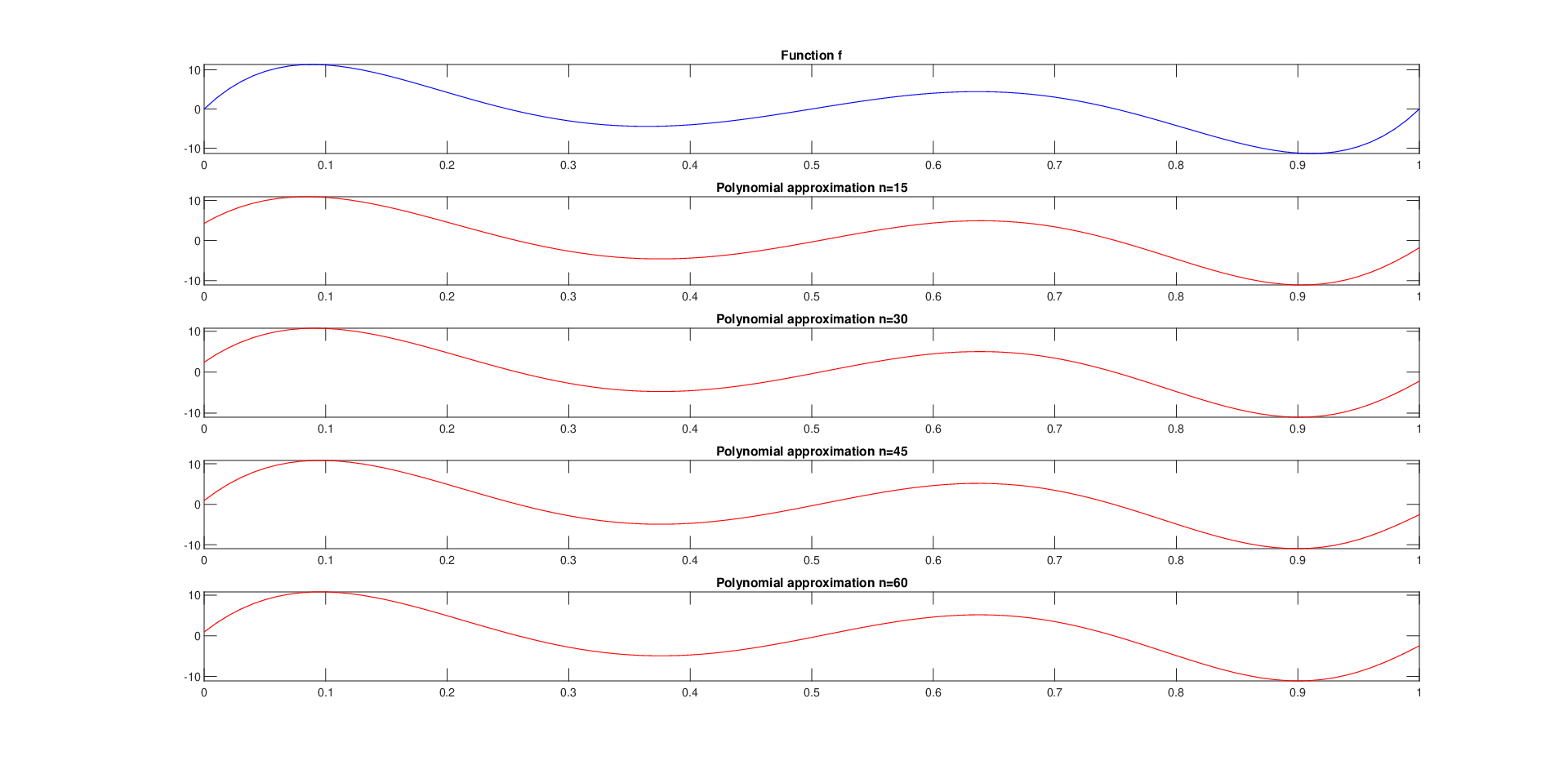
To illustrate our results let us solve numerically ( B ) for the particular function

f(t)=10^{2}t(2t-1)(t-1)(4t-1)(4t-3)

and $e_{j}$ the canonical base of polynomials, that is, $e_{j}(t):=t^{i}$ . We use an ergodic measure preserving transformation $T(t)=t+\alpha\mod 1$ , with some $\alpha\notin\mathbb{Q}$ , and systematically, we solve the sequence of optimization problems for a fixed point $\bar{t}\in[0,1]$

		$\displaystyle\min\quad g(x)$		( $\mathcal{B}_{n}(\bar{t})$ )
	$\displaystyle\text{ s.t. }$	$\displaystyle x\in M(T^{k}(\bar{t})),\;k=1,...,n.$		( $\mathcal{B}_{n}(\bar{t})$ )

In Figure 1 we show the results of the polynomial approximation found solving Problem ( ⁢ B n ( ¯ t ) ) for different values of $n$ and for point $\bar{t}=0$ and $\alpha=\sqrt{7}$ .

Refer to caption — Figure 1: Polynomial approximation with $q=10$ , $\bar{t}=\sqrt{5}$ and $\alpha=\sqrt{7}$

5.2 Rotation on the $2$ -dimensional Unit Sphere

Let us consider the following optimization problem

		$\displaystyle\min g(x,y)$
	$\displaystyle\text{s.t. }$	$\displaystyle\alpha x+\beta y\leq 6\;$	$\displaystyle\text{ for all }(\alpha,\beta)\in\mathbb{S}^{1},$

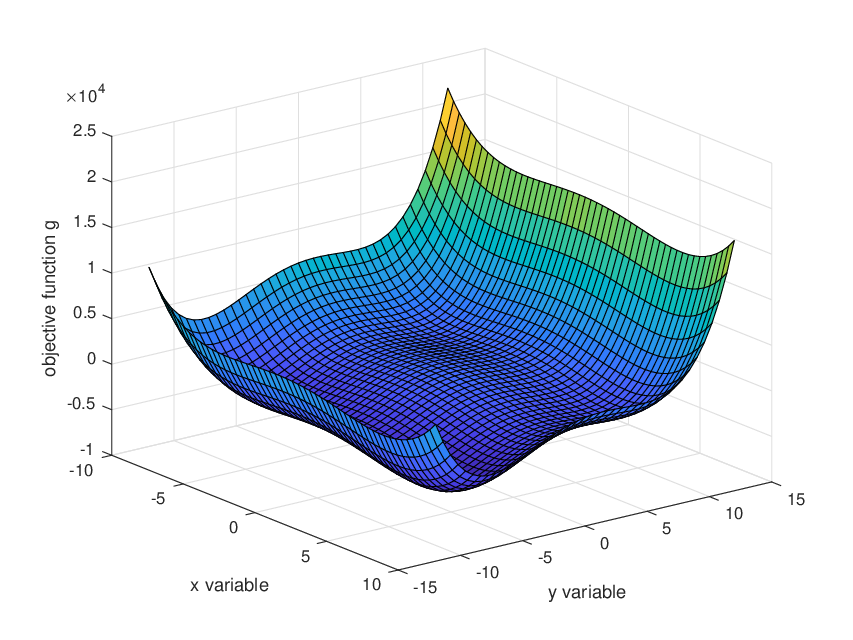
where $g$ is a non-convex polynomial function with several local-minima (see Figure 2), more precisely we choose

\displaystyle g(x,y)=(x+5)(x+2)(x-1)(x-9)+y(y+11)(y-4)(y-5)+xy.

and $\mathbb{S}^{1}$ is the $2$ -dimensional unit sphere, that is to say, $\mathbb{S}^{1}:=\{(\alpha,\beta)\in\mathbb{R}^{2}:\alpha^{2}+\beta^{2}=1\}$ . It is not difficult to see that the above problem is noting more than

		$\displaystyle\min g(x,y)$		(16)
	$\displaystyle\text{s.t. }$	$\displaystyle x^{2}+y^{2}\leq 36.$		(16)

To solve this problem, we use an irrational rotation $T:\mathbb{S}^{1}\to\mathbb{S}^{1}$ , that is, $T(\xi)=\xi\cdot e^{2\pi\theta i}$ with $\theta\in[0,1]\backslash\mathbb{Q}$ . Here the multiplication is in the sense of complex numbers. Therefore, we have to numerically solve the following optimization problems

		$\displaystyle\min g(x,y)$		( $\mathcal{U}_{n}(\xi)$ )
	$\displaystyle\text{s.t. }$	$\displaystyle x\in U_{n}(\xi)$		( $\mathcal{U}_{n}(\xi)$ )

where $U_{n}(\xi):=\{(x,y)\in\mathbb{R}^{2}:\langle T^{k}(\xi),(x,y)\rangle\leq 6,\;\forall k=1,\ldots,n\}$ .

First, we have that the global minimum of $g$ is attained at $(x_{u},y_{u})=(6.3442,-7.6398)$ and the minimum is $g(x_{u},y_{u})=-5490.9$ . On the other hand the optimal value of (16) is attained at $(x_{c},y_{c})=(3.2004,-5.0752)$ with value $g(x_{c},y_{c})=-3519.1$ . In Table 1 we can compare different numerical solutions to Problem ( ⁢ U n ( ξ ) ).

$\xi$	$n$	$v(g,U_{n}(\xi))$	$x$	$y$	$n$	$v(g,U_{n}(\xi))$	$x$	$y$
$e^{i{\pi}/{10}}$	5	-3862.4	1.7623	-6.7866	15	-3634.7	3.3542	-5.1543
$e^{i{\pi}/{6}}$	5	-4257.4	2.6753	-6.9991	15	-3519.3	3.0438	-5.1746
$e^{i{\pi}/{3}}$	5	-5406.3	5.7143	-7.2882	15	-3651.6	4.3877	-4.5573
$e^{i{4\pi}/{3}}$	5	-4258.3	4.3254	-5.5167	15	-3633.0	3.1903	-5.2573
$e^{i{7\pi}/{4}}$	5	-5251.2	4.9946	-7.5369	15	-3745.8	3.9081	-4.9747
$e^{i{\pi}/{10}}$	30	-3519.4	3.3562	-4.9778	40	-3519.4	3.3562	-4.9778
$e^{i{\pi}/{6}}$	30	-3519.3	3.0438	-5.1746	40	-3519.3	3.1230	-5.1243
$e^{i{\pi}/{3}}$	30	-3542.3	3.1288	-5.1560	40	-3542.3	3.0304	-5.2028
$e^{i{4\pi}/{3}}$	30	-3534.0	3.6424	-4.8220	40	-3534.0	3.5479	-4.8771
$e^{i{7\pi}/{4}}$	30	-3524.0	3.6397	-4.8089	40	-3524.0	3.6397	-4.8089
$e^{i{\pi}/{10}}$	70	-3519.4	3.3562	-4.9778	100	-3.5194	3.3562	-4.9778
$e^{i{\pi}/{6}}$	70	-3519.3	3.1232	-5.1242	100	-3.5193	3.1232	-5.1242
$e^{i{\pi}/{3}}$	70	-3532.1	3.0304	-5.2028	100	-3.5219	2.9323	-5.2494
$e^{i{4\pi}/{3}}$	70	-3529.4	3.4538	-4.9319	100	-3.5268	3.3599	-4.9866
$e^{i{7\pi}/{4}}$	70	-3523.6	3.5467	-4.8655	100	-3.5228	3.4538	-4.9220

Table 1: Numerical solution of Problem ( ⁢ U n ( ξ ) ).

6 Conclusion and Perspectives

In this paper, we have studied the consistency of a new method for solving robust optimization problems. In counterpart to classical methods in stochastic programming, it is based on ergodic measure preserving transformation instead of sample approximation.

In particular, our approach is more general, because we can recover the results based on samples using the shift on the denumerable product of the probability space. Moreover, our results allow us to apply the technique to infinite programming problems under reasonable assumptions, and without any compactness assumption on the index set, as classical results in this field.

We believe that our analysis represents a first step in the understanding of a new approach based on ergodicity instead of a sequence of samples. A natural question relies on to understand the relation between the choice of the measure preserving transformation and the rate of convergence of the approximate sequence of minimizers.

It is important to mention that in our result a regularization of the objective function is considered in each step, that is the role of the sequence $g_{n}$ in Theorem 3.1 and its corollaries. In most important applications, constraints are given by systems of possible nonsmooth inequalities. Commonly, this nonsmoothness is handled by using smooth regularizations, for instance, Moreau envelopes and regularization via mollifiers (see, e.g., Rockafellar_wets_book1998). Therefore, it will be necessary the study of the consistency of a method which in each step use both a regularization of the constraints and our ergodic approach.

Therefore, we plan to investigate these possible extensions of our presented method in a future paper.

Acknowledgements First, the author would like to acknowledge the helpful discussions and great comments about this work given by Professor Marco A. López Cérda, which improved notably the quality of the presented manuscript. Second, the author is grateful to the anonymous reviewers for their valuable suggestions and comments about the work, which increases the presentation of the current version of the manuscript.

References

[1] Z. Artstein and R. J.-B. Wets. Consistency of minimizers and the SLLN for stochastic programs. J. Convex Anal., 2(1-2):1–17, 1995.
[2] H. Attouch. Variational convergence for functions and operators. Applicable Mathematics Series. Pitman (Advanced Publishing Program), Boston, MA, 1984.
[3] J.-P. Aubin and H. Frankowska. Set-valued analysis. Modern Birkhäuser Classics. Birkhäuser Boston, Inc., Boston, MA, 2009. Reprint of the 1990 edition [MR1048347].
[4] A. Ben-Tal, L. El Ghaoui, and A. Nemirovski. Robust optimization. Princeton Series in Applied Mathematics. Princeton University Press, Princeton, NJ, 2009.
[5] D. Bertsimas, D. B. Brown, and C. Caramanis. Theory and applications of robust optimization. SIAM Rev., 53(3):464–501, 2011.
[6] G. C. Calafiore and M. C. Campi. The scenario approach to robust control design. IEEE Trans. Automat. Control, 51(5):742–753, 2006.
[7] M. C. Campi and S. Garatti. Wait-and-judge scenario optimization. Mathematical Programming, 167(1):155–189, 2018.
[8] M. C. Campi, S. Garatti, and M. Prandini. The scenario approach for systems and control design. Annual Reviews in Control, 33(2):149–157, 2009.
[9] M. C. Campi, S. Garatti, and F. A. Ramponi. Non-convex scenario optimization with application to system identification. In 2015 54th IEEE Conference on Decision and Control (CDC), pages 4023–4028, Dec 2015.
[10] A. Carè, S. Garatti, and M. C. Campi. Scenario min-max optimization and the risk of empirical costs. SIAM J. Optim., 25(4):2061–2080, 2015.
[11] C. Castaing and M. Valadier. Convex analysis and measurable multifunctions. Lecture Notes in Mathematics, Vol. 580. Springer-Verlag, Berlin-New York, 1977.
[12] Y. Coudène. Ergodic theory and dynamical systems. Universitext. Springer-Verlag London, Ltd., London; EDP Sciences, [Les Ulis], 2016. Translated from the 2013 French original [ MR3184308] by Reinie Erné.
[13] M. A. Goberna and M. A. López. Linear semi-infinite optimization, volume 2 of Wiley Series in Mathematical Methods in Practice. John Wiley & Sons, Ltd., Chichester, 1998.
[14] R. Hettich and K. O. Kortanek. Semi-infinite programming: theory, methods, and applications. SIAM Rev., 35(3):380–429, 1993.
[15] S. Hu and N. S. Papageorgiou. Handbook of multivalued analysis. Vol. I, volume 419 of Mathematics and its Applications. Kluwer Academic Publishers, Dordrecht, 1997. Theory.
[16] L. A. Korf and R. J.-B. Wets. Random-lsc functions: an ergodic theorem. Math. Oper. Res., 26(2):421–445, 2001.
[17] M. A. López and G. Still. Semi-infinite programming. European J. Oper. Res., 180(2):491–518, 2007.
[18] A. Prékopa. Stochastic programming, volume 324 of Mathematics and its Applications. Kluwer Academic Publishers Group, Dordrecht, 1995.
[19] F. A. Ramponi. Consistency of the scenario approach. SIAM J. Optim., 28(1):135–162, 2018.
[20] R. T. Rockafellar and R. J.-B. Wets. Variational analysis, volume 317 of Grundlehren der Mathematischen Wissenschaften [Fundamental Principles of Mathematical Sciences]. Springer-Verlag, Berlin, 1998.
[21] A. Shapiro, D. Dentcheva, and A. Ruszczyński. Lectures on stochastic programming, volume 9 of MOS-SIAM Series on Optimization. Society for Industrial and Applied Mathematics (SIAM), Philadelphia, PA; Mathematical Optimization Society, Philadelphia, PA, second edition, 2014. Modeling and theory.
[22] M. Tahanan, W. van Ackooij, A. Frangioni, and F. Lacalandra. Large-scale unit commitment under uncertainty. 4OR, 13(2):115–171, 2015.
[23] W. van Ackooij, I. Danti Lopez, A. Frangioni, F. Lacalandra, and M. Tahanan. Large-scale unit commitment under uncertainty: an updated literature survey. Ann. Oper. Res., 271(1):11–85, 2018.
[24] P. Walters. An introduction to ergodic theory, volume 79 of Graduate Texts in Mathematics. Springer-Verlag, New York-Berlin, 1982.

Ergodic Approach to Robust Optimization and Infinite Programming Problems

Abstract

Keywords:

MSC

1 Introduction

2 Notation and Preliminary

Definition 1

Definition 2

Lemma 1

Proposition 1

3 Consistency of the Approach to Robust Optimization Problems

Theorem 3.1

Proof

Corollary 1

Proof

4 Applications

4.1 Consistency of Nonconvex Scenario Approach

Theorem 4.1

Proof

Remark 1

Corollary 2

Remark 2

Corollary 3

Proof

4.2 Application to Infinite Programming Problems

Corollary 4

Proof

Corollary 5

Proof

5 Numerical Examples

5.1 Best Functional Approximation

5.2 Rotation on the 22-dimensional Unit Sphere

6 Conclusion and Perspectives

References

5.2 Rotation on the $2$ -dimensional Unit Sphere