Numerical Simulations of an Initially Top-Hat Jet and the Afterglow of GW170817 / GRB170817A

The first gravitational wave (GW) detection of a binary neutron star (NS) merger, GW 170817 (Abbott et al. 2017a), was accompanied by the first electromagnetic counterpart to any GW detection – the weak, short duration gamma-ray burst, GRB 170817A (Abbott et al. 2017b), that originated in the nearby ($D\approx 40\,$Mpc) elliptical galaxy NGC 4993 (Coulter et al. 2017). An impressive observational campaign detected the quasi-thermal kilonova emission in the NIR-optical-UV energy bands over the next few weeks (see, e.g., Abbott et al. 2017c, and references therein). The non-thermal afterglow emission was detected after $8.9\,$days in X-rays (Troja et al. 2017) and after $16.4\,$days in the radio (Hallinan et al. 2017).

GW 170817/GRB 170817A’s long-lived X-ray to radio afterglow emission was highly unusual. In contrast to the flux decay seen in almost all GRB afterglows, it showed an exceptionally long-lasting flux rise, as $F_{\nu}(t_{\rm{obs}})\propto\nu^{-0.6}t_{\rm{obs}}^{0.8}$, up to the peak at $t_{\rm{obs,pk}}\sim 150\,$days post merger (Margutti et al. 2018; Mooley et al. 2018a, e.g.), followed by a sharp decay as $F_{\nu}\propto{}t_{\rm{obs}}^{a}$ where $a\simeq-2.2$ (Mooley et al. 2018b; van Eerten et al. 2018). The broadband (X-rays, radio, and late-time optical) afterglow emission is consistent with arising from a single power-law segment (PLS) of the afterglow synchrotron spectrum, $\nu_{m}\leq\nu\leq\nu_{c}$.¹¹ 1 Here $\nu_{m}$ is the synchrotron frequency of minimal energy electrons and $\nu_{c}$ of electrons that cool on the dynamical time (Sari et al. 1998).

Almost all successful off-axis jet models for this afterglow have an angular profile that is either a (quasi-) Gaussian or a narrow core with sharp power-law wings (Lamb & Kobayashi 2018; Lazzati et al. 2018; Troja et al. 2017; D’Avanzo et al. 2018; Gill & Granot 2018; Margutti et al. 2018; Resmi et al. 2018; Troja et al. 2018). Moreover, several works have argued that a top-hat jet can be ruled out (Margutti et al. 2018; Mooley et al. 2018a, e.g.,) since it would produce a very sharp initial flux rise ($F_{\nu}\propto{}t_{\rm{obs}}^{a}$ with $a\gtrsim 3$) compared to the observed one. Such a sharp initial flux rise was obtained both numerically from 2D hydrodynamic simulations (van Eerten & MacFadyen 2011; Granot et al. 2018a, e.g.,), and analytically assuming an idealized top-hat jet (Granot et al. 2002; Eichler & Granot 2006; Nakar & Piran 2018, e.g.,)

Here we show that while an idealized top-hat jet would indeed produce sharply rising early lightcurves for off-axis observers, a more realistic description of the dynamics (using numerical simulations) for an initially top-hat jet leads to a much shallower flux rise that can explain the GRB 170817A afterglow observations (lightcurves, flux centroid motion, and upper limits on the image size). The main difference arises since within the simulation’s first dynamical time an initial top-hat jet develops a bow-shock like angular structure, which produces afterglow emission resembling that from a core-dominated structured jet,²² 2 I.e. a jet in which most of the energy resides within a narrow core, outside of which the energy per solid angle sharply drops. with a much shallower flux rise, making the two models practically indistinguishable at $t_{\rm{}obs}\gtrsim{}t_{\rm{obs,pk}}$, and not always that easy to distinguish between even at earlier times. Numerical simulations have a finite lab-frame start time, $t=t_{0}>0$, thus missing contributions to $F_{\nu}$ from $t<t_{0}$. This is often compensated for by adding emission at $t<t_{0}$ from a conical wedge from the Blandford & McKee 1976 spherical self-similar solution (van Eerten et al. 2012; De Colle et al. 2012a; De Colle et al. 2012b; Bietenholz et al. 2014; Granot et al. 2018b; Granot et al. 2018a, e.g.,). This still results in an unphysically sharp flux rise at early observed times, $t_{\rm{obs}}\lesssim 2t_{\rm{obs},0}$, corresponding to lab-frame times $t\lesssim 2t_{0}$.

The effects of $t_{0}$ including $t_{\rm{obs},0}(\theta_{\rm{obs}},t_{0})$ are analytically explained in § II. The effect of starting the simulations with a larger Lorentz factor (LF) $\Gamma_{0}=\Gamma(t_{0})$ and correspondingly smaller $t_{0}$ is shown in § III through 2D relativistic hydrodynamic simulations. In § IV model scalings and the minimal energy and circum-burst medium density estimates are provided. In § V we calculate and compare the flux centroid location and the image size and shape with radio afterglow measurements of GW 170817/GRB 170817A. Our conclusions are discussed in § VI.

We perform 2D relativistic hydrodynamical simulations with initial conditions of a conical wedge of half-opening angle $\theta_{0}$ taken out of the BM76 solution. This initially narrow and relativistic jet expands into a cold circum-burst medium (CBM) with a power-law rest-mass density profile with radius $R$ from the central source, $\rho(R)=AR^{-k}$, where for uniform (wind-like) density environment $k=0$ $(k=2)$. The BM76 spherical self-similar phase occurs after the original outflow is significantly decelerated and most of the energy is in the shocked CBM behind the forward (afterglow) shock. The material just behind the shock moves with velocity $\beta c$, with $c$ being the speed of light, and bulk LF $\Gamma=(1-\beta^{2})^{-1/2}=\Gamma_{\rm{shock}}/\sqrt{2}$. The BM76 phase reasonably holds for a top-hat jet while $\Gamma>1/\theta_{0}$ (assuming $\Gamma_{0}\theta_{0}\gg 1$, as typically inferred for GRBs) before significant lateral spreading can occur.

The radial width behind the forward shock containing most of the blastwave’s energy is $\Delta\sim 0.1\,R/\Gamma^{2}$. During the BM76 self-similar phase $\Gamma^{2}R^{3-k}=\Gamma_{0}^{2}R_{0}^{3-k}=(17-4k)E_{\rm{k,iso}}/16\pi{}Ac^{2}={\rm{const}}$, with $R_{0}=R(t_{0})\approx{}ct_{0}$ being the initial shock radius. Thus the initial radial width $\Delta_{0}=\Delta(t_{0})\sim 0.1R_{0}/\Gamma_{0}^{2}\propto{}R_{0}^{4-k}\propto\Gamma_{0}^{-2(4-k)/(3-k)}$ ($\propto\Gamma_{0}^{-8/3}$ for $k=0$) becomes much narrower and harder to resolve for larger $\Gamma_{0}$ or correspondingly smaller $t_{0}\approx{}R_{0}/c\propto\Gamma_{0}^{-2/(3-k)}$ ($\propto\Gamma_{0}^{-2/3}$ for $k=0$). This practically limits $\Gamma_{0}$ from above and $t_{0}$ from below.

An on-axis observer ($\theta_{\rm{}obs}<\theta_{0}$) receives the first photons from the simulation after a radial time delay of

$z$ being the source’s cosmological redshift. For an off-axis observer ($\Delta\theta\equiv\theta_{\rm{}obs}-\theta_{0}>0$), there is an additional angular time delay,

(Granot et al. 2017, e.g.,), which dominates the total time delay $t_{\rm{obs},0}=t_{\rm{obs},r}+t_{\rm{obs},\theta}\approx{}t_{\rm{obs},\theta}$ for $\Delta\theta>1/\Gamma_{0}$. For such off-axis viewing angles one can conveniently express $\Gamma_{0}\propto{}t_{\rm{obs},0}^{-(3-k)/2}$, which for $k=0$, $E_{\rm{k,iso}}\approx(2/\theta_{0}^{2})E$ and $z\ll 1$ gives

where for the numerical value we normalize by our best-fit model parameters derived in § III, for which $t_{\rm{obs},0}=38.1,\,23.0,\,18.3\;$days for $\Gamma_{0}=20,\,40,\,60$.

The compactness argument implies that GRB jets typically have $\Gamma_{0}\gtrsim 100$ for the emission region to be optically thin to $\gamma\gamma$-annihilation (Lithwick & Sari 2001, e.g.). Such large $\Gamma_{0}$ are very difficult to simulate, and current numerical works usually set $\Gamma_{0}\sim 20-25$ (van Eerten & MacFadyen 2013, see, however,).

Simulations initialized at $t_{0}$ do not contribute any flux at $t_{\rm{obs}}<t_{\rm{obs},0}$ (see Fig. 1). Over the first dynamical time ($t_{0}<t\lesssim 2t_{0}$), as the simulated jet relaxes from its artificially sharp top-hat initial condition, the flux sharply rises at times $t_{\rm{obs},0}\leq{}t_{\rm{obs}}\lesssim 2t_{\rm{obs},0}$, after which the flux evolves smoothly with time. During this relaxation phase, the top-hat jet is slowed down due to its interaction with the CBM and develops a bow-shock like structure (Granot et al. 2001; van Eerten & MacFadyen 2011; De Colle et al. 2012b, e.g.). Its structure at this point resembles a ‘structured jet’ with a highly energetic core, whose velocity is almost radial, surrounded by less energetic slower-moving material whose velocity points more sideways. Therefore, an initially top-hat jet inevitably transforms into a structured jet. The slower material at angles $\theta>\theta_{0}$ has a much wider beaming cone and its emission starts dominating the off-axis flux. As the jet gradually decelerates, its beaming cone widens and off-axis observers start to receive flux from smaller $\theta$ closer to the jet’s core, resulting in a more gradual flux rise compared to an analytic perpetually sharp-edged jet.

To compensate for the missing flux at $t_{\rm{obs}}<t_{\rm{obs},0}$, as shown in Fig. 1, lightcurves derived from numerical simulations are often supplemented with synthetic lightcurves obtained for the initial conditions (van Eerten et al. 2012; De Colle et al. 2012a; De Colle et al. 2012b; Bietenholz et al. 2014; Granot et al. 2018b; Granot et al. 2018a, usually a conical wedge from the BM76 self-similar solution, e.g.,) over a wide range of earlier lab-frame times, $t_{*}<t<t_{0}$ with $t_{*}\ll{}t_{0}$. We also compare the lightcurve obtained from the publicly available afterglow modeling code BOXFITv2 (van Eerten et al. 2012), which has been widely used to fit afterglow observations of GRB 170817A. Lightcurves obtained from our numerical simulations are in excellent agreement with that obtained from BOXFITv2.

The observed flux density is given by (Granot 2005; Granot & Ramirez-Ruiz 2012, e.g.)

where $d_{L}(z)$ is the luminosity distance, the $\delta$-function, $\delta_{t}=\delta\left(t-t_{\rm{obs}}/(1+z)-R\tilde{\mu}/c\right)$, accounts for the photon arrival times (Granot et al. 1999), $R\tilde{\mu}=\hat{n}\cdot\vec{R}$ where $\hat{n}$ is the direction to the observer and $\vec{R}$ is the radius vector (measured from the central source) of each fluid element having velocity $\vec{v}=\vec{\beta}c$ and Doppler factor $\delta_{D}=[\Gamma(1-\hat{n}\cdot\vec{\beta})]^{-1}$. For radial velocities (e.g. a spherical shell), $\hat{n}\cdot\vec{\beta}=\beta\tilde{\mu}$ and $\delta_{D}\approx 2\Gamma/[1+(\Gamma\tilde{\theta})^{2}]$ for $\Gamma\gg 1$. In Eq. (4), $F_{\nu}\propto\delta_{D}^{3}L^{\prime}_{\nu^{\prime}}$ holds where $L^{\prime}_{\nu^{\prime}}$ and $\delta_{D}$ are those of the part of the source that dominates the observed emission, which for a top-hat jet viewed off-axis is within an angle $\sim\max(\Gamma^{-1},\Delta\theta)$ of the point in the jet closest to the observer (where $\tilde{\theta}\approx\Delta\theta$), occupying a solid angle $\Omega_{*}\sim\min[\max(\Gamma^{-2},\Delta\theta^{2}),\theta_{0}^{2}]$. During the early flux-rising phase while the radiation is beamed away from the observer ($\Gamma>1/\Delta\theta$), $\Omega_{*}={\rm{const}}$ and one can use the scalings of $L^{\prime}_{\nu^{\prime}}$ for a spherical flow, $L^{\prime}_{\nu^{\prime}}\propto{}R^{a}\nu^{\prime b}\propto{}R^{a}\delta_{D}^{-b}$, where the PLS-dependent power-law indices $a$ and $b$ are explicitly calculated in Granot 2005. Therefore, $F_{\nu}\propto\delta_{D}^{3-b}R^{a}$ where (Salmonson 2003; Granot 2005, e.g.) $\delta_{D}\approx 2/\Gamma\Delta\theta^{2}\propto{}R^{(3-k)/2}\Longrightarrow{}F_{\nu}\propto{}R^{[2a+(3-k)(3-b)]/2}$. For GRB 170817A, PLS G is relevant and $a=[15-9p-2k(3-p)]/4$, $b=(1-p)/2$. From Eq. (2), $t_{\rm{obs}}\propto{}R$ which implies $F_{\nu}\propto{}t_{\rm{obs}}^{3(5-p)/2}$ for a uniform CBM ($k=0$).

In Fig. 1, we show the extension of the lightcurve to $t_{\rm{obs}}<t_{\rm{obs},0}$, where we reproduce the analytic flux scaling derived above. It is clear that BOXFITv2 also supplements the lightcurve at early times ($t<t_{0}\Leftrightarrow{}t_{\rm{obs}}<t_{\rm{obs},0}$) with the flux from a conical wedge out of the BM76 self-similar solution (also used for the initial conditions). Although BOXFITv2 allows the user to not include this extension in the final lightcurve, many works indeed do include it, even when fitting to observations. Either way, the flux at $t_{\rm{obs}}\lesssim 2t_{\rm{obs},0}$ is strongly affected by the rather arbitrary simulation start time $t_{0}$. Initializing the simulation at a smaller $t_{0}$ corresponding to a larger $\Gamma_{0}$ would shift this feature to earlier times and recover the much shallower flux rise in the lightcurve.

Here we show results of 2D hydrodynamic simulations using the special-relativistic hydrodynamics code Mezcal, post-processed by a complimentary radiation code (see De Colle et al. 2012a; De Colle et al. 2012b, for details). The simulations are initialized with a conical wedge of half-opening angle $\theta_{0}=0.1,\,0.2\;$rad and initial LF $\Gamma_{0}=20,\,40,\,60$ expanding into a uniform CBM ($k=0$) of rest-mass density $\rho_{0}=nm_{p}$ and number density $n$, $m_{p}$ being the proton mass. The outflow has an isotropic-equivalent kinetic energy $E_{\rm{k,iso}}=10^{53}\;$erg, corresponding to a true jet energy of $E=(1-\cos\theta_{0})E_{\rm{k,iso}}\approx 5\times 10^{50}\;$erg for $\theta_{0}=0.1$ and $E\approx 2\times 10^{51}\;$erg for $\theta_{0}=0.2$.

We consider synchrotron radiation from relativistic electrons that are accelerated at the afterglow shock to a power-law energy distribution, $dN_{e}/d\gamma_{e}\propto\gamma_{e}^{-p}$ for $\gamma_{e}>\gamma_{m}$ with $p=2.16$, which are a fraction $\xi_{e}$ of all post-shock electrons, and hold a fraction $\epsilon_{e}=0.1$ of the post-shock internal energy density, where a fraction $\epsilon_{B}=0.1$ goes to the magnetic field. The radiation is calculated numerically for a fixed set of model parameters ($E,\,n,\,\epsilon_{e},\,\epsilon_{B},\,p,\,\theta_{0}$) and for a grid of $\theta_{\rm{obs}}$ values. When including the parameter $\xi_{e}$, the set of model parameters become degenerate, where the afterglow flux is invariant under the change $E\to E/\xi_{e}$, $n\to{}n/\xi_{e}$, $\epsilon_{e}\to\epsilon_{e}\xi_{e}$, and $\epsilon_{B}\to\epsilon_{B}\xi_{e}$, for $m_{e}/m_{p}<\xi_{e}\leq 1$. We then use the scaling relations described in Granot 2012 for arbitrary values of ($E,\,n$), as well as the scaling with the shock microphysical parameters in each PLS (Granot & Sari 2002, Table 2 of). See Granot et al. 2017 for further details.

There are in total 8 model parameters, i.e. $E,\,n,\,\epsilon_{e},$ $\epsilon_{B},\,p,\,\xi_{e},\,\theta_{0},\,\theta_{\rm obs}$. There are 5 effective observational constraints: (i) the spectral index $b\approx-0.58$ ($F_{\nu}\propto\nu^{b}$; $b=[1-p]/2$ for PLS G, which determines $p=1-2b\approx 2.16$), (ii) the lightcurve peak time $t_{\rm obs,pk}\approx 150\,$days, (iii) the peak flux $F_{\nu,\rm pk}$, (iv) the shape of the lightcurve near the peak (which approximately determines $\theta_{\rm{}obs}/\theta_{0}$), (v) the radio flux centroid’s apparent velocity. These 5 constraints involve equalities and reduce the dimensionality of the allowed parameter space from an 8D to a 3D. There are also 3 additional constraints that involve inequalities and hence only reduce its volume but not its dimensionality: the fact that all the broadband afterglow observations lie within PLS G, $\nu_{m}<\nu<\nu_{c}$, and $\theta_{\rm obs}\lesssim 0.5$ from the GW detection.

Our afterglow lightcurve fitting is guided by the measured peak at $t_{\rm{obs,pk}}\sim 150\;$days (Dobie et al. 2018) and the data points near the peak. Fig. 2 shows the fit to the afterglow data for different initial $\Gamma_{0}$ (top-left panel) and viewing angles $\theta_{\rm{obs}}$ (top-right panel). We do not attempt to fit the early time data at $t_{\rm{obs}}\lesssim 40$ days, before the simulated lightcurves contain the dominant and dynamically relaxed contribution from the hydrodynamic simulation. Nevertheless, we obtain a reasonable fit to the afterglow data for different values of $\Gamma_{0}$, where our lightcurves for larger $\Gamma_{0}$ extend to earlier times and can adequately explain the data at $t_{\rm{obs}}\gtrsim 40\,$days.

The best constrained parameters are (Granot et al. 2018b, also see): (i) $p\approx 2.16$, and (ii) $\theta_{\rm{obs}}/\theta_{0}\approx 3.1\pm 0.1$, since it significantly affects the shape of the lightcurve before and around the peak time. In the bottom-right panel of Figure 2, we compare the model lightcurves for $\theta_{0}=0.1,\,0.2$ and show that in both cases $\theta_{\rm{obs}}/\theta_{0}=3.1$ provides a comparably good fit, while fixing the same values for the shock microphysical parameters but varying the true jet energy $E$ and CBM density $n$.

We compare the simulation lightcurves with those obtained from semi-analytic models of different jet structures, namely a top-hat (THJ), Gaussian (GJ), and a power law jet (PLJ) (see Gill & Granot 2018, for models of structured jets). For the top-hat jet we prescribe the same dynamics as that for the two structured jets, i.e. every part of the jet evolves locally as if it were part of a spherical flow, with no sideways spreading. As a result, all three semi-analytic models yield very similar lightcurves right after the peak when the compact core of the jet becomes visible to the off-axis observer. On the other hand, the simplified dynamics of the semi-analytic models leads to a significantly shallower post-peak flux decay rate compared to the simulated one, which may be attributed to the combination of a shallower asymptotic decay and a smaller overshoot just after the peak (Granot 2007, e.g.). The post-peak flux decay behavior of different structured jets will be investigated in more detail using 2D numerical simulations in another work (Urrutia et al. 2019, in preparation). For the semi-analytic models one set of model parameter values that can explain the observations sufficiently well are: $E_{\rm k,iso,\{c,jet\}}\approx 10^{51.6}\,$erg, $\theta_{\rm\{c,jet\}}\approx 5^{\circ}$, $\theta_{\rm obs}=27^{\circ}$, $\epsilon_{e}\approx 10^{-1}$, $\epsilon_{B}\approx 10^{-2.8}$, and the only difference is in the core Lorentz factors between the three models, with $\Gamma_{\rm c}^{\rm PLJ}=100$, $\Gamma_{\rm jet}^{\rm THJ}=\Gamma_{\rm c}^{\rm GJ}=600$.

For the lightcurve fits we assume $\xi_{e}=1$, and use the dependence on the shock microphysical parameters in PLS G from Granot & Sari 2002, now including the degeneracy due to $\xi_{e}$ (van Eerten & MacFadyen 2012, e.g.), $F_{\nu,G}\propto\epsilon_{e}^{p-1}\epsilon_{B}^{(p+1)/4}\xi_{e}^{2-p}\nu^{(1-p)/2}$. We also use the global scaling relations (Granot 2012), which are conveniently parameterized through length and time,

and through mass and energy, $\zeta=m^{\prime}/m=E^{\prime}/E$, where the rescaled parameters are denoted with a prime, $\mathcal{F}=F^{\prime}_{\nu,G}(t^{\prime}_{\rm{obs}},\epsilon^{\prime}_{e},\epsilon^{\prime}_{B},\xi^{\prime}_{e})/F_{\nu,G}(t_{\rm{obs}},\epsilon_{e},\epsilon_{B},\xi_{e})$,

Next, we constrain $E$ from below by using these scaling relations and our (partly degenerate) best-fit parameters: $E=10^{50.4}\;{\rm{erg}}$, $n=10^{-3.6}\;{\rm{}cm^{-3}}$, $\epsilon_{e}=10^{-1.8}$, $\epsilon_{B}=10^{-3.12}$, $\theta_{\rm{obs}}/\theta_{0}=3.1$ (fixing $\xi_{e}=1$, $p=2.16$, $\theta_{0}=0.1$). Matching the peak time of the simulated lightcurve to $t_{\rm{obs,pk}}\approx 150\,$days requires no significant time rescaling, and yields $\alpha=t^{\prime}_{\rm{obs}}/t_{\rm{obs}}\approx 1$. Matching the peak flux to that observed requires equating Eq. (6) to unity. Altogether, replacing the unprimed quantities by the best-fit values, and then making the rescaled quantities unprimed, and solving for $\zeta$, yields

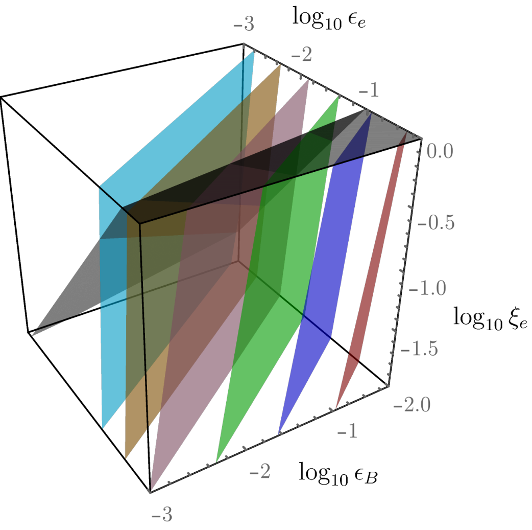
where the equality in Eq. (7) results from Eq. (5) when $\alpha=1$. This leaves us with a 3D allowed parameter space since we started with 7 free model parameters ($\theta_{0}=0.1$ was fixed by the simulation, leaving $E,\,n,\,\epsilon_{e},$ $\epsilon_{B},\,p,\,\xi_{e},\,\theta_{\rm obs}$) and used 4 observational constraints. The jet energy in Eq. (7) decreases with increasing $\epsilon_{e},\,\epsilon_{B}$ and increases only weakly with $\xi_{e}$. A minimal energy constraint can be obtained by maximizing the values of $\epsilon_{e},\,\epsilon_{B}$ and minimizing that of $\xi_{e}$. This is demonstrated in Fig. 3, where we show planes in the 3D parameter space [$\xi_{e},\epsilon_{e},\epsilon_{B}$] for different jet energies. Here we first use the fact that the broadband afterglow observations lie on a single PLS, with $\nu>\nu_{m}$, where we obtain

for $t_{\rm obs,150d}=t_{\rm obs}/(150\,{\rm days})$ and $p=2.16$ from the expression for PLS G given in Granot & Sari 2002. This expression is only valid for a spherical flow and for an on-axis observer, for whom the flux is dominated by emission from material along the LOS. At $t_{\rm obs}\geq t_{\rm obs,pk}\approx 150\,$days, the flux is dominated by that from the core of the jet with $E_{\rm k,iso,c}\lesssim 10^{52.7}\,$erg. At $t_{\rm obs}<t_{\rm obs,pk}$, the flux is dominated by emission from material outside of the core at $\theta>\theta_{0}$ with $E_{\rm k,iso}<E_{\rm k,iso,c}$. To obtain the value of $\nu_{m}$ for an off-axis observer, we calibrated Eq. (8) by comparing it with the value of $\nu_{m}$ obtained from our numerical simulation around the time of the earliest radio observations at $t_{\rm obs}\approx 16.4\,$days. Next, we use the relation from Eq. (7) in Eq. (8) and replace $E_{\rm k,iso}$ to obtain an expression that depends only on shock microphysical parameters, which, for $\nu_{m}({\rm 16.4~days})<\nu_{\rm obs}=3\,$GHz, yields a lower limit on $\xi_{e}$

This constraint is shown as a shaded black plane in Fig. 3 above which Eq. (7) is satisfied. Another useful constraint here is that $\xi_{e,\min}<1$, which yields

We first use the constraint on $\xi_{e}$ from Eq. (9) in Eq. (7) and remove the dependence on $\xi_{e}$. Next, we use the additional constraint on $\epsilon_{e}$ from Eq. (10) (which is equivalent to substituting $\xi_{e}=1$ and $\epsilon_{e}=\epsilon_{e,\max}$ in Eq. [7]) to obtain

as also demonstrated in Fig. 3 by the intersection of the black plane with planes marked by jet energies $E>E_{\min}$.

If we consider only some $\xi_{e}<1$, as may be expected on theoretical grounds, then Eq. (9) will lead to $\epsilon_{e,\max}=0.12\epsilon_{B,-1}^{-1/6}\xi_{e}^{7/6}$ and accordingly increase $E_{\min}$ to

Finally, according to Eq. (7) $E_{\min}$ also corresponds to a minimal CBM density,

We compare the afterglow image size and flux centroid motion on the plane of the sky as obtained from our simulations to the GW 170817/GRB 170817A radio observations. VLBI observations between 75 and $230\,$days revealed an unresolved source whose flux centroid showed apparent superluminal motion with $\langle v_{\rm{app}}\rangle/c=\langle\beta_{\rm{app}}\rangle=4.1\pm 0.5$ (Mooley et al. 2018b). The flux centroid’s location on the plane of the sky is defined as

(Granot et al. 2018a, e.g.,), where $dF_{\nu}=I_{\nu}d\Omega=I_{\nu}{}d_{A}^{-2}dS_{\perp}$, with $I_{\nu}$ being the specific intensity, $d_{A}$ the angular distance, and $dS_{\perp}=d\tilde{x}\,d\tilde{y}$ a transverse area element on the plane of the sky. The jet symmetry axis is in the $\tilde{x}$-$\tilde{z}$ plane, where the $\tilde{z}$-axis points to the observer. Because of the flow’s axisymmetry, the image has the reflection symmetry $I_{\nu}(\tilde{x},\tilde{y})=I_{\nu}(\tilde{x},-\tilde{y})$. Therefore, $\mathbf{\tilde{r}}_{\rm fc}=(\tilde{x}_{\rm{fc}},0)$ and the flux centroid moves along the $\tilde{x}$-axis. Since $I_{\nu}=d_{A}^{2}dF_{\nu}/dS_{\perp}\propto{}F_{\nu}/S_{\perp}$ where $S_{\perp}\propto\ell^{2}$, it scales in PLS G as $\mathcal{I}=I^{\prime}_{\nu,G}(t^{\prime}_{\rm{obs}},\tilde{x}^{\prime},\tilde{y}^{\prime})/I_{\nu,G}(t_{\rm{obs}},\tilde{x},\tilde{y})$,

The image size, flux centroid location, and observed time all scale as $\alpha=\tilde{x}^{\prime}/\tilde{x}=\tilde{y}^{\prime}/\tilde{y}=\tilde{x}^{\prime}_{\rm{fc}}/\tilde{x}_{\rm{fc}}=t^{\prime}_{\rm{obs}}/t_{\rm{obs}}$, independent of the r.h.s of Eq. (15). The flux centroid’s apparent velocity $\beta_{\rm{app}}$ remains unchanged, but shifts to the rescaled observer time (see, e.g. Sec. 4 of Granot et al. 2018a, for more details).

Fig. 4 shows how our best-fit simulated $\langle\beta_{\rm{app}}\rangle$ varies with $\alpha$. The measured $\langle\beta_{\rm{app}}\rangle=4.1\pm 0.5$ corresponds to $\alpha=0.661^{+0.242}_{-0.141}$, and is consistent (at the 1.35$\sigma$ level) with our fiducial model that fits the afterglow lightcurve ($\alpha=1$), which thus passes an important consistency check.

To calculate the afterglow image size and shape, we fit the surface brightness to an elliptical Gaussian, $I_{\nu}\propto\exp[-(\tilde{x}-\tilde{x}_{\rm{el}})^{2}/2\sigma_{x}^{2}-\tilde{y}^{2}/2\sigma_{y}^{2}]$ centered at $(\tilde{x}_{\rm{el}},0)$, where $(\sigma_{x},\sigma_{y})$ are the standard deviations of the semi-minor and semi-major axes along the $\tilde{x}$-axis and $\tilde{y}$-axis, respectively (Granot et al. 2018a). The top-panel of Fig. 5 shows the evolution of the afterglow flux-centroid location, and the afterglow image size and shape for $\alpha=1$ and for the $\langle{\beta_{\rm{app}}}\rangle$ best-fit $\alpha=0.661$. Our image size is consistent with the upper limits from radio VLBI observations (Mooley et al. 2018b; Ghirlanda et al. 2019). The bottom-panel of Fig. 5 shows the flux centroid’s location, $\tilde{x}_{\rm{fc}}(t_{\rm{obs}})$, as well as its instantaneous ($\beta_{\rm{app}}=|{}d\tilde{x}_{\rm{fc}}/d(ct_{\rm{obs}})|$) and mean ($\langle{\beta_{\rm{app}}}\rangle_{0}=|\tilde{x}_{\rm{fc}}|/ct_{\rm{obs}}$) apparent velocities, for our fiducial model ($\alpha=1$), and over the $1\sigma$ confidence interval of $\alpha$ derived in Fig. 4. We find that $\beta_{\rm{app}}(t_{\rm{obs,pk}})\approx\langle{\beta_{\rm{app}}}\rangle$.

The measured $\langle{\beta_{\rm{app}}}\rangle$ favors a slightly larger $\theta_{0}$ compared to our $\theta_{0}=0.1$. The lightcurve peak occurs when $1/\Delta\theta\approx\Gamma(t_{\rm{obs,pk}})\approx\beta_{\rm{app}}(t_{\rm{obs,pk}})\approx\langle{\beta_{\rm{app}}}\rangle$, implying $\theta_{0}\approx[\langle{\beta_{\rm{app}}}\rangle(\theta_{\rm{obs}}/\theta_{0}-1)]^{-1}\approx 0.116^{+0.016}_{-0.013}$ using the measured $\langle\beta_{\rm{app}}\rangle=4.1\pm 0.5$ and our inferred $\theta_{\rm{obs}}/\theta_{0}=3.1\pm 0.1$. The latter implies $\Gamma(t_{\rm{obs,pk}})\propto\theta_{0}^{-1}$, which in turn for the measured $t_{\rm{obs,pk}}(\theta_{0})\approx 150\,{\rm{days}}$, and either pre- or post-jet break simple analytic dynamics, implies $E/n\propto\theta_{0}^{-6}$. This agrees with the best-fit values for our $\theta_{0}=0.1,\,0.2$ to within 34%, $(0.2/0.1)^{6}(10^{50.32}/10^{-2})/(10^{50.4}/10^{-3.6})\approx 1.337$. Even for $\theta_{0}=0.2$, a derivation of $E_{\rm{min}}$ following the one done above for $\theta_{0}=0.1$ gives a result very similar to Eq. (11), implying that it is quite robust. Altogether, $\langle{\beta_{\rm{app}}}\rangle$ provides an additional observational constraint that allows us to constrain an additional model parameter, $\theta_{0}$, which still leaves us with a 3D allowed parameter space.

This work demonstrates using afterglow lightcurves and image size, shape and flux centroid motion, all derived from 2D hydrodynamical numerical simulations, that an initially top-hat jet can fit the afterglow observations of GW 170817/GW 170817A for $\theta_{0}\approx 0.1$ and $\theta_{\rm{obs}}/\theta_{0}\approx 3$ at $t_{\rm obs}\gtrsim t_{\rm obs,pk}$. We show that simulations of initially top-hat jets with a modest $\Gamma_{0}\sim 20-25$ can only be used to fit the late-time observations near the lightcurve’s peak at $t_{\rm{obs,pk}}\approx 150\,$days. Fitting earlier observations at $t_{\rm{obs}}\lesssim 60\,$days requires $\Gamma_{0}\gtrsim 25$.

We analytically express the allowed parameter space (Eqs. [7]) showing the full degeneracies between the model parameters, and find a robust lower limit on the jet’s true energy, $E_{\min}\approx 5.3\times 10^{48}\,$erg (Eq. [11]), and the CBM density, $n_{\min}\approx 5.3\times 10^{-6}~{\rm cm}^{-3}$ (Eq. [13]).

Our numerical simulations are initialized using a conical wedge from the BM76 self-similar solution; a similar setup is used in the BOXFITv2 code. The simulation is initialized at a finite lab-frame time $t_{0}=t(\Gamma_{0})$ corresponding to the modest $\Gamma_{0}=\Gamma(t_{0})$. Therefore, no flux contributions are obtained from the simulated region at $t<t_{0}\Leftrightarrow t_{\rm{obs}}<t_{\rm{obs,0}}$. Artificially supplementing the lightcurve at those times with flux arising from the initial condition (a top-hat jet) over a wide time-range produces an early sharply-rising flux for an off-axis ($\theta_{\rm{obs}}>\theta_{0}$) observer. However, within a dynamical time ($t_{0}<t\lesssim 2t_{0}\Leftrightarrow{}t_{\rm{obs,0}}<t_{\rm{obs}}\lesssim 2t_{\rm{obs,0}}$), as the outflow relaxes from the initial conditions it develops a bow-shock like angular structure that resembles a structured jet having an energetic relativistic core surrounded by mildly (and sub-) relativistic low-energy material. Outside the highly-relativistic core, whose emission is strongly beamed, the slower material makes the dominant contribution to the flux for off-axis observers due to its much wider beaming cone. As the jet’s core decelerates, its beaming cone widens and the observer sees a gradual rise in flux until the entire core becomes visible, at which point the flux peaks and starts to decline thereafter, gradually joining the on-axis lightcurve.

We demonstrate here that by using increasingly larger $\Gamma_{0}=20,\,40,\,60$ the initial observed time can be shifted to correspondingly earlier times, $t_{\rm{obs},0}=38.1,\,23.0,\,18.3\;$days, thereby replacing the sharp rise in flux with a much more gradual rise. In GRB 170817A, the shallow flux rise seen from $t_{\rm{obs,0}}\simeq 10\,$days can potentially be reproduced for $\Gamma_{0}\gtrsim 10^{2.5}$, which are physically plausible but computationally challenging, although the exact shape of the early rising lightcurve in this case is still unclear. Nevertheless, the initially top-hat jet model has some limitations. For example, the early time afterglow lightcurve shows a power-law rise ($F_{\nu}\propto t_{\rm obs}^{0.8}$) to the peak, whereas the model lightcurve has some curvature. In this work we did not carry out a detailed model fit to the data to determine the goodness of fit since our simulations were limited to $\Gamma_{0}=60$ and could not fit observations at $t_{\rm obs}\lesssim 40\,$days. Numerical simulations of structured jets that show a greater degree of complexity, and therefore are more realistic, also have larger number of model parameters, which allows them to capture the subtleties of the observed afterglow data more effectively.

Numerical simulations of a relativistic jet penetrating through the dynamical ejecta/neutrino-driven wind of BNS merger (Bromberg et al. 2018; Gottlieb et al. 2018; Xie et al. 2018; Geng et al. 2019) find that the emergent jet develops a core-dominated angular structure similar to what we find. Moreover, our afterglow model fit parameters are consistent with works featuring initially structured core-dominated jets. This renders both scenarios practically indistinguishable from afterglow observations alone, particularly close to and after the peak time of the lightcurve (Gottlieb et al. 2019, also see, e.g.,) when emission from the core starts dominating the observed flux, thereby validating the use of initially top-hat jet simulations as an attractive tool for afterglow modeling of core-dominated jets.

Both the jet’s dynamics and initial angular structure outside its core, before it is decelerated by the external medium, affects the afterglow emission before the lightcurve peak time. From the afterglow observations alone, it might be difficult to disentangle their effects, however, they may be better probed by the prompt emission. For example, in the case of GRB 170817A, its highly sub-luminous and mildly soft prompt $\gamma$-ray emission rules out an initial top-hat jet (Abbott et al. 2017b; Granot et al. 2017, e.g.,), favoring instead emission from sub-energetic mildly-relativistic material near our line of sight.

References

- Abbott et al. (2017a) Abbott, B. P., Abbott, R., Abbott, T. D., et al. 2017a, Physical Review Letters, 119, 161101
- Abbott et al. (2017b) —. 2017b, ApJ, 848, L13
- Abbott et al. (2017c) —. 2017c, ApJ, 848, L12
- Bietenholz et al. (2014) Bietenholz, M. F., De Colle, F., Granot, J., Bartel, N., & Soderberg, A. M. 2014, MNRAS, 440, 821
- Blandford & McKee (1976) Blandford, R. D., & McKee, C. F. 1976, Physics of Fluids, 19, 1130
- Bromberg et al. (2018) Bromberg, O., Tchekhovskoy, A., Gottlieb, O., Nakar, E., & Piran, T. 2018, MNRAS, 475, 2971
- Coulter et al. (2017) Coulter, D. A., Foley, R. J., Kilpatrick, C. D., et al. 2017, Science, 358, 1556
- D’Avanzo et al. (2018) D’Avanzo, P., Campana, S., Salafia, O. S., et al. 2018, A&A, 613, L1
- De Colle et al. (2012a) De Colle, F., Granot, J., López-Cámara, D., & Ramirez-Ruiz, E. 2012a, ApJ, 746, 122
- De Colle et al. (2012b) De Colle, F., Ramirez-Ruiz, E., Granot, J., & Lopez-Camara, D. 2012b, ApJ, 751, 57
- Dobie et al. (2018) Dobie, D., Kaplan, D. L., Murphy, T., et al. 2018, ApJ, 858, L15
- Eichler & Granot (2006) Eichler, D., & Granot, J. 2006, ApJ, 641, L5
- Geng et al. (2019) Geng, J.-J., Zhang, B., Kölligan, A., Kuiper, R., & Huang, Y.-F. 2019, arXiv e-prints, arXiv:1904.02326
- Ghirlanda et al. (2019) Ghirlanda, G., Salafia, O. S., Paragi, Z., et al. 2019, Science, doi:10.1126/science.aau8815
- Gill & Granot (2018) Gill, R., & Granot, J. 2018, MNRAS, 478, 4128
- Gottlieb et al. (2018) Gottlieb, O., Nakar, E., & Piran, T. 2018, MNRAS, 473, 576
- Gottlieb et al. (2019) —. 2019, arXiv e-prints, arXiv:1903.08173
- Granot (2005) Granot, J. 2005, ApJ, 631, 1022
- Granot (2007) Granot, J. 2007, in Revista Mexicana de Astronomia y Astrofisica Conference Series, Vol. 27, Revista Mexicana de Astronomia y Astrofisica, vol. 27, 140–165
- Granot (2012) —. 2012, MNRAS, 421, 2610
- Granot et al. (2018a) Granot, J., De Colle, F., & Ramirez-Ruiz, E. 2018a, MNRAS, 481, 2711
- Granot et al. (2018b) Granot, J., Gill, R., Guetta, D., & De Colle, F. 2018b, MNRAS, 481, 1597
- Granot et al. (2017) Granot, J., Guetta, D., & Gill, R. 2017, ApJ, 850, L24
- Granot et al. (2001) Granot, J., Miller, M., Piran, T., Suen, W. M., & Hughes, P. A. 2001, in Gamma-ray Bursts in the Afterglow Era, ed. E. Costa, F. Frontera, & J. Hjorth, 312
- Granot et al. (2002) Granot, J., Panaitescu, A., Kumar, P., & Woosley, S. E. 2002, ApJ, 570, L61
- Granot et al. (1999) Granot, J., Piran, T., & Sari, R. 1999, ApJ, 513, 679
- Granot & Ramirez-Ruiz (2012) Granot, J., & Ramirez-Ruiz, E. 2012, Jets and gamma-ray burst unification schemes
- Granot & Sari (2002) Granot, J., & Sari, R. 2002, ApJ, 568, 820
- Haggard et al. (2018) Haggard, D., Nynka, M., & Ruan, J. J. 2018, GRB Coordinates Network, 23137, 1
- Hajela et al. (2019) Hajela, A., Margutti, R., Fong, W., et al. 2019, GRB Coordinates Network, 24000, 1
- Hallinan et al. (2017) Hallinan, G., Corsi, A., Mooley, K. P., et al. 2017, Science, 358, 1579
- Lamb & Kobayashi (2018) Lamb, G. P., & Kobayashi, S. 2018, MNRAS, 478, 733
- Lazzati et al. (2018) Lazzati, D., Perna, R., Morsony, B. J., et al. 2018, Physical Review Letters, 120, 241103
- Lithwick & Sari (2001) Lithwick, Y., & Sari, R. 2001, ApJ, 555, 540
- Margutti et al. (2018) Margutti, R., Alexander, K. D., Xie, X., et al. 2018, ApJ, 856, L18
- Mooley et al. (2018a) Mooley, K. P., Nakar, E., Hotokezaka, K., et al. 2018a, Nature, 554, 207
- Mooley et al. (2018b) Mooley, K. P., Deller, A. T., Gottlieb, O., et al. 2018b, Nature, 561, 355
- Nakar & Piran (2018) Nakar, E., & Piran, T. 2018, MNRAS, 478, 407
- Resmi et al. (2018) Resmi, L., Schulze, S., Ishwara-Chandra, C. H., et al. 2018, ApJ, 867, 57
- Salmonson (2003) Salmonson, J. D. 2003, ApJ, 592, 1002
- Sari et al. (1998) Sari, R., Piran, T., & Narayan, R. 1998, ApJ, 497, L17
- Troja et al. (2017) Troja, E., Piro, L., van Eerten, H., et al. 2017, Nature, 551, 71
- Troja et al. (2018) Troja, E., Piro, L., Ryan, G., et al. 2018, MNRAS, 478, L18
- van Eerten et al. (2018) van Eerten, E. T. H., Ryan, G., Ricci, R., et al. 2018, arXiv e-prints, arXiv:1808.06617
- van Eerten & MacFadyen (2013) van Eerten, H., & MacFadyen, A. 2013, ApJ, 767, 141
- van Eerten et al. (2012) van Eerten, H., van der Horst, A., & MacFadyen, A. 2012, ApJ, 749, 44
- van Eerten & MacFadyen (2011) van Eerten, H. J., & MacFadyen, A. I. 2011, ApJ, 733, L37
- van Eerten & MacFadyen (2012) —. 2012, ApJ, 747, L30
- Xie et al. (2018) Xie, X., Zrake, J., & MacFadyen, A. 2018, ApJ, 863, 58