A fully implicit, scalable, conservative nonlinear relativistic Fokker-Planck 0D-2P solver for runaway electrons
Abstract
Upon application of a sufficiently strong electric field, electrons break away from thermal equilibrium and approach relativistic speeds. These highly energetic ‘runaway’ electrons ( MeV) play a significant role in tokamak disruption physics, and therefore their accurate understanding is essential to develop reliable mitigation strategies. For this purpose, we have developed a fully implicit solver for the 0D-2P (i.e., including two momenta coordinates) relativistic nonlinear Fokker-Planck equation (rFP). As in earlier implicit rFP studies (NORSE, CQL3D), electron-ion interactions are modeled using the Lorentz operator, and synchrotron damping using the Abraham-Lorentz-Dirac reaction term. However, our implementation improves on these earlier studies by 1) ensuring exact conservation properties for electron collisions, 2) strictly preserving positivity, and 3) being scalable algorithmically and in parallel. Key to our proposed approach is an efficient multigrid preconditioner for the linearized rFP equation, a multigrid elliptic solver for the Braams-Karney potentials [Braams and Karney, Phys. Rev. Lett. 59, 16 (1987)], and a novel adaptive technique to determine the associated boundary values. We verify the accuracy and efficiency of the proposed scheme with numerical results ranging from small electric-field electrical conductivity measurements to the accurate reproduction of runaway tail dynamics when strong electric fields are applied.
Los Alamos National Laboratory, New Mexico, USA
1 Introduction
Relativistic Coulomb collisions are modeled using an extended version of the Landau-Fokker-Planck collision operator [1]. Similarly to its non-relativistic counterpart [2], the operator assumes small-angle collisions, is well-posed, and features strict conservation of total particle number, total momentum, and total energy [3]. However, its accurate numerical solution is difficult because of its integro-differential formulation, which introduces scalability and discretization challenges. In this study, we propose a finite-difference-based conservative, parallel, fully implicit solver for the 0D-2P relativistic Fokker-Planck (rFP) electron-electron collision operator. This work builds and improves on earlier rFP algorithms as implemented in the NORSE [4] and CQL3D [5, 6] codes.
The solver proposed in this study is primarily designed to simulate runaway electrons produced by a large loop voltage. In tokamaks, the loop voltage induced during disruptions can produce a large amount of runaway electrons, which may severely damage plasma facing materials [7, 8]. The generated runaway current is also affected by secondary mechanisms such as energy transfers from the primary runaway electron current to the thermal electrons through knock-on (large-angle) collisions. Understanding these nonlinear mechanisms may be essential to develop either avoidance or mitigation strategies for runaway electrons in tokamaks.
A solver designed to capture runaway-electron dynamics benefits from certain features. For example, capturing small-amplitude tails necessitates strict positivity preservation. Runaway-electron generation time may be large: a sizable runaway tail length may take hundreds of electron-electron thermal collision-time scales to develop. Therefore, an implicit solver that can step over stiff thermal collision-time scales is desirable. The ability to use large time steps also demands that the scheme be asymptotic preserving, which in turn requires enforcing strict conservation properties [9]. It is also essential that the solver be optimal and scales with the number of mesh points, as resolving small-scale features may require fine grids while fitting long tails may require large domains. The relativistic Fokker-Planck operator can be expressed either in integral form [1] or in differential form [10]. We employ the differential form, in which the collisional coefficients are expressed in terms of relativistic potentials. This form is more conducive to an optimal solver, where is the number of grid points, as the integral form produces an scaling when symmetry is preserved in the integral operators (which is required to achieve strict conservation properties [11, 12]). To obtain a nearly optimal scaling (, with ) with the differential formulation, we propose a multigrid-preconditioned GMRES [13] solver for the potentials along with an adaptive treatment for evaluating potential far-field boundary conditions [which greatly decreases their computational complexity from to ]. We note that it is in principle possible to improve the scaling resulting from the integral form of the collision operator by the use of optimal integral methods such as fast multipole methods [14]. However, such methods can break the numerical symmetry of the integrals, resulting in the loss of strict conservation properties. In this regard, fast integral methods would not improve on the proposed optimal algorithm for the differential formulation, and would require similar strategies to recover the strict conservation properties of the collision operator.
With regard to time-stepping, we propose a conservative, fully implicit nonlinear scheme, which as a result is asymptotic preserving (i.e., it captures the Maxwell-Jüttner distribution as a steady-state solution to our system). Earlier algorithmic approaches proposed for this system are either linearly implicit (e.g., NORSE [4]), or lack strict conservation properties (e.g., CQL3D [5, 6]). The implicit solver proposed in this study satisfies discrete conservation properties, is preconditioned for optimal algorithmic performance, and is scalable in parallel. As a result, our algorithm scales as Our conservation and preconditioning strategies follow closely those proposed in Ref. [9].
The rest of the paper is organized as follows. In 2, we discuss the full relativistic electron-electron operator, the Lorentz operator for electron-ion interactions, and the Abraham-Lorentz-Dirac reaction term for modeling losses due to synchrotron damping. Then, in 3, we discuss the algorithmic aspects with regard to the discrete conservation strategy, positivity preservation, and our near-optimal strategy for determination of the potentials. In 4, we briefly describe our fully implicit nonlinear solver using an Anderson Acceleration scheme. In 5, we discuss the numerical results that demonstrate the correctness of our implementation, and finally in 6 we list the conclusions and scope for future work.
2 Formulation
We model a homogeneous quasi-neutral plasma. We evolve the electron species with the relativistic Fokker-Planck equation for the electron distribution function, , in the presence of background species ,
| (1) |
where is time normalized with the relativistic electron collision time,
is the momentum vector normalized with , is the electron mass, is the speed of light, is the electron charge, is the electric field normalized with the critical value for runaway electron generation [8], , is the electron number density, is the electrical permittivity, is the Coulomb logarithm, refers to the electron friction coefficients associated with synchrotron radiation damping effects (defined in detail later), and is the collision operator given by,
| (2) |
where represents the collisional diffusion tensor coefficients and represents the collisional friction vector coefficients (computed based on the appropriate background species ). Though Eq. (1) in principle may be used for multiple species, here we only consider the evolution of electrons interacting with themselves, ions and external electric fields.
The distribution function is described in a two-dimensional cylindrical domain ), with the subscripts and referring to directions parallel and perpendicular to the magnetic field, respectively (see Fig. 1). The azimuthal direction is ignored because the distribution is axisymmetric. The electron-electron interactions are described using the full form of the collision operator, while the electron-ion interaction is modeled with the Lorentz operator (which assumes the ions to be cold and infinitely massive, with the Lorentz factor).

2.1 Electron-electron collisions
The collisional coefficients, and , for electrons in Eq. (2) are expressed in terms of the Braams-Karney potentials [10]. These potentials are obtained by inverting a set of elliptic equations. In this study, the elliptic solves are performed optimally with parallel multigrid-preconditioned GMRES techniques, with a scaling of . The collisional coefficients are given by [10]:
| (3) | |||||
| (4) |
where the operators , , and are defined as:
To obtain the transport coefficients, we first compute the potentials by solving the partial differential equations,
| (5) | |||||
and then the potentials by solving:
| (6) |
Here, the operator is defined as:
| (7) |
To solve these linear potential equations, we require far-field boundary conditions. They are determined from the Green’s function solution of the elliptic equations, Eqs. (5,6) [1]:
| (8) | |||||
where . Note that the integral kernels of and are singular when which require a specialized numerical treatment in terms of elliptic integrals for accuracy and efficiency (see 3.5 and App. B). Also, we have devised an efficient adaptive algorithm to fill ghost cells that prevents these boundary integrals from leading to an scaling of the computational complexity (see also 3.5).
2.2 Modeling external effects
We consider several external effects, including an imposed electric field, , ions, and synchrotron radiation, .
Electron-ion scattering is modeled with the Lorentz or pitch-angle scattering operator [3, 15, 4], which assumes ions are cold and infinitely massive. The operator causes scattering of the electrons in the pitch angle and, in this simplified form, it preserves kinetic energy. It has finite diffusion coefficients and zero friction coefficients, given by:
| (9) |
where , is the velocity magnitude (normalized with ), and is the effective ion-charge state ( and refers to ion densities and charges). For a quasi-neutral plasma, Note that the electron-ion collision operator becomes singular at the origin . We mollify this singularity by reformulating the singular part, as:
where is the velocity cut-off, with . Note this approximation of the singular term in the cylindrical space introduces a finite but small amount of heating as .
Finally, we consider synchrotron radiation, which results in loss of momentum for the electrons. We model this with the Abraham-Lorentz-Dirac reaction term [15, 16]. The reaction term has finite friction coefficients, given by:
| (10) |
where relates the time scale of the synchrotron-radiation damping, , to that of electron-electron relativistic collisions, .
3 Algorithm
3.1 General discretization strategy
We employ a conservative finite-difference scheme. The distribution is evaluated at cell centers, while the friction and diffusion fluxes are evaluated at cell faces. Recall the electron-electron collision operator is the divergence of a collisional flux,
| (11) |
where and are the diffusion and friction fluxes, respectively, and denotes the discrete form of the divergence operator, which in cylindrical-momentum space is written as:
| (12) |
Fluxes at cell faces are given by:
The potential operator (Eq. 7) is discretized using central differences (see App. A1 for details). The potentials are evaluated at cell centers and their boundary conditions are specified at ghost cells. For the potential Eqs. (5)-(6), we apply far-field Dirichlet boundary conditions using Eqs. (8) as discussed in 3.5. The collisional coefficients, and , are evaluated at cell centers using the computed potentials (see App. A2 for discretization details). The collisional coefficients at the ghost cells are evaluated by linearly extrapolating the values from adjacent cell-centered values. Note that the ghost cells also store distribution and coefficient data for cross-processor communication using an MPI framework.
The coefficients for external effects (such as scattering due to ion interactions, Eq. (9), synchrotron damping effects, Eq. (10), and electric field acceleration terms) are evaluated at cell-centers. Where needed, values at cell faces are found by averaging two adjacent cell-centered values within the computational domain. As is typical in kinetic simulations, the outer domain boundaries are selected such that the distribution is sufficiently small there.
3.2 Discrete conservation strategy for the e-e collision operator
The relativistic electron-electron collision operator conserves the total particle number, momentum, , and energy , as the moments of the collision operator satisfy:
| (13) | |||||
| (14) | |||||
| (15) |
where . Discretely, these inner products may be approximated by a mid-point quadrature rule as:
where the superscript refers to the discrete representation of the summation operator, and and are the width and height of a rectangular cell located at
In general, the relationships shown in Eqs. (13-15) will not be satisfied due to numerical errors. Discrete particle number conservation (Eq. 13) is trivially satisfied by setting the normal component of diffusion and friction fluxes to zero at the boundary. However, enforcing Eqs. (14,15) is more challenging. A recent study [9] enforced these conservation properties discretely by redistributing the numerical errors via discrete nonlinear constraints. We employ a similar methodology here. Firstly, we multiply the diffusion flux by a factor
where the magnitudes of and are expected to be of the order of truncation error, and is the mean momentum. Thus, the discrete collision operator is of the form,
Integrating over the cylindrical-momentum domain,
| (16) |
we obtain a system of two equations,
| (17) |
for unknowns , which can be inverted straightforwardly. This strategy conserves momentum and energy at the discrete level for electron-electron collisions. Note that, because we assume the ions to be cold and infinitely massive, there are no conservation properties associated with electron-ion collisions (i.e. discrete representation may result in a net energy and momentum loss).
3.3 Time stepping strategy
A huge separation in time scales exists in runaway-electron dynamics. Long time-scales are of the order of the relativistic collision times, . For typical bulk temperatures , this implies a time-scale separation of six orders of magnitude between thermal and relativistic time scales (as ). Stepping over fast time scales demands a fully implicit temporal scheme with strict conservation and positivity preservation properties. We describe our approach next.
The discrete system of equations representing the effects of electron-electron collisional interactions and external effects, , on electron evolution can be written as:
| (18) |
where the superscript represents the appropriate discrete form defined in 3.2, and represents the Lorentz operator (see Eq. 9). For a general implicit backward time discretization scheme at time step , we have,
where constants, , satisfy We use both first-order (Euler, BDF1) and second-order (BDF2) schemes for time advancing. For BDF1, and and for BDF2 with constant time steps, , . The coefficients can be generalized for non-uniform time steps.
Multiplying Eq. (18) with ), and averaging over the momentum space, we obtain:
Because of the discrete conservation properties of the electron-electron collision operator, the first term in the right hand side vanishes. Therefore, any change in the total momentum or energy of electrons can only be due to external effects such as ion-electron collisions, synchrotron radiation, and electric field acceleration.
3.4 Positivity-preserving strategy
Positivity-preserving schemes are essential to capture small-amplitude runaway tails. Our strategy is to leverage the structure of the differential operators (advection-diffusion), and use existing positivity-preserving discretizations for these terms.
For all advective terms in the relativistic kinetic equation, we use the positivity-preserving SMART flux limiter [17] to construct the associated fluxes. For the diagonal components of the tensor diffusion term, and , we employ a standard second-order discretization:
which is numerically well-posed (does not feature a null space and features a maximum principle). However, unless care is taken, the off-diagonal diffusion tensor terms do not feature a discrete maximum principle, resulting in loss of boundedness. To address this issue, we reformulate the off-diagonal components as effective friction forces as proposed in Ref. [18]:
| (19) |
Once formulated as advective terms, we use flux-limiting advective schemes (similar to the collisional friction terms) to calculate the effective flux. Discretization details can be found in App. A3.
3.5 Strategy for evaluating boundary conditions of collision potentials
The boundary conditions for the relativistic potential equations for and are found using the integral formulations in Eq. (8). For the relativistic potentials, we use a trapezoidal-rule numerical integration with 24 discrete points in the angle. However, the kernels in become singular in the limit of complicating a direct numerical integration. These complexities can be eliminated by reformulating these integrals in terms of complete elliptic integrals. We begin by noting that, because the distribution is axisymmetric, the 3D momentum-space integration of the Green’s function can be rewritten as a 2D momentum space integration over the PDF and a 1D azimuthal angle integration as:
The segregated integrals and are then written in terms of complete integrals of the first and third kind (see App. B).
- 1.
Initialize a set of knots.
- 2.
Evaluate potential integrals and create spline (cubic or higher-order).
- 3.
Bisect original knots to create new knots.
- 4.
Evaluate potential integrals at each knot and check error using Eq. (20) :
- 5.
Where error is small, stop local bisection. Where error is large, go to step 3.
However, even after these reductions, evaluating potentials at all ghost points in the boundary remains expensive. There are approximately ghost-cell boundary points, each point requiring integrals when using Eqs. (8). This makes the potential boundary evaluations scale poorly with the number of mesh points, [i.e., ]. To ameliorate the scaling for the boundary-condition treatment, we adaptively select a small number of boundary points for the potential evaluations to match a given accuracy, with the remaining ghost points found by interpolation using a high-order spline. The adaptive algorithm to find the minimum number of spline knots needed for a given tolerance is outlined in Algorithm 1, and illustrated in Fig. 2. We begin with a set of uniformly distributed ghost points at the boundary, for example, four points (black crosses in the first row), where we evaluate the values of the potential integral. We fit a cubic (or higher order) spline through these values (blue crosses in the second row). New knots are then created by bisection (black crosses in the third row), where integrals are again evaluated. The absolute error is then computed as the difference between the value given by the spline interpolation, , and the actual value of the potential integral at the targeted points :
| (20) |
Intervals delimited by the set of knots that do not satisfy the prescribed tolerance (e.g., red knot in the fourth row) are bisected further. This process is continued until a spline fit of the desired accuracy is obtained.


To ensure the spline error is commensurate with other sources of error in the algorithm, in practice the absolute tolerance criterion is chosen to be a function of the momentum mesh spacing as:
| (21) |
Figure 3 illustrates the adaptive knots generated with the adaptive spline algorithm for the potential for a Maxwell-Jüttner distribution of in a mesh of and The red dots along the left, top, and right boundaries point to the location of the spline knots generated using Algorithm 1. The contour of is also illustrated to demonstrate the variation of at points close and far away from the distribution. The algorithm generates more spline knots where the function varies significantly. At the far right boundary, the points are few and equally spaced, as the function variation is small. A clear benefit of the adaptive spline approach can be seen at the top boundary, where it is determined that only 41 functional evaluations are needed for an accurate estimate of the potential along the entire boundary, which spans a total of mesh points.
Assuming equi-spaced knots, we can get an estimate of how the number of splining knots, , scales with the total degrees of freedom, , by comparing the spline error with the tolerance in Eq. 21:
| (22) |
Here, is the order of the spine. For instance, for a fourth-order spline, this result predicts . However, we expect this estimate to be very conservative, and it does not take into the account the adaptive distribution of the knots. Numerical experiments in Sec. 5.2.1 show that for a fourth-order spline.
4 Nonlinear solver
The spatial and temporal discretization techniques prescribed in 3 lead to a coupled nonlinear system of equations, which requires an iterative nonlinear solver for the distribution function. We use an Anderson Acceleration scheme [19] to converge iteratively the system, which we briefly summarize next.
Given a fixed point map based Picard iteration,
where the superscript denotes the iteration step, Anderson Acceleration scheme [20] accelerates the convergence of the Picard iteration by using the history of past nonlinear solutions via:
| (23) |
where in this study The coefficients are determined via an optimization procedure that minimizes,
subject to .
To enable preconditioning of the Anderson iteration, our fixed map is based on a quasi-Newton iteration, where:
| (24) |
with the preconditioner, the nonlinear increment, and the nonlinear residual. Given an electron distribution, , the residual for the nonlinear system is evaluated as outlined in Algorithm 2. Note that if is the Jacobian, i.e. , then Eq. (24) becomes a Newton iteration.
The residual contribution from electron-electron collisions requires the solutions of five potentials, which require inversions of the linear equations in Eqs. (5,6). These are inverted for each nonlinear iteration at flux-assembly time along with the computation of conservation constraints and , see Eq. 17. The nonlinear elimination of the residuals associated with the potentials and conservation constraints follows from previous studies [21, 9], and enables a conservative, optimal solver when the Poisson operators are inverted optimally and scalably. Here, the linear potential equations are solved using a multigrid-preconditioned GMRES [22] solver. The multigrid preconditioner features 1 V cycle with 4 passes of damped Jacobi (damping factor of 0.7), along with agglomeration for restriction and a second-order prolongation. At the beginning of the solve, the five potentials are solved using a tighter relative tolerance criteria of and then followed by a looser relative-tolerance criteria of during each nonlinear solve, depending on the problem.
The preconditioner in Eq. (24) is obtained by Picard linearization of the potentials and subsequent discretization of the full system,
where is a linear operator representing the net external effects on electrons, see Eq. (18). The transport coefficients in the electron-electron collision operator, , are Picard-linearized and computed at the previous nonlinear iteration, . All advective terms in the preconditioner are discretized using a linear upwinding scheme. During each nonlinear step , the linear system is solved with one multigrid V-cycle and 3 passes of damped Jacobi (with damping constant 0.7). We use agglomeration for restriction and second-order prolongation.
The nonlinear iteration ends when the desired relative nonlinear residual convergence ratio is reached,
Cases with large disparities in signal amplitudes, for example a Maxwellian thermal bulk along with runaway tail, may require a tighter convergence ratio, , to capture accurately the small-amplitude tail. In contrast, a single deforming electron thermal bulk can use a significantly looser nonlinear convergence, , for accurate results.
- 1.
Compute and boundary conditions for potentials.
- 2.
- 3.
Compute collision operator, , and enforce conservation symmetries.
- 4.
Compute external physics: electron-ion scattering operator, , synchrotron damping radiation and parallel electric field acceleration
- 5.
Assemble nonlinear residual:
5 Results
We begin this section with some verification studies, and finish it with scalability and accuracy studies to assess the performance of the algorithm.
5.1 Verification
We first verify conservation properties of the equilibrium Maxwell-Jüttner distributions either at rest or moving with a mean momentum, Note that all computations are performed in the stationary reference frame. Then, we verify conservation properties during collisional relaxation, and also benchmark the calculation of electrical conductivity under the action of both weak and strong electric fields with previous studies [3, 23, 4]. Finally, we verify our algorithm with recent calculations of runaway dynamics in the limit [8, 15, 16]. Verification results were obtained using the second-order BDF2 time-stepping scheme except when explicitly stated (see 3.3 for details on the time-stepping scheme).
5.1.1 Preservation of stationary and boosted Maxwell-Jüttner distributions.
The computational domain is uniform with and The nonlinear residual, , is converged to a relative tolerance of unless otherwise specified. The discrete conservation properties are satisfied to nonlinear tolerance and are independent of the time step used. The electron number density is normalized, . The domain is chosen such that the distribution function is sufficiently small at boundaries. The entire domain is shown in the figures illustrating the distribution function. Fig. 4 illustrates a static Maxwell-Jüttner (MJ):
| (25) |
in log scale with normalized temperature . In Eq. 25, is the modified Bessel function of the second kind. We have confirmed that the distribution retains its initial shape for the whole simulation. To illustrate this, Fig. 4 demonstrates the evolution of the relative errors in the number density, momentum and energy for 200 . The relative errors are measured as,
| (26) |
where is either the number density, momentum or energy. The figure shows that the relative errors in number density are one part in , while errors in relativistic momentum and energy remain smaller than one part in .


For a boosted (translated) MJ, the equilibrium distribution appears deformed and is given by:
| (27) |
where the subscript denotes the values in the boosted frame. Fig. 5 illustrates a boosted MJ equilibrium distribution with , in a frame boosted by and with The relative errors are shown for , demonstrating identical behavior as in the stationary MJ case.


5.1.2 Conservation properties during collisional relaxation dynamics
To explore collisional relaxation dynamics, we consider two cases, one which features an initial configuration of two boosted MJ distributions, and the other which features a randomized initial distribution. Simulations have been run till the distributions have relaxed to a single Maxwell-Jüttner.
Figure 6 illustrates the collisional relaxation of two MJ distributions boosted by 2 units in opposite directions. Fig. 6 depicts the relative errors in number density, momentum, and energy. After an initial transient stage , the relative errors in momentum and number density remain small and bounded in time.


To demonstrate that the discrete conservation strategy works in more complicated cases, we consider the thermalization of a random distribution, of the form:
| (28) |
where and is a random number function with a uniform distribution in the range , see Fig. 7. The presence of large gradients in the distribution and small tails makes this an excellent problem to test discrete conservation errors and positivity preservation. For a nonlinear relative tolerance of , the relative errors in momentum are larger than in previous cases, 1 part in . Tightening the relative nonlinear tolerance to results in a commensurate decrease of the errors to 1 part in .


5.1.3 Electrical conductivity in weak and strong electric fields
We consider next the case where collisional friction balances an externally imposed electric field, leading to finite electrical conductivity. We verify the code for a wide range of initial temperatures with electrical conductivity results provided by Braams and Karney [3]. To measure conductivity, we apply a small electric field, where is the parallel electric field, is the Dreicer field, and the Connor-Hastie critical electric field [8]. The electron distribution is initialized using the Maxwell-Jüttner distribution at various temperatures and the normalized electrical conductivity is computed as:
| (29) |
where . A small electric field deforms the Maxwellian slightly to produce a net electron flow in the positive direction. To prevent numerical overflow, for the initial distribution is defined using a non-relativistic Maxwellian. Fig. 8 depicts at various temperatures. The numerical simulation results (circles) are in excellent agreement with the analytical results (lines) from Ref. [3]. The electrical conductivity measurements are made after the simulation reaches a quasi-steady-state after an initial transient. Because of the applied electric field, the plasma slowly heats up, and the quasi-steady-state temperatures, , are larger (but close) to their initial value. The electrical conductivity, , in Eq. (29) is computed using the quasi-steady-state temperature.

Figure 8 illustrates the time evolution of electrical conductivity for various electric-field strengths in the non-relativistic limit. Results of NORSE [4] (circles) and Weng et al. [23] (squares) are also shown. The electron distribution is initialized with a Maxwellian corresponding to an initial temperature of and . Note that the Weng et al. study uses the nonrelativistic Fokker-Planck operator. For all values of electric field, we have good agreement with earlier studies. For the case of we have better agreement with NORSE than Weng et al.. Ref. [4] hypothesizes that the observed deviations between NORSE and Weng et al. in the small limit may be due to numerical heating in Weng et al.. Our results also suggest the same.
5.1.4 Reproducing runaway-electron tail dynamics
To verify runaway dynamics with existing linear test-particle studies [8, 16], we performed two linearized numerical simulations where we keep the collisional cofficients fixed in time to those of a Maxwell-Jüttner distribution with and . In the first simulation, we applied an electric field 2.25 times the critical value, i.e This causes some electrons to overcome the frictional force and accelerate to high speeds. Fig. 9 demonstrates the evolution of the runaway tail at collision times. The asymptotic slope of the runaway tail as predicted by Connor-Hastie [8] is:
As can be seen in the figure, the runaway tail produced by the algorithm is in excellent agreement with the asymptotic theoretical results.
In the second simulation, we verify the runaway electron dynamics in the presence of the synchrotron radiation damping term in Eq. (10). Because we are interested in the steady-state as , time marching is performed efficiently with a BDF1 time stepping scheme (rather than BDF2). Fig. 10 shows the electron distribution function at (i.e., ) with a damping coefficient of . Other parameters are and . Ref. [15] performed a linearized initial value problem and describes the evolution of runaway electrons in the momentum space as a two-step phenomenon, beginning with the relative fast formation of a long runaway tail and a much slower rise of the bump to a steady-state solution. We find similar behavior here with the electrons accumulating in the momentum space around , to form a second maximum. The location of the second maximum is in good agreement with Ref. [16]. Note that, when collisional coefficients are evolved nonlinearly, we see heating of the bulk (not shown) leading to slide-away effects as previously reported in Ref. [4].

5.2 Solver performance
5.2.1 Algorithmic and parallel scalability.
Table 2 lists weak parallel scalability results for the thermalization of a random electron distribution, see in Eq. (28), with For simplicity, we employ the BDF1 time-stepping scheme for scalability tests. We report the wall clock time (WCT) per time step, the number of nonlinear iterations (NLI) per implicit time step , the ratio WCT/NLI (which is an indirect measure of communication costs), and the ratio between implicit and explicit time steps (which is a measure of numerical stiffness). The potential linear iterations (PLI) is the average number of GMRES iterations required for each potential solve. The absolute tolerances are set to . For the initial solve, the potentials are converged tightly to a relative tolerance of , with a looser tolerance of used for subsequent nonlinear iterations. The adaptive spline tolerance is defined by Eq. (21) and a fourth-order spline is used for piece-wise interpolation. The explicit time step is calculated as:
Table 2 demonstrates excellent parallel scalability (WCT/NLI) up to 4096 processors. When increasing the number of processors while keeping the problem size per processor constant, we are effectively increasing the resolution of the problem, thus making the problem harder to solve for a fixed time step (as evidenced by the increasing implicit-to-explicit timestep ratio). This manifests in a very mild growth of the number of nonlinear iterations (NLI) as we increase the number of cores (the iteration count increases only by a factor of 3 over a three-order-of-magnitude increase of the problem size).Table 2 lists parallel and algorithmic scalability results for the case of collisional relaxation of two Maxwell-Jüttner distributions, boosted by one momentum unit in opposite directions and a normalized temperature of in their frames of reference, see in Eq. (27). We observe good parallel (WCT/NLI) and algorithmic scalability (NLI) up to 4096 processors with for the high resolution case of .
Fig. 11 illustrates weak scaling results of the wall clock time per nonlinear iteration (WCT/NLI) vs. the number of cores for the random electron thermalization (red line, Table 2) and the boosted MJ relaxation (blue line, Table 2). We observe excellent parallel scalability in both cases. The expected scaling for parallel multigrid-based solvers is WCT/NLI , resulting in an overall algorithmic scaling of . Instead, we find WCT/NLI . The additional factor of originates in the growth of the number of spline knots with , as predicted by Eq. 22 and demonstrated in Fig. 11. In the figure, we show that the cumulative number of spline knots (for all potentials) increases as for a fourth-order spline, which is more benign than the predicted one in Eq. 22 (which assumed uniformly spaced knots), and much more efficient than the naive scaling of . We have also confirmed that the scaling of number of spline knots with depends on the spline order, with lower orders resulting in a larger exponent. For instance, a cubic spline for the same tests results in scaling as (results not shown). It is interesting to note that, from the figure, the scaling seems to disappear at large core count (large problem sizes), which we speculate is due to the problem becoming too well resolved by the mesh.
| NLI per | WCT (sec) per | WCT/NLI | PLI | ||||
|---|---|---|---|---|---|---|---|
| 128 | 64 | 4 | 4.5 | 4.85 | 1.07 | 82 | 7.8 |
| 256 | 128 | 16 | 4 | 6.0 | 1.5 | 329 | 9.14 |
| 512 | 256 | 64 | 4 | 7.4 | 1.85 | 1318 | 9.475 |
| 1024 | 512 | 256 | 5 | 11.1 | 2.2 | 5270 | 9.088 |
| 2048 | 1024 | 1024 | 6.5 | 15.8 | 2.43 | 21083 | 8.969 |
| 4096 | 2048 | 4096 | 12 | 30.6 | 2.55 | 84331 | 9.0 |
| NLI per | WCT (sec) per | WCT/NLI | PLI | ||||
|---|---|---|---|---|---|---|---|
| 128 | 64 | 4 | 3.2 | 3.42 | 1.07 | 0.45 | 8.5 |
| 256 | 128 | 16 | 3.3 | 4.63 | 1.4 | 1.8 | 8.6 |
| 512 | 256 | 64 | 3 | 5.85 | 1.95 | 7.2 | 10.8 |
| 1024 | 512 | 256 | 3 | 6.9 | 2.3 | 29 | 11.6 |
| 2048 | 1024 | 1024 | 3 | 8.93 | 2.98 | 115 | 12.4 |
| 4096 | 2048 | 4096 | 4 | 13.4 | 3.35 | 460 | 13.55 |


5.2.2 Spatial and temporal accuracy
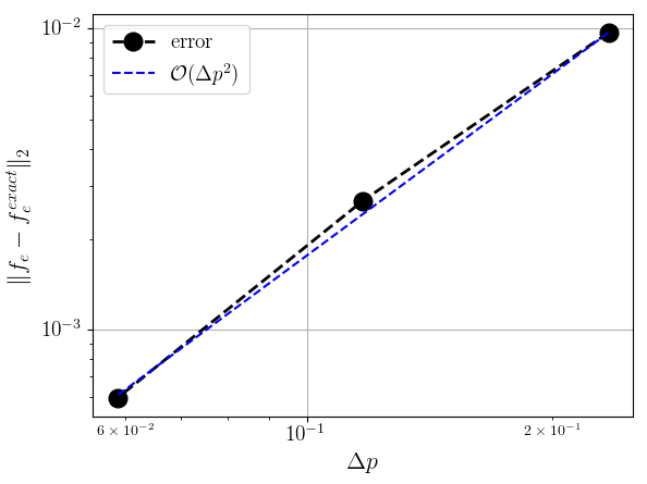

Figure 12) illustrates the spatial accuracy of the proposed scheme with the boosted MJ collisional relaxation problem described in 5.2.1. The ‘exact’ electron distribution is obtained at (before steady-state is reached) with , and , while the three data points (solid dots) correspond to coarser grids of , and . The blue dashed line corresponds to a second-order error scaling. The norm of the error between the ‘exact’ and numerical electron distributions is computed as:
We confirm that the proposed implementation is second-order accurate in space.
Figure 12) illustrates the temporal accuracy of the implementation. In this case, the ’exact’ electron distribution is obtained in a grid using the BDF2 time advancement scheme with , see description in 3.3. The four data points correspond to larger time steps of and . The proposed implementation is confirmed to be second-order accurate in time.
6 Conclusions
We have developed a fully implicit, nearly optimal, relativistic nonlinear Fokker-Plank algorithm with strict conservation properties.. We consider a 0D2P cylindrical momentum-space representation. The solver employs the differential form of the Fokker-Planck equation, which requires the solution of five relativistic potentials in momentum space to obtain the collisional coefficients. Singularities in the potential integral formulations are resolved by expressing them in terms of complete elliptic integrals of the second and third kind. To ensure a benign scaling of the potential solves with the total number of mesh points , we employ a multigrid-preconditioned GMRES solver, and have developed an adaptive spline technique for finding far-field boundary conditions for the potentials. The adaptive spline technique results in a small additional exponent in the algorithmic scaling of . Positivity of the distribution function is ensured using a continuum-based reformulation approach [18] combined with robust positivity-preserving discretizations schemes [17]. Using an Anderson Acceleration fixed-point iteration scheme for our nonlinear solves, also preconditioned with multigrid techniques, we obtain an algorithm that overall scales as . The contribution is due to the parallel multigrid techniques employed, and the contribution is from the proposed adaptive spline technique. We have demonstrated second-order accuracy in both space and time, and characterized the performance of our parallel implementation. We have verified our solver by comparing with previous results for electrical conductivity measurements in the weak and strong electric field limits. We have demonstrated the accuracy of conserved quantities in electron-electron collisions, with small relative errors, in number density, relativistic momentum, and energy. In addition, we have examined runaway dynamics and verified it by comparing to known results [8, 15, 16]. In future work, we will extend this method to study inhomogeneous plasmas by considering the spatial dependence of the electron distribution function.
Acknowledgements
The authors thank Z. Guo for help in verifying the algorithm and E. Hirvijoki for insightful discussions on the properties of the relativistic operator. The authors also thank C. McDevitt and X. Tang for useful inputs during the course of this project. This work was supported by the US Department of Energy through the Los Alamos National Laboratory. Los Alamos National Laboratory is operated by Triad National Security, LLC, for the National Nuclear Security Administration of U.S. Department of Energy (Contract No. 89233218CNA000001). This research used resources provided by the Los Alamos National Laboratory Institutional Computing Program.
Appendix A Discretization of operators in potential equations and collisional coefficients
A1. Linear potential equations.
The potential operator consists of Hessian and advective terms,
The terms are discretized using central differencing. The Laplacian piece is computed as:
where,
The remaining Hessian piece is computed as:
where
The advective piece is computed as:
Note the cell faced values of are found by linear averaging across cell centered values, for example and .
A2. Collisional coefficients.
Once the potentials are determined, the friction coefficients are evaluated using Eq. (4). The components of at the cell center are defined as:
The cell face values of are found by taking the average of cell-centered values. A similar discretization approach is used when evaluating the diffusion coefficient, Eq. (3) .
A3. Reformulated off-diagonal tensor diffusion terms (effective friction coefficients).
The off-diagonal diffusion coefficients are expressed as effective friction coefficients of the form and , see Eq (19). The momentum-space derivatives of at cell centers are evaluated by averaging the cell vertex values, for example:
where the cell vertex value is obtained by averaging over adjacent face-centered values:
where is added to mollify singularities. Once computed at the cell centers, the friction coefficients at the cell faces are found by linear averaging.
Appendix B Solution of singular integrals in relativistic potentials
B1. Solution of first singular integral
We seek a solution of the integral:
| (32) |
with:
We consider the case of . Note . Since , it follows that:
| (33) |
To begin, we consider the change of variable . We consider the following cases:
| , | ||||
| , |
This gives:
Solution of integral
We begin with the integral . We follow Abramowitz & Stegun [24], and consider the polynomials:
These polynomials have real roots , , . Because of Eq. (33), it is apparent that the last two roots are , and hence and do not have nested roots. In this case, one can consider the transformation to the canonical forms of the elliptic integrals by constructing the polynomial:
| (34) |
Seeking a zero discriminant for the quadratic form in gives the following value for :
| (35) | |||||
Note that these roots are real and semi-positive, since, by Eq. (33):
Also, it is clear that
| (36) |
and that:
| (37) |
Since the discriminant for Eq. (34) vanishes, it follows that the roots of are perfect squares and are given by:
| (38) |
Therefore:
| (39) | |||||
| (40) |
At this point, it is useful to point out a few properties of the roots in Eq. (38). Firstly, from Eq. (36) it follows that:
| (41) |
Secondly, from the polynomial in Eq. (34) and the properties of the quadratic equations, we can write:
| (42) |
which can be used to prove that:
| (43) |
(needed for later) as follows:
| (44) |
which can be shown to be true when noting that:
The inequality follows from Eq. (35). Finally, using Eq. (44) and the inequality above, we can also readily prove that:
| (45) |
which will be important later.
Eqs (39, 40) can be solved for and as follows:
Here:
Note that:
From the expressions of , , one can write:
Following Ref. [24], we postulate the change of variables:
Hence:
| (46) |
Here:
The result in Eq. (46) can be written as a canonical elliptic integral by considering:
| (47) |
to find:
Here, we have used the surprising property that:
which can be demonstrated by using the definition of (Eq. 38) and (Eq. 42).
Solution of integral
The solution of the integral follows a similar development, except now:
With these definitions, it can be shown that the discriminant of the combination is exactly the same, and therefore so are the solutions . However the roots in now have opposite signs:
| (48) |
and the factorization of reads:
From the expressions of , , one can write:
Following Ref. [24], we postulate the change of variables:
When postulating this change of variables, we have taken into account the fact that (Eq. 45), and that (Eq. 43). It follows that:
| (49) |
where:
As before, one can readily prove that:
and therefore . There results:
| (50) |
Solution of total integral
B2. Solution of second singular integral
In the previous section, we determined the root structure of the radicand and removed the odd terms in the radicand. We employ this approach and also use ideas from Ref. [25] to express the following elliptic integral,
in terms of Legendre’s elliptic functions. Recall that
The integral can thus be expressed as,
We can regroup as we know from B1 the solution when the numerator is unity,
| (51) |
Removing the odd terms in the radicand, we obtain,
and
The rational functions of , and , can be expressed in terms of odd and even functions. This is because the odd term can be simplified into elementary functions via trigonometric substitutions, see Ref. [25].
However, in our case we observe that these terms cancel each other. Examining the odd terms in and , and adding together their contribution to , we find:
as the odd function is asymmetric about the origin. The even term can be further factorized into:
Putting the above expression into and , the contributions of the even terms may be expressed as,
Simplifying and regrouping, we obtain the expression for H, see Eq. (51) as,
| (52) |
where is the complete elliptic integral of the third kind, with . This formula has been verified numerically. Also in the above, we made use of the following step which was described earlier in the previous section. It is as follows,
Then substituting to get the final form (52). The complete elliptic integral of the third kind is given by,
References
- [1] ST Beliaev and GI Budker. The relativistic kinetic equation. In Soviet Physics Doklady, volume 1, page 218, 1956.
- [2] Marshall N Rosenbluth, William M MacDonald, and David L Judd. Fokker-planck equation for an inverse-square force. Physical Review, 107(1):1, 1957.
- [3] Bastiaan J Braams and Charles FF Karney. Conductivity of a relativistic plasma. Physics of Fluids B: Plasma Physics, 1(7):1355–1368, 1989.
- [4] Adam Stahl, Matt Landreman, O Embréus, and Tünde Fülöp. Norse: A solver for the relativistic non-linear fokker–planck equation for electrons in a homogeneous plasma. Computer Physics Communications, 212:269–279, 2017.
- [5] RW Harvey, VS Chan, SC Chiu, TE Evans, MN Rosenbluth, and DG Whyte. Runaway electron production in diii-d killer pellet experiments, calculated with the cql3d/kprad model. Physics of Plasmas, 7(11):4590–4599, 2000.
- [6] Y Petrov and R W Harvey. Benchmarking the fully relativistic collision operator in CQL3D. CompX report CompX-2009-1, 2009.
- [7] Leslie Colin Woods. Theory of tokamak transport: new aspects for nuclear fusion reactor design. John Wiley & Sons, 2006.
- [8] JW Connor and RJ Hastie. Relativistic limitations on runaway electrons. Nuclear fusion, 15(3):415, 1975.
- [9] William T Taitano, Luis Chacón, AN Simakov, and K Molvig. A mass, momentum, and energy conserving, fully implicit, scalable algorithm for the multi-dimensional, multi-species rosenbluth–fokker–planck equation. Journal of Computational Physics, 297:357–380, 2015.
- [10] Bastiaan J Braams and Charles FF Karney. Differential form of the collision integral for a relativistic plasma. Physical review letters, 59(16):1817, 1987.
- [11] Eero Hirvijoki. Conservative finite-element method for the relativistic coulomb collision operator. arXiv preprint arXiv:1903.07403, 2019.
- [12] Takashi Shiroto and Yasuhiko Sentoku. Structure-preserving strategy for conservative simulation of relativistic nonlinear landau–fokker–planck equation. arXiv preprint arXiv:1902.07866, 2019.
- [13] Youcef Saad and Martin H Schultz. Gmres: A generalized minimal residual algorithm for solving nonsymmetric linear systems. SIAM Journal on scientific and statistical computing, 7(3):856–869, 1986.
- [14] Rick Beatson and Leslie Greengard. A short course on fast multipole methods. Wavelets,multilevel methods and elliptic PDEs, 1:1–37, 1997.
- [15] J Decker, E Hirvijoki, O Embreus, Y Peysson, A Stahl, I Pusztai, and T Fülöp. Numerical characterization of bump formation in the runaway electron tail. Plasma Physics and Controlled Fusion, 58(2):025016, 2016.
- [16] Zehua Guo, Christopher J McDevitt, and Xian-Zhu Tang. Phase-space dynamics of runaway electrons in magnetic fields. Plasma Physics and Controlled Fusion, 59(4):044003, 2017.
- [17] PH Gaskell and AKC Lau. Curvature-compensated convective transport: Smart, a new boundedness-preserving transport algorithm. International Journal for numerical methods in fluids, 8(6):617–641, 1988.
- [18] Erasmus J Du Toit, Martin R O‘Brien, and Roddy GL Vann. Positivity-preserving scheme for two-dimensional advection–diffusion equations including mixed derivatives. Computer Physics Communications, 228:61–68, 2018.
- [19] Donald G Anderson. Iterative procedures for nonlinear integral equations. Journal of the ACM (JACM), 12(4):547–560, 1965.
- [20] Homer F Walker and Peng Ni. Anderson acceleration for fixed-point iterations. SIAM Journal on Numerical Analysis, 49(4):1715–1735, 2011.
- [21] L Chacón, DC Barnes, DA Knoll, and GH Miley. An implicit energy-conservative 2d fokker–planck algorithm: Ii. jacobian-free newton–krylov solver. Journal of Computational Physics, 157(2):654–682, 2000.
- [22] Youcef Saad and Martin H Schultz. Gmres: A generalized minimal residual algorithm for solving nonsymmetric linear systems. SIAM Journal on scientific and statistical computing, 7(3):856–869, 1986.
- [23] SM Weng, Zheng-Ming Sheng, MQ He, J Zhang, PA Norreys, M Sherlock, and APL Robinson. Plasma currents and electron distribution functions under a dc electric field of arbitrary strength. Physical review letters, 100(18):185001, 2008.
- [24] Milton Abramowitz and Irene A Stegun. Handbook of mathematical functions: with formulas, graphs, and mathematical tables, volume 55. Courier Corporation, 1965.
- [25] George Labahn and Mark Mutrie. Reduction of elliptic integrals to legendre normal form. University of Waterloo, Computer Science Department, 1997.