Numerical simulation of a coupled system of Maxwell equations and a gas dynamic modelJournal: arXiv

The governing equations for the propagation of electromagnetic fields are the Maxwell equations

Here, ${\epsilon}_{0},{\mu}_{0}$ are the permittivity and the permeability in free space, respectively, $\tilde{\mathbf{E}}=\tilde{\mathbf{E}}^{i}+\tilde{\mathbf{E}}^{s}$ and $\tilde{\mathbf{H}}=\tilde{\mathbf{H}}^{i}+\tilde{\mathbf{H}}^{s}$ are the total fields, with $\tilde{\mathbf{E}}^{i}$ and $\tilde{\mathbf{H}}^{i}$ being the incident fields, and $\tilde{\mathbf{E}}^{s}$ and $\tilde{\mathbf{H}}^{s}$ being the scattered fields satisfying the Silver-M$\ddot{u}$ller radiation condition

where $\tilde{\mathbf{J}}$ denotes the current density generated by the motion of electrons in a metallic nanostructure and thus identically equals to zero outside the metallic nanostructure, and $\mathbf{\tilde{J}}_{b}$ is the bound current density which is trivial if the effect of bound electrons is neglected. In this paper, we take an assumption of $z$-invariance, and therefore the following notation for the curl operator is used for the vector field $\mathbb{u}=(u_{x},u_{y},u_{z})$:

As being shown in Figure 1, $\Omega_{2}\subset\mathbb{R}^{2}$ is a bounded domain occupied by a metallic nanostructure, which is excited by an external electromagnetic field with the electric field $\tilde{\mathbf{E}}(\tilde{\mathbf{x}},\tilde{t})$ and the magnetic field $\tilde{\mathbf{H}}(\tilde{\mathbf{x}},\tilde{t})$. On the other hand, the infinite mass of the ions in metal is further assumed, and it implies that the ions density $\tilde{n}_{0}(\bm{x})$ is a time independent function. Therefore, the positively charged ions merely play a role in providing background for the motion of electrons without making any contribution to the current density.

As a result, in terms of continuum mechanics, the motion of free electrons in the metallic nanostructure $\Omega_{2}$ satisfies the following Euler equations

where $\tilde{q}_{e},\tilde{m}_{e},\tilde{n}_{e},\tilde{\mathbf{u}}_{e}$ denote the electron charge, mass, number density and velocity field, respectively. $\tilde{\gamma}=1/\tilde{\tau}$ denotes the relaxation time, the average time of collisions between the electrons and the ions. $\tilde{p}={(3\pi^{2})}^{2/3}(\hbar^{2}/5\tilde{m}_{e})\tilde{n}_{e}^{5/3}$, with $\hbar$ being the Planck’s constant, is the electron gas pressure evaluated by the Thomas-Fermi theory [20]. In this work, we term the equations (1)-(5) as the modified nonlinear hydrodynamic Drude (MNHD) model. Since the coupling MNHD system is a self-consistent model with strong nonlinearity and diffusion effects, one expects to be able to observe both the high-order harmonic generation and the nonlocal optical response in numerics using this model.

Let $\Omega_{3}\subset\mathbb{R}^{2}$ (see Figure 1) be a bounded domain filled with some kind of non-metallic material, being adjacent to $\Omega_{2}$. In the domain $\Omega_{3}$, the electrons are subject to the linear and nonlinear restoring forces and can not leave far away from their atomic nucleus. We call these electrons as the bound electrons. Let $\mathbf{\tilde{P}}$ be the polarization and $\mathbf{\tilde{J}}_{b}$ be the bound current density, respectively, an effective polarization model for bound charges can be obtained by using Newton’s second law and neglecting the nonlinear restoring forces [22]

Here, $\tilde{n}_{b}$, $\tilde{\gamma}_{b}$, $\tilde{\omega}_{b}$ denote the constant ion density, damping coefficient and resonance frequency for the bound electrons, respectively, and ${c}$ denotes the speed of light in vacuum. We point out that this model defined on the domain $\Omega_{3}$ is coupled with the MNHD model for the numerical simulation only when we consider the numerical test on the influence of bound electrons (the last part in Section 4.2).

Assume that $\Omega_{1}\subset\mathbb{R}^{2}$ is a finite truncation such that $(\Omega_{2}\cup\Omega_{3})\subset\Omega_{1}$. Defining the charge density $\tilde{\rho}$ and the current density $\tilde{\mathbf{J}}$ as follows

we can write the equations (1)-(2) and (4)-(5) in the following compact hyperbolic system after a nondimensionalization procedure according to Table 1

where $\bm{F}_{1}(U_{1})=\left(F_{1}(U_{1}),G_{1}(U_{1})\right)$, $\bm{F}_{2}(U_{2})=\left(F_{2}(U_{2}),G_{2}(U_{2})\right)$. We could also formulate the polarization model into the following compact ordinary differential system according to Table 1

In the above formulations,

$T$ is the final simulation time, and the subscript $x$ ($y$ or $z$) denotes the $x$ ($y$ or $z$) component of corresponding unknowns. Finally, we indicate that the radiation condition (3) will be replaced with an approximate boundary condition on the boundary $\partial\Omega_{1}$, which is to be discussed in the next section.

We start introducing the schemes with the first order forward Euler method for the time discretization, and the higher order time discretization will be discussed in Section 3.2. The proposed schemes evolve the numerical solutions $U_{1h}$, $U_{2h}$ and $U_{3h}$, which are assumed to be available at $t=t^{n}$, denoted by $U_{1h}^{n}\in V_{h,\Omega_{1}}^{6}$, $U_{2h}^{n}\in W_{h,\Omega_{2}}^{4}$ and $U_{3h}^{n}\in V_{h,\Omega_{3}}^{6}$, and will be computed at $t=t^{n+1}=t^{n}+\Delta t^{n}$, denoted by $U_{1h}^{n+1}$, $U_{2h}^{n+1}$ and $U_{3h}^{n+1}$.

In the previous subsection, we have discussed the first order time discretization. To increase the accuracy in the time domain, strong stability preserving (SSP) high-order time discretizations [8] can be used, and we employ the third order TVD Runge-Kutta method [6] for the time discretization in this work.

Numerical investigations on complex optical phenomena are significantly correlated with numerical settings. In this subsection, we will describe in details numerical ingredients, including the initial conditions, and the interface and absorbing boundary conditions, etc..

We start with a manufactured example to study the accuracy of our schemes for MNHD model. For simplicity, we choose $k=0,\frac{q_{e}}{m_{e}}=1,\gamma=1$ in the equations (8) and (9) and employ the following as the manufactured solutions

where $\alpha=\frac{\sqrt{2}}{2}$. The computational domain is $\Omega_{2}=\Omega_{1}=[0,1]\times[0,1]$. Periodic boundary conditions are applied in both $x-$ and $y-$directions. In Table 2, we present the $L^{2}$ errors and the corresponding order of accuracy for $\rho$, $H_{z}$, $E_{x}$ and $E_{y}$ at $T=0.2$. It shows that the orders of accuracy are optimal for both $P^{k}$ solutions with $k=1,2$.

The high-order harmonic generation is a nonlinear optical process sensitive to the configurations of metallic nanostructures. In this test, we simulate the high-order harmonic generation from two typical metallic nanostructures, namely, an array of rectangular nanostructures (see the left of Figure 6) and an array of L-shaped nanostructures (see the middle of Figure 6). In addition, we also consider an array of L-shaped nanostructures with metallic materials and an array of rectangular nanostructures with non-metallic materials (see the right of Figure 6) for purpose of studying the influence of bound electrons on the generation of high order harmonic waves. In our simulations, the nanostructures are arranged periodically in $x-$direction with plasma frequency ${\omega}_{p}=4.560\times 10^{-2}$, and ${\gamma}=2.160\times 10^{-4}$. For simplicity, we only focus on one single structure by using periodic boundary condition in $x-$direction and PML in $y-$direction [16]. Measurements on the linear response and the SHG signal can be computed in terms of the integrals of the electric fields $E_{z}$ and $E_{x}$ along the probing line $S$ as follows

We employ an uniform mesh $\Delta x=\Delta y=2.0$ in the simulation and the final time $T=1.499\times 10^{5}$.

Firstly, we study the high order harmonic generation from the rectangular metallic nanostructures whose dimension is shown in Figure 6 (Left). In Figure 7, we plot the time history of linear response and SHG. As being shown in Figure 7, there is no SHG from the rectangular metallic particle. This result is reasonable since the rectangular metallic nanostructure possesses a perfect centrosymmetric property which leads to a vanishing second-order nonlinear optical susceptibility tensor $\chi^{(2)}$ prohibiting the SHG. However, the rectangular metallic nanostructure does allow for the third harmonic generation (THG) since the symmetric property would not remove the third-order nonlinear optical susceptibility tensor $\chi^{(3)}$. In Figure 8 (Left), spectrums of these responses are presented. In order to show the spectrums apparently, a zoom-in plot of the spectrum is presented in Figure 8 (Right). It can be observed that, the third-order harmonic generation ($400$), the fifth-order harmonic generation ($240$) and the seventh-order harmonic generation ($171.4$) are captured in the simulation. These figures also indicate that, apart from the nonlinear optical responses, the MNHD model maintains the description of the linear optical interaction.

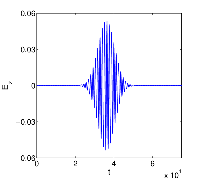
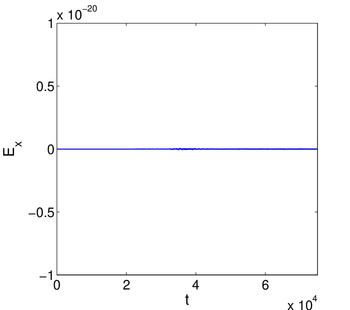
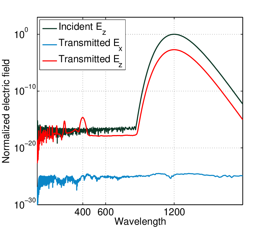
Then, we take an investigation on the high order harmonic generation from the L-shaped metallic nanostructures (see Figure 6 (middle) for the setup). In Figure 9, we plot the time history of the linear response and the SHG. In Figure 10 (Left), spectrums of these responses are presented. Since the centrosymmetry is broken in this case, the second order harmonic generation appears. As we can see from Figure 10 that the fundamental wave ($1200$) can be frequency-doubled after propagating through the nanostructure, and the higher order harmonic waves, such as the third-order harmonic generation ($400$), the fifth-order harmonic generation ($240$) and the seventh-order harmonic generation ($171.4$) in the transmitted $E_{z}$, are also captured in the simulation. The above results associated with both the rectangular and the L-shaped metallic nanostructures are in a good agreement with those presented in [16].

Finally, we investigate the high order harmonic generation from an L-shaped metallic nanostructure, with a rectangular non-metallic material occupied nanostructure being located at its corner (see the right of Figure 6), to study the influence of bound electrons on the generation of high order harmonic waves. The simulation setting is the same as the L-shaped case. In the simulations, we make a selection as ${n}_{b}=58.0$, ${\omega}_{b}=\sqrt{{n}_{b}{q}_{e}^{2}/{m}_{e}}$, ${\gamma}_{b}=0.8{\gamma}$. In Figure 11 (Left), spectrums of the linear and nonlinear optical responses are presented, in comparison with spectrums obtained from the L-shaped metallic nanostructure in the previous test. It can be observed that the high-order harmonics are enhanced when the interaction between the bound electrons and the external electromagnetic waves has been taken into account.

For small optical particles, especially for particles with size down to subwavelength, apart from the surface plasmon, the bulk plasmon could be excited as well. In this test, we solve the MNHD model to investigate the nonlocal effect for the Ag nanowire. As in [10], we choose the nanowire with radius ${r}=2.0$, the plasma frequency ${\omega}_{p}=2.885\times 10^{-2}$, and the damping constant ${\gamma}=0.01{\omega}_{p}$. PML boundary conditions are employed in both $x-$ and $y-$directions. To resolve the ECS in the time domain, we introduce the $x-$polarized incident wave propagating in $y-$direction by the TF/SF technique and collect the Fourier-transformed total field and scattered field on the TF/SF boundary. The ECS is calculated as follows

where $\mathbf{n}$ denotes the outward unit normal to the TF/SF boundary $F$, and $\mathbf{S}_{\vartriangle}$ denotes the time averaged Poynting vector

We try to recover the normalized ECS from $0.4{\omega}_{p}$-$1.4{\omega}_{p}$ [10]. In the simulations, we adopt a short Gaussian pulse with ${t}_{b}=2.998,~{\lambda}_{0}=300$ carrying effective information between the range $0.4{\omega}_{p}$-$1.4{\omega}_{p}$ to perform a broad-band calculation. We simulate the optical interaction for a long time such that the scattered field decays adequately into a steady state and we set the final time ${T}=5.996\times 10^{4}$ for this purpose. In Figure 12, we present the ECS being normalized with respect to the diameter of nanowire as a function of the normalized angular frequency $\omega/\omega_{p}$. It can be seen from Figure 12 that the bulk plasmon resonances beyond the plasma frequency can be excited with the MNHD model. A slight blue-shift (from $\omega/\omega_{p}=0.703$ to $\omega/\omega_{p}=0.714$) of the surface plasmon resonance has been retrieved in the ECS as well. In order to make a further exploration on the source for the appearance of bulk plasmon resonances, we switch off the different nonlinear terms (quantum pressure term: $k\rho^{5/3}$, convection terms: $\rho u_{i}u_{j},i,j=x,y,z$, magnetic terms: $u_{i}H_{j}-u_{j}-H_{i},(i,j)=(x,y),(y,z),(z,x)$) in the equation (9), and make the calculation of the ECS, respectively. It can be observed from Figure 12 that, apart from the ECS calculated from the MNHD model without the quantum pressure term, all other ECSs are in perfect match with the calculated ECSs associated to the full MNHD model. This indicates that, among all three terms, the quantum pressure makes a unique contribution to appearance of the nonlocal effect. In Figure 13, we provide with the Fourier-transformed current density at $\omega/\omega_{p}=1.1835$. As it is shown, the resonances, namely the bulk plasmon, get excited in the bulk of nanowire.

References

- [1] J. N. Anker, W. P. Hall, O. Lyandres, N. C. Shah, J. Zhao, R. P. Van Duyne, Biosensing with Plasmonic Nanosensors, Nat. Mater., 7 (2008) 442-453 .
- [2] V. A. Bokil, Y. Cheng, Y. Jiang, F. Li, Energy stable discontinuous Galerkin methods for Maxwell’s equations in nonlinear optical media, J. Comput. Phys., 350 (2017) 420-452.
- [3] S. I. Bozhevolnyi, V. S. Volkov, E. Devaux, J.-Y. Laluet, T. W. Ebbesen, Channel plasmon subwavelength waveguide components including interferometers and ring resonators, Nature, 440 (2006) 508-511.
- [4] X. Chen, O. Nadiarynkh, S. Plotnikov, P. J. Campagnola, Second harmonic generation microscopy for quantitative analysis of collagen fibrillar structure, Nat. Protoc., 7 (2012) 654-669.
- [5] C. Ciraci, R.T. Hill, J.J. Mock, Y. Urzhumov, A.I. Fernandez-Dominquez, S.A. Maier, J.B. Pendry, A. Chilkoti, D.R. Smith, Probing the ultimate limits of plasmonic enhancement, Science, 337 (2012) 1072-1074.
- [6] B. Cockburn, C.-W. Shu, The Runge-Kutta discontinuous Galerkin method for conservation laws V: multidimensional systems, J. Comput. Phys., 141 (1998) 199-224.
- [7] M. Fang, Z. Huang, W. E. I. Sha, X. Xiong, X. Wu, Full hydrodynamic model of nonlinear electromagnetic response in metallic metamaterials, Prog. Electromagn. Res. 157 (2016) 63.
- [8] S. Gottlieb, C.-W. Shu, E. Tadmor, Strong stability preserving high order time discretization methods, SIAM Review, 43 (2001) 89-112.
- [9] A. Hille, M. Moeferdt, C. Wolff, C. Matyssek, R. Rodríguez-Oliveros, C. Prohm, J. Niegemann, S. Grafström, L.M. Eng, K. Busch, Second harmonic generation from metal nano-particle resonators: Numerical analysis on the basis of the hydrodynamic Drude model, J. Phys. Chem. C, 120 (2016) 1163-1169.
- [10] K. R. Hiremath, L. Zschiedrich, F. Schmidt, Numerical solution of nonlocal hydrodynamic Drude model for arbitrary shaped nano-plasmonic structures using Nédélec finite elements, J. Comput. Phys., 231 (2012) 5890-5896.
- [11] J. D. Jackson, Classical Electrodynamics, 3rd ed., Wiley (1999).
- [12] M. W. Klein, C. Enkrich, M. Wegener, S. Linden, Second-harmonic generation from magnetic metamaterials, Science, 313 (2006) 502-504.
- [13] M. W. Klein, M. Wegener, N. Feth, S. Linden, Experiments on second- and third-harmonic generation from magnetic metamaterials, Opt. Express, 15 (2007) 5238-5247.
- [14] A. V. Krasavin, P. Ginzburg, G. A. Wurtz, A.V. Zayats, Nonlocality-driven supercontinuum white light generation in plasmonic nanostructures, Nat. Commum. 7 (2016) 11497.
- [15] S. Lal, S. E. Clare, N. J. Halas, Nanoshell-enabled photothermal cancer therapy: impending clinical impact, Acc. Chem. Res., 41 (2008) 1842-1851.
- [16] J. Liu, M. Brio, Y. Zeng, A. R. Zakharian, W. Hoyer, S. W. Koch, J. V. Moloney, Generalization of the FDTD algorithm for simulations of hydrodynamic nonlinear Drude model, J. Comput. Phys., 229 (2010) 5921-5932.
- [17] T. Lu, P. Zhang, W. Cai, Discontinuous Galerkin methods for dispersive and lossy Maxwell¡¯s equations and PML boundary conditions, J. Comput. Phys., 200 (2004) 549-580.
- [18] N.A. Mortensen, S. Raza, M. Wubs, T. Sondergaard, S.I. Bozhevolnyi, A generalized non-local optical response theory for plasmonic nanostrutures, Nat. Commun., 5 (2014) 3809.
- [19] F. B. P. Niesler, N. Feth, S. Linden, J. Niegemann, J. Gieseler, K. Busch, M. Wegener, Second-harmonic generation from split-ring resonators on a GaAs substrate, Opt. Lett., 34 (2009) 1997-1999.
- [20] R. G. Parr, W. Yang, Density-Functional Theory of Atoms and Molecules, Oxford Univ. Press, 1994.
- [21] C. K. N. Patel, Efficient Phase-Matched Harmonic Generation in Tellurium with a Laser at , Phys. Rev. Lett., 15 (1965) 1027-1030.
- [22] M. Scalora, M. A. Vincenti, D. de Ceglia, V. Roppo, M. Centini, N. Akozbek, M. J. Bloemer, M. Centini, Second and Third Harmonic Generation in Metal-Based Nanostructures, Phys. Rev. A, 82 (4) (2010) 5929-5937.
- [23] N. Schmitt, C. Scheid, S. Lanteri, A. Moreau, J. Viquerat, A DGTD method for the numerical modeling of the interaction of light with nanometer scale metallic structures taking into account non-local dispersion effects, J. Comput. Phys., 316 (2016) 396-415.
- [24] H. Sonnenberg, H. Heffner, Experimental Study of optical second-harmonic generation in silver, J. Opt. Soc. Am., 58 (1968) 209-212.
- [25] A. Taflove, Computational Electrodynamics: The Finite-Difference Time-Domain Method, Artech House, London, 1995.
- [26] G. Toscano, J. Straubel, A. Kwiatkowski, C. Rockstuhl, F. Evers, H. Xu, N. A. Mortensen, M. Wubs, Resonance shifts and spill-out effects in self-consistent hydrodynamic nanoplasmonics, Nat. Commun., 6 (2015) 7312.
- [27] F. Vidal-Codina, N. C. Nguyen, S.-H. Oh, J. Peraire, A hybridizable discontinuous Galerkin method for computing nonlocal electromagnetic effects in three-dimensional metallic nanostructures, J. Comput. Phys., 355 (2018) 548-565.
- [28] P. Wasylczyk, I. A. Walmsley, W. Wasilewski, C. Radzewicz, Broadband noncollinear optical parametric amplifier using a single crystal, Opt. Lett., 30 (2005) 1704-1706.
- [29] Y. Zeng, W. Hoyer, J. Liu, S.W. Koch, J.V. Moloney, A classical theory for second-harmonic generation from metallic nanoparticles, Phys. Rev. B, 79 (2009) 235109.