跳到论文正文
W Papers独立论文阅读器 arXiv:1902.09772 论文正文 计算阅读时间 · 0%
引用这篇论文根据当前论文元数据生成,正式投稿前建议核对。


License: arXiv.org perpetual non-exclusive license
arXiv:1902.09772v2 [math.AP] 01 Aug 2019

Asymptotic stability of shock profiles and rarefaction waves under periodic perturbations for 1-d convex scalar viscous conservation lawsThanks: This research is partially supported by Zheng Ge Ru Foundation, Hong Kong RGC Earmarked Research Grants, CUHK-14300917, CUHK-14305315, and CUHK-14302917. Thanks: The research of Yuan Yuan is also supported by the Start-up Research Grant of South China Normal University (8S0328).

Zhouping XIN Z. XinThe Institute of Mathematical Sciences & Department of Mathematics, The Chinese University of Hong Kong, Shatin, N.T., Hong Kong Email address: zpxin@ims.cuhk.edu.hk , Qian YUAN Q. YuanThe Institute of Mathematical Sciences & Department of Mathematics, The Chinese University of Hong Kong, Shatin, N.T., Hong Kong Email address: qyuan103@link.cuhk.edu.hk and Yuan YUAN Y. YuanSouth China Research Center for Applied Mathematics and Interdisciplinary Studies, South China Normal University, Guangzhou, Guangdong, China Email address: yyuan2102@m.scnu.edu.cn
Abstract.

This paper studies the asymptotic stability of shock profiles and rarefaction waves under space-periodic perturbations for one-dimensional convex scalar viscous conservation laws. For the shock profile, we show that the solution approaches the background shock profile with a constant shift in the L∞​(ℝ)L^{\infty}(\mathbb{R}) norm at exponential rates. The new phenomena contrasting to the case of localized perturbations is that the constant shift cannot be determined by the initial excessive mass in general, which indicates that the periodic oscillations at infinities make contributions to this shift. And the vanishing viscosity limit for the shift is also shown. The key elements of the poof consist of the construction of an ansatz which tends to two periodic solutions as x→±∞,x\rightarrow\pm\infty, respectively, and the anti-derivative variable argument, and an elaborate use of the maximum principle. For the rarefaction wave, we also show the stability in the L∞​(ℝ)L^{\infty}(\mathbb{R}) norm.

1. Introduction and main results

We consider the Cauchy problem for one-dimensional convex scalar viscous conservation laws

(1.1) ∂tuν+∂xf⁡(uν)\displaystyle\partial_{t}u^{\nu}+\partial_{x}f(u^{\nu}) =ν​∂x2uν,x∈ℝ,t>0,\displaystyle=\nu\partial_{x}^{2}u^{\nu},\qquad x\in\mathbb{R},~t>0,
(1.2) uν​(x,0)\displaystyle u^{\nu}(x,0) =u0​(x),x∈ℝ,\displaystyle=u_{0}(x),\qquad x\in\mathbb{R},

where uν​(x,t)∈ℝu^{\nu}(x,t)\in\mathbb{R} is the unknown, the flux ff is smooth and strictly convex, and ν∈(0,1]\nu\in(0,1] denotes the viscosity. This paper is concerned with the asymptotic behavior of the solution uν​(x,t)u^{\nu}(x,t) to (1.1), (1.2) with u0​(x)∈L∞​(ℝ)u_{0}(x)\in L^{\infty}(\mathbb{R}) satisfying

(1.3) {|u0​(x)−u¯l−w0​l​(x)|≤C0​eβ0​x,|u0​(x)−u¯r−w0​r​(x)|≤C0​e−β0​x,x∈ℝ,\begin{cases}|u_{0}(x)-\overline{u}_{l}-w_{0l}(x)|\leq C_{0}e^{\beta_{0}x},&\\ |u_{0}(x)-\overline{u}_{r}-w_{0r}(x)|\leq C_{0}e^{-\beta_{0}x},&\end{cases}\quad x\in\mathbb{R},

where u¯l,u¯r,C0>0\overline{u}_{l},\overline{u}_{r},C_{0}>0 and β0>0\beta_{0}>0 are constants, and w0​l,w0​r∈L∞​(ℝ)w_{0l},w_{0r}\in L^{\infty}(\mathbb{R}) are two arbitrary periodic functions.

It is well known from [28, 20] that for ν>0,\nu>0, the equation (1.1) generates a semi-group {Stν:L∞(ℝ)→L∞(ℝ);t≥0}\{S_{t}^{\nu}:L^{\infty}(\mathbb{R})\rightarrow L^{\infty}(\mathbb{R});t\geq 0\} to ensure that, for any initial data u0∈L∞​(ℝ)u_{0}\in L^{\infty}(\mathbb{R}), the function uν​(x,t):=Stν​u0u^{\nu}(x,t):=S_{t}^{\nu}u_{0} is the unique bounded solution to (1.1), Equation 1.2, which is smooth for t>0,t>0, and satisfies the initial condition in the weak sense: for any continuous functions φ⁡(x,t)\varphi(x,t) compactly supported in ℝ×[0,+∞),\mathbb{R}\times[0,+\infty), there holds

∫ℝ[φ⁡(x,t)​uν​(x,t)−φ⁡(x,0)​u0​(x)]​𝑑x→0as​t→0.\int_{\mathbb{R}}[\varphi(x,t)u^{\nu}(x,t)-\varphi(x,0)u_{0}(x)]\ dx\rightarrow 0\quad\text{as}~t\rightarrow 0.

The semi-group StνS_{t}^{\nu} satisfies the following classical Co-properties:

  • •

    (Comparison) If u0,v0∈L∞​(ℝ)u_{0},v_{0}\in L^{\infty}(\mathbb{R}) and u0≤v0u_{0}\leq v_{0} almost everywhere, then Stν​u0≤Stν​v0S_{t}^{\nu}u_{0}\leq S_{t}^{\nu}v_{0} for any x∈ℝ,t>0.x\in\mathbb{R},~t>0.

  • •

    (Contraction) If u0,v0∈L∞​(ℝ)u_{0},v_{0}\in L^{\infty}(\mathbb{R}) and u0−v0∈L1​(ℝ)u_{0}-v_{0}\in L^{1}(\mathbb{R}), then Stν​u0−Stν​v0∈L1​(ℝ)S_{t}^{\nu}u_{0}-S_{t}^{\nu}v_{0}\in L^{1}(\mathbb{R}) and ‖Stν​u0−Stν​v0‖L1​(ℝ)\|S_{t}^{\nu}u_{0}-S_{t}^{\nu}v_{0}\|_{L^{1}(\mathbb{R})} is non-increasing with respect to t.t.

  • •

    (Conservation) If u0,v0∈L∞​(ℝ)u_{0},v_{0}\in L^{\infty}(\mathbb{R}) and u0−v0∈L1​(ℝ)u_{0}-v_{0}\in L^{1}(\mathbb{R}), then

    ∫ℝ(Stν​u0−Stν​v0)​𝑑x=∫ℝ(u0−v0)​𝑑x∀t≥0.\int_{\mathbb{R}}(S_{t}^{\nu}u_{0}-S_{t}^{\nu}v_{0})dx=\int_{\mathbb{R}}(u_{0}-v_{0})dx\qquad\forall~t\geq 0.

Moreover, there exists a constant E>0,E>0, depending only on ff and ‖u0‖L∞,\|u_{0}\|_{L^{\infty}}, such that

(1.4) ∂xuν​(x,t)≤Et∀x∈ℝ,t>0.\partial_{x}u^{\nu}(x,t)\leq\frac{E}{t}\qquad\forall x\in\mathbb{R},~t>0.

Shocks and rarefaction waves are most important nonlinear solutions to conservation laws. A viscous shock profile ϕν​(x−s​t)\phi^{\nu}(x-st) is a classical traveling wave solution to the viscous conservation law (1.1), solving the problem:

(1.5) {ν​(ϕν)′′=f′​(ϕν)​(ϕν)′−s​(ϕν)′,limx→−∞ϕν(x)=u¯l,limx→+∞ϕν(x)=u¯r,\begin{cases}&\nu(\phi^{\nu})^{\prime\prime}=f^{\prime}(\phi^{\nu})(\phi^{\nu})^{\prime}-s(\phi^{\nu})^{\prime},\\ &\lim\limits_{x\rightarrow-\infty}\phi^{\nu}(x)=\overline{u}_{l},~\lim\limits_{x\rightarrow+\infty}\phi^{\nu}(x)=\overline{u}_{r},\end{cases}

where u¯l>u¯r\overline{u}_{l}>\overline{u}_{r} and ss is the shock speed defined by the Rankine-Hugoniot condition:

s=f⁡(u¯l)−f⁡(u¯r)u¯l−u¯r.s=\dfrac{f(\overline{u}_{l})-f(\overline{u}_{r})}{\overline{u}_{l}-\overline{u}_{r}}.

The existence of the shock profile follows from a simple phase plane analysis, and can also follow from the center-manifold theorem in Kopell-Howard [18]. For u¯l<u¯r,\overline{u}_{l}<\overline{u}_{r}, a centered rarefaction wave

uR​(x,t)={u¯l,xt<f′​(u¯l),(f′)−1​(xt),f′​(u¯l)≤xt≤f′​(u¯r),u¯r,xt>f′​(u¯r),u^{R}(x,t)=\begin{cases}\overline{u}_{l},&\quad\frac{x}{t}<f^{\prime}(\overline{u}_{l}),\\ (f^{\prime})^{-1}(\frac{x}{t}),&\quad f^{\prime}(\overline{u}_{l})\leq\frac{x}{t}\leq f^{\prime}(\overline{u}_{r}),\\ \overline{u}_{r},&\quad\frac{x}{t}>f^{\prime}(\overline{u}_{r}),\end{cases}

is an entropy weak solution to the Riemann problem for the inviscid conservation law Equation 1.1 with ν=0.\nu=0.

When the initial data u0u_{0} approaches constant states as |x|→+∞,|x|\rightarrow+\infty, i.e. w0​l=w0​r=0w_{0l}=w_{0r}=0 in Equation 1.3, the asymptotic behaviors of solutions to Equation 1.1, Equation 1.2 have been studied widely so far. The pioneering work of Hopf [14] showed the L∞L^{\infty} stability of constants with a decay rate 1/t,1/\sqrt{t}, by using an explicit representation of the solution to the Burgers’ equation. Later, Il’in-Oleǐnik [16] applied the maximum principle on the anti-derivative variables to prove the L∞L^{\infty} stability of constants, shocks and rarefaction waves for general convex conservation laws. Moreover, Freistühler-Serre [5] combined a lap number argument and maximum principle to prove the L1L^{1} stability of viscous shock profiles. For more results, we refer to [27, 11, 15] for the one-dimensional scalar case, [9, 32, 12, 13, 17] for the multi-dimensional scalar case, and [26, 8, 23, 24, 31, 25, 29] for the important one-dimensional system case.

For the initial data which keeps oscillating at infinities, Lax [22] was the first one to study the periodic data. He showed that the entropy periodic solutions to inviscid scalar conservation laws approach their constant averages in the L∞L^{\infty} norm at algebraic rates. And then Glimm-Lax [7] and Dafermos [1] used the generalized characteristics to extend the results to some 2×22\times 2 systems. Besides the constants, Xin-Yuan-Yuan [33] and Yuan-Yuan [34] proved the L∞L^{\infty} stability of shocks and rarefaction waves under periodic perturbations for the scalar inviscid conservation laws, by using the generalized characteristics. One can also see [3, 4] for the L1L^{1} stability of the stationary viscous “ shock profile ” which connects two periodic functions as end states, where the flux in the equation Equation 1.1 is f⁡(x,u)f(x,u) that is periodic with respect to x.x.

In this paper, we deal with the initial data (1.3), where w0​l,w0​rw_{0l},w_{0r} are arbitrary periodic functions, in order to see how the initial oscillations at infinities influence the stability of these two nonlinear waves in the viscous case. Throughout this paper, we let ϕ⁡(x)\phi(x) denote any fixed shock profile solving Equation 1.5 with ν=1,\nu=1, and then for any ν>0,\nu>0, we define

(1.6) ϕν​(x):=ϕ​(xν).\phi^{\nu}(x):=\phi\left(\frac{x}{\nu}\right).

Then ϕν\phi^{\nu} solves Equation 1.5 for any ν>0\nu>0 and tends to the inviscid Lax-shock

uS​(x,t)={u¯l,x<s​t,u¯r,x>s​t,u^{S}(x,t)=\begin{cases}\overline{u}_{l},&\quad x<st,\\ \overline{u}_{r},&\quad x>st,\end{cases}

almost everywhere as the viscosity ν→0+.\nu\rightarrow 0+. With the constants u¯l,u¯r\overline{u}_{l},\overline{u}_{r} and periodic perturbations w0​l,w0​r∈L∞​(ℝ)w_{0l},w_{0r}\in L^{\infty}(\mathbb{R}) in Equation 1.3, we let ulν,u_{l}^{\nu}, urνu_{r}^{\nu} denote the periodic solutions to Equation 1.1 with the respective initial data

(1.7) ulν​(x,0)=u¯l+w0​l​(x),urν​(x,0)=u¯r+w0​r​(x).u_{l}^{\nu}(x,0)=\overline{u}_{l}+w_{0l}(x),\quad u_{r}^{\nu}(x,0)=\overline{u}_{r}+w_{0r}(x).

Now the main results of this paper are stated as follows:

Theorem 1.1.

Assume that ν>0\nu>0 and the initial data u0∈L∞​(ℝ)u_{0}\in L^{\infty}(\mathbb{R}) satisfies Equation 1.3 with u¯l>u¯r\overline{u}_{l}>\overline{u}_{r} and the periodic functions w0​l,w0​r∈L∞w_{0l},w_{0r}\in L^{\infty} with the respective periods pl,pr>0,p_{l},p_{r}>0, satisfying

(1.8) 1pl​∫0plw0​l​(x)​𝑑x=1pr​∫0prw0​r​(x)​𝑑x=0.\frac{1}{p_{l}}\int_{0}^{p_{l}}w_{0l}(x)dx=\frac{1}{p_{r}}\int_{0}^{p_{r}}w_{0r}(x)dx=0.

Then the unique bounded solution uνu^{\nu} to Equation 1.1, Equation 1.2 satisfies

(1.9) supx∈ℝ|uν​(x,t)−ϕν​(x−s​t−X∞ν)|≤C​e−μ​t,t>0,\sup_{x\in\mathbb{R}}\left|u^{\nu}(x,t)-\phi^{\nu}(x-st-X_{\infty}^{\nu})\right|\leq Ce^{-\mu t},\quad t>0,

with the constant shift X∞ν=1u¯l−u¯r​(X∞,1ν+X∞,2ν)X_{\infty}^{\nu}=\frac{1}{\overline{u}_{l}-\overline{u}_{r}}\left(X_{\infty,1}^{\nu}+X_{\infty,2}^{\nu}\right) given by

(1.10) X∞,1ν=\displaystyle X_{\infty,1}^{\nu}= ∫−∞0(u0−ϕν−w0​l)​(x)​𝑑x+∫0+∞(u0−ϕν−w0​r)​(x)​𝑑x,\displaystyle\int_{-\infty}^{0}(u_{0}-\phi^{\nu}-w_{0l})(x)dx+\int_{0}^{+\infty}(u_{0}-\phi^{\nu}-w_{0r})(x)dx,
(1.11) X∞,2ν=\displaystyle X_{\infty,2}^{\nu}= ∫0+∞1pl​∫0pl[f⁡(ulν​(x,t))−f⁡(u¯l)]​𝑑x​𝑑t−1pl​∫0pl∫0xw0​l​(y)​𝑑y​𝑑x\displaystyle\int_{0}^{+\infty}\frac{1}{p_{l}}\int_{0}^{p_{l}}[f(u_{l}^{\nu}(x,t))-f(\overline{u}_{l})]dxdt-\frac{1}{p_{l}}\int_{0}^{p_{l}}\int_{0}^{x}w_{0l}(y)dydx
−∫0+∞1pr∫0pr[f(urν(x,t))−f(u¯r)]dxdt+1pr∫0pr∫0xw0​r(y)dydx.\displaystyle-\int_{0}^{+\infty}\frac{1}{p_{r}}\int_{0}^{p_{r}}[f(u_{r}^{\nu}(x,t))-f(\overline{u}_{r})]dxdt+\frac{1}{p_{r}}\int_{0}^{p_{r}}\int_{0}^{x}w_{0r}(y)dydx.

1.1 shows that in contrast to the case of localized perturbations, besides the localized part of the initial perturbation, the periodic oscillations at infinities generate another shift X∞,2νX_{\infty,2}^{\nu} to the background viscous shock profile. The next theorem shows that this shift is non-zero in general even in the case the periods of the perturbations at x=±∞x=\pm\infty are the same.

Theorem 1.2.

Under the assumptions of 1.1, if w0​l=w0​r=w0,w_{0l}=w_{0r}=w_{0}, the constant X∞,2νX_{\infty,2}^{\nu} defined in Equation 1.11 may be non-zero in general. More precisely,

  1. (1)

    for the Burgers’ equation, i.e. f⁡(u)=u2/2,f(u)=u^{2}/2, it holds that X∞,2ν=0;X_{\infty,2}^{\nu}=0;

  2. (2)

    for any periodic perturbation w0w_{0} with zero average, if

    0<‖w0‖L∞​(ℝ)<(u¯l−u¯r)/2,0<\|w_{0}\|_{L^{\infty}(\mathbb{R})}<(\overline{u}_{l}-\overline{u}_{r})/2,

    there exists a smooth and strictly convex flux ff such that X∞,2ν≠0.X_{\infty,2}^{\nu}\neq 0.

However, for the inviscid conservation law Equation 1.1 with ν=0,\nu=0, it is shown in [33] that if w0​l=w0​r,w_{0l}=w_{0r}, the entropy solution u0u^{0} tends to the background shock uSu^{S} with no shift, i.e. X∞,20=0X_{\infty,2}^{0}=0 in this case. The vanishing viscosity limit for the shift X∞,2νX_{\infty,2}^{\nu} is presented in the next theorem, which agrees with the results in [33, 34].

Theorem 1.3.

Under the assumptions of 1.1, as the viscosity ν→0+,\nu\rightarrow 0+,

(1.12) X∞,2ν→X∞,20:=−min⁡∫0xx∈ℝ⁡w0​l​(y)​𝑑y+min⁡∫0xx∈ℝ⁡w0​r​(y)​𝑑y.X_{\infty,2}^{\nu}\rightarrow X_{\infty,2}^{0}:=-\min_{x\in\mathbb{R}}\int_{0}^{x}w_{0l}(y)dy+\min_{x\in\mathbb{R}}\int_{0}^{x}w_{0r}(y)dy.

Furthermore, if both w0​lw_{0l} and w0​rw_{0r} have bounded total variations on their respective periodic domains, there exists a constant C>0,C>0, independent of the viscosity ν,\nu, such that

(1.13) |X∞,2ν−X∞,20|≤C​ν1/5.\left|X_{\infty,2}^{\nu}-X_{\infty,2}^{0}\right|\leq C\nu^{1/5}.

At last, we state the result for rarefaction waves.

Theorem 1.4.

Assume that ν>0\nu>0 and the initial data u0u_{0} satisfies Equation 1.3 with u¯l<u¯r\overline{u}_{l}<\overline{u}_{r} and the periodic functions w0​l,w0​r∈L∞w_{0l},w_{0r}\in L^{\infty} with the respective periods pl,pr>0,p_{l},p_{r}>0, satisfying Equation 1.8. Then the unique bounded solution uνu^{\nu} to (1.1), (1.2) satisfies

supx∈ℝ|uν​(x,t)−uR​(x,t)|→0as​t→∞.\sup_{x\in\mathbb{R}}|u^{\nu}(x,t)-u^{R}(x,t)|\rightarrow 0~\quad\text{as}~t\rightarrow\infty.

Consequently, different from the localized perturbations, i.e., the background shock can absorb all localized perturbations on the two sides and finally tends to itself with no shift (if the perturbation has zero mass), the periodic perturbations at infinities produce infinite perturbations onto the background shock, ended up with a constant shift, which cannot be determined explicitly by the initial perturbations in the viscous case.

The main difficulty to prove 1.1 is that the perturbation uν−ϕνu^{\nu}-\phi^{\nu} is not integrable anymore, which makes it difficult to use an anti-derivative argument as before that plays an important role in the previous study of the stability under localized perturbations. In fact, if one considers the equation of the perturbation, the coefficient of the zero-order term is f′′​(ϕν)​(ϕν)′<0,f^{\prime\prime}(\phi^{\nu})(\phi^{\nu})^{\prime}<0, which makes it harder to use either the maximum principle or the energy method. One of the key elements of our proof is that we find an ansatz ψXν​(t)ν​(x,t)\psi_{X^{\nu}(t)}^{\nu}(x,t), where Xν​(t)X^{\nu}(t) is a shift function (see (2.15)) such that the difference uν−ψXν​(t)νu^{\nu}-\psi_{X^{\nu}(t)}^{\nu} is integrable and has zero mass for large time. Therefore, it is plausible to study the equation of the anti-derivative variable of the difference uν−ψXν​(t)νu^{\nu}-\psi_{X^{\nu}(t)}^{\nu} (for the Burgers’ equation, the ansatz actually coincides with the solution uνu^{\nu} at an arithmetic sequence of time {tk};\{t_{k}\}; see 2.8). We show that the limit of Xν​(t)−s​tX^{\nu}(t)-st as t→+∞t\rightarrow+\infty is actually the constant shift X∞νX_{\infty}^{\nu} in 1.1. And although the ansatz ψXν​(t)ν\psi_{X^{\nu}(t)}^{\nu} is not a solution to Equation 1.1, the error (see Equation 2.10) decays exponentially both in space and in time. Then following the idea of Il’in-Oleǐnik [16], one can construct auxiliary functions and use the maximum principle to obtain our main results.

2. Preliminaries and ansatz

We first present some useful lemmas and introduce some notations, and then construct the ansatz. Important properties of the ansatz will be stated as propositions, which will be proved in the rest of the paper. In the end of this section, we outline the organizations of the proof.

Lemma 2.1.

Assume that u0​(x)∈L∞​(ℝ)u_{0}(x)\in L^{\infty}(\mathbb{R}) is periodic with period p>0p>0 and average u¯=1p​∫0pu0​(x)​𝑑x.\overline{u}=\frac{1}{p}\int_{0}^{p}u_{0}(x)dx. Then there exists a constant α>0,\alpha>0, depending only on pp and ν,\nu, such that for any integers k,l≥0,k,l\geq 0, the periodic solution uν​(x,t)u^{\nu}(x,t) to (1.1),Equation 1.2 satisfies that

(2.1) ‖∂tk∂xl(uν−u¯)‖L∞​(ℝ)≤C​e−α​t,t≥1,\|\partial_{t}^{k}\partial_{x}^{l}(u^{\nu}-\overline{u})\|_{L^{\infty}(\mathbb{R})}\leq Ce^{-\alpha t},\quad t\geq 1,

where C>0C>0 is independent of time t.t.

The proof of 2.1 can be obtained by standard energy estimates and the Poincaré inequality, which is given in the Appendix A. Thus, there exists an α>0,\alpha>0, depending on pl,prp_{l},p_{r} and ν,\nu, such that ulνu_{l}^{\nu} and urνu_{r}^{\nu} satisfy Equation 2.1 with u¯=u¯l\overline{u}=\overline{u}_{l} and u¯r,\overline{u}_{r}, respectively.

Lemma 2.2.

Assume that u0,u~0∈L∞​(ℝ)u_{0},\tilde{u}_{0}\in L^{\infty}(\mathbb{R}) and there exist constants C>0C>0 and δ∈ℝ\delta\in\mathbb{R} such that

|u0​(x)−u~0​(x)|≤C​eδ​x,x∈ℝ.|u_{0}(x)-\tilde{u}_{0}(x)|\leq Ce^{\delta x},\quad x\in\mathbb{R}.

Then it holds that

|Stν​u0−Stν​u~0|≤C⁡(t)​eδ​x,x∈ℝ,t>0,|S_{t}^{\nu}u_{0}-S_{t}^{\nu}\tilde{u}_{0}|\leq C(t)e^{\delta x},\quad x\in\mathbb{R},~t>0,

where the constant C⁡(t)>0C(t)>0 is bounded on any compact subset of [0,+∞).[0,+\infty).

The proof of 2.2, based on approximate solutions solving linear parabolic equations, is given in the Appendix B.

For the periodic solutions ulνu^{\nu}_{l} and urνu_{r}^{\nu} defined in Equation 1.7, the following result can follow from 2.2.

Lemma 2.3.

Assume that the initial data u0∈L∞​(ℝ)u_{0}\in L^{\infty}(\mathbb{R}) satisfies Equation 1.3. Then the unique solution uνu^{\nu} to Equation 1.1, Equation 1.2 satisfies that

(2.2) {|uν​(x,t)−ulν​(x,t)|≤C⁡(t)​eβ0​x,|uν​(x,t)−urν​(x,t)|≤C⁡(t)​e−β0​x,x∈ℝ,t>0,\begin{cases}|u^{\nu}(x,t)-u_{l}^{\nu}(x,t)|\leq C(t)e^{\beta_{0}x},&\\ |u^{\nu}(x,t)-u_{r}^{\nu}(x,t)|\leq C(t)e^{-\beta_{0}x},&\end{cases}\quad x\in\mathbb{R},t>0,

where C⁡(t)C(t) is bounded on any compact subset of [0,+∞).[0,+\infty).

To prove 1.1, we now construct the ansatz. For the shock profile ϕν\phi^{\nu} defined in Equation 1.6, we first define the function:

(2.3) gν​(x):=ϕν​(x)−u¯ru¯l−u¯r,x∈ℝ.g^{\nu}(x):=\frac{\phi^{\nu}(x)-\overline{u}_{r}}{\overline{u}_{l}-\overline{u}_{r}},\quad x\in\mathbb{R}.
Lemma 2.4.

The function gν∈C∞​(ℝ)g^{\nu}\in C^{\infty}(\mathbb{R}) satisfies that

  • (i)

    there exist positive constants β1\beta_{1} and β2,\beta_{2}, depending on ν,f,u¯l\nu,f,\overline{u}_{l} and u¯r,\overline{u}_{r}, such that

    (2.4) β1≤−(gν)′​(x)(u¯l−u¯r)​gν​(x)​(1−gν​(x))≤β2,x∈ℝ;\beta_{1}\leq\frac{-(g^{\nu})^{\prime}(x)}{(\overline{u}_{l}-\overline{u}_{r})g^{\nu}(x)(1-g^{\nu}(x))}\leq\beta_{2},\qquad x\in\mathbb{R};
  • (ii)

    with the inequality (2.4), there exists a constant C>0,C>0, depending on ν,f,u¯l\nu,f,\overline{u}_{l} and u¯r,\overline{u}_{r}, such that

    (2.5) 1C​e−β2​x≤gν​(x)≤C​e−β1​x,\displaystyle\frac{1}{C}e^{-\beta_{2}x}\leq g^{\nu}(x)\leq Ce^{-\beta_{1}x}, x>0,\displaystyle\quad x>0,
    1C​eβ2​x≤1−gν​(x)≤C​eβ1​x,\displaystyle\frac{1}{C}e^{\beta_{2}x}\leq 1-g^{\nu}(x)\leq Ce^{\beta_{1}x}, x<0,\displaystyle\quad x<0,
    1C​e−β2​|x|≤−(gν)′​(x)≤C​e−β1​|x|,\displaystyle\frac{1}{C}e^{-\beta_{2}|x|}\leq-(g^{\nu})^{\prime}(x)\leq Ce^{-\beta_{1}|x|}, x∈ℝ.\displaystyle\quad x\in\mathbb{R}.

The proof of 2.4 can be found in [10]. And we will give a simplified proof for the scalar viscous conservation laws in the Appendix C. For convenience, in the following part of this paper we define

(2.6) β:=min⁡{β0,β1,β2}>0.\beta:=\min\{\beta_{0},\beta_{1},\beta_{2}\}>0.

Then for any C1C^{1} curve ξ(t):[0,+∞)→ℝ,\xi(t):[0,+\infty)\rightarrow\mathbb{R}, we set

(2.7) gξν​(x):=gν​(x−ξ⁡(t)),x∈ℝ,t≥0,g_{\xi}^{\nu}(x):=g^{\nu}(x-\xi(t)),\quad x\in\mathbb{R},t\geq 0,

with the derivatives:

(gξν)(k)​(x):=(gν)(k)​(x−ξ⁡(t)),k≥1.(g_{\xi}^{\nu})^{(k)}(x):=(g^{\nu})^{(k)}(x-\xi(t)),\quad k\geq 1.

Motivated by 2.3 and the formula of the viscous shock profile

ϕξν​(x):=ϕν​(x−ξ⁡(t))=u¯l​gξν​(x)+u¯r​(1−gξν​(x)),\phi_{\xi}^{\nu}(x):=\phi^{\nu}(x-\xi(t))=\overline{u}_{l}g_{\xi}^{\nu}(x)+\overline{u}_{r}(1-g_{\xi}^{\nu}(x)),

we construct the ansatz as

(2.8) ψξν​(x,t):=ulν​(x,t)​gξν​(x)+urν​(x,t)​(1−gξν​(x)).\psi_{\xi}^{\nu}(x,t):=u_{l}^{\nu}(x,t)g_{\xi}^{\nu}(x)+u_{r}^{\nu}(x,t)(1-g_{\xi}^{\nu}(x)).

It is noted that the shift ξ⁡(t)\xi(t) appears only in gνg^{\nu}. Thus ψξν\psi_{\xi}^{\nu} satisfies

(2.9) ∂tψξν+∂xf⁡(ψξν)−ν​∂x2ψξν=hξν,\partial_{t}\psi_{\xi}^{\nu}+\partial_{x}f(\psi_{\xi}^{\nu})-\nu\partial_{x}^{2}\psi_{\xi}^{\nu}=h_{\xi}^{\nu},

where the source term hξνh_{\xi}^{\nu} is

(2.10) hξν=\displaystyle h_{\xi}^{\nu}= ∂xf⁡(ψξν)−∂xf⁡(ulν)​gξν−∂xf⁡(urν)​(1−gξν)−2​ν​∂x(ulν−urν)​(gξν)′\displaystyle\partial_{x}f(\psi_{\xi}^{\nu})-\partial_{x}f(u_{l}^{\nu})g_{\xi}^{\nu}-\partial_{x}f(u_{r}^{\nu})(1-g_{\xi}^{\nu})-2\nu\partial_{x}(u_{l}^{\nu}-u_{r}^{\nu})(g_{\xi}^{\nu})^{\prime}
−(ulν−urν)​((gξν)′​ξ′+ν​(gξν)′′),\displaystyle-(u_{l}^{\nu}-u_{r}^{\nu})\left((g_{\xi}^{\nu})^{\prime}~\xi^{\prime}+\nu(g_{\xi}^{\nu})^{\prime\prime}\right),

which can be rewritten as

(2.11) hξν=\displaystyle h_{\xi}^{\nu}= ∂x[(f⁡(ψξν)−f⁡(ulν))​gξν+(f⁡(ψξν)−f⁡(urν))​(1−gξν)−2​ν​(ulν−urν)​(gξν)′]\displaystyle\partial_{x}\left[\left(f(\psi_{\xi}^{\nu})-f(u_{l}^{\nu})\right)g_{\xi}^{\nu}+\left(f(\psi_{\xi}^{\nu})-f(u_{r}^{\nu})\right)(1-g_{\xi}^{\nu})-2\nu(u_{l}^{\nu}-u_{r}^{\nu})(g_{\xi}^{\nu})^{\prime}\right]
+(f⁡(ulν)−f⁡(urν))​(gξν)′−(ulν−urν)​(gξν)′​ξ′+ν⁡(ulν−urν)​(gξν)′′.\displaystyle+\left(f(u_{l}^{\nu})-f(u_{r}^{\nu})\right)(g_{\xi}^{\nu})^{\prime}-(u_{l}^{\nu}-u_{r}^{\nu})(g_{\xi}^{\nu})^{\prime}\xi^{\prime}+\nu(u_{l}^{\nu}-u_{r}^{\nu})(g_{\xi}^{\nu})^{\prime\prime}.

This, together with the fact ν​(gξν)′′=f′​(ϕξν)​(gξν)′−s​(gξν)′,\nu(g_{\xi}^{\nu})^{\prime\prime}=f^{\prime}(\phi_{\xi}^{\nu})(g_{\xi}^{\nu})^{\prime}-s(g_{\xi}^{\nu})^{\prime}, yields that

(2.12) hξν=\displaystyle h_{\xi}^{\nu}= (f′​(ψξν)−f′​(ulν))​∂xulν​gξν+(f′​(ψξν)−f′​(urν))​∂xurν​(1−gξν)\displaystyle\left(f^{\prime}(\psi_{\xi}^{\nu})-f^{\prime}(u_{l}^{\nu})\right)\partial_{x}u_{l}^{\nu}g_{\xi}^{\nu}+\left(f^{\prime}(\psi_{\xi}^{\nu})-f^{\prime}(u_{r}^{\nu})\right)\partial_{x}u_{r}^{\nu}(1-g_{\xi}^{\nu})
−2ν∂x(ulν−urν)(gξν)′−(ulν−urν)(ξ′(t)−s+f′(ϕξν)−f′(ψξν))(gξν)′.\displaystyle-2\nu\partial_{x}(u_{l}^{\nu}-u_{r}^{\nu})(g_{\xi}^{\nu})^{\prime}-(u_{l}^{\nu}-u_{r}^{\nu})\left(\xi^{\prime}(t)-s+f^{\prime}(\phi_{\xi}^{\nu})-f^{\prime}(\psi_{\xi}^{\nu})\right)(g_{\xi}^{\nu})^{\prime}.

The formulas (2.11) and (2.12) will be used later.

The ansatz ψξν\psi_{\xi}^{\nu} is expected to satisfy ∫ℝ(uν−ψξν)​(x,t)​𝑑x≡0,\int_{\mathbb{R}}\left(u^{\nu}-\psi_{\xi}^{\nu}\right)(x,t)dx\equiv 0, so that the anti-derivative variable can vanish at both infinities |x|→∞.|x|\rightarrow\infty. Under the assumptions of 1.1, it follows from 2.1 that there exists a large T0>0T_{0}>0 such that

(2.13) 0<u¯l−u¯r2<(ulν−urν)​(x,t)<2​(u¯l−u¯r),x∈ℝ,t≥T0.0<\frac{\overline{u}_{l}-\overline{u}_{r}}{2}<\left(u_{l}^{\nu}-u_{r}^{\nu}\right)(x,t)<2(\overline{u}_{l}-\overline{u}_{r}),\quad x\in\mathbb{R},t\geq T_{0}.

The time T0T_{0} is chosen to guarantee ∫ℝ(ulν−urν)​(x,t)​(gξν)′​𝑑x<0\int_{\mathbb{R}}(u_{l}^{\nu}-u_{r}^{\nu})(x,t)(g^{\nu}_{\xi})^{\prime}dx<0 for all t≥T0.t\geq T_{0}. It is noted that the terms appearing in the square brackets of (2.11) vanish as |x|→∞.|x|\rightarrow\infty. For the equation of the perturbation,

(2.14) ∂t(uν−ψξν)+∂x(f⁡(uν)−f⁡(ψξν))=ν​∂x2(uν−ψξν)−hξν,\partial_{t}(u^{\nu}-\psi_{\xi}^{\nu})+\partial_{x}\left(f(u^{\nu})-f(\psi_{\xi}^{\nu})\right)=\nu\partial_{x}^{2}(u^{\nu}-\psi_{\xi}^{\nu})-h_{\xi}^{\nu},

we aim to choose a curve ξ=Xν​(t)\xi=X^{\nu}(t) such that ∫ℝhXνν​(x,t)​𝑑x=0.\int_{\mathbb{R}}h_{X^{\nu}}^{\nu}(x,t)dx=0. Integrating (2.11) with respect to x,x, we require that the curve Xν​(t)X^{\nu}(t) solves the problem:

(2.15) {(Xν)′​(t)=Fν​(Xν​(t),t),t>T0,Xν​(T0)=X0ν,\begin{cases}(X^{\nu})^{\prime}(t)=F^{\nu}(X^{\nu}(t),t),&\quad t>T_{0},\\ X^{\nu}(T_{0})=X_{0}^{\nu},&\end{cases}

where

(2.16) Fν​(ξ,t):=∫ℝ[ν⁡(ulν−urν)​(gξν)′′+(f⁡(ulν)−f⁡(urν))​(gξν)′]​𝑑x∫ℝ(ulν−urν)​(gξν)′​𝑑x,F^{\nu}(\xi,t):=\dfrac{\int_{\mathbb{R}}\left[\nu(u_{l}^{\nu}-u_{r}^{\nu})(g_{\xi}^{\nu})^{\prime\prime}+\left(f(u_{l}^{\nu})-f(u_{r}^{\nu})\right)(g_{\xi}^{\nu})^{\prime}\right]dx}{\int_{\mathbb{R}}(u_{l}^{\nu}-u_{r}^{\nu})(g_{\xi}^{\nu})^{\prime}dx},

and the initial data Xν​(T0)=X0νX^{\nu}(T_{0})=X_{0}^{\nu} is chosen so that

(2.17) ∫ℝ(uν−ψX0νν)​(x,T0)​𝑑x=0.\int_{\mathbb{R}}(u^{\nu}-\psi_{X_{0}^{\nu}}^{\nu})(x,T_{0})dx=0.
Proposition 2.5.

Under the assumptions of 1.1, there exists a unique X0ν∈ℝX_{0}^{\nu}\in\mathbb{R} such that Equation 2.17 holds, and the problem Equation 2.15 admits a unique C∞C^{\infty} solution Xν​(t)X^{\nu}(t) with

(2.18) |Xν​(t)−s​t−X∞ν|≤C​e−α​t,t≥T0,|X^{\nu}(t)-st-X_{\infty}^{\nu}|\leq Ce^{-\alpha t},\quad t\geq T_{0},

where X∞νX_{\infty}^{\nu} is the constant defined in 1.1 and the constant C>0C>0 is independent of time t.t.

Remark 2.6.

The choice of Xν​(t)X^{\nu}(t) can make the source term hXνν​(x,t)h_{X^{\nu}}^{\nu}(x,t) and its anti-derivative variable ∫−∞xhXνν​(y,t)​𝑑y\int_{-\infty}^{x}h_{X^{\nu}}^{\nu}(y,t)dy decay exponentially fast both in space and in time (see Proposition 3.5 for details), which plays an important role in the proof of 1.1.

With the shift curve Xν​(t)X^{\nu}(t) so determined, we have the following results.

Proposition 2.7.

Under the assumptions of 1.1, there exist constants C>0C>0 and 0<μ≤α,0<\mu\leq\alpha, independent of time t,t, such that the unique bounded solution uνu^{\nu} to (1.1), (1.2) satisfies

(2.19) supx∈ℝ|uν​(x,t)−ψXν​(t)ν​(x,t)|≤C​e−μ​t,t≥T0.\sup_{x\in\mathbb{R}}|u^{\nu}(x,t)-\psi_{X^{\nu}(t)}^{\nu}(x,t)|\leq Ce^{-\mu t},\quad t\geq T_{0}.
Proposition 2.8.

Assume that f⁡(u)=u2/2f(u)=u^{2}/2 in Equation 1.1, and the initial data satisfies

(2.20) u0​(x)=ϕν​(x)+w0​(x),u_{0}(x)=\phi^{\nu}(x)+w_{0}(x),

where w0​(x)w_{0}(x) is periodic with period p>0p>0 and zero average. Then at each time tk=kp/(u¯l−u¯r),k=0,1,2,⋯,t_{k}=kp/(\overline{u}_{l}-\overline{u}_{r}),~k=0,1,2,\cdots, the solution uνu^{\nu} to Equation 1.1, Equation 1.2 satisfies that

(2.21) uν(x,tk)=ψs​tkν(x,tk),x∈ℝ.\displaystyle u^{\nu}(x,t_{k})=\psi_{st_{k}}^{\nu}(x,t_{k}),\quad x\in\mathbb{R}.

And the shift function XνX^{\nu} in 2.5 satisfies that for tk≥T0,t_{k}\geq T_{0},

(2.22) Xν​(tk)=s​tk.X^{\nu}(t_{k})=st_{k}.
Remark 2.9.

It can follow from Equation 2.21 and Equation 2.22 that for tk≥T0,t_{k}\geq T_{0}, uν​(x,tk)=ψXνν​(x,tk),u^{\nu}(x,t_{k})=\psi^{\nu}_{X^{\nu}}(x,t_{k}), which is compatible with Equation 2.19. And it also implies that the ansatz ψXνν\psi_{X^{\nu}}^{\nu} is a suitable choice to approach the actual solution uν.u^{\nu}.

This paper proceeds as follows: We first prove Theorems 1.1, 1.2 and 1.3 for viscous shock profiles in Section 3. More precisely, it is shown that 1.1 follows from Propositions 2.5 and 2.7 easily. 2.5 for the shift function Xν​(t)X^{\nu}(t) is proved in Section 3.1. 2.7 is proved in Section 3.2, which is independent of 2.5. In Section 3.3, we prove the result (1) in 1.2 and 2.8 for the Burgers’ equation. The proof of 1.2 is completed in Section 3.4, where a strictly convex flux ff is constructed such that X∞,2ν≠0.X_{\infty,2}^{\nu}\neq 0. In Section 3.5, we prove 1.3 for the vanishing viscosity limit for X∞,2ν.X_{\infty,2}^{\nu}. At last, Theorem 1.4 for rarefaction waves is proved in Section 4.

3. Stability of shock profiles

1.1 can follow from 2.1, Propositions 2.5 and 2.7. In fact, it holds that

|uν​(x,t)−ϕν​(x−s​t−X∞ν)|\displaystyle|u^{\nu}(x,t)-\phi^{\nu}(x-st-X_{\infty}^{\nu})| ≤|uν​(x,t)−ψXνν​(x,t)|+|ψXνν​(x,t)−ϕν​(x−Xν​(t))|\displaystyle\leq|u^{\nu}(x,t)-\psi_{X^{\nu}}^{\nu}(x,t)|+\left|\psi_{X^{\nu}}^{\nu}(x,t)-\phi^{\nu}(x-X^{\nu}(t))\right|
+|ϕν​(x−Xν​(t))−ϕν​(x−s​t−X∞ν)|\displaystyle\quad+|\phi^{\nu}(x-X^{\nu}(t))-\phi^{\nu}(x-st-X_{\infty}^{\nu})|
≤C​e−μ​t+|ulν​(x,t)−u¯l|+|urν​(x,t)−u¯r|+C​e−α​t\displaystyle\leq Ce^{-\mu t}+|u_{l}^{\nu}(x,t)-\overline{u}_{l}|+|u_{r}^{\nu}(x,t)-\overline{u}_{r}|+Ce^{-\alpha t}
≤C​e−μ​t,\displaystyle\leq Ce^{-\mu t},

which proves Equation 1.9. Thus, it remains to prove Propositions 2.5 and 2.7 to finish the proof of 1.1.

3.1. Shift function

3.1.1. Existence and uniqueness of the shift function

For any ξ∈ℝ,\xi\in\mathbb{R},

∫ℝ(uν−ψξν)​(x,T0)​𝑑x=∫ℝ(uν−ulν​gξν−urν​(1−gξν))​(x,T0)​𝑑x.\int_{\mathbb{R}}(u^{\nu}-\psi^{\nu}_{\xi})(x,T_{0})dx=\int_{\mathbb{R}}\left(u^{\nu}-u_{l}^{\nu}g^{\nu}_{\xi}-u_{r}^{\nu}(1-g^{\nu}_{\xi})\right)(x,T_{0})dx.

As ξ→−∞\xi\rightarrow-\infty (resp., +∞+\infty), gξν​(x)=gν​(x−ξ)→0g^{\nu}_{\xi}(x)=g^{\nu}(x-\xi)\rightarrow 0 (resp., 11), then due to Equation 2.2 and Equation 2.13, one has that ∫ℝ(uν−ψξν)​(x,T0)​𝑑x→+∞\int_{\mathbb{R}}(u^{\nu}-\psi^{\nu}_{\xi})(x,T_{0})dx\rightarrow+\infty (resp., −∞-\infty) as ξ→−∞\xi\rightarrow-\infty (resp., +∞+\infty). Thus, there exists an X0ν∈ℝX_{0}^{\nu}\in\mathbb{R} such that Equation 2.17 holds. And the uniqueness follows from Equation 2.13 and the strict monotonicity of gν.g^{\nu}.

Now we will prove the existence and uniqueness of Xν​(t)X^{\nu}(t) solving the problem (2.15).

Lemma 3.1.

The problem (2.15) has a unique C∞C^{\infty} solution Xν(t):[T0,+∞)→ℝ,X^{\nu}(t):[T_{0},+\infty)\rightarrow\mathbb{R}, satisfying

(3.1) |(Xν)′​(t)−s|≤C​e−α​t,t≥T0,\lvert(X^{\nu})^{\prime}(t)-s\rvert\leq Ce^{-\alpha t},\quad t\geq T_{0},

where C>0C>0 is independent of time t.t.

Proof.

By 2.4 and Equation 2.13, the denominator of Fν​(ξ,t)F^{\nu}(\xi,t) satisfies that

∫ℝ(ulν−urν)​(x,t)​(gξν)′​(x)​𝑑x\displaystyle\int_{\mathbb{R}}(u_{l}^{\nu}-u_{r}^{\nu})(x,t)(g_{\xi}^{\nu})^{\prime}(x)dx ≤u¯l−u¯r2​∫ℝ(gξν)′​(x)​𝑑x\displaystyle\leq\frac{\overline{u}_{l}-\overline{u}_{r}}{2}\int_{\mathbb{R}}(g_{\xi}^{\nu})^{\prime}(x)dx
=−u¯l−u¯r2<0.\displaystyle=-\frac{\overline{u}_{l}-\overline{u}_{r}}{2}<0.

Since for any k≥1,k\geq 1, (gν)(k)(g^{\nu})^{(k)} is integrable and ulν,urνu_{l}^{\nu},u_{r}^{\nu} are bounded and smooth, thus FνF^{\nu} is smooth and all the derivatives are bounded. Then the existence and uniqueness of XνX^{\nu} can follow from the Cauchy-Lipschitz theorem.

Now we prove (3.1). By Lemmas 2.1 and 2.4, one can get that

∫−∞+∞(ulν−urν)​(gXνν)′′​𝑑x\displaystyle\int_{-\infty}^{+\infty}(u_{l}^{\nu}-u_{r}^{\nu})(g_{X^{\nu}}^{\nu})^{\prime\prime}dx =∫−∞+∞(ulν−u¯l−ur+u¯r)​(gXνν)′′​𝑑x=O⁡(e−α​t),\displaystyle=\int_{-\infty}^{+\infty}(u_{l}^{\nu}-\overline{u}_{l}-u_{r}+\overline{u}_{r})(g_{X^{\nu}}^{\nu})^{\prime\prime}dx=O(e^{-\alpha t}),
∫−∞+∞(f⁡(ulν)−f⁡(urν))​(gXνν)′​𝑑x\displaystyle\int_{-\infty}^{+\infty}(f(u_{l}^{\nu})-f(u_{r}^{\nu}))(g_{X^{\nu}}^{\nu})^{\prime}dx =−f⁡(u¯l)+f⁡(u¯r)+O⁡(e−α​t),\displaystyle=-f(\overline{u}_{l})+f(\overline{u}_{r})+O(e^{-\alpha t}),
∫−∞+∞(ulν−urν)​(gXνν)′​𝑑x\displaystyle\int_{-\infty}^{+\infty}(u_{l}^{\nu}-u_{r}^{\nu})(g_{X^{\nu}}^{\nu})^{\prime}dx =−u¯l+u¯r+O⁡(e−α​t).\displaystyle=-\overline{u}_{l}+\overline{u}_{r}+O(e^{-\alpha t}).

Therefore, (3.1) holds true. ∎

3.1.2. The limit of the shift function as t→+∞t\rightarrow+\infty

In order to compute limt→+∞Xν​(t)−s​t\lim\limits_{t\rightarrow+\infty}X^{\nu}(t)-st in terms of the initial data u0​(x),u_{0}(x), the information of the solution uν​(x,t)u^{\nu}(x,t) for t∈[0,T0]t\in[0,T_{0}] should be used. However, when t∈[0,T0]t\in[0,T_{0}], it may fail to find a unique ξ\xi such that ∫ℝ(uν−ψξν)​(x,t)​𝑑x=0\int_{\mathbb{R}}\left(u^{\nu}-\psi_{\xi}^{\nu}\right)(x,t)dx=0 or fail to ensure the denominator of Fν,F^{\nu}, ∫ℝ(ulν−urν)​(x,t)​(gξν)′​(x)​𝑑x,\int_{\mathbb{R}}(u_{l}^{\nu}-u_{r}^{\nu})(x,t)(g_{\xi}^{\nu})^{\prime}(x)dx, is non-zero. Therefore, we need the following modifications to extend the definition of Xν​(t)X^{\nu}(t) on [0,T0].[0,T_{0}].

For the bounded periodic solutions ulνu_{l}^{\nu} and urν,u_{r}^{\nu}, one can first choose a large number M>0M>0 such that for all t≥0,t\geq 0,

(3.2) ∫ℝ(ulν−urν)​(x,t)​(gξν)′​(x)​𝑑x−M\displaystyle\int_{\mathbb{R}}(u_{l}^{\nu}-u_{r}^{\nu})(x,t)(g_{\xi}^{\nu})^{\prime}(x)dx-M ≤C​∫ℝ|(gξν)′​(x)|​𝑑x−M\displaystyle\leq C\int_{\mathbb{R}}\left|(g_{\xi}^{\nu})^{\prime}(x)\right|dx-M
=C−M<0.\displaystyle=C-M<0.

Thanks to Equation 3.2, there exists a unique solution X^ν​(t)∈C1​[0,T0]\hat{X}^{\nu}(t)\in C^{1}[0,T_{0}] to the problem

(3.3) {(X^ν)′​(t)=F^ν​(X^ν​(t),t),t≤T0,X^ν​(T0)=X0ν,\begin{cases}(\hat{X}^{\nu})^{\prime}(t)=\hat{F}^{\nu}(\hat{X}^{\nu}(t),t),&\quad t\leq T_{0},\\ \hat{X}^{\nu}(T_{0})=X_{0}^{\nu},&\end{cases}

where

(3.4) F^ν​(ξ,t):=∫ℝ[ν⁡(ulν−urν)​(gξν)′′+(f⁡(ulν)−f⁡(urν))​(gξν)′]​𝑑x∫ℝ(ulν−urν)​(gξν)′​𝑑x−M.\hat{F}^{\nu}(\xi,t):=\dfrac{\int_{\mathbb{R}}\left[\nu(u_{l}^{\nu}-u_{r}^{\nu})(g_{\xi}^{\nu})^{\prime\prime}+(f(u_{l}^{\nu})-f(u_{r}^{\nu}))(g_{\xi}^{\nu})^{\prime}\right]dx}{\int_{\mathbb{R}}(u_{l}^{\nu}-u_{r}^{\nu})(g_{\xi}^{\nu})^{\prime}dx-M}.

The proof of existence and uniqueness of X^ν\hat{X}^{\nu} is similar to that in 3.1. Now we claim that

(3.5) M⁡(X0ν−X^0ν)+∫ℝ(u0​(x)−ψX^0νν​(x,0))​𝑑x=0,M(X_{0}^{\nu}-\hat{X}^{\nu}_{0})+\int_{\mathbb{R}}\left(u_{0}(x)-\psi_{\hat{X}^{\nu}_{0}}^{\nu}(x,0)\right)dx=0,

where X^0ν:=X^ν​(0).\hat{X}^{\nu}_{0}:=\hat{X}^{\nu}(0).

Indeed, for any N>0,N>0, one can choose a cut-off function φN​(x)∈C0∞​(ℝ)\varphi_{N}(x)\in C^{\infty}_{0}(\mathbb{R}) satisfying φN​(x)=1,\varphi_{N}(x)=1, if |x|<N,|x|<N, and φN​(x)=0,\varphi_{N}(x)=0, if |x|>N+1.|x|>N+1. Then by multiplying φN​(x)\varphi_{N}(x) on each side of (2.14) and integrating by parts, one can get that for any t>0,t>0,

(3.6) ∫ℝ(uν−ψX^νν)​(x,t)​φN​(x)​𝑑x\displaystyle\int_{\mathbb{R}}(u^{\nu}-\psi_{\hat{X}^{\nu}}^{\nu})(x,t)\varphi_{N}(x)dx
=\displaystyle= ∫ℝ(uν−ψX^νν)​(x,0)​φN​(x)​𝑑x+ν​∫0t∫ℝ(uν−ψX^νν)​φN′′​𝑑x​𝑑τ\displaystyle\int_{\mathbb{R}}(u^{\nu}-\psi_{\hat{X}^{\nu}}^{\nu})(x,0)\varphi_{N}(x)dx+\nu\int_{0}^{t}\int_{\mathbb{R}}(u^{\nu}-\psi_{\hat{X}^{\nu}}^{\nu})\varphi_{N}^{\prime\prime}dxd\tau
+∫0t∫ℝ(f(uν)−f(ψX^νν))φN′dxdτ−∫0t∫ℝhX^ννφNdxdτ,\displaystyle+\int_{0}^{t}\int_{\mathbb{R}}\left(f(u^{\nu})-f(\psi^{\nu}_{\hat{X}^{\nu}})\right)\varphi_{N}^{\prime}dxd\tau-\int_{0}^{t}\int_{\mathbb{R}}h_{\hat{X}^{\nu}}^{\nu}\varphi_{N}dxd\tau,

Thus, by applying Lemmas 2.4 and 3.2, one can take limit N→+∞N\rightarrow+\infty and use the dominated convergence theorem in Equation 3.6 to get that

(3.7) ∫ℝ(uν−ψX^νν)​(x,t)​𝑑x=∫ℝ(u0​(x)−ψX^0νν​(x,0))​𝑑x−∫0t∫ℝhX^νν​(x,τ)​𝑑x​𝑑τ.\int_{\mathbb{R}}(u^{\nu}-\psi_{\hat{X}^{\nu}}^{\nu})(x,t)dx=\int_{\mathbb{R}}\left(u_{0}(x)-\psi_{\hat{X}^{\nu}_{0}}^{\nu}(x,0)\right)dx-\int_{0}^{t}\int_{\mathbb{R}}h_{\hat{X}^{\nu}}^{\nu}(x,\tau)dxd\tau.

It follows from Equation 2.11 and Equation 3.3 that

−∫ℝhX^νν(x,t)dx=Mdd​tX^ν(t).\displaystyle-\int_{\mathbb{R}}h_{\hat{X}^{\nu}}^{\nu}(x,t)dx=M\frac{d}{dt}\hat{X}^{\nu}(t).

This, together with Equation 2.17 and Equation 3.7, yields Equation 3.5.

Now, we define

(3.8) X~ν​(t):={Xν​(t),t>T0,X^ν​(t),0≤t≤T0,\tilde{X}^{\nu}(t):=\begin{cases}X^{\nu}(t),\quad t>T_{0},&\\ \hat{X}^{\nu}(t),\quad 0\leq t\leq T_{0},&\end{cases}

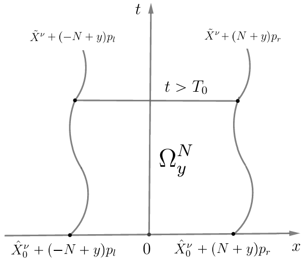
then X~ν\tilde{X}^{\nu} is a Lipschitz continuous curve on [0,+∞).[0,+\infty). For y∈(0,1),N∈ℕ∗y\in(0,1),N\in\mathbb{N}^{*} and t>T0,t>T_{0}, we define the domain

ΩyN\displaystyle\Omega^{N}_{y} :={(x,τ):X~ν(τ)+(−N+y)pl≤x≤X~ν(τ)+(N+y)pr,0≤τ≤t};\displaystyle:=\{(x,\tau):~\tilde{X}^{\nu}(\tau)+(-N+y)p_{l}\leq x\leq\tilde{X}^{\nu}(\tau)+(N+y)p_{r},~0\leq\tau\leq t\};

see Figure 1.

Refer to caption
Figure 1.

It follows from the equations of ulνu_{l}^{\nu} and urνu_{r}^{\nu} that

∬ΩyN{(∂tulν+∂xf⁡(ulν)−ν​∂x2ulν)​gX~νν+(∂turν+∂xf⁡(urν)−ν​∂x2urν)​(1−gX~νν)}​𝑑x​𝑑τ=0.\iint_{\Omega^{N}_{y}}\left\{\left(\partial_{t}u_{l}^{\nu}+\partial_{x}f(u_{l}^{\nu})-\nu\partial_{x}^{2}u_{l}^{\nu}\right)g_{\tilde{X}^{\nu}}^{\nu}+\left(\partial_{t}u_{r}^{\nu}+\partial_{x}f(u_{r}^{\nu})-\nu\partial_{x}^{2}u_{r}^{\nu}\right)(1-g_{\tilde{X}^{\nu}}^{\nu})\right\}dxd\tau=0.

Then integration by parts yields that

(3.9) ∬ΩyN{−(X~ν)′​(t)​(ulν−urν)+(f⁡(ulν)−ν​∂xulν)−(f⁡(urν)−ν​∂xurν)}​(gX~νν)′​𝑑x​𝑑τ\displaystyle\iint_{\Omega^{N}_{y}}\left\{-(\tilde{X}^{\nu})^{\prime}(t)(u_{l}^{\nu}-u_{r}^{\nu})+\left(f(u_{l}^{\nu})-\nu\partial_{x}u_{l}^{\nu}\right)-(f(u_{r}^{\nu})-\nu\partial_{x}u_{r}^{\nu})\right\}(g_{\tilde{X}^{\nu}}^{\nu})^{\prime}dxd\tau
=\displaystyle= AN​(y,t)−AN​(y,0)−BlN​(y,t)+BrN​(y,t),\displaystyle A^{N}(y,t)-A^{N}(y,0)-B_{l}^{N}(y,t)+B_{r}^{N}(y,t),

where

(3.10) AN​(y,t)\displaystyle A^{N}(y,t) :=∫X~ν​(t)+(−N+y)​plX~ν​(t)+(N+y)​pr[ulν​(x,t)​gX~νν​(x)+urν​(x,t)​(1−gX~νν​(x))]​dx,\displaystyle:=\int_{\tilde{X}^{\nu}(t)+(-N+y)p_{l}}^{\tilde{X}^{\nu}(t)+(N+y)p_{r}}\Big[u_{l}^{\nu}(x,t)g_{\tilde{X}^{\nu}}^{\nu}(x)+u_{r}^{\nu}(x,t)(1-g_{\tilde{X}^{\nu}}^{\nu}(x))\Big]dx,
AN​(y,0)\displaystyle A^{N}(y,0) :=∫X^0ν+(−N+y)​plX^0ν+(N+y)​pr[ulν​(x,0)​gX^0νν​(x)+urν​(x,0)​(1−gX^0νν​(x))]​dx,\displaystyle:=\int_{\hat{X}_{0}^{\nu}+(-N+y)p_{l}}^{\hat{X}_{0}^{\nu}+(N+y)p_{r}}\left[u_{l}^{\nu}(x,0)g_{\hat{X}_{0}^{\nu}}^{\nu}(x)+u_{r}^{\nu}(x,0)\left(1-g_{\hat{X}_{0}^{\nu}}^{\nu}(x)\right)\right]dx,
BlN​(y,t)\displaystyle B_{l}^{N}(y,t) :=∫0t{(f(ulν)−ν∂xulν)gX~νν+(f(urν)−ν∂xurν)(1−gX~νν)\displaystyle:=\int_{0}^{t}\Big\{\left(f(u_{l}^{\nu})-\nu\partial_{x}u_{l}^{\nu}\right)g_{\tilde{X}^{\nu}}^{\nu}+\left(f(u_{r}^{\nu})-\nu\partial_{x}u_{r}^{\nu}\right)(1-g_{\tilde{X}^{\nu}}^{\nu})
−(X~ν)′(τ)[ulνgX~νν+urν(1−gX~νν)]}(X~ν(τ)+(−N+y)pl,τ)dτ,\displaystyle-(\tilde{X}^{\nu})^{\prime}(\tau)\left[u_{l}^{\nu}g_{\tilde{X}^{\nu}}^{\nu}+u_{r}^{\nu}(1-g_{\tilde{X}^{\nu}}^{\nu})\right]\Big\}(\tilde{X}^{\nu}(\tau)+(-N+y)p_{l},\tau)d\tau,
BrN​(y,t)\displaystyle B_{r}^{N}(y,t) :=∫0t{(f(ulν)−ν∂xulν)gX~νν+(f(urν)−ν∂xurν)(1−gX~νν)\displaystyle:=\int_{0}^{t}\Big\{\left(f(u_{l}^{\nu})-\nu\partial_{x}u_{l}^{\nu}\right)g_{\tilde{X}^{\nu}}^{\nu}+\left(f(u_{r}^{\nu})-\nu\partial_{x}u_{r}^{\nu}\right)(1-g_{\tilde{X}^{\nu}}^{\nu})
−(X~ν)′(τ)[ulνgX~νν+urν(1−gX~νν)]}(X~ν(τ)+(N+y)pr,τ)dτ.\displaystyle-(\tilde{X}^{\nu})^{\prime}(\tau)\left[u_{l}^{\nu}g_{\tilde{X}^{\nu}}^{\nu}+u_{r}^{\nu}(1-g_{\tilde{X}^{\nu}}^{\nu})\right]\Big\}(\tilde{X}^{\nu}(\tau)+(N+y)p_{r},\tau)d\tau.

It follows from Equation 2.15 and Equation 3.3 that the left hand side of (3.9)

∬ΩyN⋯dxdτ=∬ΩNy∩{0<τ<T0}⋯dxdτ+∬ΩNy∩{T0<τ<t}⋯dxdτ\displaystyle\iint_{\Omega^{N}_{y}}\quad\cdots~dxd\tau=\iint_{\Omega^{N}_{y}\cap\{0<\tau<T_{0}\}}\cdots~dxd\tau\quad+\iint_{\Omega^{N}_{y}\cap\{T_{0}<\tau<t\}}\cdots~dxd\tau
→\displaystyle\rightarrow\quad −M∫0T0(X^ν)′(t)dt+0=−M(X0ν−X^0ν) as N→+∞.\displaystyle-M\int_{0}^{T_{0}}(\hat{X}^{\nu})^{\prime}(t)dt+0=-M(X_{0}^{\nu}-\hat{X}_{0}^{\nu})\qquad\text{ as }N\rightarrow+\infty.

Thus it remains to evaluate the right hand side of (3.9) as N→+∞N\rightarrow+\infty.

(i) The integrals on {τ=0}\{\tau=0\} and {τ=t}\{\tau=t\}.

Set

(3.11) wlν​(x,t):=ulν​(x,t)−u¯l,wrν​(x,t):=urν​(x,t)−u¯r.w_{l}^{\nu}(x,t):=u_{l}^{\nu}(x,t)-\overline{u}_{l},\quad w_{r}^{\nu}(x,t):=u_{r}^{\nu}(x,t)-\overline{u}_{r}.

Then it follows from 2.1 that ‖wlν‖L∞+‖wrν‖L∞≤C​e−α​t.\|w_{l}^{\nu}\|_{L^{\infty}}+\|w_{r}^{\nu}\|_{L^{\infty}}\leq Ce^{-\alpha t}. Since w0​lw_{0l} and w0​rw_{0r} are both of zero average, one has that

(3.12) JN​(y,t)=:AN​(y,t)−AN​(y,0)\displaystyle J^{N}(y,t)=:~A^{N}(y,t)-A^{N}(y,0)
=\displaystyle= ∫(−N+y)​pl(N+y)​pr[wlν​(x+X~ν​(t),t)​gν​(x)+wrν​(x+X~ν​(t),t)​(1−gν​(x))]​𝑑x\displaystyle\int_{(-N+y)p_{l}}^{(N+y)p_{r}}\Big[w_{l}^{\nu}(x+\tilde{X}^{\nu}(t),t)g^{\nu}(x)+w_{r}^{\nu}(x+\tilde{X}^{\nu}(t),t)\left(1-g^{\nu}(x)\right)\Big]dx
−∫X^0ν+(−N+y)​plX^0ν+(N+y)​pr[w0​l(x)gν(x−X^ν0)+w0​r(x)(1−gν(x−X^ν0))]dx\displaystyle-\int_{\hat{X}^{\nu}_{0}+(-N+y)p_{l}}^{\hat{X}^{\nu}_{0}+(N+y)p_{r}}\Big[w_{0l}(x)g^{\nu}(x-\hat{X}^{\nu}_{0})+w_{0r}(x)\left(1-g^{\nu}(x-\hat{X}^{\nu}_{0})\right)\Big]dx
=\displaystyle= O⁡(e−α​t)+∫X^0ν+(−N+y)​plX^0ν+y​pl(w0​l−w0​r)​(x)​(1−gν​(x−X^0ν))​𝑑x\displaystyle O(e^{-\alpha t})+\int_{\hat{X}^{\nu}_{0}+(-N+y)p_{l}}^{\hat{X}^{\nu}_{0}+yp_{l}}(w_{0l}-w_{0r})(x)\left(1-g^{\nu}(x-\hat{X}^{\nu}_{0})\right)dx
−∫X^0ν+y​plX^0ν+y​pr[w0​l(x)gν(x−X^ν0)+w0​r(x)(1−gν(x−X^ν0))]dx\displaystyle-\int_{\hat{X}^{\nu}_{0}+yp_{l}}^{\hat{X}^{\nu}_{0}+yp_{r}}\Big[w_{0l}(x)g^{\nu}(x-\hat{X}^{\nu}_{0})+w_{0r}(x)\left(1-g^{\nu}(x-\hat{X}^{\nu}_{0})\right)\Big]dx
−∫X^0ν+y​prX^0ν+(N+y)​pr(w0​l−w0​r)(x)gν(x−X^ν0)dx.\displaystyle-\int_{\hat{X}^{\nu}_{0}+yp_{r}}^{\hat{X}^{\nu}_{0}+(N+y)p_{r}}(w_{0l}-w_{0r})(x)g^{\nu}(x-\hat{X}^{\nu}_{0})dx.

Then one can get that

(3.13) J⁡(y,t):=\displaystyle J(y,t):= limN→∞JN​(y,t)\displaystyle\lim\limits_{N\rightarrow\infty}J^{N}(y,t)
=\displaystyle= O⁡(e−α​t)+∫−∞X^0ν+y​pl(w0​l−w0​r)​(x)​(1−gν​(x−X^0ν))​𝑑x\displaystyle O(e^{-\alpha t})+\int_{-\infty}^{\hat{X}^{\nu}_{0}+yp_{l}}(w_{0l}-w_{0r})(x)\left(1-g^{\nu}(x-\hat{X}^{\nu}_{0})\right)dx
−∫X^0ν+y​plX^0ν+y​pr[w0​l(x)gν(x−X^ν0)+w0​r(x)(1−gν(x−X^ν0))]dx\displaystyle-\int_{\hat{X}^{\nu}_{0}+yp_{l}}^{\hat{X}^{\nu}_{0}+yp_{r}}\Big[w_{0l}(x)g^{\nu}(x-\hat{X}^{\nu}_{0})+w_{0r}(x)\left(1-g^{\nu}(x-\hat{X}^{\nu}_{0})\right)\Big]dx
−∫X^0ν+y​pr+∞(w0​l−w0​r)(x)gν(x−X^ν0)dx.\displaystyle-\int_{\hat{X}^{\nu}_{0}+yp_{r}}^{+\infty}(w_{0l}-w_{0r})(x)g^{\nu}(x-\hat{X}^{\nu}_{0})dx.

By Equation 3.5, it holds that

(3.14) M⁡(X0νCLOSE\displaystyle M(X_{0}^{\nu} −X^0ν)=−∫ℝ[u0(x)−ϕν(x−X^0ν)−w0​l(x)gν(x−X^0ν)\displaystyle-\hat{X}^{\nu}_{0})=-\int_{\mathbb{R}}\Big[u_{0}(x)-\phi^{\nu}(x-\hat{X}^{\nu}_{0})-w_{0l}(x)g^{\nu}(x-\hat{X}^{\nu}_{0})
−w0​r(x)(1−gν(x−X^0ν))]dx\displaystyle\qquad\qquad\qquad\quad-w_{0r}(x)\left(1-g^{\nu}(x-\hat{X}^{\nu}_{0})\right)\Big]dx
=−∫−∞0(u0−ϕν−w0​l)(x)dx−∫0+∞(u0−ϕν−w0​r)(x)dx\displaystyle=-\int_{-\infty}^{0}\left(u_{0}-\phi^{\nu}-w_{0l}\right)(x)dx-\int_{0}^{+\infty}\left(u_{0}-\phi^{\nu}-w_{0r}\right)(x)dx
+(u¯l−u¯r)​X^0ν−∫−∞0(w0​l−w0​r)​(x)​(1−gν​(x−X^0ν))​𝑑x\displaystyle\quad+(\overline{u}_{l}-\overline{u}_{r})\hat{X}^{\nu}_{0}-\int_{-\infty}^{0}(w_{0l}-w_{0r})(x)\left(1-g^{\nu}(x-\hat{X}^{\nu}_{0})\right)dx
+∫0+∞(w0​l−w0​r)(x)gν(x−X^0ν)dx.\displaystyle\quad+\int_{0}^{+\infty}(w_{0l}-w_{0r})(x)g^{\nu}(x-\hat{X}^{\nu}_{0})dx.

This, together with Equation 3.13, yields that

J⁡(y,t)=\displaystyle J(y,t)=~ O⁡(e−α​t)−M⁡(X0ν−X^0ν)+(u¯l−u¯r)​X^0ν\displaystyle O(e^{-\alpha t})-M(X_{0}^{\nu}-\hat{X}^{\nu}_{0})+(\overline{u}_{l}-\overline{u}_{r})\hat{X}^{\nu}_{0}
−∫−∞0(u0−ϕν−w0​l)(x)dx−∫0+∞(u0−ϕν−w0​r)(x)dx\displaystyle-\int_{-\infty}^{0}\left(u_{0}-\phi^{\nu}-w_{0l}\right)(x)dx-\int_{0}^{+\infty}\left(u_{0}-\phi^{\nu}-w_{0r}\right)(x)dx
+∫0X^0ν+y​plw0​l(x)dx−∫0X^0ν+y​prw0​r(x)dx.\displaystyle+\int_{0}^{\hat{X}^{\nu}_{0}+yp_{l}}w_{0l}(x)dx-\int_{0}^{\hat{X}^{\nu}_{0}+yp_{r}}w_{0r}(x)dx.

Note that for i=l,r,i=l,r, since w0​iw_{0i} has zero average, ∫0yw0​i​(x)​𝑑x\int_{0}^{y}w_{0i}(x)dx is periodic with respective to yy with period pip_{i}. Therefore,

∫01∫0X^0ν+y​piw0​i​(x)​𝑑x​𝑑y\displaystyle\int_{0}^{1}\int_{0}^{\hat{X}^{\nu}_{0}+yp_{i}}w_{0i}(x)dxdy =1pi​∫0pi∫0X^0ν+yw0​i​(x)​𝑑x​𝑑y\displaystyle=\frac{1}{p_{i}}\int_{0}^{p_{i}}\int_{0}^{\hat{X}^{\nu}_{0}+y}w_{0i}(x)dxdy
=1pi​∫0pi∫0yw0​i​(x)​𝑑x​𝑑y.\displaystyle=\frac{1}{p_{i}}\int_{0}^{p_{i}}\int_{0}^{y}w_{0i}(x)dxdy.

Thus one can get that

(3.15) ∫01J⁡(y,t)​𝑑y=\displaystyle\int_{0}^{1}J(y,t)dy=~ O⁡(e−α​t)−M⁡(X0ν−X^0ν)+(u¯l−u¯r)​X^0ν\displaystyle O(e^{-\alpha t})-M(X_{0}^{\nu}-\hat{X}^{\nu}_{0})+(\overline{u}_{l}-\overline{u}_{r})\hat{X}^{\nu}_{0}
−∫−∞0(u0−ϕν−w0​l)(x)dx−∫0+∞(u0−ϕν−w0​r)(x)dx\displaystyle-\int_{-\infty}^{0}\left(u_{0}-\phi^{\nu}-w_{0l}\right)(x)dx-\int_{0}^{+\infty}\left(u_{0}-\phi^{\nu}-w_{0r}\right)(x)dx
+1pl∫0pl∫0yw0​l(x)dxdy−1pr∫0pr∫0yw0​r(x)dxdy.\displaystyle+\frac{1}{p_{l}}\int_{0}^{p_{l}}\int_{0}^{y}w_{0l}(x)dxdy-\frac{1}{p_{r}}\int_{0}^{p_{r}}\int_{0}^{y}w_{0r}(x)dxdy.

(ii) The integrals on two sides.

Since ulνu_{l}^{\nu} is periodic, it holds that

(3.16) BlN​(y,t)=\displaystyle B_{l}^{N}(y,t)= ∫0t{(f(ulν)−ν∂xulν)(X~ν(τ)+ypl,τ)gν((−N+y)pl)\displaystyle\int_{0}^{t}\Big\{\left(f(u_{l}^{\nu})-\nu\partial_{x}u_{l}^{\nu}\right)(\tilde{X}^{\nu}(\tau)+yp_{l},\tau)~g^{\nu}\left((-N+y)p_{l}\right)
−(X~ν)′​(τ)​ulν​(X~ν​(τ)+y​pl,τ)\displaystyle-(\tilde{X}^{\nu})^{\prime}(\tau)~u_{l}^{\nu}(\tilde{X}^{\nu}(\tau)+yp_{l},\tau)
+[⋯](1−gX~νν)(X~ν(τ)+(−N+y)pl,τ)}dτ,\displaystyle+\left[\cdots\right](1-g_{\tilde{X}^{\nu}}^{\nu})(\tilde{X}^{\nu}(\tau)+(-N+y)p_{l},\tau)\Big\}d\tau,

where [⋯][\cdots] denotes the remaining terms which are bounded. Then taking the limit N→+∞N\rightarrow+\infty in Equation 3.16 and using 2.4, one can get that

limN→+∞∫01BlN​(y,t)​𝑑y\displaystyle\lim\limits_{N\rightarrow+\infty}\int_{0}^{1}B_{l}^{N}(y,t)dy =∫0t1pl​∫0plf⁡(ulν)​(X~ν+x,τ)​𝑑x​𝑑τ−∫0t(X~ν)′​(τ)​u¯l​𝑑τ\displaystyle=\int_{0}^{t}\frac{1}{p_{l}}\int_{0}^{p_{l}}f(u_{l}^{\nu})(\tilde{X}^{\nu}+x,\tau)dxd\tau-\int_{0}^{t}(\tilde{X}^{\nu})^{\prime}(\tau)\overline{u}_{l}d\tau
=∫0t1pl​∫0plf⁡(ulν)​(x,τ)​𝑑x​𝑑τ−u¯l​(X~ν​(t)−X^0ν).\displaystyle=\int_{0}^{t}\frac{1}{p_{l}}\int_{0}^{p_{l}}f(u_{l}^{\nu})(x,\tau)dxd\tau-\overline{u}_{l}(\tilde{X}^{\nu}(t)-\hat{X}_{0}^{\nu}).

Similarly, it holds that

limN→+∞∫01BrN​(y,t)​𝑑y=∫0t1pr​∫0prf⁡(urν)​(x,τ)​𝑑x​𝑑τ−u¯r​(X~ν​(t)−X^0ν).\displaystyle\lim\limits_{N\rightarrow+\infty}\int_{0}^{1}B_{r}^{N}(y,t)dy=\int_{0}^{t}\frac{1}{p_{r}}\int_{0}^{p_{r}}f(u_{r}^{\nu})(x,\tau)dxd\tau-\overline{u}_{r}(\tilde{X}^{\nu}(t)-\hat{X}_{0}^{\nu}).

Now, with the calculations in (i) and (ii), one can integrate the equation (3.9) with respect to yy over (0,1),(0,1), and then let N→+∞,N\rightarrow+\infty, to get that for any t>T0,t>T_{0},

(3.17) ∫01J⁡(y,t)​dy+(u¯l−u¯r)​(X~ν​(t)−X^0ν)\displaystyle\int_{0}^{1}J(y,t)dy+(\overline{u}_{l}-\overline{u}_{r})(\tilde{X}^{\nu}(t)-\hat{X}_{0}^{\nu})
=\displaystyle= ∫0t[1pl​∫0plf⁡(ulν)​(x,τ)​dx−1pr​∫0prf⁡(urν)​(x,τ)​dx]​dτ−M⁡(X0ν−X^0ν).\displaystyle\int_{0}^{t}\Big[\frac{1}{p_{l}}\int_{0}^{p_{l}}f(u_{l}^{\nu})(x,\tau)dx-\frac{1}{p_{r}}\int_{0}^{p_{r}}f(u_{r}^{\nu})(x,\tau)dx\Big]d\tau-M(X_{0}^{\nu}-\hat{X}^{\nu}_{0}).

Note also that for i=l,r,i=l,r,

∫0t1pi​∫0pif⁡(uiν)​𝑑y​𝑑τ=\displaystyle\int_{0}^{t}\frac{1}{p_{i}}\int_{0}^{p_{i}}f(u_{i}^{\nu})dyd\tau= ∫0t1pi​∫0pi(f⁡(uiν)−f⁡(u¯i))​𝑑y​𝑑τ+f⁡(u¯i)​t\displaystyle\int_{0}^{t}\frac{1}{p_{i}}\int_{0}^{p_{i}}\left(f(u_{i}^{\nu})-f(\overline{u}_{i})\right)dyd\tau+f(\overline{u}_{i})t
=∫0+∞1pi​∫0pi(f⁡(uiν)−f⁡(u¯i))​𝑑y​𝑑τ+O⁡(e−α​t)+f⁡(u¯i)​t,\displaystyle=\int_{0}^{+\infty}\frac{1}{p_{i}}\int_{0}^{p_{i}}\left(f(u_{i}^{\nu})-f(\overline{u}_{i})\right)dyd\tau+O(e^{-\alpha t})+f(\overline{u}_{i})t,

where 2.1 is used. Then it can follow from Equation 3.15 and Equation 3.17 that for t>T0,t>T_{0},

(3.18) Xν​(t)−s​t=X~ν​(t)−s​t=O⁡(e−α​t)+X∞ν,X^{\nu}(t)-st=\tilde{X}^{\nu}(t)-st=O(e^{-\alpha t})+X_{\infty}^{\nu},

where X∞νX_{\infty}^{\nu} is defined in 1.1. The proof of 2.5 is finished.

3.2. Decay to ansatz

In this section, we will prove 2.7. First, uν​(x,t)u^{\nu}(x,t) will be proved to be close to ulν​(x,t)u^{\nu}_{l}(x,t) (resp., urν​(x,t)u^{\nu}_{r}(x,t)) in the region x<s​t−Nεx<st-N_{\varepsilon} (resp. x>s​t−Nεx>st-N_{\varepsilon}) with large enough tt and NεN_{\varepsilon} (independent of time); see 3.4. Then motivated by [16], the equation of the anti-derivative variable of uν−ψXννu^{\nu}-\psi_{X^{\nu}}^{\nu} is studied and the comparison principle is applied to prove 2.7.

3.2.1. Time-independent estimates

The following result follows directly from 2.3.

Lemma 3.2.

Under the assumptions of 1.1, there holds that

|uν​(x,t)−ψξν​(x,t)|≤C⁡(t)​eβ​|ξ|​e−β​|x−ξ|,ξ,x∈ℝ,t≥0,\displaystyle|u^{\nu}(x,t)-\psi_{\xi}^{\nu}(x,t)|\leq C(t)e^{\beta|\xi|}e^{-\beta|x-\xi|},\qquad\xi,x\in\mathbb{R},t\geq 0,

where C⁡(t)>0C(t)>0 is bounded on any compact subset of [0,+∞).[0,+\infty).

Then by Lemmas 2.3 and 3.2, for any x∈ℝ,t≥0,x\in\mathbb{R},t\geq 0, one can define the anti-derivative variables:

(3.19) Ulν​(x,t)\displaystyle U_{l}^{\nu}(x,t) :=∫−∞x(uν−ulν)​(y,t)​𝑑y,\displaystyle:=\int_{-\infty}^{x}(u^{\nu}-u_{l}^{\nu})(y,t)dy,
(3.20) Urν​(x,t)\displaystyle U_{r}^{\nu}(x,t) :=∫x+∞(uν−urν)​(y,t)​𝑑y,\displaystyle:=\int_{x}^{+\infty}(u^{\nu}-u_{r}^{\nu})(y,t)dy,
(3.21) Uˇξν​(x,t)\displaystyle\check{U}_{\xi}^{\nu}(x,t) :=∫−∞x(uν−ψξν)​(y,t)​𝑑y,\displaystyle:=\int_{-\infty}^{x}(u^{\nu}-\psi_{\xi}^{\nu})(y,t)dy,
(3.22) U^ξν​(x,t)\displaystyle\hat{U}_{\xi}^{\nu}(x,t) :=∫x+∞(uν−ψξν)​(y,t)​𝑑y.\displaystyle:=\int_{x}^{+\infty}(u^{\nu}-\psi_{\xi}^{\nu})(y,t)dy.
Lemma 3.3.

For any C∞C^{\infty} curve ξ(t):[0,+∞)→ℝ\xi(t):[0,+\infty)\rightarrow\mathbb{R} with bounded derivatives, the functions Ulν,Urν,UˇξνU_{l}^{\nu},U_{r}^{\nu},\check{U}_{\xi}^{\nu} and U^ξν\hat{U}_{\xi}^{\nu} defined above satisfy the following equations:

(3.23) ∂tUlν−ν​∂x2Ulν\displaystyle\partial_{t}U_{l}^{\nu}-\nu\partial_{x}^{2}U_{l}^{\nu} =f⁡(ulν)−f⁡(uν),x∈ℝ,t>1,\displaystyle=f(u_{l}^{\nu})-f(u^{\nu}),\qquad x\in\mathbb{R},t>1,
(3.24) ∂tUrν−ν​∂x2Urν\displaystyle\partial_{t}U_{r}^{\nu}-\nu\partial_{x}^{2}U_{r}^{\nu} =f⁡(uν)−f⁡(urν),x∈ℝ,t>1,\displaystyle=f(u^{\nu})-f(u_{r}^{\nu}),\qquad x\in\mathbb{R},t>1,
(3.25) ∂tUˇξν−ν​∂x2Uˇξν\displaystyle\partial_{t}\check{U}_{\xi}^{\nu}-\nu\partial_{x}^{2}\check{U}_{\xi}^{\nu} =f⁡(ψξν)−f⁡(uν)−∫−∞xhξν​(y,t)​𝑑y,x∈ℝ,t>1,\displaystyle=f(\psi_{\xi}^{\nu})-f(u^{\nu})-\int_{-\infty}^{x}h_{\xi}^{\nu}(y,t)dy,\quad x\in\mathbb{R},t>1,
(3.26) ∂tU^ξν−ν​∂x2U^ξν\displaystyle\partial_{t}\hat{U}_{\xi}^{\nu}-\nu\partial_{x}^{2}\hat{U}_{\xi}^{\nu} =f⁡(uν)−f⁡(ψξν)−∫x+∞hξν​(y,t)​𝑑y,x∈ℝ,t>1,\displaystyle=f(u^{\nu})-f(\psi_{\xi}^{\nu})-\int_{x}^{+\infty}h_{\xi}^{\nu}(y,t)dy,\quad x\in\mathbb{R},t>1,

where the derivatives appearing in these equations are all continuous in ℝ×[1,+∞).\mathbb{R}\times[1,+\infty).

Proof.

Here we prove only (3.23) and (3.25), since the proofs of the other two are similar.

  • (1)

    To prove (3.23), for any T>1,T>1, one considers the following problem:

    (3.27) {∂tV−ν∂x2V=f(ulν)−f(uν),x∈ℝ,1<t≤T,V⁡(x,1)=Ulν​(x,1).\begin{cases}&\partial_{t}V-\nu\partial_{x}^{2}V=f(u_{l}^{\nu})-f(u^{\nu}),\quad x\in\mathbb{R},1<t\leq T,\\ &V(x,1)=U_{l}^{\nu}(x,1).\end{cases}

    It follows from 3.2 that

    (3.28) {|f⁡(ulν)−f⁡(uν)|≤C⁡(T)​eβ​x∀x∈ℝ,1<t≤T,|Ulν​(x,1)|≤C​eβ​x∀x∈ℝ.\begin{cases}|f(u_{l}^{\nu})-f(u^{\nu})|\leq C(T)e^{\beta x}&\forall x\in\mathbb{R},1<t\leq T,\\ |U_{l}^{\nu}(x,1)|\leq Ce^{\beta x}&\forall x\in\mathbb{R}.\end{cases}

    Note that

    eβ​|x|≤C⁡(T)​e14​ν​T​|x|2,e^{\beta|x|}\leq C(T)e^{\frac{1}{4\nu T}|x|^{2}},

    and the initial data Ulν​(x,1)U_{l}^{\nu}(x,1) and the source term f⁡(ulν)−f⁡(uν)f(u_{l}^{\nu})-f(u^{\nu}) are smooth functions, then by the standard parabolic theories (see [6, Chapter 1, Theorem 12]), the function

    (3.29) V⁡(x,t)=∫0t−1Kτ​(⋅)∗(f⁡(ulν)−f⁡(uν))​(⋅,t−τ)​𝑑τ+Kt−1​(⋅)∗Ulν​(⋅,1)V(x,t)=\int_{0}^{t-1}K^{\tau}(\cdot)*(f(u_{l}^{\nu})-f(u^{\nu}))(\cdot,t-\tau)d\tau+K^{t-1}(\cdot)*U_{l}^{\nu}(\cdot,1)

    solves (3.27) and all the derivatives of VV appearing in the equation exist and are continuous in ℝ×[1,T],\mathbb{R}\times[1,T], where Kt​(x):=(2​π​ν​t)−12​e−x24​ν​tK^{t}(x):=(2\pi\nu t)^{-\frac{1}{2}}e^{-\frac{x^{2}}{4\nu t}} denotes the heat kernel. It then follows from (3.28) and (3.29) that V⁡(x,t)V(x,t) vanishes as x→−∞.x\rightarrow-\infty. Then by (3.29) and the equations of uνu^{\nu} and ulν,u_{l}^{\nu}, it holds that

    ∂xV⁡(x,t)\displaystyle\partial_{x}V(x,t) =∫0t−1[∂xKτ∗(f⁡(ulν)−f⁡(u))]​(x,t−τ)​𝑑τ\displaystyle=\int_{0}^{t-1}\left[\partial_{x}K^{\tau}*(f(u_{l}^{\nu})-f(u))\right](x,t-\tau)d\tau
    +[Kt−1∗(u−ulν)]​(x,1)\displaystyle+\left[K^{t-1}*(u-u_{l}^{\nu})\right](x,1)
    =(u−ulν)(x,t),x∈ℝ,1≤t≤T,\displaystyle=(u-u_{l}^{\nu})(x,t),\qquad\qquad x\in\mathbb{R},1\leq t\leq T,

    which implies that V⁡(x,t)=Ulν​(x,t)V(x,t)=U_{l}^{\nu}(x,t) for all x∈ℝx\in\mathbb{R} and 1≤t≤T.1\leq t\leq T. And since T>1T>1 is arbitrary, (3.23) holds true.

  • (2)

    Now we prove (3.25). By integrating (2.11) with the space variable on (−∞,x),(-\infty,x), one can get from Lemmas 2.1 and 2.4 that

    ∫−∞xhξν​dy=\displaystyle\int_{-\infty}^{x}h_{\xi}^{\nu}~dy= (f⁡(ψξν)−f⁡(ulν))​gξν+(f⁡(ψξν)−f⁡(urν))​(1−gξν)\displaystyle\left(f(\psi_{\xi}^{\nu})-f(u_{l}^{\nu})\right)g_{\xi}^{\nu}+\left(f(\psi_{\xi}^{\nu})-f(u_{r}^{\nu})\right)(1-g_{\xi}^{\nu})
    −2​ν​(ulν−urν)​(gξν)′+∫−∞x(f⁡(ulν)−f⁡(urν))​(gξν)′​𝑑y\displaystyle-2\nu(u_{l}^{\nu}-u_{r}^{\nu})(g_{\xi}^{\nu})^{\prime}+\int_{-\infty}^{x}(f(u_{l}^{\nu})-f(u_{r}^{\nu}))(g_{\xi}^{\nu})^{\prime}~dy
    −ξ′(t)∫−∞x(ulν−urν)(gξν)′dy+ν∫−∞x(ulν−urν)(gξν)′′dy,\displaystyle-\xi^{\prime}(t)\int_{-\infty}^{x}(u_{l}^{\nu}-u_{r}^{\nu})(g_{\xi}^{\nu})^{\prime}~dy+\nu\int_{-\infty}^{x}(u_{l}^{\nu}-u_{r}^{\nu})(g_{\xi}^{\nu})^{\prime\prime}~dy,

    is smooth. And it follows from Lemmas 2.4, 3.2 and ψξν−ulν=−(ulν−urν)​(1−gξν)\psi_{\xi}^{\nu}-u_{l}^{\nu}=-(u_{l}^{\nu}-u_{r}^{\nu})(1-g_{\xi}^{\nu}) that for any T>1,T>1,

    |∫−∞xhξν​𝑑y|≤C⁡(T)​[1−gξν​(x)+|(gξν)′​(x)|+∫−∞x|(gξν)′|​𝑑y+∫−∞x|(gξν)′′|​𝑑y].\Big|\int_{-\infty}^{x}h_{\xi}^{\nu}~dy\Big|\leq C(T)\Big[1-g_{\xi}^{\nu}(x)+|(g_{\xi}^{\nu})^{\prime}(x)|+\int_{-\infty}^{x}|(g_{\xi}^{\nu})^{\prime}|dy+\int_{-\infty}^{x}|(g_{\xi}^{\nu})^{\prime\prime}|dy\Big].

    Note that ∫−∞x|(gξν)′|​𝑑y=1−gξν.\int_{-\infty}^{x}|(g_{\xi}^{\nu})^{\prime}|dy=1-g_{\xi}^{\nu}. And by (gν)′′=1u¯l−u¯r​(f′​(ϕν)−s)​(ϕν)′,(g^{\nu})^{\prime\prime}=\frac{1}{\overline{u}_{l}-\overline{u}_{r}}(f^{\prime}(\phi^{\nu})-s)(\phi^{\nu})^{\prime}, there exists a unique point x0∈ℝx_{0}\in\mathbb{R} such that (gν)′′<0(g^{\nu})^{\prime\prime}<0 for x<x0,x<x_{0}, and (gν)′′>0(g^{\nu})^{\prime\prime}>0 for x>x0.x>x_{0}. Then ∫−∞x|(gξν)′′|​𝑑y=−(gξν)′\int_{-\infty}^{x}|(g_{\xi}^{\nu})^{\prime\prime}|dy=-(g^{\nu}_{\xi})^{\prime} if x<x0+ξ.x<x_{0}+\xi. Hence, it follows from 2.4 that

    (3.30) |∫−∞xhξν​𝑑y|≤C⁡(T)​eβ​x∀x∈ℝ,1≤t≤T.\Big|\int_{-\infty}^{x}h_{\xi}^{\nu}~dy\Big|\leq C(T)e^{\beta x}\qquad\forall x\in\mathbb{R},1\leq t\leq T.

    By 3.2, one can verify easily that

    (3.31) |Uˇξ⁡(1)ν​(x,1)|≤C​eβ​x∀x∈ℝ.|\check{U}^{\nu}_{\xi(1)}(x,1)|\leq Ce^{\beta x}\qquad\quad\forall x\in\mathbb{R}.

    Now we consider the problem:

    (3.32) {∂tVˇ−ν​∂x2Vˇ=Hˇν:=f⁡(ψξν)−f⁡(uν)−∫−∞xhξν​(y,t)​dy,x∈ℝ,1<t≤T,Vˇ​(x,1)=Uˇξ⁡(1)ν​(x,1),x∈ℝ.\begin{cases}\partial_{t}\check{V}-\nu\partial_{x}^{2}\check{V}=\check{H}^{\nu}:=f(\psi_{\xi}^{\nu})-f(u^{\nu})-\int_{-\infty}^{x}h^{\nu}_{\xi}(y,t)dy,&x\in\mathbb{R},1<t\leq T,\\ \check{V}(x,1)=\check{U}^{\nu}_{\xi(1)}(x,1),&x\in\mathbb{R}.\end{cases}

    By 3.2 and (3.30), Hˇν\check{H}^{\nu} satisfies that

    (3.33) |Hˇν​(x,t)|≤C⁡(T)​eβ​x∀x∈ℝ,1<t≤T.|\check{H}^{\nu}(x,t)|\leq C(T)e^{\beta x}\qquad\forall x\in\mathbb{R},1<t\leq T.

    Then similar to the proof in (1), since the initial data Uˇξ⁡(1)ν​(x,1)\check{U}^{\nu}_{\xi(1)}(x,1) is smooth and satisfies (3.31), and the source term Hˇν\check{H}^{\nu} is smooth and satisfies (3.33), one can obtain that the function

    (3.34) Vˇ​(x,t)=∫0t−1Kτ​(⋅)∗Hˇν​(⋅,t−τ)​𝑑τ+Kt−1​(⋅)∗Uˇξ⁡(1)ν​(⋅,1)\check{V}(x,t)=\int_{0}^{t-1}K^{\tau}(\cdot)*\check{H}^{\nu}(\cdot,t-\tau)d\tau+K^{t-1}(\cdot)*\check{U}^{\nu}_{\xi(1)}(\cdot,1)

    solves (3.32) and all the derivatives of Vˇ\check{V} appearing in the equation exist and are continuous in ℝ×[1,T].\mathbb{R}\times[1,T]. It follows from (3.33) and (3.34) that Vˇ​(x,t)\check{V}(x,t) vanishes as x→−∞.x\rightarrow-\infty. Then (3.34) and the equation of ψξν\psi_{\xi}^{\nu} yield

    ∂t(uν−ψξν)−ν​∂x2(uν−ψξν)\displaystyle\partial_{t}(u^{\nu}-\psi_{\xi}^{\nu})-\nu\partial_{x}^{2}(u^{\nu}-\psi_{\xi}^{\nu}) =∂x[f⁡(ψξν)−f⁡(uν)−∫−∞xhξν​(y,t)​𝑑y]\displaystyle=\partial_{x}[f(\psi_{\xi}^{\nu})-f(u^{\nu})-\int_{-\infty}^{x}h_{\xi}^{\nu}(y,t)dy]
    =∂xHˇν.\displaystyle=\partial_{x}\check{H}^{\nu}.

    And then

    ∂xVˇ​(x,t)\displaystyle\partial_{x}\check{V}(x,t) =∫0t−1∂xKτ​(⋅)∗Hˇν​(⋅,t−τ)​dτ+Kt−1​(⋅)∗(uν−ψξν)​(⋅,1)\displaystyle=\int_{0}^{t-1}\partial_{x}K^{\tau}(\cdot)*\check{H}^{\nu}(\cdot,t-\tau)d\tau+K^{t-1}(\cdot)*(u^{\nu}-\psi_{\xi}^{\nu})(\cdot,1)
    =(uν−ψξν)(x,t)∀x∈ℝ,1<t≤T,\displaystyle=(u^{\nu}-\psi_{\xi}^{\nu})(x,t)\qquad\qquad\forall x\in\mathbb{R},1<t\leq T,

    which implies that Vˇ=Uˇξν.\check{V}=\check{U}_{\xi}^{\nu}.

∎

Now we choose a fixed small number ε0>0\varepsilon_{0}>0 such that

(3.35) f′​(u¯l−2​ε0)−s>0​ and ​f′​(u¯r+2​ε0)−s<0.f^{\prime}(\overline{u}_{l}-2\varepsilon_{0})-s>0~\text{ and }~f^{\prime}(\overline{u}_{r}+2\varepsilon_{0})-s<0.

Then it can follow from 2.1 that there exists T1>T0T_{1}>T_{0} large enough such that

(3.36) ulν​(x,t)>u¯l−ε0​ and ​urν​(x,t)<u¯r+ε0∀x∈ℝ,t>T1,u_{l}^{\nu}(x,t)>\overline{u}_{l}-\varepsilon_{0}~\text{ and }~u_{r}^{\nu}(x,t)<\overline{u}_{r}+\varepsilon_{0}\qquad\forall x\in\mathbb{R},~t>T_{1},

where T0T_{0} is the number chosen in Equation 2.13.

For later use, we define

(3.37) a⁡(v,w)\displaystyle a(v,w) :=∫01f′​(w+ρ⁡(v−w))​𝑑ρ,\displaystyle:=\int_{0}^{1}f^{\prime}(w+\rho(v-w))\ d\rho,
(3.38) b⁡(v,w)\displaystyle b(v,w) :=∫01f′′​(w+ρ⁡(v−w))​𝑑ρ.\displaystyle:=\int_{0}^{1}f^{\prime\prime}(w+\rho(v-w))\ d\rho.

Now, we give the results of the time-independent estimates of uν−ulνu^{\nu}-u_{l}^{\nu} and uν−urν.u^{\nu}-u_{r}^{\nu}.

Proposition 3.4.

Under the assumptions of 1.1. There exists T2>T1T_{2}>T_{1} such that for any ε>0\varepsilon>0, there exists N⁡(ε)>0,N(\varepsilon)>0, independent of time t,t, such that

(3.39) |uν​(x,t)−ulν​(x,t)|≤ε,t>T2,x<s​t−N⁡(ε),\displaystyle|u^{\nu}(x,t)-u_{l}^{\nu}(x,t)|\leq\varepsilon,\qquad t>T_{2},x<st-N(\varepsilon),
(3.40) |uν​(x,t)−urν​(x,t)|≤ε,t>T2,x>s​t+N⁡(ε).\displaystyle|u^{\nu}(x,t)-u_{r}^{\nu}(x,t)|\leq\varepsilon,\qquad t>T_{2},x>st+N(\varepsilon).
Proof.

We prove (3.39) only, since the proof of (3.40) is similar. And the proof will be divided into four steps.

S​t​e​p​1.Step~1. We will prove that there exist T2>T1,T_{2}>T_{1}, independent of ε,\varepsilon, and N1=N1​(ε)>0N_{1}=N_{1}(\varepsilon)>0 such that

Ulν​(x,t)<ε,t>T2,x<s​t−N1,U_{l}^{\nu}(x,t)<\varepsilon,\quad t>T_{2},~x<st-N_{1},

where UlνU_{l}^{\nu} is defined in (3.19).

By (3.35), one can define a constant

(3.41) β~:=f′​(u¯l−2​ε0)−s>0.\tilde{\beta}:=f^{\prime}(\overline{u}_{l}-2\varepsilon_{0})-s>0.

For a constant M1>1M_{1}>1 to be determined later (see Equation 3.47), we define the function:

(3.42) u~​(x,t):=M1​eβ~​(x−s​t)+ulν​(x,t),x∈ℝ,t>0.\tilde{u}(x,t):=M_{1}e^{\tilde{\beta}(x-st)}+u_{l}^{\nu}(x,t),\quad x\in\mathbb{R},t>0.

Then by the equation of ulν,u_{l}^{\nu}, one has that

(3.43) ∂tu~−ν​∂x2u~+∂xf⁡(u~)=h~:=−β~​s​M1​eβ~​(x−s​t)−ν​β~2​M1​eβ~​(x−s​t)+∂x(f⁡(u~)−f⁡(ulν)).\partial_{t}\tilde{u}-\nu\partial_{x}^{2}\tilde{u}+\partial_{x}f(\tilde{u})=\tilde{h}:=-\tilde{\beta}sM_{1}e^{\tilde{\beta}(x-st)}-\nu\tilde{\beta}^{2}M_{1}e^{\tilde{\beta}(x-st)}+\partial_{x}\left(f(\tilde{u})-f(u_{l}^{\nu})\right).

Since ff is strictly convex, (3.36) implies that

f′​(u~)≥f′​(ulν)≥f′​(u¯l−ε0)∀x∈ℝ,t≥T1.f^{\prime}(\tilde{u})\geq f^{\prime}(u_{l}^{\nu})\geq f^{\prime}(\overline{u}_{l}-\varepsilon_{0})\quad\forall x\in\mathbb{R},t\geq T_{1}.

Hence, for the given constant M1,M_{1}, if t≥T1,t\geq T_{1}, the following two inequalities hold.

  1. (1)

    If xx satisfies M​eβ~​(x−s​t)≥1Me^{\tilde{\beta}(x-st)}\geq 1, then it holds that

    ∂x(f⁡(u~)−f⁡(ulν))\displaystyle\partial_{x}\left(f(\tilde{u})-f(u_{l}^{\nu})\right) =(f′​(u~)−f′​(ulν))​(β~​M1​eβ~​(x−s​t)+∂xulν)+f′​(ulν)​β~​M1​eβ~​(x−s​t)\displaystyle=\left(f^{\prime}(\tilde{u})-f^{\prime}(u_{l}^{\nu})\right)\left(\tilde{\beta}M_{1}e^{\tilde{\beta}(x-st)}+\partial_{x}u_{l}^{\nu}\right)+f^{\prime}(u_{l}^{\nu})\tilde{\beta}M_{1}e^{\tilde{\beta}(x-st)}
    ≥(f′​(u~)−f′​(ulν))​(β~−|∂xulν|)+f′​(u¯l−ε0)​β~​M1​eβ~​(x−s​t).\displaystyle\geq\left(f^{\prime}(\tilde{u})-f^{\prime}(u_{l}^{\nu})\right)\left(\tilde{\beta}-|\partial_{x}u_{l}^{\nu}|\right)+f^{\prime}(\overline{u}_{l}-\varepsilon_{0})\tilde{\beta}M_{1}e^{\tilde{\beta}(x-st)}.

    Then by Equation 3.43, 2.4 and ν≤1,\nu\leq 1, one has that

    h~≥\displaystyle\tilde{h}\geq (f′​(u~)−f′​(ulν))​(β~−|∂xulν|)+β~​M1​eβ~​(x−s​t)​(f′​(u¯l−ε0)−(s+β~))\displaystyle\left(f^{\prime}(\tilde{u})-f^{\prime}(u_{l}^{\nu})\right)\left(\tilde{\beta}-|\partial_{x}u_{l}^{\nu}|\right)+\tilde{\beta}M_{1}e^{\tilde{\beta}(x-st)}\left(f^{\prime}(\overline{u}_{l}-\varepsilon_{0})-(s+\tilde{\beta})\right)
    ≥\displaystyle\geq (f′​(u~)−f′​(ulν))​(β~−C​e−α​t)+β~​M1​eβ~​(x−s​t)​(f′​(u¯l−ε0)−f′​(u¯l−2​ε0))\displaystyle\left(f^{\prime}(\tilde{u})-f^{\prime}(u_{l}^{\nu})\right)\left(\tilde{\beta}-Ce^{-\alpha t}\right)+\tilde{\beta}M_{1}e^{\tilde{\beta}(x-st)}\left(f^{\prime}(\overline{u}_{l}-\varepsilon_{0})-f^{\prime}(\overline{u}_{l}-2\varepsilon_{0})\right)
    ≥\displaystyle\geq (f′​(u~)−f′​(ulν))​(β~−C​e−α​t).\displaystyle\left(f^{\prime}(\tilde{u})-f^{\prime}(u_{l}^{\nu})\right)\left(\tilde{\beta}-Ce^{-\alpha t}\right).
  2. (2)

    If xx satisfies M1​eβ~​(x−s​t)<1M_{1}e^{\tilde{\beta}(x-st)}<1, one has 0<u~−ulν≤10<\tilde{u}-u_{l}^{\nu}\leq 1. Then it holds that

    ∂x(f⁡(u~)−f⁡(ulν))\displaystyle\partial_{x}\left(f(\tilde{u})-f(u_{l}^{\nu})\right) =f′​(u~)​β~​M​eβ~​(x−s​t)+(f′​(u~)−f′​(ulν))​∂xulν\displaystyle=f^{\prime}(\tilde{u})\tilde{\beta}Me^{\tilde{\beta}(x-st)}+\left(f^{\prime}(\tilde{u})-f^{\prime}(u_{l}^{\nu})\right)\partial_{x}u_{l}^{\nu}
    =f′​(u~)​β~​M1​eβ~​(x−s​t)+f′′​(⋅)​(u~−ulν)​∂xulν\displaystyle=f^{\prime}(\tilde{u})\tilde{\beta}M_{1}e^{\tilde{\beta}(x-st)}+f^{\prime\prime}(\cdot)(\tilde{u}-u_{l}^{\nu})\partial_{x}u_{l}^{\nu}
    ≥f′​(u¯l−ε0)​β~​M1​eβ~​(x−s​t)−C​M1​eβ~​(x−s​t)​|∂xulν|.\displaystyle\geq f^{\prime}(\overline{u}_{l}-\varepsilon_{0})\tilde{\beta}M_{1}e^{\tilde{\beta}(x-st)}-CM_{1}e^{\tilde{\beta}(x-st)}|\partial_{x}u_{l}^{\nu}|.

    This yields that

    h~≥\displaystyle\tilde{h}\geq β~​M1​eβ~​(x−s​t)​(f′​(u¯l−ε0)−(s+β~))−C​M1​eβ~​(x−s​t)​|∂xulν|\displaystyle~\tilde{\beta}M_{1}e^{\tilde{\beta}(x-st)}\left(f^{\prime}(\overline{u}_{l}-\varepsilon_{0})-(s+\tilde{\beta})\right)-CM_{1}e^{\tilde{\beta}(x-st)}|\partial_{x}u_{l}^{\nu}|
    ≥\displaystyle\geq M1​eβ~​(x−s​t)​[β~​(f′​(u¯l−ε0)−(s+β~))−C​e−α​t]\displaystyle~M_{1}e^{\tilde{\beta}(x-st)}\left[\tilde{\beta}\left(f^{\prime}(\overline{u}_{l}-\varepsilon_{0})-(s+\tilde{\beta})\right)-Ce^{-\alpha t}\right]
    ≥\displaystyle\geq M1​eβ~​(x−s​t)​[β~​(f′​(u¯l−ε0)−f′​(u¯l−2​ε0))−C​e−α​t]\displaystyle~M_{1}e^{\tilde{\beta}(x-st)}\left[\tilde{\beta}\left(f^{\prime}(\overline{u}_{l}-\varepsilon_{0})-f^{\prime}(\overline{u}_{l}-2\varepsilon_{0})\right)-Ce^{-\alpha t}\right]
    ≥\displaystyle\geq M1​eβ~​(x−s​t)​(β~​c0​ε0−C​e−α​t),\displaystyle~M_{1}e^{\tilde{\beta}(x-st)}\left(\tilde{\beta}c_{0}\varepsilon_{0}-Ce^{-\alpha t}\right),

    where c0:=min⁡f′′>0.c_{0}:=\min f^{\prime\prime}>0.

As a result of (1) and (2), there exists a constant T2>T1,T_{2}>T_{1}, independent of either M1M_{1} or ε,\varepsilon, such that

h~=∂tu~−ν​∂x2u~+∂xf⁡(u~)>0,x∈ℝ,t≥T2.\tilde{h}=\partial_{t}\tilde{u}-\nu\partial_{x}^{2}\tilde{u}+\partial_{x}f(\tilde{u})>0,\qquad x\in\mathbb{R},t\geq T_{2}.

Set U~​(x,t):=∫−∞x(uν−u~)​(y,t)​𝑑y.\tilde{U}(x,t):=\int_{-\infty}^{x}(u^{\nu}-\tilde{u})(y,t)dy. Then as for the proof of Lemma 3.3, one can prove that

∂tU~−ν∂x2U~+(f(uν)−f(u~))=−∫−∞xh~(y,t)dy,x∈ℝ,t>T2,\partial_{t}\tilde{U}-\nu\partial_{x}^{2}\tilde{U}+\left(f(u^{\nu})-f(\tilde{u})\right)=-\int_{-\infty}^{x}\tilde{h}(y,t)dy,\qquad x\in\mathbb{R},t>T_{2},

which implies that

(3.44) ∂tU~−ν​∂x2U~+a⁡(uν,u~)​∂xU~<0∀x∈ℝ,t>T2,\partial_{t}\tilde{U}-\nu\partial_{x}^{2}\tilde{U}+a(u^{\nu},\tilde{u})\partial_{x}\tilde{U}<0\qquad\forall x\in\mathbb{R},t>T_{2},

where a⁡(u,v)a(u,v) is defined by (3.37).

By 3.2, there exists N1>0N_{1}>0 such that

(3.45) |Ulν​(x,T2)|=|∫−∞x(uν−ulν)​(y,T2)​𝑑y|≤ε∀x≤−N1.|U_{l}^{\nu}(x,T_{2})|=\Big|\int_{-\infty}^{x}(u^{\nu}-u_{l}^{\nu})(y,T_{2})dy\Big|\leq\varepsilon\quad\forall x\leq-N_{1}.

For this N1,N_{1}, it can also follow from 3.2 that one can define a constant

(3.46) B:=supx≥−N1|∫−N1x(uν−urν)​(y,T2)​𝑑y|<+∞.B:=\sup_{x\geq-N_{1}}\Big|\int_{-N_{1}}^{x}(u^{\nu}-u_{r}^{\nu})(y,T_{2})dy\Big|<+\infty.

Thus, for the given constants β~,T2,N1\tilde{\beta},T_{2},N_{1} and B,B, one can choose M1>0M_{1}>0 large enough such that

(3.47) ∫−∞−N1(ulν−u~)​(y,T2)​𝑑y=−M1β~​e−β~​(N1+s​T2)<−B.\int_{-\infty}^{-N_{1}}(u_{l}^{\nu}-\tilde{u})(y,T_{2})dy=-\frac{M_{1}}{\tilde{\beta}}e^{-\tilde{\beta}(N_{1}+sT_{2})}<-B.

Now we claim that

C​l​a​i​m​1.Claim~1.

U~​(x,T2)=∫−∞x(uν−u~)​(y,T2)​𝑑y≤ε∀x∈ℝ.\tilde{U}(x,T_{2})=\int_{-\infty}^{x}(u^{\nu}-\tilde{u})(y,T_{2})dy\leq\varepsilon\quad\forall x\in\mathbb{R}.

In fact, if x≤−N1,x\leq-N_{1}, then (3.45) implies that

∫−∞x(uν−u~)​(y,T2)​𝑑y≤∫−∞x(uν−ulν)​(y,T2)​𝑑y≤ε.\int_{-\infty}^{x}(u^{\nu}-\tilde{u})(y,T_{2})dy\leq\int_{-\infty}^{x}(u^{\nu}-u_{l}^{\nu})(y,T_{2})dy\leq\varepsilon.

And if x>−N1,x>-N_{1}, it follows from (3.45) and (3.46) that

∫−∞x(uν−u~)​(y,T2)​𝑑y=\displaystyle\int_{-\infty}^{x}(u^{\nu}-\tilde{u})(y,T_{2})dy= ∫−∞−N1(uν−ulν)+∫−∞−N1(ulν−u~)\displaystyle\int_{-\infty}^{-N_{1}}(u^{\nu}-u_{l}^{\nu})+\int_{-\infty}^{-N_{1}}(u_{l}^{\nu}-\tilde{u})
+∫−N1x(uν−urν)+∫−N1x(urν−u~)\displaystyle+\int_{-N_{1}}^{x}(u^{\nu}-u_{r}^{\nu})+\int_{-N_{1}}^{x}(u_{r}^{\nu}-\tilde{u})
≤\displaystyle\leq ε−B+B+0=ε,\displaystyle~\varepsilon-B+B+0=\varepsilon,

which proves C​l​a​i​m​1.Claim~1.

Combing (3.44) with C​l​a​i​m​1Claim~1, and using the maximum principle [16, Lemma 1], one can obtain that

U~​(x,t)≤ε∀x∈ℝ,t≥T2,\tilde{U}(x,t)\leq\varepsilon\qquad\forall x\in\mathbb{R},t\geq T_{2},

which implies that

Ulν​(x,t)=∫−∞x(uν−ulν)​(y,t)​𝑑y=U~​(x,t)+M1β~​eβ~​(x−s​t)≤2​ε,U_{l}^{\nu}(x,t)=\int_{-\infty}^{x}(u^{\nu}-u_{l}^{\nu})(y,t)dy=\tilde{U}(x,t)+\frac{M_{1}}{\tilde{\beta}}e^{\tilde{\beta}(x-st)}\leq 2\varepsilon,

if t≥T2t\geq T_{2} and x−s​t<−N1x-st<-N_{1} with N1>0N_{1}>0 large enough.

S​t​e​p​2.Step~2. In this step, it is aimed to construct a “sub-solution” ψξν\psi_{\xi}^{\nu} to Equation 1.1 such that the anti-derivative variable of uν−ψξνu^{\nu}-\psi_{\xi}^{\nu} has the lower bound −ε-\varepsilon (see Equation 3.55). The idea is to find a C∞C^{\infty} curve ξ(t):[T2,+∞)→ℝ\xi(t):[T_{2},+\infty)\rightarrow\mathbb{R} such that the ansatz ψξν\psi_{\xi}^{\nu} defined by (2.8) satisfies that

(3.48) hξν=∂tψξν+∂xf⁡(ψξν)−ν​∂x2ψξν<0∀x∈ℝ,t>T2,h_{\xi}^{\nu}=\partial_{t}\psi_{\xi}^{\nu}+\partial_{x}f(\psi_{\xi}^{\nu})-\nu\partial_{x}^{2}\psi_{\xi}^{\nu}<0\qquad\forall x\in\mathbb{R},t>T_{2},

with the proper initial data Equation 3.53.

For two given constants M2>0M_{2}>0 and d>0d>0, where M2M_{2} will be determined in this step, and dd will be determined in the next step, we define a C∞C^{\infty} curves ξ(t):[T2,+∞)→ℝ,\xi(t):[T_{2},+\infty)\rightarrow\mathbb{R}, which solves the following problem:

(3.49) {ξ′(t)=s−M2e−α​t,t>T2,ξ⁡(T2)=−d.\begin{cases}&\xi^{\prime}(t)=s-M_{2}e^{-\alpha t},\qquad t>T_{2},\\ &\xi(T_{2})=-d.\end{cases}

Then by (3.49), there exists a constant D>d,D>d, depending on α,T2,d\alpha,T_{2},d and M2,M_{2}, such that

(3.50) ξ⁡(t)∈[s​t−D,s​t+D]∀t≥T2.\xi(t)\in[st-D,st+D]\quad\forall~t\geq T_{2}.

Now we calculate the source term hξν.h_{\xi}^{\nu}. It follows from (2.12) and (2.13) that for t≥T2,t\geq T_{2},

hξν=\displaystyle h_{\xi}^{\nu}= (ulν−urν)​(ξ′​(t)−s+f′​(ϕξν)−f′​(ψξν)+2​ν​∂xulν−∂xurνulν−urν)​|(gξν)′|\displaystyle~(u_{l}^{\nu}-u_{r}^{\nu})\left(\xi^{\prime}(t)-s+f^{\prime}(\phi_{\xi}^{\nu})-f^{\prime}(\psi_{\xi}^{\nu})+2\nu\dfrac{\partial_{x}u_{l}^{\nu}-\partial_{x}u_{r}^{\nu}}{u_{l}^{\nu}-u_{r}^{\nu}}\right)\lvert(g_{\xi}^{\nu})^{\prime}\rvert
−(ulν−urν)​(b⁡(ψξν,ulν)​∂xulν−b⁡(ψξν,urν)​∂xurν)​gξν​(1−gξν),\displaystyle-(u_{l}^{\nu}-u_{r}^{\nu})\left(b(\psi_{\xi}^{\nu},u_{l}^{\nu})\partial_{x}u_{l}^{\nu}-b(\psi_{\xi}^{\nu},u_{r}^{\nu})\partial_{x}u_{r}^{\nu}\right)g_{\xi}^{\nu}(1-g_{\xi}^{\nu}),

where b⁡(u,v)b(u,v) is defined in (3.38). Then by 2.1 and (2.4), one has that for t≥T2,t\geq T_{2},

hξν≤\displaystyle h_{\xi}^{\nu}\leq (ulν−urν)​(ξ′​(t)−s+f′​(ϕξν)−f′​(ψξν)+2​ν​∂xulν−∂xurνulν−urν)​|(gξν)′|\displaystyle~(u_{l}^{\nu}-u_{r}^{\nu})\left(\xi^{\prime}(t)-s+f^{\prime}(\phi_{\xi}^{\nu})-f^{\prime}(\psi_{\xi}^{\nu})+2\nu\dfrac{\partial_{x}u_{l}^{\nu}-\partial_{x}u_{r}^{\nu}}{u_{l}^{\nu}-u_{r}^{\nu}}\right)\lvert(g_{\xi}^{\nu})^{\prime}\rvert
+C⁡(ulν−urν)​(|∂xurν|+|∂xulν|)​|(gξν)′|\displaystyle+C(u_{l}^{\nu}-u_{r}^{\nu})\left(\lvert\partial_{x}u_{r}^{\nu}\rvert+\lvert\partial_{x}u_{l}^{\nu}\rvert\right)\lvert(g_{\xi}^{\nu})^{\prime}\rvert
≤\displaystyle\leq (ulν−urν)​|(gξν)′|​[−M2​e−α​t+C​|ϕξν−ψξν|+C⁡(|∂xurν|+|∂xulν|)].\displaystyle~(u_{l}^{\nu}-u_{r}^{\nu})~\lvert(g_{\xi}^{\nu})^{\prime}\rvert~\Big[-M_{2}e^{-\alpha t}+C\lvert\phi_{\xi}^{\nu}-\psi_{\xi}^{\nu}\rvert+C(\lvert\partial_{x}u_{r}^{\nu}\rvert+\lvert\partial_{x}u_{l}^{\nu}\rvert)\Big].

Note that

|ϕξν−ψξν|≤|u¯l−ulν|gξν+|u¯r−urν|(1−gξν)≤C​e−α​t∀x∈ℝ.|\phi_{\xi}^{\nu}-\psi_{\xi}^{\nu}|\leq|\overline{u}_{l}-u_{l}^{\nu}|g_{\xi}^{\nu}+|\overline{u}_{r}-u_{r}^{\nu}|(1-g_{\xi}^{\nu})\leq Ce^{-\alpha t}\qquad\forall x\in\mathbb{R}.

Then if M>0M>0 is large enough, it holds that

hξν≤(ulν−urν)​|(gξν)′|​(−M2+C)​e−α​t<0∀x∈ℝ,t>T2.\displaystyle h_{\xi}^{\nu}\leq(u_{l}^{\nu}-u_{r}^{\nu})~\lvert(g_{\xi}^{\nu})^{\prime}\rvert~(-M_{2}+C)e^{-\alpha t}<0\qquad\forall x\in\mathbb{R},t>T_{2}.

Therefore, for M2>0M_{2}>0 large enough, (3.48) is fulfilled with the ξ\xi constructed in (3.49).

S​t​e​p​3.Step~3. In this step, we will prove that there exists N2=N2​(ε)>0N_{2}=N_{2}(\varepsilon)>0 such that

(3.51) Ulν​(x,t)>−ε,t>T2,x<s​t−N2.U_{l}^{\nu}(x,t)>-\varepsilon,\quad t>T_{2},~x<st-N_{2}.

For the constants N1N_{1} and BB defined in (3.45) and (3.46), one can choose the constant d=ξ⁡(T2)>0d=\xi(T_{2})>0 (which is in (3.49)) large enough such that

(3.52) ∫−∞−N1(ulν−ψ−dν)​(x,T2)​𝑑x+∫−N1+∞(urν−ψ−dν)​(x,T2)​𝑑x\displaystyle\int_{-\infty}^{-N_{1}}(u_{l}^{\nu}-\psi_{-d}^{\nu})(x,T_{2})dx+\int_{-N_{1}}^{+\infty}(u_{r}^{\nu}-\psi_{-d}^{\nu})(x,T_{2})dx
=\displaystyle= ∫−∞−N1(ulν−urν)​(x,T2)​(1−gν​(x+d))​𝑑x−∫−N1+∞(ulν−urν)​(x,T2)​gν​(x+d)​𝑑x\displaystyle\int_{-\infty}^{-N_{1}}(u_{l}^{\nu}-u_{r}^{\nu})(x,T_{2})(1-g^{\nu}(x+d))dx-\int_{-N_{1}}^{+\infty}(u_{l}^{\nu}-u_{r}^{\nu})(x,T_{2})~g^{\nu}(x+d)dx
>\displaystyle> B.\displaystyle B.

Then we claim that

C​l​a​i​m​2.Claim~2.

(3.53) Uˇξ⁡(T2)ν​(x,T2)=∫−∞x(uν−ψ−dν)​(y,T2)​𝑑y≥−ε∀x∈ℝ.\check{U}^{\nu}_{\xi(T_{2})}(x,T_{2})=\int_{-\infty}^{x}(u^{\nu}-\psi^{\nu}_{-d})(y,T_{2})dy\geq-\varepsilon\quad\forall x\in\mathbb{R}.

where Uˇξν\check{U}_{\xi}^{\nu} is defined in (3.21).

In fact, if x≤−N1,x\leq-N_{1}, then it follows from (3.45) that

∫−∞x(uν−ψ−dν)​(y,T2)​𝑑y≥∫−∞x(uν−ulν)​(y,T2)​𝑑y≥−ε.\int_{-\infty}^{x}(u^{\nu}-\psi^{\nu}_{-d})(y,T_{2})dy\geq\int_{-\infty}^{x}(u^{\nu}-u_{l}^{\nu})(y,T_{2})dy\geq-\varepsilon.

And if x>−N1,x>-N_{1}, then by (3.45), (3.46) and (3.52), one can get that

∫−∞x(uν−ψ−dν)\displaystyle\int_{-\infty}^{x}(u^{\nu}-\psi^{\nu}_{-d}) =∫−∞−N1(uν−ulν)+∫−∞−N1(ulν−ψ−dν)+∫−N1x(uν−urν)+∫−N1x(urν−ψ−dν)\displaystyle=\int_{-\infty}^{-N_{1}}(u^{\nu}-u_{l}^{\nu})+\int_{-\infty}^{-N_{1}}(u_{l}^{\nu}-\psi^{\nu}_{-d})+\int_{-N_{1}}^{x}(u^{\nu}-u_{r}^{\nu})+\int_{-N_{1}}^{x}(u_{r}^{\nu}-\psi^{\nu}_{-d})
≥−ε+∫−∞−N1(ulν−ψ−dν)−B+∫−N1+∞(urν−ψ−dν)\displaystyle\geq-\varepsilon+\int_{-\infty}^{-N_{1}}(u_{l}^{\nu}-\psi^{\nu}_{-d})-B+\int_{-N_{1}}^{+\infty}(u_{r}^{\nu}-\psi^{\nu}_{-d})
≥−ε.\displaystyle\geq-\varepsilon.

Thus C​l​a​i​m​2Claim~2 is proved.

It can follow from 3.3 that

∂tUˇξν−ν​∂x2Uˇξν=f⁡(ψξν)−f⁡(uν)−∫−∞xhξν​(y,t)​𝑑y∀x∈ℝ,t≥T2.\partial_{t}\check{U}_{\xi}^{\nu}-\nu\partial_{x}^{2}\check{U}_{\xi}^{\nu}=f(\psi_{\xi}^{\nu})-f(u^{\nu})-\int_{-\infty}^{x}h_{\xi}^{\nu}(y,t)dy\quad\forall x\in\mathbb{R},~t\geq T_{2}.

This and (3.48) yield that

(3.54) ∂tUˇξν−ν​∂x2Uˇξν+a⁡(uν,ψξν)​∂xUˇξν>0∀x∈ℝ,t≥T2,\partial_{t}\check{U}_{\xi}^{\nu}-\nu\partial_{x}^{2}\check{U}_{\xi}^{\nu}+a(u^{\nu},\psi_{\xi}^{\nu})\partial_{x}\check{U}_{\xi}^{\nu}>0\quad\forall x\in\mathbb{R},~t\geq T_{2},

where aa is defined by (3.37). Then by (3.53), (3.54), and using the maximum principle, one can obtain

(3.55) Uˇξν​(x,t)≥−ε∀x∈ℝ,t≥T2.\check{U}_{\xi}^{\nu}(x,t)\geq-\varepsilon\quad\forall x\in\mathbb{R},~t\geq T_{2}.

This, together with Equation 2.13 and (3.50), shows that

Ulν​(x,t)\displaystyle U_{l}^{\nu}(x,t) =∫−∞x(uν−ulν)​(y,t)​𝑑y\displaystyle=\int_{-\infty}^{x}(u^{\nu}-u_{l}^{\nu})(y,t)dy
=∫−∞x(uν−ψξν)​(y,t)​𝑑y+∫−∞x(ψξν−ulν)​(y,t)​𝑑y\displaystyle=\int_{-\infty}^{x}(u^{\nu}-\psi_{\xi}^{\nu})(y,t)dy+\int_{-\infty}^{x}(\psi_{\xi}^{\nu}-u_{l}^{\nu})(y,t)dy
=Uˇξν​(x,t)−∫−∞x(ulν−urν)​(y,t)​[1−gν​(y−ξ⁡(t))]​𝑑y\displaystyle=\check{U}_{\xi}^{\nu}(x,t)-\int_{-\infty}^{x}(u_{l}^{\nu}-u_{r}^{\nu})(y,t)[1-g^{\nu}(y-\xi(t))]dy
≥−ε−2​(u¯l−u¯r)​∫−∞x[1−gν​(y−s​t+D)]​𝑑y\displaystyle\geq-\varepsilon-2(\overline{u}_{l}-\overline{u}_{r})\int_{-\infty}^{x}[1-g^{\nu}(y-st+D)]dy
≥−2​ε,\displaystyle\geq-2\varepsilon,

provided that t≥T2t\geq T_{2} and x−s​t<−N2x-st<-N_{2} with N2>0N_{2}>0 large enough.

S​t​e​p​4.Step~4. In the last step, we complete the proof of (3.39).

By S​t​e​p​s​1Steps~1 and 3,3, for any t>T2t>T_{2} and x1<x2<s​t−N2,x_{1}<x_{2}<st-N_{2}, one has that

(3.56) |∫x1x2(uν−ulν)​(y,t)​𝑑y|≤2​ε.\Big|\int_{x_{1}}^{x_{2}}(u^{\nu}-u_{l}^{\nu})(y,t)dy\Big|\leq 2\varepsilon.

And by (1.4) and 2.4, there exists a positive number M3>0M_{3}>0 such that

(3.57) ∂x(uν−ulν)≤M3∀t>T2,x∈ℝ.\partial_{x}(u^{\nu}-u_{l}^{\nu})\leq M_{3}\quad\forall~t>T_{2},~x\in\mathbb{R}.

Then (3.39) follows from the following Claim.

C​l​a​i​m​3.Claim~3. For any t>T2,x<s​t−N2−3​εM3,t>T_{2},~x<st-N_{2}-\frac{3\sqrt{\varepsilon}}{\sqrt{M_{3}}}, it holds that

(3.58) |uν​(x,t)−ulν​(x,t)|≤3​M3​ε.|u^{\nu}(x,t)-u_{l}^{\nu}(x,t)|\leq 3\sqrt{M_{3}\varepsilon}.

In fact, if there exist t0>T2t_{0}>T_{2} and x0<s​t0−N2−3​εM3x_{0}<st_{0}-N_{2}-\frac{3\sqrt{\varepsilon}}{\sqrt{M_{3}}} such that

uν​(x0,t0)−ulν​(x0,t0)<−3​M3​ε,u^{\nu}(x_{0},t_{0})-u_{l}^{\nu}(x_{0},t_{0})<-3\sqrt{M_{3}\varepsilon},

then for any x∈(x0,x0+3​εM3),x\in(x_{0},x_{0}+\frac{3\sqrt{\varepsilon}}{\sqrt{M_{3}}}), it holds that

(uν−ulν)​(x,t0)−(uν−ulν)​(x0,t0)=∂x(uν−ulν)​(⋅,t0)​(x−x0).(u^{\nu}-u_{l}^{\nu})(x,t_{0})-(u^{\nu}-u_{l}^{\nu})(x_{0},t_{0})=\partial_{x}(u^{\nu}-u_{l}^{\nu})(\cdot,t_{0})(x-x_{0}).

Due to (3.57), it follows from above that

(uν−ulν)​(x,t0)<−3​M3​ε+M3​(x−x0).(u^{\nu}-u_{l}^{\nu})(x,t_{0})<-3\sqrt{M_{3}\varepsilon}+M_{3}(x-x_{0}).

Then integrating this inequality over (x0,x0+3​εM3)(x_{0},x_{0}+\frac{3\sqrt{\varepsilon}}{\sqrt{M_{3}}}) yields that

∫x0x0+3​εM3(uν−ulν)(x,t0)dx≤−3M3​ε×3​εM3+M32×9​εM3=−92ε<−2ε,\displaystyle\int_{x_{0}}^{x_{0}+\frac{3\sqrt{\varepsilon}}{\sqrt{M_{3}}}}(u^{\nu}-u_{l}^{\nu})(x,t_{0})dx\leq-3\sqrt{M_{3}\varepsilon}\times\frac{3\sqrt{\varepsilon}}{\sqrt{M_{3}}}+\frac{M_{3}}{2}\times\frac{9\varepsilon}{M_{3}}=-\frac{9}{2}\varepsilon<-2\varepsilon,

which contradicts (3.56). For the other case that uν​(x0,t0)−ulν​(x0,t0)>3​M3​ε,u^{\nu}(x_{0},t_{0})-u_{l}^{\nu}(x_{0},t_{0})>3\sqrt{M_{3}\varepsilon}, it is also a contradiction by considering the interval (x0−3​εM3,x0)(x_{0}-\frac{3\sqrt{\varepsilon}}{\sqrt{M_{3}}},x_{0}) instead. So C​l​a​i​m​3Claim~3 holds true. ∎

3.2.2. Anti-derivative variables

In this part, we consider the equation of the anti-derivative of uν−ψXννu^{\nu}-\psi_{X^{\nu}}^{\nu}. It turns out that the error term in the equation for the anti-derivative variable decays exponentially both in space and in time; see 3.5. And then the idea of Il’in and Oleǐnik [16] is applied to proving (2.19), i.e. we construct an auxiliary function (Θ⁡(x)\Theta(x) constructed below), and then use the maximal principle.

We first define the anti-derivative variable of −hXνν-h^{\nu}_{X^{\nu}} in Equation 2.9 as

(3.59) Hν(x,t):=−∫−∞xhXν​(t)ν(y,t)dy,t≥T0,x∈ℝ,.\displaystyle H^{\nu}(x,t):=-\int_{-\infty}^{x}h_{X^{\nu}(t)}^{\nu}(y,t)~dy,\quad t\geq T_{0},x\in\mathbb{R},.

Then due to (2.11), one has that

(3.60) Hν=\displaystyle H^{\nu}= −(f⁡(ψXνν)−f⁡(ulν))​gXνν−(f⁡(ψXνν)−f⁡(urν))​(1−gXνν)\displaystyle-\left(f(\psi_{X^{\nu}}^{\nu})-f(u_{l}^{\nu})\right)g_{X^{\nu}}^{\nu}-\left(f(\psi_{X^{\nu}}^{\nu})-f(u_{r}^{\nu})\right)(1-g_{X^{\nu}}^{\nu})
+2​ν​(ulν−urν)​(gXνν)′−∫−∞x(f⁡(ulν)−f⁡(urν))​(y,t)​(gXνν)′​(y)​𝑑y\displaystyle+2\nu(u_{l}^{\nu}-u_{r}^{\nu})(g_{X^{\nu}}^{\nu})^{\prime}-\int_{-\infty}^{x}(f(u_{l}^{\nu})-f(u_{r}^{\nu}))(y,t)(g_{X^{\nu}}^{\nu})^{\prime}(y)dy
+(Xν)′∫−∞x(ulν−urν)(y,t)(gXνν)′(y)dy\displaystyle+(X^{\nu})^{\prime}\int_{-\infty}^{x}(u_{l}^{\nu}-u_{r}^{\nu})(y,t)(g_{X^{\nu}}^{\nu})^{\prime}(y)dy
−ν∫−∞x(ulν−urν)(y,t)(gXνν)′′(y)dy.\displaystyle-\nu\int_{-\infty}^{x}(u_{l}^{\nu}-u_{r}^{\nu})(y,t)(g_{X^{\nu}}^{\nu})^{\prime\prime}(y)dy.

On the other hand, by 3.2, one can define the anti-derivative variable of uν−ψXννu^{\nu}-\psi_{X^{\nu}}^{\nu} as:

(3.61) Uν​(x,t):=UˇXνν​(x,t)=∫−∞x(uν−ψXνν)​(y,t)​𝑑y,t≥0,x∈ℝ.U^{\nu}(x,t):=\check{U}_{X^{\nu}}^{\nu}(x,t)=\int_{-\infty}^{x}(u^{\nu}-\psi_{X^{\nu}}^{\nu})(y,t)dy,\quad t\geq 0,x\in\mathbb{R}.

For convenience, in the following part of this paper we define

(3.62) a¯​(x,t):=a⁡(uν,ψXνν)​(x,t).\overline{a}(x,t):=a(u^{\nu},\psi_{X^{\nu}}^{\nu})(x,t).
Proposition 3.5.

The functions Hν​(x,t)H^{\nu}(x,t) and a¯​(x,t)\overline{a}(x,t) are smooth in ℝ×[T0,+∞),\mathbb{R}\times[T_{0},+\infty), and Uν​(x,t)U^{\nu}(x,t) solves the equation

(3.63) ∂tUν−ν​∂x2Uν+a¯​∂xUν=Hν,x∈ℝ,t≥T0,\partial_{t}U^{\nu}-\nu\partial_{x}^{2}U^{\nu}+\overline{a}~\partial_{x}U^{\nu}=H^{\nu},\quad x\in\mathbb{R},~t\geq T_{0},

where a⁡(u,v)a(u,v) is defined by (3.37), and all the derivatives of UνU^{\nu} appearing in (3.63) are continuous in ℝ×[T0,+∞).\mathbb{R}\times[T_{0},+\infty). Moreover, Hν​(x,t)H^{\nu}(x,t) satisfies

(3.64) |Hν​(x,t)|≤C1​e−α​t​e−β​|x−Xν​(t)|∀x∈ℝ,t≥T0,\lvert H^{\nu}(x,t)\rvert\leq C_{1}e^{-\alpha t}e^{-\beta\lvert x-X^{\nu}(t)\rvert}\quad\forall x\in\mathbb{R},~t\geq T_{0},

and Uν​(x,t)U^{\nu}(x,t) satisfies

(3.65) |Uν​(x,t)|≤C2​(t)​e−β​|x−Xν​(t)|∀x∈ℝ,t≥T0,\lvert U^{\nu}(x,t)\rvert\leq C_{2}(t)e^{-\beta\lvert x-X^{\nu}(t)\rvert}\quad\forall x\in\mathbb{R},~t\geq T_{0},

where C1>0C_{1}>0 is a constant, independent of time t,t, and C2​(t)>0C_{2}(t)>0 is bounded on any compact subset of [T0,+∞).[T_{0},+\infty).

Proof.

The smoothness of Hν​(x,t)H^{\nu}(x,t) and a¯​(x,t)\overline{a}(x,t) can be derived easily from 2.4 and the smoothness of uν,ulν,urνu^{\nu},u_{l}^{\nu},u_{r}^{\nu} and ψXνν.\psi_{X^{\nu}}^{\nu}. By Lemma 3.3, Uν=UˇXννU^{\nu}=\check{U}_{X^{\nu}}^{\nu} solves (3.63) and all the derivatives of UνU^{\nu} appearing in (3.63) are continuous in ℝ×[T0,+∞).\mathbb{R}\times[T_{0},+\infty).

Now we prove (3.64). Note that there exists a unique x0∈ℝx_{0}\in\mathbb{R} such that, if x<x0,x<x_{0}, (gν)′′​(x)<0,(g^{\nu})^{\prime\prime}(x)<0, and if x>x0,x>x_{0}, (gν)′′​(x)>0.(g^{\nu})^{\prime\prime}(x)>0. Then for x<Xν​(t)+x0,x<X^{\nu}(t)+x_{0}, it follows from (3.60) and 2.4 that

Hν\displaystyle H^{\nu} (x,t)=−(f⁡(ψXνν)−f⁡(ulν))−(f⁡(u¯l)−f⁡(u¯r)+O⁡(e−α​t))​(1−gXνν)\displaystyle(x,t)=-\left(f(\psi_{X^{\nu}}^{\nu})-f(u_{l}^{\nu})\right)-\left(f(\overline{u}_{l})-f(\overline{u}_{r})+O(e^{-\alpha t})\right)(1-g_{X^{\nu}}^{\nu})
+2​ν​(u¯l−u¯r+O⁡(e−α​t))​(gXνν)′−∫−∞x(f⁡(u¯l)−f⁡(u¯r)+O⁡(e−α​t))​(gXνν)′​(y)​𝑑y\displaystyle+2\nu\left(\overline{u}_{l}-\overline{u}_{r}+O(e^{-\alpha t})\right)(g_{X^{\nu}}^{\nu})^{\prime}-\int_{-\infty}^{x}\left(f(\overline{u}_{l})-f(\overline{u}_{r})+O(e^{-\alpha t})\right)(g_{X^{\nu}}^{\nu})^{\prime}(y)dy
+(s+O(e−α​t))∫−∞x(u¯l−u¯r+O(e−α​t))(gXνν)′(y)dy\displaystyle+\left(s+O(e^{-\alpha t})\right)\int_{-\infty}^{x}\left(\overline{u}_{l}-\overline{u}_{r}+O(e^{-\alpha t})\right)(g_{X^{\nu}}^{\nu})^{\prime}(y)dy
−ν∫−∞x(u¯l−u¯r+O(e−α​t))(gXνν)′′(y)dy.\displaystyle-\nu\int_{-\infty}^{x}\left(\overline{u}_{l}-\overline{u}_{r}+O(e^{-\alpha t})\right)~(g_{X^{\nu}}^{\nu})^{\prime\prime}(y)dy.

If x<Xν(t)+x0,∫−∞x|(gXνν)′′|=−∫−∞x(gXνν)′′=−(gXνν)′,x<X^{\nu}(t)+x_{0},~\int_{-\infty}^{x}|(g^{\nu}_{X^{\nu}})^{\prime\prime}|=-\int_{-\infty}^{x}(g^{\nu}_{X^{\nu}})^{\prime\prime}=-(g^{\nu}_{X^{\nu}})^{\prime}, and 1−gXνν​(x)+|(gXνν)′​(x)|=O⁡(eβ​(x−Xν​(t))),1-g^{\nu}_{X^{\nu}}(x)+|(g_{X^{\nu}}^{\nu})^{\prime}(x)|=O\left(e^{\beta(x-X^{\nu}(t))}\right), then

Hν​(x,t)=\displaystyle H^{\nu}(x,t)= −(f⁡(ψXνν)−f⁡(ulν))−(f⁡(u¯l)−f⁡(u¯r))​(1−gXνν)+2​ν​(u¯l−u¯r)​(gXνν)′\displaystyle-\left(f(\psi_{X^{\nu}}^{\nu})-f(u_{l}^{\nu})\right)-\left(f(\overline{u}_{l})-f(\overline{u}_{r})\right)(1-g_{X^{\nu}}^{\nu})+2\nu(\overline{u}_{l}-\overline{u}_{r})(g_{X^{\nu}}^{\nu})^{\prime}
+(f⁡(u¯l)−f⁡(u¯r))​(1−gXνν)−s⁡(u¯l−u¯r)​(1−gXνν)\displaystyle+\left(f(\overline{u}_{l})-f(\overline{u}_{r})\right)(1-g_{X^{\nu}}^{\nu})-s(\overline{u}_{l}-\overline{u}_{r})(1-g_{X^{\nu}}^{\nu})
−ν⁡(u¯l−u¯r)​(gXνν)′+O⁡(e−α​t​eβ​(x−Xν​(t)))\displaystyle-\nu(\overline{u}_{l}-\overline{u}_{r})(g_{X^{\nu}}^{\nu})^{\prime}+O\left(e^{-\alpha t}e^{\beta(x-X^{\nu}(t))}\right)
=\displaystyle= −(f⁡(ψXνν)−f⁡(ulν))+(f⁡(ϕXνν)−f⁡(u¯l))\displaystyle-(f(\psi_{X^{\nu}}^{\nu})-f(u_{l}^{\nu}))+(f(\phi_{X^{\nu}}^{\nu})-f(\overline{u}_{l}))
=\displaystyle= −a⁡(ψXνν,ulν)​(ψXνν−ulν)+a⁡(ϕXνν,u¯l)​(ϕXνν−u¯l)\displaystyle-a(\psi_{X^{\nu}}^{\nu},u_{l}^{\nu})(\psi_{X^{\nu}}^{\nu}-u_{l}^{\nu})+a(\phi_{X^{\nu}}^{\nu},\overline{u}_{l})(\phi_{X^{\nu}}^{\nu}-\overline{u}_{l})
=\displaystyle= a⁡(ψXνν,ulν)​(ulν−urν)​(1−gXνν)−a⁡(ϕXνν,u¯l)​(u¯l−u¯r)​(1−gXνν)\displaystyle~a(\psi_{X^{\nu}}^{\nu},u_{l}^{\nu})(u_{l}^{\nu}-u_{r}^{\nu})(1-g_{X^{\nu}}^{\nu})-a(\phi_{X^{\nu}}^{\nu},\overline{u}_{l})(\overline{u}_{l}-\overline{u}_{r})(1-g_{X^{\nu}}^{\nu})
=\displaystyle= (u¯l−u¯r)​(1−gXνν)​(a⁡(ψXνν,ulν)−a⁡(ϕXνν,u¯l))+O⁡(e−α​t​eβ​(x−Xν​(t))).\displaystyle(\overline{u}_{l}-\overline{u}_{r})(1-g_{X^{\nu}}^{\nu})\left(a(\psi_{X^{\nu}}^{\nu},u_{l}^{\nu})-a(\phi_{X^{\nu}}^{\nu},\overline{u}_{l})\right)+O\left(e^{-\alpha t}e^{\beta(x-X^{\nu}(t))}\right).

And it is easy to verify that

a⁡(ψXνν,u¯l)−a⁡(ϕXνν,ulν)=O⁡(e−α​t),a(\psi_{X^{\nu}}^{\nu},\overline{u}_{l})-a(\phi_{X^{\nu}}^{\nu},u_{l}^{\nu})=O(e^{-\alpha t}),

which implies that if x<Xν​(t)+x0,x<X^{\nu}(t)+x_{0}, Hν​(x,t)=O⁡(e−α​t​eβ​(x−Xν​(t))).H^{\nu}(x,t)=O\left(e^{-\alpha t}e^{\beta(x-X^{\nu}(t))}\right). On the other hand, if x>Xν​(t)+x0,x>X^{\nu}(t)+x_{0}, ∫x+∞|(gXνν)′′|=∫x+∞(gXνν)′′=−(gXνν)′,\int_{x}^{+\infty}|(g^{\nu}_{X^{\nu}})^{\prime\prime}|=\int_{x}^{+\infty}(g^{\nu}_{X^{\nu}})^{\prime\prime}=-(g^{\nu}_{X^{\nu}})^{\prime}, and gXνν​(x)+|(gXνν)′​(x)|=O⁡(e−β​(x−Xν​(t))).g^{\nu}_{X^{\nu}}(x)+|(g_{X^{\nu}}^{\nu})^{\prime}(x)|=O\left(e^{-\beta(x-X^{\nu}(t))}\right). It follows from (2.15) that for any t>T0t>T_{0} and x∈ℝ,x\in\mathbb{R},

(3.66) Hν​(x,t)=\displaystyle H^{\nu}(x,t)= −(f⁡(ψXνν)−f⁡(ulν))​gXνν−(f⁡(ψXνν)−f⁡(urν))​(1−gXνν)\displaystyle-(f(\psi_{X^{\nu}}^{\nu})-f(u_{l}^{\nu}))~g_{X^{\nu}}^{\nu}-\left(f(\psi_{X^{\nu}}^{\nu})-f(u_{r}^{\nu})\right)(1-g_{X^{\nu}}^{\nu})
+2​ν​(ulν−urν)​(gXνν)′+∫x+∞(f⁡(ulν)−f⁡(urν))​(y,t)​(gXνν)′​(y)​𝑑y\displaystyle+2\nu(u_{l}^{\nu}-u_{r}^{\nu})~(g_{X^{\nu}}^{\nu})^{\prime}+\int_{x}^{+\infty}(f(u_{l}^{\nu})-f(u_{r}^{\nu}))(y,t)(g_{X^{\nu}}^{\nu})^{\prime}(y)dy
−(Xν)′(t)∫x+∞(ulν−urν)(y,t)(gXνν)′(y)dy\displaystyle-(X^{\nu})^{\prime}(t)\int_{x}^{+\infty}(u_{l}^{\nu}-u_{r}^{\nu})(y,t)~(g_{X^{\nu}}^{\nu})^{\prime}(y)dy
+ν∫x+∞(ulν−urν)(y,t)(gXνν)′′(y)dy.\displaystyle+\nu\int_{x}^{+\infty}(u_{l}^{\nu}-u_{r}^{\nu})(y,t)~(g_{X^{\nu}}^{\nu})^{\prime\prime}(y)dy.

Then by similar arguments as above, one can prove that if x<Xν​(t)+x0,x<X^{\nu}(t)+x_{0}, Hν​(x,t)=O⁡(e−α​t​e−β​(x−Xν​(t))).H^{\nu}(x,t)=O\left(e^{-\alpha t}e^{-\beta(x-X^{\nu}(t))}\right). Hence, one can get (3.64).

Now we will prove (3.65). Similar to the proof of Equation 3.5, one can apply Equation 2.15 and Equation 2.17 to obtain that

∫−∞+∞(uν​(x,t)−ψXν​(t)ν​(x,t))​𝑑x=0∀t≥T0.\int_{-\infty}^{+\infty}\left(u^{\nu}(x,t)-\psi^{\nu}_{X^{\nu}(t)}(x,t)\right)dx=0\quad\forall t\geq T_{0}.

Hence, for any x∈ℝx\in\mathbb{R} and t>0,t>0, one has that

(3.67) Uν(x,t)=∫−∞x(uν−ψXνν)(y,t)dy=−∫x+∞(uν−ψXνν)(y,t)dy.U^{\nu}(x,t)=\int_{-\infty}^{x}(u^{\nu}-\psi^{\nu}_{X^{\nu}})(y,t)dy=-\int_{x}^{+\infty}(u^{\nu}-\psi^{\nu}_{X^{\nu}})(y,t)dy.

Lemma 3.1 implies that |Xν​(t)|≤C+|s|​t.|X^{\nu}(t)|\leq C+|s|t. Then by 3.2, one has that

|uν​(x,t)−ψXνν​(x,t)|≤C⁡(t)​eβ​|Xν​(t)|​e−β​|x−Xν​(t)|≤C2​(t)​e−β​|x−Xν​(t)|,\displaystyle|u^{\nu}(x,t)-\psi^{\nu}_{X^{\nu}}(x,t)|\leq C(t)e^{\beta|X^{\nu}(t)|}e^{-\beta|x-X^{\nu}(t)|}\leq C_{2}(t)e^{-\beta|x-X^{\nu}(t)|},

which, together with (3.67), yields (3.65). ∎

Denote the positive constant ε1:=min⁡{f′​(u¯l)−s2,−f′​(u¯r)−s2}>0.\varepsilon_{1}:=\min\left\{\frac{f^{\prime}(\overline{u}_{l})-s}{2},-\frac{f^{\prime}(\overline{u}_{r})-s}{2}\right\}>0.

Lemma 3.6.

There exist positive constants T3>T2T_{3}>T_{2} and N0,N_{0}, independent of time, such that

(3.68) a¯​(x,t)−(Xν)′​(t)>ε1>0,x−Xν​(t)<−N0,t>T3,\displaystyle\overline{a}(x,t)-(X^{\nu})^{\prime}(t)>\varepsilon_{1}>0,\qquad x-X^{\nu}(t)<-N_{0},~t>T_{3},
(3.69) a¯​(x,t)−(Xν)′​(t)<−ε1<0,x−Xν​(t)>N0,t>T3.\displaystyle\overline{a}(x,t)-(X^{\nu})^{\prime}(t)<-\varepsilon_{1}<0,\quad x-X^{\nu}(t)>N_{0},~t>T_{3}.
Proof.

Here we prove (3.68) only, since (3.69) can be proved similarly.

By (3.37), a¯​(x,t)=∫01f′​(ψXνν+ρ⁡(uν−ψXνν))​𝑑ρ,\overline{a}(x,t)=\int_{0}^{1}f^{\prime}\left(\psi_{X^{\nu}}^{\nu}+\rho(u^{\nu}-\psi_{X^{\nu}}^{\nu})\right)d\rho, where

|ψXνν+ρ⁡(uν−ψXνν)−u¯l|\displaystyle\left|~\psi_{X^{\nu}}^{\nu}+\rho(u^{\nu}-\psi_{X^{\nu}}^{\nu})-\overline{u}_{l}~\right|
=\displaystyle= |ulν​gXνν+urν​(1−gXνν)+ρ⁡(uν−ulν)+ρ⁡(ulν−urν)​(1−gXνν)−u¯l|\displaystyle|~u_{l}^{\nu}g_{X^{\nu}}^{\nu}+u_{r}^{\nu}(1-g_{X^{\nu}}^{\nu})+\rho(u^{\nu}-u_{l}^{\nu})+\rho(u_{l}^{\nu}-u_{r}^{\nu})(1-g_{X^{\nu}}^{\nu})-\overline{u}_{l}~|
=\displaystyle= |(ulν−u¯l)−(1−ρ)​(ulν−urν)​(1−gXνν)+ρ⁡(uν−ulν)|\displaystyle|~(u_{l}^{\nu}-\overline{u}_{l})-(1-\rho)(u_{l}^{\nu}-u_{r}^{\nu})(1-g_{X^{\nu}}^{\nu})+\rho(u^{\nu}-u_{l}^{\nu})~|
≤\displaystyle\leq |ulν−u¯l|+2​(u¯l−u¯r)​(1−gXνν)+|uν−ulν|.\displaystyle|u_{l}^{\nu}-\overline{u}_{l}|+2(\overline{u}_{l}-\overline{u}_{r})(1-g_{X^{\nu}}^{\nu})+|u^{\nu}-u_{l}^{\nu}|.

Lemma 3.1 shows that |Xν​(t)−s​t|≤C.|X^{\nu}(t)-st|\leq C. Then by combining Lemmas 2.1 and 2.4 with Proposition 3.4, one can get that for any ε>0,\varepsilon>0, there exist T⁡(ε)>T2T(\varepsilon)>T_{2} and N⁡(ε)>0N(\varepsilon)>0 such that

|ψXνν+ρ⁡(uν−ψXνν)−u¯l|​<ε∀t>​T​(ε),x−Xν​(t)<−N⁡(ε),|\psi_{X^{\nu}}^{\nu}+\rho(u^{\nu}-\psi_{X^{\nu}}^{\nu})-\overline{u}_{l}|<\varepsilon\qquad\forall t>T(\varepsilon),~x-X^{\nu}(t)<-N(\varepsilon),

and hence,

|f′​(ψXνν+ρ⁡(uν−ψXνν))−f′​(u¯l)|≤C​ε∀t>T⁡(ε),x−Xν​(t)<−N⁡(ε).|~f^{\prime}(\psi_{X^{\nu}}^{\nu}+\rho(u^{\nu}-\psi_{X^{\nu}}^{\nu}))-f^{\prime}(\overline{u}_{l})~|\leq C\varepsilon\qquad\forall t>T(\varepsilon),~x-X^{\nu}(t)<-N(\varepsilon).

Then it follows from Lemma 3.1 that

a¯−(Xν)′\displaystyle\overline{a}-(X^{\nu})^{\prime} >f′​(u¯l)−C​ε−s+[s−(Xν)′​(t)]\displaystyle>f^{\prime}(\overline{u}_{l})-C\varepsilon-s+[s-(X^{\nu})^{\prime}(t)]
≥f′​(u¯l)−C​ε−s−C​e−α​t\displaystyle\geq f^{\prime}(\overline{u}_{l})-C\varepsilon-s-Ce^{-\alpha t}
≥f′​(u¯l)−s2∀t>T3,x−Xν​(t)<−N0,\displaystyle\geq\frac{f^{\prime}(\overline{u}_{l})-s}{2}\qquad\forall t>T_{3},~x-X^{\nu}(t)<-N_{0},

provided that ε\varepsilon is small enough, and N0>N⁡(ε)N_{0}>N(\varepsilon) and T3>T⁡(ε)T_{3}>T(\varepsilon) are large enough. ∎

Define the linear operator LL as

(3.70) L:=∂t−ν∂x2+a¯(x,t)∂x.L:=\partial_{t}-\nu\partial_{x}^{2}+\overline{a}(x,t)\partial_{x}.

Therefore, Proposition 3.5 shows that L​Uν=HνLU^{\nu}=H^{\nu} on {t≥T0}.\{t\geq T_{0}\}. For the constant N0N_{0} given in Lemma 3.6, we can define a convex C2C^{2} function θ\theta on ℝ\mathbb{R} and the auxiliary function Θ\Theta as [16]:

(3.71) θ⁡(x):={cosh⁡(γ​x),|x|≤N0,θ∈C2,0≤θ′′≤γ2cosh(γx),N0<|x|≤N0+1,linear function,|x|>N0+1,\displaystyle\theta(x):=\begin{cases}\cosh(\gamma x),&~~\lvert x\rvert\leq N_{0},\\ \theta\in C^{2},~0\leq\theta^{\prime\prime}\leq\gamma^{2}\cosh(\gamma x),&N_{0}<\lvert x\rvert\leq N_{0}+1,\\ \text{linear function},&\lvert x\rvert>N_{0}+1,\end{cases}
Θ⁡(x):=e−δ​θ​(x),\displaystyle\Theta(x):=e^{-\delta\theta(x)},

where γ\gamma and δ\delta are two positive constants to be determined.

Lemma 3.7.

There exist positive constants γ,δ\gamma,\delta and μ,\mu, independent of time t,t, such that the auxiliary function Θ\Theta defined above satisfies that

L⁡(Θ⁡(x−Xν​(t)))≥2​μ​Θ​(x−Xν​(t))∀x∈ℝ,t>T3.L\left(\Theta(x-X^{\nu}(t))\right)\geq 2\mu\Theta\left(x-X^{\nu}(t)\right)\qquad\forall x\in\mathbb{R},~t>T_{3}.
Proof.

In the following we define ζ:=x−Xν​(t)\zeta:=x-X^{\nu}(t) for simplicity.

By (3.70), it holds that

L⁡(Θ⁡(ζ))=\displaystyle L\left(\Theta(\zeta)\right)= e−δ​θ​(ζ)​[δ​(Xν)′​(t)​θ′​(ζ)−δ2​ν​(θ′​(ζ))2+δ​ν​θ′′​(ζ)−δ​a¯​θ′​(ζ)]\displaystyle e^{-\delta\theta(\zeta)}\left[\delta(X^{\nu})^{\prime}(t)\theta^{\prime}(\zeta)-\delta^{2}\nu(\theta^{\prime}(\zeta))^{2}+\delta\nu\theta^{\prime\prime}(\zeta)-\delta\overline{a}~\theta^{\prime}(\zeta)\right]
=\displaystyle= δ​Θ​(ζ)​[ν​θ′′​(ζ)−(a¯​(x,t)−(Xν)′​(t))​θ′​(ζ)−δ​ν​(θ′​(ζ))2]\displaystyle\delta\Theta(\zeta)\Big[\nu\theta^{\prime\prime}(\zeta)-\left(\overline{a}(x,t)-(X^{\nu})^{\prime}(t)\right)\theta^{\prime}(\zeta)-\delta\nu(\theta^{\prime}(\zeta))^{2}\Big]

There are three cases to be considered.

(1) If |ζ|<N0,\lvert\zeta\rvert<N_{0}, θ⁡(ζ)=cosh⁡(γ​ζ)\theta(\zeta)=\cosh(\gamma\zeta). Therefore,

ν​θ′′​(ζ)−(a¯​(x,t)−(Xν)′​(t))​θ′​(ζ)−δ​ν​(θ′​(ζ))2\displaystyle\nu\theta^{\prime\prime}(\zeta)-\left(\overline{a}(x,t)-(X^{\nu})^{\prime}(t)\right)\theta^{\prime}(\zeta)-\delta\nu(\theta^{\prime}(\zeta))^{2}
=\displaystyle= ν​γ2​cosh⁡(γ​ζ)−(a¯−(Xν)′​(t))​γ​sinh⁡(γ​ζ)−ν​δ​γ2​(sinh⁡(γ​ζ))2\displaystyle\nu\gamma^{2}\cosh(\gamma\zeta)-\left(\overline{a}-(X^{\nu})^{\prime}(t)\right)\gamma\sinh(\gamma\zeta)-\nu\delta\gamma^{2}\left(\sinh(\gamma\zeta)\right)^{2}
=\displaystyle= γ​cosh⁡(γ​ζ)​[ν​γ​(1−δ​sinh⁡(γ​ζ)​tanh⁡(γ​ζ))−(a¯−(Xν)′​(t))​tanh⁡(γ​ζ)].\displaystyle\gamma\cosh(\gamma\zeta)\Big[\nu\gamma\left(1-\delta\sinh(\gamma\zeta)\tanh(\gamma\zeta)\right)-\left(\overline{a}-(X^{\nu})^{\prime}(t)\right)\tanh(\gamma\zeta)\Big].

Since a¯−(Xν)′\overline{a}-(X^{\nu})^{\prime} is bounded, one can first choose γ>0\gamma>0 large enough such that

|a¯−(Xν)′|<ν​γ4∀x∈ℝ,t>0.\lvert\overline{a}-(X^{\nu})^{\prime}\rvert<\frac{\nu\gamma}{4}\qquad\forall x\in\mathbb{R},t>0.

For |ζ|<N0,|sinh⁡(γ​ζ)|<eγ​N0,\lvert\zeta\rvert<N_{0},\lvert\sinh(\gamma\zeta)\rvert<e^{\gamma N_{0}}, then one can choose δ=δ⁡(γ,N0)>0\delta=\delta(\gamma,N_{0})>0 small enough such that

1−δ​eγ​N0≥12.1-\delta e^{\gamma N_{0}}\geq\frac{1}{2}.

Hence, by |tanh⁡(γ​ζ)|≤1\lvert\tanh(\gamma\zeta)\rvert\leq 1 and cosh⁡(γ​ζ)≥1,\cosh(\gamma\zeta)\geq 1, it holds that for |ζ|<N0\lvert\zeta\rvert<N_{0} and t>T3,t>T_{3},

L⁡(Θ⁡(ζ))≥δ​Θ​(ζ)⋅γ​cosh⁡(γ​ζ)⋅ν​γ4≥δ​ν​γ24​Θ​(ζ).L(\Theta(\zeta))\geq\delta\Theta(\zeta)\cdot\gamma\cosh(\gamma\zeta)\cdot\frac{\nu\gamma}{4}\geq\frac{\delta\nu\gamma^{2}}{4}\Theta(\zeta).

(2) If ζ>N0,\zeta>N_{0}, by 0≤θ′′​(ζ)≤γ2​cosh⁡(γ​ζ),0\leq\theta^{\prime\prime}(\zeta)\leq\gamma^{2}\cosh(\gamma\zeta), it holds that 0<k1≤θ′​(ζ)≤k20<k_{1}\leq\theta^{\prime}(\zeta)\leq k_{2}, where k1=γ​sinh⁡(γ​N0)k_{1}=\gamma\sinh(\gamma N_{0}) and k2=γ​sinh⁡(γ⁡(N0+1)).k_{2}=\gamma\sinh(\gamma(N_{0}+1)). It follows from the fact θ′′≥0\theta^{\prime\prime}\geq 0 and Lemma 3.6 that

ν​θ′′​(ζ)−(a¯−(Xν)′​(t))​θ′​(ζ)−δ​ν​(θ′​(ζ))2\displaystyle\nu\theta^{\prime\prime}(\zeta)-\left(\overline{a}-(X^{\nu})^{\prime}(t)\right)\theta^{\prime}(\zeta)-\delta\nu(\theta^{\prime}(\zeta))^{2}
≥\displaystyle\geq −(a¯−(Xν)′)​θ′​(ζ)−δ​ν​(θ′​(ζ))2\displaystyle-\left(\overline{a}-(X^{\nu})^{\prime}\right)\theta^{\prime}(\zeta)-\delta\nu(\theta^{\prime}(\zeta))^{2}
≥\displaystyle\geq θ′​(ζ)​(ε1−δ​ν​θ′​(ζ))\displaystyle\theta^{\prime}(\zeta)\left(\varepsilon_{1}-\delta\nu\theta^{\prime}(\zeta)\right)

One can choose δ=δ⁡(γ,N0,ε1)>0\delta=\delta(\gamma,N_{0},\varepsilon_{1})>0 small enough such that for ζ>N0,\zeta>N_{0},

δ​ν​θ′​(ζ)≤δ​ν​k2≤ε12.\delta\nu\theta^{\prime}(\zeta)\leq\delta\nu k_{2}\leq\frac{\varepsilon_{1}}{2}.

Hence,

(3.72) L⁡(Θ⁡(ζ))≥δ​Θ​(ζ)⋅k1⋅ε12≥δ​ε1​k12​Θ​(ζ).L(\Theta(\zeta))\geq\delta\Theta(\zeta)\cdot k_{1}\cdot\frac{\varepsilon_{1}}{2}\geq\frac{\delta\varepsilon_{1}k_{1}}{2}\Theta(\zeta).

(3) For the case ζ<−N0,\zeta<-N_{0}, (3.72) can be proved similarly.

Collecting (1), (2) and (3), one can prove the lemma by choosing γ\gamma sufficiently large, δ\delta sufficiently small and μ=min⁡{δ​ν​γ28,δ​ε1​k14}.\mu=\min\left\{\frac{\delta\nu\gamma^{2}}{8},\frac{\delta\varepsilon_{1}k_{1}}{4}\right\}. ∎

3.2.3. Proof of 2.7

Set

Z⁡(x,t):=M2​e−μ​t​Θ​(x−Xν​(t))±Uν​(x,t),x∈ℝ,t≥0,Z(x,t):=M_{2}e^{-\mu t}\Theta(x-X^{\nu}(t))\pm U^{\nu}(x,t),\quad x\in\mathbb{R},t\geq 0,

where M2>0M_{2}>0 is a constant to be determined, and μ\mu is the constant in Lemma 3.7, which can be actually chosen small enough with 0<μ≤min⁡{1,α}.0<\mu\leq\min\{1,\alpha\}. Due to (3.64) and Lemma 3.7, it holds that

L​Z\displaystyle LZ =−μ​M2​e−μ​t​Θ​(x−Xν​(t))+M2​e−μ​t​L​Θ​(x−Xν​(t))±Hν\displaystyle=-\mu M_{2}e^{-\mu t}\Theta(x-X^{\nu}(t))+M_{2}e^{-\mu t}L\Theta(x-X^{\nu}(t))\pm H^{\nu}
≥(−μ+2​μ)​M2​e−μ​t​Θ​(x−Xν​(t))−C0​e−α​t​e−β​|x−Xν​(t)|\displaystyle\geq(-\mu+2\mu)M_{2}e^{-\mu t}\Theta(x-X^{\nu}(t))-C_{0}e^{-\alpha t}e^{-\beta\lvert x-X^{\nu}(t)\rvert}
≥e−μ​t​(μ​M2​e−δ​θ​(x−Xν​(t))−C0​e−β​|x−Xν​(t)|).\displaystyle\geq e^{-\mu t}\left(\mu M_{2}e^{-\delta\theta(x-X^{\nu}(t))}-C_{0}e^{-\beta\lvert x-X^{\nu}(t)\rvert}\right).

By (3.65), one has

Z⁡(x,T3)≥M2​e−μ​T3​e−δ​θ​(x−Xν​(T3))−C⁡(T3)​e−β​|x−Xν​(T3)|.Z(x,T_{3})\geq M_{2}e^{-\mu T_{3}}e^{-\delta\theta(x-X^{\nu}(T_{3}))}-C(T_{3})e^{-\beta\lvert x-X^{\nu}(T_{3})\rvert}.

We need to consider two cases:

  • (1)

    If |x−Xν​(t)|≤N0+1\lvert x-X^{\nu}(t)\rvert\leq N_{0}+1, then

    μ​M2​e−δ​θ​(x−Xν​(t))−C0​e−β​|x−Xν​(t)|\displaystyle\mu M_{2}e^{-\delta\theta(x-X^{\nu}(t))}-C_{0}e^{-\beta\lvert x-X^{\nu}(t)\rvert} ≥μ​M2​e−δ​θ​(N0+1)−C0,\displaystyle\geq\mu M_{2}e^{-\delta\theta(N_{0}+1)}-C_{0},
    M2​e−μ​T3​e−δ​θ​(x−Xν​(T3))−C⁡(T3)​e−β​|x−Xν​(T3)|\displaystyle M_{2}e^{-\mu T_{3}}e^{-\delta\theta(x-X^{\nu}(T_{3}))}-C(T_{3})e^{-\beta\lvert x-X^{\nu}(T_{3})\rvert} ≥M2​e−μ​T3​e−δ​θ​(N0+1)−C⁡(T3)\displaystyle\geq M_{2}e^{-\mu T_{3}}e^{-\delta\theta(N_{0}+1)}-C(T_{3})

    Therefore, choosing M2>max⁡{C0μ​eδ​θ​(N0+1),C⁡(T3)​eμ​T3​eδ​θ​(N0+1)},M_{2}>\max\left\{\frac{C_{0}}{\mu}e^{\delta\theta(N_{0}+1)},C(T_{3})e^{\mu T_{3}}e^{\delta\theta(N_{0}+1)}\right\}, one gets that L​Z>0LZ>0 and Z⁡(x,T3)>0.Z(x,T_{3})>0.

  • (2)

    If |x−Xν​(t)|>N0+1\lvert x-X^{\nu}(t)\rvert>N_{0}+1, then θ\theta is linear and

    |θ′​(x−Xν​(t))|<k2=γ​sinh⁡(γ⁡(N0+1)).\lvert\theta^{\prime}(x-X^{\nu}(t))\rvert<k_{2}=\gamma\sinh(\gamma(N_{0}+1)).

    Therefore, by θ⁡(x)≤cosh⁡(x)\theta(x)\leq\cosh(x) for |x|>N0+1,|x|>N_{0}+1, it holds that

    θ⁡(x−Xν​(t))<k2​|x−Xν​(t)|+cosh⁡(γ⁡(N0+1)).\theta(x-X^{\nu}(t))<k_{2}\lvert x-X^{\nu}(t)\rvert+\cosh(\gamma(N_{0}+1)).

    Then one can get that

    μ​M2​e−δ​θ​(x−Xν​(t))−C0​e−β​|x−Xν​(t)|\displaystyle\mu M_{2}e^{-\delta\theta(x-X^{\nu}(t))}-C_{0}e^{-\beta\lvert x-X^{\nu}(t)\rvert}
    ≥μ​M2​e−δ​cosh⁡(γ⁡(N0+1))​e−δ​k2​|x−Xν​(t)|−C0​e−β​|x−Xν​(t)|,\displaystyle\qquad\geq\mu M_{2}e^{-\delta\cosh(\gamma(N_{0}+1))}e^{-\delta k_{2}\lvert x-X^{\nu}(t)\rvert}-C_{0}e^{-\beta\lvert x-X^{\nu}(t)\rvert},
    M2​e−μ​T3​e−δ​θ​(x−Xν​(T3))−C⁡(T3)​e−β​|x−Xν​(T3)|\displaystyle M_{2}e^{-\mu T_{3}}e^{-\delta\theta(x-X^{\nu}(T_{3}))}-C(T_{3})e^{-\beta\lvert x-X^{\nu}(T_{3})\rvert}
    ≥M2​e−μ​T3​e−δ​cosh⁡(γ⁡(N0+1))​e−δ​k2​|x−Xν​(T3)|−C⁡(T3)​e−β​|x−Xν​(T3)|\displaystyle\qquad\geq M_{2}e^{-\mu T_{3}}e^{-\delta\cosh(\gamma(N_{0}+1))}e^{-\delta k_{2}\lvert x-X^{\nu}(T_{3})\rvert}-C(T_{3})e^{-\beta\lvert x-X^{\nu}(T_{3})\rvert}

    Then by choosing δ\delta small enough with δ​k2≤β,\delta k_{2}\leq\beta, and M2M_{2} large enough with

    M2>max⁡{C0μ​eδ​cosh⁡(γ⁡(N0+1)),C⁡(T3)​eμ​T3​eδ​cosh⁡(γ⁡(N0+1))},M_{2}>\max\left\{\frac{C_{0}}{\mu}e^{\delta\cosh(\gamma(N_{0}+1))},C(T_{3})e^{\mu T_{3}}e^{\delta\cosh(\gamma(N_{0}+1))}\right\},

    one can also obtain that L​Z>0LZ>0 and Z⁡(x,T3)>0.Z(x,T_{3})>0.

By combining (1) with (2), one gets that if δ\delta is small and M2M_{2} is large, L​Z>0LZ>0 and Z⁡(x,T3)>0Z(x,T_{3})>0 for any x∈ℝx\in\mathbb{R} and t≥T3t\geq T_{3}. Therefore, the maximum principle implies that Z⁡(x,t)≥0Z(x,t)\geq 0 for any x∈ℝ,t≥T3x\in\mathbb{R},t\geq T_{3}, which yields that

|Uν​(x,t)|≤M2​e−μ​t​Θ​(x−Xν​(t))≤M2​e−μ​t∀x∈ℝ,t≥T3.\lvert U^{\nu}(x,t)\rvert\leq M_{2}e^{-\mu t}\Theta(x-X^{\nu}(t))\leq M_{2}e^{-\mu t}\qquad\forall x\in\mathbb{R},t\geq T_{3}.

Hence, by the definition (3.61) of Uν,U^{\nu}, one has that for any x1<x2x_{1}<x_{2} and t≥T3,t\geq T_{3},

(3.73) |∫x1x2(uν​(y,t)−ψXνν​(y,t))​𝑑y|=|Uν​(x2,t)−Uν​(x1,t)|≤2​M2​e−μ​t.\left|\int_{x_{1}}^{x_{2}}\left(u^{\nu}(y,t)-\psi_{X^{\nu}}^{\nu}(y,t)\right)dy\right|=\lvert U^{\nu}(x_{2},t)-U^{\nu}(x_{1},t)\rvert\leq 2M_{2}e^{-\mu t}.

By Equation 1.4 and Lemmas 2.1 and 2.4, there exists a constant M3>0,M_{3}>0, independent of time t,t, such that for any x∈ℝx\in\mathbb{R} and t≥T3,t\geq T_{3},

(3.74) ∂x(uν−ψXνν)=∂x(uν−ulν)​gXνν+∂x(uν−urν)​(1−gXνν)−(ulν−urν)​(gXνν)′≤M3.\partial_{x}(u^{\nu}-\psi^{\nu}_{X^{\nu}})=\partial_{x}(u^{\nu}-u_{l}^{\nu})g_{X^{\nu}}^{\nu}+\partial_{x}(u^{\nu}-u_{r}^{\nu})(1-g_{X^{\nu}}^{\nu})-(u_{l}^{\nu}-u_{r}^{\nu})(g^{\nu}_{X^{\nu}})^{\prime}\leq M_{3}.

It then follows from (3.73) and (3.74) that the following claim holds true.

C​l​a​i​m​5.Claim~5.

|uν​(x,t)−ψXνν​(x,t)|≤3​M2​M3​e−μ2​t∀x∈ℝ,t≥T3.|u^{\nu}(x,t)-\psi_{X^{\nu}}^{\nu}(x,t)|\leq 3\sqrt{M_{2}M_{3}}e^{-\frac{\mu}{2}t}\qquad\forall x\in\mathbb{R},t\geq T_{3}.

Indeed, if there exists (x0,t0)(x_{0},t_{0}) with x0∈ℝx_{0}\in\mathbb{R} and t0≥T3,t_{0}\geq T_{3}, such that

uν​(x0,t0)−ψXνν​(x0,t0)<−3​M2​M3​e−μ2​t0.u^{\nu}(x_{0},t_{0})-\psi_{X^{\nu}}^{\nu}(x_{0},t_{0})<-3\sqrt{M_{2}M_{3}}e^{-\frac{\mu}{2}t_{0}}.

Then for any x∈(x0,x1),x\in(x_{0},x_{1}), where x1:=x0+3​M2M3​e−μ2​t0,x_{1}:=x_{0}+3\sqrt{\frac{M_{2}}{M_{3}}}e^{-\frac{\mu}{2}t_{0}}, (3.74) yields that

(uν​(x,t0)−ψXνν​(x,t0))−(uν​(x0,t0)−ψXνν​(x0,t0))≤M3​(x−x0).\left(u^{\nu}(x,t_{0})-\psi_{X^{\nu}}^{\nu}(x,t_{0})\right)-\left(u^{\nu}(x_{0},t_{0})-\psi_{X^{\nu}}^{\nu}(x_{0},t_{0})\right)\leq M_{3}(x-x_{0}).

Then

∫x0x1(uν​(x,t0)−ψXνν​(x,t0))​𝑑x\displaystyle\int_{x_{0}}^{x_{1}}\left(u^{\nu}(x,t_{0})-\psi_{X^{\nu}}^{\nu}(x,t_{0})\right)dx
≤\displaystyle\qquad\leq (uν​(x0,t0)−ψXνν​(x0,t0))​(x1−x0)+M32​(x1−x0)2\displaystyle~\left(u^{\nu}(x_{0},t_{0})-\psi_{X^{\nu}}^{\nu}(x_{0},t_{0})\right)(x_{1}-x_{0})+\frac{M_{3}}{2}(x_{1}-x_{0})^{2}
≤\displaystyle\qquad\leq −3M2​M3e−μ2​t0⋅3M2M3e−μ2​t0+M32⋅9M2M3e−μ​t0\displaystyle-3\sqrt{M_{2}M_{3}}e^{-\frac{\mu}{2}t_{0}}\cdot 3\sqrt{\frac{M_{2}}{M_{3}}}e^{-\frac{\mu}{2}t_{0}}+\frac{M_{3}}{2}\cdot 9\frac{M_{2}}{M_{3}}e^{-\mu t_{0}}
=\displaystyle\qquad= −92​M2​e−μ​t0<−2​M2​e−μ​t0,\displaystyle-\frac{9}{2}M_{2}e^{-\mu t_{0}}<-2M_{2}e^{-\mu t_{0}},

which contradicts (3.73). In the other case for uν​(x0,t0)−ψXνν​(x0,t0)>3​M2​M3​e−μ2​t0u^{\nu}(x_{0},t_{0})-\psi_{X^{\nu}}^{\nu}(x_{0},t_{0})>3\sqrt{M_{2}M_{3}}e^{-\frac{\mu}{2}t_{0}} at some point (x0,t0)(x_{0},t_{0}), a contradiction can be obtained similarly by considering the interval (x0−3​M2M3​e−μ2​t0,x0)\left(x_{0}-3\sqrt{\frac{M_{2}}{M_{3}}}e^{-\frac{\mu}{2}t_{0}},x_{0}\right) instead.

Therefore, the claim above is proved. This, together with the fact that uνu^{\nu} and ψXνν\psi_{X^{\nu}}^{\nu} are both bounded, yields (2.19).

3.3. More results for Burgers’ equation

In this section, we prove the result (1) in 1.2 and 2.8 for the Burgers’ equation (1.1), where f⁡(u)=u2/2f(u)=u^{2}/2 and the two periodic perturbations are the same.

First, under the assumptions of 1.2, one can use the Galilean transformation to verify that the periodic functions wlνw_{l}^{\nu} and wrνw_{r}^{\nu} defined in Equation 3.11 satisfy

(3.75) wlν​(x,t)=wrν​(x−(u¯l−u¯r)​t,t),x∈ℝ,t≥0,w_{l}^{\nu}(x,t)=w_{r}^{\nu}\left(x-(\overline{u}_{l}-\overline{u}_{r})t,t\right),\qquad x\in\mathbb{R},t\geq 0,

Therefore, it holds that for any t>0,t>0,

(3.76) ∫0t∫0p{[f⁡(ulν)−f⁡(u¯l)]−[f⁡(urν)−f⁡(u¯r)]}​𝑑x​𝑑τ\displaystyle\int_{0}^{t}\int_{0}^{p}\Big\{[f(u_{l}^{\nu})-f(\overline{u}_{l})]-[f(u_{r}^{\nu})-f(\overline{u}_{r})]\Big\}dxd\tau
=\displaystyle= ∫0t∫0p12​{[2​u¯l+wlν​(x,τ)]​wlν​(x,τ)−[2​u¯r+wrν​(x,τ)]​wrν​(x,τ)}​𝑑x​𝑑τ\displaystyle\int_{0}^{t}\int_{0}^{p}\frac{1}{2}\Big\{\big[2\overline{u}_{l}+w_{l}^{\nu}(x,\tau)\big]w_{l}^{\nu}(x,\tau)-\big[2\overline{u}_{r}+w_{r}^{\nu}(x,\tau)\big]w_{r}^{\nu}(x,\tau)\Big\}dxd\tau
=\displaystyle= ∫0t∫0p12​[(wlν)2​(x,τ)−(wrν)2​(x,τ)]​𝑑x​𝑑τ\displaystyle\int_{0}^{t}\int_{0}^{p}\frac{1}{2}\Big[(w_{l}^{\nu})^{2}(x,\tau)-(w_{r}^{\nu})^{2}(x,\tau)\Big]dxd\tau
=\displaystyle= ∫0t∫0p12​(wrν)2​(x−(u¯l−u¯r)​t,τ)​𝑑x​𝑑τ−∫0t∫0p12​(wrν)2​(x,τ)​𝑑x​𝑑τ\displaystyle\int_{0}^{t}\int_{0}^{p}\frac{1}{2}(w_{r}^{\nu})^{2}\big(x-(\overline{u}_{l}-\overline{u}_{r})t,\tau\big)dxd\tau-\int_{0}^{t}\int_{0}^{p}\frac{1}{2}(w_{r}^{\nu})^{2}(x,\tau)dxd\tau
=\displaystyle= ∫0t∫−(u¯l−u¯r)​tp−(u¯l−u¯r)​t12​(wrν)2​(x,τ)​dx​dτ−∫0t∫0p12​(wrν)2​(x,τ)​dx​dτ=0,\displaystyle\int_{0}^{t}\int_{-(\overline{u}_{l}-\overline{u}_{r})t}^{p-(\overline{u}_{l}-\overline{u}_{r})t}\frac{1}{2}(w_{r}^{\nu})^{2}(x,\tau)dxd\tau-\int_{0}^{t}\int_{0}^{p}\frac{1}{2}(w_{r}^{\nu})^{2}(x,\tau)dxd\tau=0,

where the second equality holds since the averages of wlνw_{l}^{\nu} and wrνw_{r}^{\nu} are zero. Thus, letting t→+∞t\rightarrow+\infty in Equation 3.76 shows that X∞,2νX_{\infty,2}^{\nu} defined in Equation 1.11 is identically zero.

Now it remains to prove 2.8. Under the assumptions of 2.8, it holds that ulν​(x,t)≥urν​(x,t)u_{l}^{\nu}(x,t)\geq u_{r}^{\nu}(x,t) for all x∈ℝx\in\mathbb{R} and t>0,t>0, thus

∫ℝ(ulν​(x,t)−urν​(x,t))​(gξν)′​(x)​𝑑x\displaystyle\int_{\mathbb{R}}(u_{l}^{\nu}(x,t)-u_{r}^{\nu}(x,t))(g^{\nu}_{\xi})^{\prime}(x)dx =∫0p(ulν​(x,t)−urν​(x,t))​∑k∈ℤ(gξν)′​(x+k​p)​𝑑x\displaystyle=\int_{0}^{p}(u_{l}^{\nu}(x,t)-u_{r}^{\nu}(x,t))\sum_{k\in\mathbb{Z}}(g^{\nu}_{\xi})^{\prime}(x+kp)dx
≤−C∫0p(ulν(x,t)−urν(x,t))∑k∈ℤe−β⁡(x+k​p)dx\displaystyle\leq-C\int_{0}^{p}(u_{l}^{\nu}(x,t)-u_{r}^{\nu}(x,t))\sum_{k\in\mathbb{Z}}e^{-\beta(x+kp)}dx
≤−Ce−β​p∫0p(ulν(x,t)−urν(x,t))dx\displaystyle\leq-Ce^{-\beta p}\int_{0}^{p}(u_{l}^{\nu}(x,t)-u_{r}^{\nu}(x,t))dx
=−C​e−β​p​p​(u¯l−u¯r)<0.\displaystyle=-Ce^{-\beta p}p(\overline{u}_{l}-\overline{u}_{r})<0.

Then the number MM in Equation 3.2 can be chosen to be zero. Moreover, since M=0M=0 and the initial data given in 2.8 satisfies ∫ℝ(u0​(x)−ψ0ν​(x))​𝑑x=0,\int_{\mathbb{R}}(u_{0}(x)-\psi^{\nu}_{0}(x))dx=0, the unique number X^0ν\hat{X}_{0}^{\nu} satisfying Equation 3.5 is zero. Hence, one can get that the curve X~ν\tilde{X}^{\nu} defined in Equation 3.8 actually solves

(3.77) {(X~ν)′​(t)=Fν​(X~ν,t),t>0,X~ν​(0)=0.\begin{cases}(\tilde{X}^{\nu})^{\prime}(t)=F^{\nu}(\tilde{X}^{\nu},t),&\quad t>0,\\ \tilde{X}^{\nu}(0)=0.&\\ \end{cases}

Due to Equation 3.75, if (u¯l−u¯r)​tk=k​p(\overline{u}_{l}-\overline{u}_{r})t_{k}=kp for any k≥0,k\geq 0, one has wlν​(x,tk)≡wrν​(x,tk).w_{l}^{\nu}(x,t_{k})\equiv w_{r}^{\nu}(x,t_{k}). Thus the term JNJ^{N} defined in Equation 3.12 and the limit JJ satisfy that

(3.78) JN​(y,tk)≡0⇒J⁡(y,tk)=limN→+∞JN​(y,tk)≡0.J^{N}(y,t_{k})\equiv 0\quad\Rightarrow\quad J(y,t_{k})=\lim\limits_{N\rightarrow+\infty}J^{N}(y,t_{k})\equiv 0.

Then taking Equation 3.76, M=X^0ν=0,M=\hat{X}_{0}^{\nu}=0, and Equation 3.78 into Equation 3.17 implies that X~ν​(tk)=s​tk,\tilde{X}^{\nu}(t_{k})=st_{k}, and thus Equation 2.22 holds true.

It remains to prove (2.21). In [14], Hopf introduced the well known Hopf transformation to obtain an explicit formula for the solution to (1.1) with any initial data u0∈L∞,u_{0}\in L^{\infty}, which is given by:

(3.79) uν​(x,t)=∫ℝx−yt​exp⁡{−(x−y)24​ν​t−12​ν​∫0yu0​(η)​𝑑η}​𝑑y∫ℝexp⁡{−(x−y)24​ν​t−12​ν​∫0yu0​(η)​𝑑η}​𝑑y,x∈ℝ,t>0.u^{\nu}(x,t)=\dfrac{\int_{\mathbb{R}}\frac{x-y}{t}\exp\left\{-\frac{(x-y)^{2}}{4\nu t}-\frac{1}{2\nu}\int_{0}^{y}u_{0}(\eta)d\eta\right\}dy}{\int_{\mathbb{R}}\exp\left\{-\frac{(x-y)^{2}}{4\nu t}-\frac{1}{2\nu}\int_{0}^{y}u_{0}(\eta)d\eta\right\}dy},\qquad x\in\mathbb{R},t>0.

Since u0u_{0} is bounded, then integration by parts on the numerator of (3.79) yields that

(3.80) uν​(x,t)=∫ℝu0​(y)​exp⁡{−(x−y)24​ν​t−12​ν​∫0yu0​(η)​𝑑η}​𝑑y∫ℝexp⁡{−(x−y)24​ν​t−12​ν​∫0yu0​(η)​𝑑η}​𝑑y,x∈ℝ,t>0.u^{\nu}(x,t)=\dfrac{\int_{\mathbb{R}}u_{0}(y)\exp\left\{-\frac{(x-y)^{2}}{4\nu t}-\frac{1}{2\nu}\int_{0}^{y}u_{0}(\eta)d\eta\right\}dy}{\int_{\mathbb{R}}\exp\left\{-\frac{(x-y)^{2}}{4\nu t}-\frac{1}{2\nu}\int_{0}^{y}u_{0}(\eta)d\eta\right\}dy},\qquad x\in\mathbb{R},t>0.

Without loss of generality (the viscous shock profile is unique up to a shift), the viscous shock ϕν\phi^{\nu} connecting the end states u¯l\overline{u}_{l} at x=−∞x=-\infty and u¯r\overline{u}_{r} at x=+∞x=+\infty to the Burgers’ equation can be given by the explicit formula

ϕν​(x)=u¯l+u¯r2−u¯l−u¯r2​tanh⁡(u¯l−u¯r4​ν​x).\phi^{\nu}(x)=\frac{\overline{u}_{l}+\overline{u}_{r}}{2}-\frac{\overline{u}_{l}-\overline{u}_{r}}{2}\tanh(\frac{\overline{u}_{l}-\overline{u}_{r}}{4\nu}x).

Set λ:=u¯l−u¯r4​ν\lambda:=\frac{\overline{u}_{l}-\overline{u}_{r}}{4\nu} for convenience. Then the associated gνg^{\nu} defined in (2.3) is given by

(3.81) gν​(x)=1−tanh⁡(λ​x)2=e−λ​xeλ​x+e−λ​x,g^{\nu}(x)=\dfrac{1-\tanh(\lambda x)}{2}=\dfrac{e^{-\lambda x}}{e^{\lambda x}+e^{-\lambda x}},

satisfying

(3.82) ϕν​(x)=u¯l​gν​(x)+u¯r​(1−gν​(x)).\phi^{\nu}(x)=\overline{u}_{l}g^{\nu}(x)+\overline{u}_{r}(1-g^{\nu}(x)).

And one also has that

(3.83) ∫0xgν​(y)​𝑑y\displaystyle\int_{0}^{x}g^{\nu}(y)~dy =12​∫0x[1−tanh⁡(λ​y)]​dy=12​λ​log⁡eλ​xeλ​x+e−λ​x+12​λ​log⁡2\displaystyle=\frac{1}{2}\int_{0}^{x}[1-\tanh(\lambda y)]~dy=\frac{1}{2\lambda}\log\frac{e^{\lambda x}}{e^{\lambda x}+e^{-\lambda x}}+\frac{1}{2\lambda}\log 2
=12​λ​log⁡(1−gν​(x))+12​λ​log⁡2.\displaystyle=\frac{1}{2\lambda}\log(1-g^{\nu}(x))+\frac{1}{2\lambda}\log 2.

Similarly,

(3.84) ∫0x[1−gν​(y)]​𝑑y=−12​λ​log⁡gν​(x)−12​λ​log⁡2.\int_{0}^{x}[1-g^{\nu}(y)]~dy=-\frac{1}{2\lambda}\log g^{\nu}(x)-\frac{1}{2\lambda}\log 2.

If the initial data u0​(x)=ϕν​(x)+w0​(x)u_{0}(x)=\phi^{\nu}(x)+w_{0}(x) with ∫0pw0​(x)​𝑑x=0,\int_{0}^{p}w_{0}(x)dx=0, then it follows from Equation 3.80 and Equation 3.82 that

(3.85) uν​(x,t)=Pl​(x,t)+Pr​(x,t)Ql​(x,t)+Qr​(x,t),u^{\nu}(x,t)=\dfrac{P_{l}(x,t)+P_{r}(x,t)}{Q_{l}(x,t)+Q_{r}(x,t)},

where the two terms in the numerator are

Pl​(x,t)\displaystyle P_{l}(x,t) :=2​∫ℝ(u¯l+w0​(y))​gν​(y)​exp⁡{−(x−y)24​ν​t−12​ν​∫0yu0​(η)​dη}​dy,\displaystyle:=2\int_{\mathbb{R}}\left(\overline{u}_{l}+w_{0}(y)\right)g^{\nu}(y)\exp\left\{-\frac{(x-y)^{2}}{4\nu t}-\frac{1}{2\nu}\int_{0}^{y}u_{0}(\eta)d\eta\right\}dy,
Pr​(x,t)\displaystyle P_{r}(x,t) :=2​∫ℝ(u¯r+w0​(y))​(1−gν​(y))​exp⁡{−(x−y)24​ν​t−12​ν​∫0yu0​(η)​dη}​dy,\displaystyle:=2\int_{\mathbb{R}}\left(\overline{u}_{r}+w_{0}(y)\right)\left(1-g^{\nu}(y)\right)\exp\left\{-\frac{(x-y)^{2}}{4\nu t}-\frac{1}{2\nu}\int_{0}^{y}u_{0}(\eta)d\eta\right\}dy,

and the two terms in the denominator are

Ql​(x,t)\displaystyle Q_{l}(x,t) :=2​∫ℝgν​(y)​exp⁡{−(x−y)24​ν​t−12​ν​∫0yu0​(η)​dη}​dy,\displaystyle:=2\int_{\mathbb{R}}g^{\nu}(y)\exp\left\{-\frac{(x-y)^{2}}{4\nu t}-\frac{1}{2\nu}\int_{0}^{y}u_{0}(\eta)d\eta\right\}dy,
Qr​(x,t)\displaystyle Q_{r}(x,t) :=2​∫ℝ(1−gν​(y))​exp⁡{−(x−y)24​ν​t−12​ν​∫0yu0​(η)​dη}​dy.\displaystyle:=2\int_{\mathbb{R}}\left(1-g^{\nu}(y)\right)\exp\left\{-\frac{(x-y)^{2}}{4\nu t}-\frac{1}{2\nu}\int_{0}^{y}u_{0}(\eta)d\eta\right\}dy.

It can follow from (3.84), λ=u¯l−u¯r4​ν,\lambda=\frac{\overline{u}_{l}-\overline{u}_{r}}{4\nu}, and u0=u¯l​gν+u¯r​(1−gν)+w0=u¯l+w0−(u¯l−u¯r)​(1−gν)u_{0}=\overline{u}_{l}g^{\nu}+\overline{u}_{r}(1-g^{\nu})+w_{0}=\overline{u}_{l}+w_{0}-(\overline{u}_{l}-\overline{u}_{r})(1-g^{\nu}) that

gν(y)exp{−12​ν∫0yu0(η)dη}\displaystyle g^{\nu}(y)\exp\left\{-\frac{1}{2\nu}\int_{0}^{y}u_{0}(\eta)d\eta\right\}
=\displaystyle= gν(y)exp{2λ∫0y(1−gν(η))dη}exp{−12​ν∫0y(u¯l+w0(η))dη}\displaystyle~g^{\nu}(y)\exp\left\{2\lambda\int_{0}^{y}\left(1-g^{\nu}(\eta)\right)d\eta\right\}\exp\left\{-\frac{1}{2\nu}\int_{0}^{y}\left(\overline{u}_{l}+w_{0}(\eta)\right)d\eta\right\}
=\displaystyle= 12exp{−12​ν∫0y(u¯l+w0(η))dη}.\displaystyle~\frac{1}{2}\exp\left\{-\frac{1}{2\nu}\int_{0}^{y}\left(\overline{u}_{l}+w_{0}(\eta)\right)d\eta\right\}.

Due to (3.83), similar calculations yield

(1−gν(y))exp{−12​ν∫0yu0(η)dη}=12exp{−12​ν∫0y(u¯r+w0(η))dη}.\displaystyle\left(1-g^{\nu}(y)\right)\exp\left\{-\frac{1}{2\nu}\int_{0}^{y}u_{0}(\eta)d\eta\right\}=\frac{1}{2}\exp\left\{-\frac{1}{2\nu}\int_{0}^{y}\left(\overline{u}_{r}+w_{0}(\eta)\right)d\eta\right\}.

Hence, one has that

Pl​(x,t)\displaystyle P_{l}(x,t) =∫ℝ(u¯l+w0​(y))​exp⁡{−(x−y)24​ν​t−12​ν​∫0y(u¯l+w0​(η))​dη}​dy,\displaystyle=\int_{\mathbb{R}}\left(\overline{u}_{l}+w_{0}(y)\right)\exp\left\{-\frac{(x-y)^{2}}{4\nu t}-\frac{1}{2\nu}\int_{0}^{y}\left(\overline{u}_{l}+w_{0}(\eta)\right)d\eta\right\}dy,
Pr​(x,t)\displaystyle P_{r}(x,t) =∫ℝ(u¯r+w0​(y))​exp⁡{−(x−y)24​ν​t−12​ν​∫0y(u¯r+w0​(η))​dη}​dy,\displaystyle=\int_{\mathbb{R}}\left(\overline{u}_{r}+w_{0}(y)\right)\exp\left\{-\frac{(x-y)^{2}}{4\nu t}-\frac{1}{2\nu}\int_{0}^{y}\left(\overline{u}_{r}+w_{0}(\eta)\right)d\eta\right\}dy,
Ql​(x,t)\displaystyle Q_{l}(x,t) =∫ℝexp⁡{−(x−y)24​ν​t−12​ν​∫0y(u¯l+w0​(η))​dη}​dy,\displaystyle=\int_{\mathbb{R}}~\exp\left\{-\frac{(x-y)^{2}}{4\nu t}-\frac{1}{2\nu}\int_{0}^{y}\left(\overline{u}_{l}+w_{0}(\eta)\right)d\eta\right\}dy,
Qr​(x,t)\displaystyle Q_{r}(x,t) =∫ℝexp⁡{−(x−y)24​ν​t−12​ν​∫0y(u¯r+w0​(η))​dη}​dy.\displaystyle=\int_{\mathbb{R}}\exp\left\{-\frac{(x-y)^{2}}{4\nu t}-\frac{1}{2\nu}\int_{0}^{y}\left(\overline{u}_{r}+w_{0}(\eta)\right)d\eta\right\}dy.

Moreover, by using the Hopf formula (3.80) for ulν​(x,t)u_{l}^{\nu}(x,t) and urν​(x,t),u_{r}^{\nu}(x,t), respectively, one gets that

(3.86) ulν​(x,t)=Pl​(x,t)Ql​(x,t) and urν​(x,t)=Pr​(x,t)Qr​(x,t).u_{l}^{\nu}(x,t)=\dfrac{P_{l}(x,t)}{Q_{l}(x,t)}\quad\text{ and }\quad u_{r}^{\nu}(x,t)=\dfrac{P_{r}(x,t)}{Q_{r}(x,t)}.

If t=tk=k​pu¯l−u¯r=k​p4​ν​λ,t=t_{k}=\frac{kp}{\overline{u}_{l}-\overline{u}_{r}}=\frac{kp}{4\nu\lambda}, it holds that

Qr​(x,tk)\displaystyle Q_{r}(x,t_{k}) =∫ℝexp⁡{−(x−y)24​ν​tk+12​ν​∫0y4​ν​λ​𝑑η−12​ν​∫0y(u¯l+w0​(η))​𝑑η}​𝑑y\displaystyle=\int_{\mathbb{R}}\exp\left\{-\frac{(x-y)^{2}}{4\nu t_{k}}+\frac{1}{2\nu}\int_{0}^{y}4\nu\lambda d\eta-\frac{1}{2\nu}\int_{0}^{y}\left(\overline{u}_{l}+w_{0}(\eta)\right)d\eta\right\}dy
=e2​λ​x+4​λ2​ν​tk​∫ℝexp⁡{−(y−x−4​λ​ν​tk)24​ν​tk−12​ν​∫0y(u¯l+w0​(η))​𝑑η}​𝑑y\displaystyle=e^{2\lambda x+4\lambda^{2}\nu t_{k}}\int_{\mathbb{R}}\exp\left\{-\frac{(y-x-4\lambda\nu t_{k})^{2}}{4\nu t_{k}}-\frac{1}{2\nu}\int_{0}^{y}\left(\overline{u}_{l}+w_{0}(\eta)\right)d\eta\right\}dy
=e2​λ​x+4​λ2​ν​tk​∫ℝexp⁡{−(y−x)24​ν​tk−12​ν​∫0y+4​λ​ν​tk(u¯l+w0​(η))​𝑑η}​𝑑y\displaystyle=e^{2\lambda x+4\lambda^{2}\nu t_{k}}\int_{\mathbb{R}}\exp\left\{-\frac{(y-x)^{2}}{4\nu t_{k}}-\frac{1}{2\nu}\int_{0}^{y+4\lambda\nu t_{k}}\left(\overline{u}_{l}+w_{0}(\eta)\right)d\eta\right\}dy
=e2​λ​x+4​λ2​ν​tk−2​λ​u¯l​tk​∫ℝexp⁡{−(y−x)24​ν​tk−12​ν​∫0y(u¯l+w0​(η))​𝑑η}\displaystyle=e^{2\lambda x+4\lambda^{2}\nu t_{k}-2\lambda\overline{u}_{l}t_{k}}\int_{\mathbb{R}}\exp\left\{-\frac{(y-x)^{2}}{4\nu t_{k}}-\frac{1}{2\nu}\int_{0}^{y}\left(\overline{u}_{l}+w_{0}(\eta)\right)d\eta\right\}
×exp{−12​ν∫yy+4​λ​ν​tkw0(η)dη}dy.\displaystyle\qquad\qquad\qquad\qquad\qquad\times\exp\left\{-\frac{1}{2\nu}\int_{y}^{y+4\lambda\nu t_{k}}w_{0}(\eta)d\eta\right\}dy.

Then due to ∫0pw0​(x)​𝑑x=0\int_{0}^{p}w_{0}(x)dx=0 and 4​λ​ν​tk=k​p,4\lambda\nu t_{k}=kp, it holds that

Qr​(x,tk)=e2​λ​(x−s​tk)​Ql​(x,tk),x∈ℝ.Q_{r}(x,t_{k})=e^{2\lambda(x-st_{k})}Q_{l}(x,t_{k}),\qquad x\in\mathbb{R}.

Similarly, one can get that

Pr​(x,tk)=e2​λ​(x−s​tk)​Pl​(x,tk)−4​λ​e2​λ​(x−s​tk)​Ql​(x,tk),x∈ℝ.P_{r}(x,t_{k})=e^{2\lambda(x-st_{k})}P_{l}(x,t_{k})-4\lambda e^{2\lambda(x-st_{k})}Q_{l}(x,t_{k}),\qquad x\in\mathbb{R}.

Hence, (3.85) yields that

(3.87) uν​(x,tk)\displaystyle u^{\nu}(x,t_{k}) =Pl​(x,tk)+e2​λ​(x−s​tk)​Pl​(x,tk)−4​λ​e2​λ​(x−s​tk)​Ql​(x,tk)Ql​(x,tk)+e2​λ​(x−s​tk)​Ql​(x,tk)\displaystyle=\dfrac{P_{l}(x,t_{k})+e^{2\lambda(x-st_{k})}P_{l}(x,t_{k})-4\lambda e^{2\lambda(x-st_{k})}Q_{l}(x,t_{k})}{Q_{l}(x,t_{k})+e^{2\lambda(x-st_{k})}Q_{l}(x,t_{k})}
=Pl​(x,tk)Ql​(x,tk)−4​λ​(1−gν​(x−s​tk)),\displaystyle=\dfrac{P_{l}(x,t_{k})}{Q_{l}(x,t_{k})}-4\lambda\left(1-g^{\nu}(x-st_{k})\right),

where gνg^{\nu} is defined in (3.81). Meanwhile, (3.86) yields that

ulν​(x,tk)=Pl​(x,tk)Ql​(x,tk)​ and ​urν​(x,tk)=Pl​(x,tk)−4​λ​Ql​(x,tk)Ql​(x,tk)=Pl​(x,tk)Ql​(x,tk)−4​λ,u_{l}^{\nu}(x,t_{k})=\dfrac{P_{l}(x,t_{k})}{Q_{l}(x,t_{k})}~\text{ and }~u_{r}^{\nu}(x,t_{k})=\dfrac{P_{l}(x,t_{k})-4\lambda~Q_{l}(x,t_{k})}{Q_{l}(x,t_{k})}=\dfrac{P_{l}(x,t_{k})}{Q_{l}(x,t_{k})}-4\lambda,

which, together with (3.87), yields (2.21).

3.4. An example of non-zero shift

In this section, we prove the result (2) in 1.2, where the two periodic perturbations are assumed to be the same. For any given periodic perturbation w0w_{0} with zero average and 0<‖w0‖L∞​(ℝ)<(u¯l−u¯r)/20<\|w_{0}\|_{L^{\infty}(\mathbb{R})}<(\overline{u}_{l}-\overline{u}_{r})/2, it holds that u¯r+‖w0‖L∞​(ℝ)<u¯l−‖w0‖L∞​(ℝ),\overline{u}_{r}+\|w_{0}\|_{L^{\infty}(\mathbb{R})}<\overline{u}_{l}-\|w_{0}\|_{L^{\infty}(\mathbb{R})}, then one can construct a smooth and strictly convex function ff such that f⁡(u)=12​n​u2f(u)=\frac{1}{2n}u^{2} when u≤u¯r+‖w0‖L∞​(ℝ)u\leq\overline{u}_{r}+\|w_{0}\|_{L^{\infty}(\mathbb{R})} and f⁡(u)=12​u2f(u)=\frac{1}{2}u^{2} when u≥u¯l−‖w0‖L∞​(ℝ)u\geq\overline{u}_{l}-\|w_{0}\|_{L^{\infty}(\mathbb{R})}, where nn is a positive number to be determined later; see Figure 2.

Refer to caption
Figure 2. Construction of ff

Since for any x∈ℝx\in\mathbb{R} and t>0,t>0, it holds that

ulν​(x,t)≥infulν​(⋅,0)≥u¯l−‖w0‖L∞​(ℝ),\displaystyle u_{l}^{\nu}(x,t)\geq\inf u_{l}^{\nu}(\cdot,0)\geq\overline{u}_{l}-\|w_{0}\|_{L^{\infty}(\mathbb{R})},
urν​(x,t)≤supurν​(⋅,0)≤u¯r+‖w0‖L∞​(ℝ).\displaystyle u_{r}^{\nu}(x,t)\leq\sup u_{r}^{\nu}(\cdot,0)\leq\overline{u}_{r}+\|w_{0}\|_{L^{\infty}(\mathbb{R})}.

And note that wlν=ulν−u¯lw_{l}^{\nu}=u_{l}^{\nu}-\overline{u}_{l} and wrν=urν−u¯rw_{r}^{\nu}=u_{r}^{\nu}-\overline{u}_{r} have zero average, then one has that

(3.88) ∫0∞∫0p[f⁡(ulν)−f⁡(u¯l)]​𝑑x​𝑑τ\displaystyle\int_{0}^{\infty}\int_{0}^{p}\left[f(u_{l}^{\nu})-f(\overline{u}_{l})\right]dxd\tau =12​∫0∞∫0p[(ulν)2−u¯l2]​𝑑x​𝑑τ\displaystyle=\frac{1}{2}\int_{0}^{\infty}\int_{0}^{p}\left[(u_{l}^{\nu})^{2}-\overline{u}_{l}^{2}\right]dxd\tau
=12​∫0∞∫0p[(u¯l+wlν)2−u¯l2]​𝑑x​𝑑τ\displaystyle=\frac{1}{2}\int_{0}^{\infty}\int_{0}^{p}\left[(\overline{u}_{l}+w_{l}^{\nu})^{2}-\overline{u}_{l}^{2}\right]dxd\tau
=12​∫0∞∫0p(wlν)2​dx​dτ.\displaystyle=\frac{1}{2}\int_{0}^{\infty}\int_{0}^{p}(w_{l}^{\nu})^{2}\ dxd\tau.

Similarly,

(3.89) ∫0∞∫0p[f⁡(urν)−f⁡(u¯r)]​𝑑x​𝑑τ\displaystyle\int_{0}^{\infty}\int_{0}^{p}\left[f(u_{r}^{\nu})-f(\overline{u}_{r})\right]dxd\tau =12​n​∫0∞∫0p[(urν)2−u¯r2]​𝑑x​𝑑τ\displaystyle=\frac{1}{2n}\int_{0}^{\infty}\int_{0}^{p}\left[(u_{r}^{\nu})^{2}-\overline{u}_{r}^{2}\right]dxd\tau
=12​n​∫0∞∫0p(wrν)2​dx​dτ.\displaystyle=\frac{1}{2n}\int_{0}^{\infty}\int_{0}^{p}(w_{r}^{\nu})^{2}dxd\tau.

Since w0w_{0} is not identically zero, the solution ulν​(x,t)u_{l}^{\nu}(x,t) with the initial data u¯l+w0​(x)\overline{u}_{l}+w_{0}(x) cannot be a constant in ℝ×[0,+∞),\mathbb{R}\times[0,+\infty), thus the integral of (3.88) is positive. And more importantly, this integral is independent of n,n, since no matter what nn is, the range of ulν​(x,t)u_{l}^{\nu}(x,t) is always in the interval where f⁡(u)f(u) is u2/2u^{2}/2, which means that ulν​(x,t)u_{l}^{\nu}(x,t) is actually a solution to the Burgers’ equation.

On the other side, for the solution urν​(x,t),u_{r}^{\nu}(x,t), Equation A.2 yields that

∫0+∞∫0p(wrν)2​𝑑x​𝑑τ≤C,\int_{0}^{+\infty}\int_{0}^{p}(w_{r}^{\nu})^{2}dxd\tau\leq C,

where CC is independent of f,f, depending only on ν,p\nu,p and ‖urν​(x,0)‖L∞.\|u^{\nu}_{r}(x,0)\|_{L^{\infty}}. It follows from this and (3.89) that

(3.90) ∫0∞∫0p[f⁡(urν)−f⁡(u¯r)]​𝑑x​𝑑τ≤C2​n.\int_{0}^{\infty}\int_{0}^{p}[f(u_{r}^{\nu})-f(\overline{u}_{r})]\ dxd\tau\leq\frac{C}{2n}.

By (3.88) and (3.90), one can choose nn sufficiently large such that

∫0∞∫0p[f⁡(ulν)−f⁡(u¯l)]​𝑑x​𝑑τ>∫0∞∫0p[f⁡(urν)−f⁡(u¯r)]​𝑑x​𝑑τ,\int_{0}^{\infty}\int_{0}^{p}[f(u_{l}^{\nu})-f(\overline{u}_{l})]\ dxd\tau>\int_{0}^{\infty}\int_{0}^{p}[f(u_{r}^{\nu})-f(\overline{u}_{r})]\ dxd\tau,

which implies that X∞,2ν≠0.X_{\infty,2}^{\nu}\neq 0. The proof of Theorem 1.2 is finished.

3.5. Vanishing viscosity limit for the shift

We now study the vanishing viscosity limit for X∞,2νX_{\infty,2}^{\nu} defined in Equation 1.11.

Lemma 3.8.

There exists a constant C>0,C>0, independent of time tt or viscosity ν,\nu, such that for all 0≤ν≤1,0\leq\nu\leq 1, it holds that

(3.91) supx∈ℝ|ulν−u¯l|+supx∈ℝ|urν−u¯r|≤C1+t,t>0.\sup_{x\in\mathbb{R}}|u_{l}^{\nu}-\overline{u}_{l}|+\sup_{x\in\mathbb{R}}|u_{r}^{\nu}-\overline{u}_{r}|\leq\frac{C}{1+t},\quad t>0.
Proof.

The proof can be found in Xin [30], which relies on the Oleǐnik’s entropy condition (1.4). For i=li=l or r,r, it follows from ∫0pi∂xuiν​(x,t)​𝑑x=0\int_{0}^{p_{i}}\partial_{x}u_{i}^{\nu}(x,t)dx=0 and (1.4) that for any 0<ν≤10<\nu\leq 1 and t>0,t>0,

∫x∈(0,pi),∂xuiν<0|∂xuiν​(x,t)|​𝑑x=∫x∈(0,pi),∂xuiν>0∂xuiν​(x,t)​𝑑x≤pi​Et,\int_{x\in(0,p_{i}),\partial_{x}u_{i}^{\nu}<0}|\partial_{x}u_{i}^{\nu}(x,t)|dx=\int_{x\in(0,p_{i}),\partial_{x}u_{i}^{\nu}>0}\partial_{x}u_{i}^{\nu}(x,t)dx\leq\frac{p_{i}E}{t},

which yields that for any 0<ν≤10<\nu\leq 1 and t>0,t>0,

supx|uiν−u¯l|≤∫0pi|∂xuiν​(x,t)|​𝑑x≤2​pi​Et.\sup_{x}|u_{i}^{\nu}-\overline{u}_{l}|\leq\int_{0}^{p_{i}}|\partial_{x}u_{i}^{\nu}(x,t)|dx\leq\frac{2p_{i}E}{t}.

Since ulνu_{l}^{\nu} and urνu_{r}^{\nu} converges almost everywhere to the periodic entropy solutions ul0u^{0}_{l} and ur0,u^{0}_{r}, respectively, (3.91) also holds true for ν=0.\nu=0. ∎

Proof of 1.3.

It follows from Taylor’s expansion and zero average of ulν−u¯lu_{l}^{\nu}-\overline{u}_{l} that

∫0pl[f⁡(ulν)−f⁡(u¯l)]​𝑑x=\displaystyle\int_{0}^{p_{l}}[f(u_{l}^{\nu})-f(\overline{u}_{l})]\ dx= ∫0pl(f′​(u¯l)​(ulν−u¯l)+12​f′′​(⋅)​(ulν−u¯l)2)​𝑑x\displaystyle\int_{0}^{p_{l}}\left(f^{\prime}(\overline{u}_{l})(u_{l}^{\nu}-\overline{u}_{l})+\frac{1}{2}f^{\prime\prime}(\cdot)(u_{l}^{\nu}-\overline{u}_{l})^{2}\right)dx
=\displaystyle= 12​∫0pf′′​(⋅)​(ulν−u¯l)2​𝑑x.\displaystyle\frac{1}{2}\int_{0}^{p}f^{\prime\prime}(\cdot)(u_{l}^{\nu}-\overline{u}_{l})^{2}dx.

This, together with Lemma 3.8 and the strict convexity of f,f, implies that

(3.92) 0<∫0pl[f⁡(ulν)−f⁡(u¯l)]​𝑑x≤C(1+t)2,0<\int_{0}^{p_{l}}[f(u_{l}^{\nu})-f(\overline{u}_{l})]\ dx\leq\frac{C}{(1+t)^{2}},

where CC is independent of ν\nu or t.t. Similarly, one has that

(3.93) 0<∫0pr[f⁡(urν)−f⁡(u¯r)]​𝑑x≤C(1+t)2.0<\int_{0}^{p_{r}}[f(u_{r}^{\nu})-f(\overline{u}_{r})]\ dx\leq\frac{C}{(1+t)^{2}}.

Hence, applying the dominated convergence theorem in Equation 1.11 yields that, as ν→0+,\nu\rightarrow 0+,

(3.94) X∞,2ν→\displaystyle X_{\infty,2}^{\nu}\rightarrow ∫0+∞1pl​∫0pl[f⁡(ul0)−f⁡(u¯l)]​𝑑x​𝑑t−1pl​∫0pl∫0xw0​l​(y)​𝑑y​𝑑x\displaystyle\int_{0}^{+\infty}\frac{1}{p_{l}}\int_{0}^{p_{l}}[f(u_{l}^{0})-f(\overline{u}_{l})]dxdt-\frac{1}{p_{l}}\int_{0}^{p_{l}}\int_{0}^{x}w_{0l}(y)dydx
−∫0+∞1pl∫0pr[f(ur0)−f(u¯r)]dxdt+1pr∫0pr∫0xw0​r(y)dydx.\displaystyle-\int_{0}^{+\infty}\frac{1}{p_{l}}\int_{0}^{p_{r}}[f(u_{r}^{0})-f(\overline{u}_{r})]\ dxdt+\frac{1}{p_{r}}\int_{0}^{p_{r}}\int_{0}^{x}w_{0r}(y)dydx.

Now we prove that this limit is equal to

X∞,20=−min⁡∫0xx∈ℝ⁡w0​l​(y)​𝑑y+min⁡∫0xx∈ℝ⁡w0​r​(y)​𝑑y.X_{\infty,2}^{0}=-\min_{x\in\mathbb{R}}\int_{0}^{x}w_{0l}(y)dy+\min_{x\in\mathbb{R}}\int_{0}^{x}w_{0r}(y)dy.

In fact, for i=li=l or r,r, since the anti-derivative variable ∫0xw0​i​(y)​𝑑y\int_{0}^{x}w_{0i}(y)dy is continuous and periodic with the period pi,p_{i}, one can choose a constant xi∈[0,pi)x_{i}\in[0,p_{i}) such that

(3.95) ∫0xiw0​i​(y)​𝑑y=min⁡∫0xx∈[0,pi]⁡w0​i​(y)​𝑑y,\int_{0}^{x_{i}}w_{0i}(y)dy=\min_{x\in[0,p_{i}]}\int_{0}^{x}w_{0i}(y)dy,

which is equivalent to

∫xixw0​i​(y)​𝑑y≥0,x∈ℝ.\int_{x_{i}}^{x}w_{0i}(y)dy\geq 0,\qquad x\in\mathbb{R}.

Then one can finish the proof of Equation 1.12 if it holds that

(3.96) ∫0+∞∫0pi(f⁡(ui0)−f⁡(u¯i))​𝑑x​𝑑t=∫0pi∫xixw0​i​(y)​𝑑y​𝑑x.\int_{0}^{+\infty}\int_{0}^{p_{i}}\left(f(u^{0}_{i})-f(\overline{u}_{i})\right)dxdt=\int_{0}^{p_{i}}\int_{x_{i}}^{x}w_{0i}(y)dydx.

To prove Equation 3.96, it follows from [2, Theorem 14.1.1] that the periodic entropy solution ui0u^{0}_{i} takes the constant value u¯i\overline{u}_{i} along the straight line x=xi+f′​(u¯i)​t.x=x_{i}+f^{\prime}(\overline{u}_{i})t. Then for any given y∈(xi,xi+pi)y\in(x_{i},x_{i}+p_{i}) and t>0,t>0, denote the domain:

Ω(y,t):={(x,τ):xi+f′(u¯i)τ<x<y+f′(u¯i)τ,0<τ<t}.\Omega_{(y,t)}:=\left\{(x,\tau):x_{i}+f^{\prime}(\overline{u}_{i})\tau<x<y+f^{\prime}(\overline{u}_{i})\tau,~0<\tau<t\right\}.

Integrating the equation ∂tui0+∂xf⁡(ui0)=0\partial_{t}u^{0}_{i}+\partial_{x}f(u^{0}_{i})=0 over Ω(y,t),\Omega_{(y,t)}, one can obtain that

0=\displaystyle 0= −∫xiy(u¯i+w0​i(x))dx+∫0t(f(ui0)−f′(u¯i)ui0)(y+f′(u¯i)τ,τ)dτ\displaystyle-\int_{x_{i}}^{y}\left(\overline{u}_{i}+w_{0i}(x)\right)dx+\int_{0}^{t}\left(f(u^{0}_{i})-f^{\prime}(\overline{u}_{i})u^{0}_{i}\right)(y+f^{\prime}(\overline{u}_{i})\tau,\tau)d\tau
−∫0t(f(u¯i)−f′(u¯i)u¯i)dτ+∫xi+f′​(u¯i)​ty+f′​(u¯i)​tui0(x,t)dx\displaystyle-\int_{0}^{t}\left(f(\overline{u}_{i})-f^{\prime}(\overline{u}_{i})\overline{u}_{i}\right)d\tau+\int_{x_{i}+f^{\prime}(\overline{u}_{i})t}^{y+f^{\prime}(\overline{u}_{i})t}u^{0}_{i}(x,t)dx
(3.97) =\displaystyle= −∫xiyw0​i(x)dx+∫0t(f(ui0)−f(u¯i))(y+f′(u¯i)τ,τ)dτ\displaystyle-\int_{x_{i}}^{y}w_{0i}(x)dx+\int_{0}^{t}\left(f(u^{0}_{i})-f(\overline{u}_{i})\right)(y+f^{\prime}(\overline{u}_{i})\tau,\tau)d\tau
−f′(u¯i)∫0t(ui0−u¯i)(y+f′(u¯i)τ,τ)dτ+∫xi+f′​(u¯i)​ty+f′​(u¯i)​t(ui0(x,t)−u¯i)dx.\displaystyle-f^{\prime}(\overline{u}_{i})\int_{0}^{t}(u^{0}_{i}-\overline{u}_{i})(y+f^{\prime}(\overline{u}_{i})\tau,\tau)d\tau+\int_{x_{i}+f^{\prime}(\overline{u}_{i})t}^{y+f^{\prime}(\overline{u}_{i})t}\left(u^{0}_{i}(x,t)-\overline{u}_{i}\right)dx.

Since for any y∈ℝ,t≥0,y\in\mathbb{R},t\geq 0, ∫yy+pi(ui0−u¯i)​(x,t)​𝑑x=0,\int_{y}^{y+p_{i}}(u^{0}_{i}-\overline{u}_{i})(x,t)dx=0, thus one can integrate (3.97) with respect to yy over (xi,xi+pi)(x_{i},x_{i}+p_{i}) to get that

0=\displaystyle 0= −∫xixi+pi∫xiyw0​i(x)dxdy+∫xixi+pi∫0t(f(ui0)−f(u¯i))(y+f′(u¯i)τ,τ)dτdy\displaystyle-\int_{x_{i}}^{x_{i}+p_{i}}\int_{x_{i}}^{y}w_{0i}(x)dxdy+\int_{x_{i}}^{x_{i}+p_{i}}\int_{0}^{t}\left(f(u^{0}_{i})-f(\overline{u}_{i})\right)(y+f^{\prime}(\overline{u}_{i})\tau,\tau)d\tau dy
+∫xixi+pi∫xi+f′​(u¯i)​ty+f′​(u¯i)​t(ui0(x,t)−u¯i)dxdy\displaystyle+\int_{x_{i}}^{x_{i}+p_{i}}\int_{x_{i}+f^{\prime}(\overline{u}_{i})t}^{y+f^{\prime}(\overline{u}_{i})t}\left(u^{0}_{i}(x,t)-\overline{u}_{i}\right)dxdy

Since ∫xiyw0​i​(x)​𝑑x\int_{x_{i}}^{y}w_{0i}(x)dx is periodic with respect to y,y, and

∫xixi+pi∫xi+f′​(u¯i)​ty+f′​(u¯i)​t(ui0​(x,t)−u¯i)​𝑑x​𝑑y=O⁡(11+t),\int_{x_{i}}^{x_{i}+p_{i}}\int_{x_{i}+f^{\prime}(\overline{u}_{i})t}^{y+f^{\prime}(\overline{u}_{i})t}\left(u^{0}_{i}(x,t)-\overline{u}_{i}\right)dxdy=O\left(\frac{1}{1+t}\right),

then it holds that

(3.98) ∫0t∫0pi(f⁡(ui0​(x,τ))−f⁡(u¯i))​𝑑x​𝑑τ=∫0pi∫xiyw0​i​(x)​𝑑x​𝑑y+O⁡(11+t).\displaystyle\int_{0}^{t}\int_{0}^{p_{i}}\left(f(u^{0}_{i}(x,\tau))-f(\overline{u}_{i})\right)dxd\tau=\int_{0}^{p_{i}}\int_{x_{i}}^{y}w_{0i}(x)dxdy+O\left(\frac{1}{1+t}\right).

Similar to the proof of (3.92), one can show that

∫0pi(f⁡(ui0​(x,τ))−f⁡(u¯i))​𝑑x=O⁡(1(1+τ)2).\int_{0}^{p_{i}}\left(f(u^{0}_{i}(x,\tau))-f(\overline{u}_{i})\right)dx=O\left(\frac{1}{(1+\tau)^{2}}\right).

Then Equation 3.96 follows by letting t→+∞t\rightarrow+\infty in (3.98) and using the dominated convergence theorem.

It remains to prove Equation 1.13 to finish the proof of 1.3. If both the periodic perturbations w0​lw_{0l} and w0​rw_{0r} have bounded total variations on the respective periodic domains:

TV[0,pl]​w0​l<+∞,TV[0,pr]​w0​r<+∞,\text{TV}_{[0,p_{l}]}w_{0l}<+\infty,\quad\text{TV}_{[0,p_{r}]}w_{0r}<+\infty,

then it can be derived from Kruzhkov’s theory (see [21, 19]) that, for i=li=l or r,r, the viscous solution uiνu_{i}^{\nu} to Equation 1.1 tends to the inviscid entropy solution ui0u_{i}^{0} in the L1L^{1} norm at the following rate:

(3.99) ∫0pi|uiν​(x,t)−ui0​(x,t)|​𝑑x≤C​(ν​t)1/2​TV[0,pi]​w0​i,t>0,0≤ν≤1,\int_{0}^{p_{i}}\left|u_{i}^{\nu}(x,t)-u_{i}^{0}(x,t)\right|dx\leq C(\nu t)^{1/2}~\text{TV}_{[0,p_{i}]}w_{0i},\quad t>0,0\leq\nu\leq 1,

where C>0C>0 is independent of ν\nu or t.t.

Then for any given T>0,T>0, and i=li=l or r,r, one has that

∫0+∞∫0pi(f⁡(uiν)−f⁡(u¯i))​𝑑x​𝑑τ−∫0+∞∫0pi(f⁡(ui0)−f⁡(u¯i))​𝑑x​𝑑τ\displaystyle\int_{0}^{+\infty}\int_{0}^{p_{i}}\left(f(u_{i}^{\nu})-f(\overline{u}_{i})\right)dxd\tau-\int_{0}^{+\infty}\int_{0}^{p_{i}}\left(f(u_{i}^{0})-f(\overline{u}_{i})\right)dxd\tau
=\displaystyle= ∫0T∫0pi(f⁡(uiν)−f⁡(ui0))​𝑑x​𝑑τ+∫T+∞∫0pi(f⁡(uiν)−f⁡(u¯i))​𝑑x​𝑑τ\displaystyle~\int_{0}^{T}\int_{0}^{p_{i}}\left(f(u_{i}^{\nu})-f(u_{i}^{0})\right)dxd\tau+\int_{T}^{+\infty}\int_{0}^{p_{i}}\left(f(u_{i}^{\nu})-f(\overline{u}_{i})\right)dxd\tau
−∫T+∞∫0pi(f(ui0)−f(u¯i))dxdτ.\displaystyle-\int_{T}^{+\infty}\int_{0}^{p_{i}}\left(f(u_{i}^{0})-f(\overline{u}_{i})\right)dxd\tau.

Then it follows from (3.92), (3.93) and (3.99) that for i=li=l or r,r,

|∫0+∞∫0pi(f⁡(uiν)−f⁡(u¯i))​𝑑x​𝑑τ−∫0+∞∫0pi(f⁡(ui0)−f⁡(u¯i))​𝑑x​𝑑τ|\displaystyle\Big|\int_{0}^{+\infty}\int_{0}^{p_{i}}\left(f(u_{i}^{\nu})-f(\overline{u}_{i})\right)dxd\tau-\int_{0}^{+\infty}\int_{0}^{p_{i}}\left(f(u_{i}^{0})-f(\overline{u}_{i})\right)dxd\tau\Big|
≤\displaystyle\leq C⁡{ν1/2​∫0Tt1/2​dt+∫T+∞1(1+t)2​dt}≤C⁡(ν1/2​T3/2+T−1).\displaystyle C~\Big\{\nu^{1/2}\int_{0}^{T}t^{1/2}dt+\int_{T}^{+\infty}\frac{1}{(1+t)^{2}}dt\Big\}\leq C~\left(\nu^{1/2}T^{3/2}+T^{-1}\right).

Letting T=ν−1/5T=\nu^{-1/5} in the above inequality yields that for i=li=l or r,r,

|∫0+∞∫0pi(f⁡(uiν)−f⁡(u¯i))​𝑑x​𝑑τ−∫0+∞∫0pi(f⁡(ui0)−f⁡(u¯i))​𝑑x​𝑑τ|≤C​ν1/5.\left|\int_{0}^{+\infty}\int_{0}^{p_{i}}\left(f(u_{i}^{\nu})-f(\overline{u}_{i})\right)dxd\tau-\int_{0}^{+\infty}\int_{0}^{p_{i}}\left(f(u_{i}^{0})-f(\overline{u}_{i})\right)dxd\tau\right|\leq C\nu^{1/5}.

It follows from this and the formulas of X∞,2νX_{\infty,2}^{\nu} and X∞,20X_{\infty,2}^{0} that

|X∞,2ν−X∞,20|≤C​ν1/5,|X_{\infty,2}^{\nu}-X_{\infty,2}^{0}|\leq C\nu^{1/5},

where C>0C>0 is independent of ν.\nu.

∎

4. Stability of rarefaction waves

The proof of Theorem 1.4 can follow from the idea in [16]. To make this paper complete, we still give the details here. The proof consists of two steps. The first step is to prove a time-independent estimate of the solution u,u, just as Proposition 3.4 for the shock profile. Step 2 is to construct an auxiliary function and use the maximal principle to complete the proof.

Proposition 4.1.

For any ε>0\varepsilon>0, there exist Nε>0N_{\varepsilon}>0 and Tε>0T_{\varepsilon}>0 such that

(4.1) |uν​(x,t)−u¯l|≤ε,t>Tε,x−f′​(u¯l)​t<−Nε,\displaystyle|u^{\nu}(x,t)-\overline{u}_{l}|\leq\varepsilon,\qquad t>T_{\varepsilon},~x-f^{\prime}(\overline{u}_{l})t<-N_{\varepsilon},
(4.2) |uν​(x,t)−u¯r|≤ε,t>Tε,x−f′​(u¯r)​t>Nε.\displaystyle|u^{\nu}(x,t)-\overline{u}_{r}|\leq\varepsilon,\qquad t>T_{\varepsilon},~x-f^{\prime}(\overline{u}_{r})t>N_{\varepsilon}.
Proof.

We prove only Equation 4.1, since the proof of Equation 4.2 is similar.

For any ε>0,\varepsilon>0, there exists T>0T>0 such that |ulν−u¯l|<ε​ν/2,|u_{l}^{\nu}-\overline{u}_{l}|<\varepsilon\nu/2, for any x∈ℝ,t≥Tx\in\mathbb{R},t\geq T. Since ff is strictly convex, there exists B>0B>0 such that, for any 0<σ<2​‖u0‖L∞​(ℝ)0<\sigma<2\|u_{0}\|_{L^{\infty}(\mathbb{R})},

f′​(u¯l+σ)−f′​(u¯l)>B​σ.f^{\prime}(\overline{u}_{l}+\sigma)-f^{\prime}(\overline{u}_{l})>B\sigma.

Without loss of generality, one can assume that ε>0\varepsilon>0 is small enough such that B​ε<2​β,B\varepsilon<2\beta, where β>0\beta>0 is the constant in 2.3.

(1) By 2.3 and that ‖uν‖L∞​(d​x,d​t)≤‖u0‖L∞,\|u^{\nu}\|_{L^{\infty}(dx,dt)}\leq\|u_{0}\|_{L^{\infty}}, one can choose M>0M>0 large enough such that

M​eB​ε2​(x−f′​(u¯l)​T)+ε​ν2+u¯l>uν​(x,T),x∈ℝ.Me^{\frac{B\varepsilon}{2}\left(x-f^{\prime}(\overline{u}_{l})T\right)}+\frac{\varepsilon\nu}{2}+\overline{u}_{l}>u^{\nu}(x,T),\quad x\in\mathbb{R}.

Define

V⁡(x,t):=M​eB​ε2​(x−f′​(u¯l)​t)+ε​ν2+u¯l−uν​(x,t).V(x,t):=Me^{\frac{B\varepsilon}{2}(x-f^{\prime}(\overline{u}_{l})t)}+\frac{\varepsilon\nu}{2}+\overline{u}_{l}-u^{\nu}(x,t).

It can be checked easily that V⁡(x,T)>0,V(x,T)>0, and

(4.3) ν​∂x2V−∂tV−f′​(uν)​∂xV=M​B​ε2​eB​ε2​(x−f′​(u¯l)​t)​(B​ε​ν2+f′​(u¯l)−f′​(uν)).\nu\partial_{x}^{2}V-\partial_{t}V-f^{\prime}(u^{\nu})\partial_{x}V=M\frac{B\varepsilon}{2}e^{\frac{B\varepsilon}{2}\left(x-f^{\prime}(\overline{u}_{l})t\right)}\left(\frac{B\varepsilon\nu}{2}+f^{\prime}(\overline{u}_{l})-f^{\prime}(u^{\nu})\right).

If

minx∈ℝ,t≥T⁡V⁡(x,t)=V⁡(x0,t0)<0,\min_{x\in\mathbb{R},t\geq T}V(x,t)=V(x_{0},t_{0})<0,

by the definition of VV, one has that u¯l−uν​(x0,t0)<−ε​ν2,\overline{u}_{l}-u^{\nu}(x_{0},t_{0})<-\frac{\varepsilon\nu}{2}, and then

f′​(u¯l)−f′​(uν​(x0,t0))<f′​(u¯l)−f′​(u¯l+ε​ν2)≤−B​ε​ν2.f^{\prime}(\overline{u}_{l})-f^{\prime}(u^{\nu}(x_{0},t_{0}))<f^{\prime}(\overline{u}_{l})-f^{\prime}(\overline{u}_{l}+\frac{\varepsilon\nu}{2})\leq-\frac{B\varepsilon\nu}{2}.

Thus (4.3) yields that at the point (x0,t0),(x_{0},t_{0}),

ν​∂x2V−∂tV−f′​(uν)​∂xV<0.\nu\partial_{x}^{2}V-\partial_{t}V-f^{\prime}(u^{\nu})\partial_{x}V<0.

Therefore, it follows from the maximum principle ([16, Lemma 1]) that V⁡(x,t)≥0V(x,t)\geq 0 for any x∈ℝ,t≥T.x\in\mathbb{R},t\geq T. Choosing N:=2B​ε​ln⁡ε2​M,N:=\frac{2}{B\varepsilon}\ln\frac{\varepsilon}{2M}, one has that for any t>Tt>T and x−f′​(u¯l)​t<−N,x-f^{\prime}(\overline{u}_{l})t<-N, it holds that

(4.4) uν​(x,t)≤u¯l+ε​ν2+M​eB​ε2​(x−f′​(u¯l)​t)<u¯l+ε.u^{\nu}(x,t)\leq\overline{u}_{l}+\frac{\varepsilon\nu}{2}+Me^{\frac{B\varepsilon}{2}(x-f^{\prime}(\overline{u}_{l})t)}<\overline{u}_{l}+\varepsilon.

(2) On the other hand, for the initial data (1.3) and any ε>0,\varepsilon>0, one can let u~​(x,t)\tilde{u}(x,t) be the unique solution to (1.1) with the L∞L^{\infty} initial data

u~​(x,0)={u0(x),x<0,u¯l−ε/2+(u0(x)−u¯r),x>0,\tilde{u}(x,0)=\begin{cases}u_{0}(x),\quad&x<0,\\ \overline{u}_{l}-\varepsilon/2+\left(u_{0}(x)-\overline{u}_{r}\right),\quad&x>0,\end{cases}

which satisfies

{|u~​(x,0)−u¯l−w0​l​(x)|≤C0​eβ0​x,|u~​(x,0)−(u¯l−ε/2)−w0​r​(x)|≤C0​e−β0​x,x∈ℝ.\begin{cases}|\tilde{u}(x,0)-\overline{u}_{l}-w_{0l}(x)|\leq C_{0}e^{\beta_{0}x},&\\ |\tilde{u}(x,0)-(\overline{u}_{l}-\varepsilon/2)-w_{0r}(x)|\leq C_{0}e^{-\beta_{0}x},&\end{cases}\quad x\in\mathbb{R}.

1.1 implies that as t→+∞,t\rightarrow+\infty, u~\tilde{u} tends to a viscous shock profile ϕ~\tilde{\phi} connecting u¯l\overline{u}_{l} as x→−∞x\rightarrow-\infty and u¯l−ε/2\overline{u}_{l}-\varepsilon/2 as x→+∞.x\rightarrow+\infty. Thus, there exists T>0T>0 such that for any x∈ℝ,t>T,x\in\mathbb{R},t>T,

(4.5) u~​(x,t)≥ϕ~​(x−s​t)−ε/2≥u¯l−ε.\tilde{u}(x,t)\geq\tilde{\phi}(x-st)-\varepsilon/2\geq\overline{u}_{l}-\varepsilon.

By u~​(x,0)≤u0​(x)\tilde{u}(x,0)\leq u_{0}(x) and the comparison principle, one has

(4.6) uν​(x,t)≥u~​(x,t)≥u¯l−ε,x∈ℝ,t≥0.u^{\nu}(x,t)\geq\tilde{u}(x,t)\geq\overline{u}_{l}-\varepsilon,\qquad x\in\mathbb{R},t\geq 0.

Then Equation 4.1 follows from Equation 4.4 and Equation 4.6. ∎

Proof of Theorem 1.4.

It is equivalent to prove that for any ε>0,\varepsilon>0, there exists T>0T>0 such that

(4.7) supx∈ℝ|uν​(x,t)−uR​(x,t)|<ε,t>T.\sup_{x\in\mathbb{R}}|u^{\nu}(x,t)-u^{R}(x,t)|<\varepsilon,\qquad t>T.

For the constants NεN_{\varepsilon} and TεT_{\varepsilon} in Proposition 4.1, one can define two constants

x0:=Nε​f′​(u¯l)+f′​(u¯r)f′​(u¯l)−f′​(u¯r)​ and ​t0:=−2​Nεf′​(u¯l)−f′​(u¯r)>0,x_{0}:=N_{\varepsilon}\frac{f^{\prime}(\overline{u}_{l})+f^{\prime}(\overline{u}_{r})}{f^{\prime}(\overline{u}_{l})-f^{\prime}(\overline{u}_{r})}~\text{ and }~t_{0}:=\frac{-2N_{\varepsilon}}{f^{\prime}(\overline{u}_{l})-f^{\prime}(\overline{u}_{r})}>0,

and the region

Ωε:={(x,t):f′(u¯l)t−Nε<x<f′(u¯r)t+Nε,t>Tε}.\Omega_{\varepsilon}:=\left\{(x,t):f^{\prime}(\overline{u}_{l})t-N_{\varepsilon}<x<f^{\prime}(\overline{u}_{r})t+N_{\varepsilon},~t>T_{\varepsilon}\right\}.

Then the shifted rarefaction wave u~R​(x,t):=uR​(x−x0,t+t0)\tilde{u}^{R}(x,t):=u^{R}(x-x_{0},t+t_{0}) satisfies that

u~R​(x,t)={u¯l for ​x−f′​(u¯l)​t≤−Nε,(f′)−1​(x−x0t+t0) for ​x∈Ωε,u¯r for ​x−f′​(u¯r)​t≥Nε.\tilde{u}^{R}(x,t)=\begin{cases}\overline{u}_{l}&\text{ for }x-f^{\prime}(\overline{u}_{l})t\leq-N_{\varepsilon},\\ (f^{\prime})^{-1}(\frac{x-x_{0}}{t+t_{0}})&\text{ for }x\in\Omega_{\varepsilon},\\ \overline{u}_{r}&\text{ for }x-f^{\prime}(\overline{u}_{r})t\geq N_{\varepsilon}.\end{cases}

Therefore, Proposition 4.1 implies that for any x<f′​(u¯l)​t−Nε​or​x>f′​(u¯r)​t+Nε,t≥Tεx<f^{\prime}(\overline{u}_{l})t-N_{\varepsilon}~\text{or}~x>f^{\prime}(\overline{u}_{r})t+N_{\varepsilon},~t\geq T_{\varepsilon}, one has that

(4.8) |uν​(x,t)−u~R​(x,t)|<ε.|u^{\nu}(x,t)-\tilde{u}^{R}(x,t)|<\varepsilon.

Define

(4.9) Z⁡(x,t):=(t+t0)κ​(uν​(x,t)−u~R​(x,t)),Z(x,t):=(t+t_{0})^{\kappa}\left(u^{\nu}(x,t)-\tilde{u}^{R}(x,t)\right),

where 0<κ<10<\kappa<1 is a constant to be determined. Direct calculations show that

(4.10) ν​∂x2Z−f′​(uν)​∂xZ−∂tZ=(f′′​(v)​∂xu~R−κt+t0)​Z−ν​(t+t0)κ​∂x2u~R in ​Ωε,\nu\partial_{x}^{2}Z-f^{\prime}(u^{\nu})\partial_{x}Z-\partial_{t}Z=\left(f^{\prime\prime}(v)\partial_{x}\tilde{u}^{R}-\frac{\kappa}{t+t_{0}}\right)Z-\nu(t+t_{0})^{\kappa}\partial_{x}^{2}\tilde{u}^{R}\quad\text{ in }\Omega_{\varepsilon},

where vv is the function satisfying

f′​(uν)−f′​(u~R)=f′′​(v)​(uν−u~R).f^{\prime}(u^{\nu})-f^{\prime}(\tilde{u}^{R})=f^{\prime\prime}(v)(u^{\nu}-\tilde{u}^{R}).

For (x,t)∈Ωε,(x,t)\in\Omega_{\varepsilon}, it holds that f′′​(v)​∂xu~R=f′′​(v)​1f′′​(u~R)​1t+t0>2​ωt+t0f^{\prime\prime}(v)\partial_{x}\tilde{u}^{R}=f^{\prime\prime}(v)\frac{1}{f^{\prime\prime}(\tilde{u}^{R})}\frac{1}{t+t_{0}}>\frac{2\omega}{t+t_{0}} for some ω>0.\omega>0. Then 0<κ<10<\kappa<1 can be chosen small enough such that

(4.11) f′′​(v)​∂xu~R−κt+t0>ωt+t0>0.f^{\prime\prime}(v)\partial_{x}\tilde{u}^{R}-\frac{\kappa}{t+t_{0}}>\frac{\omega}{t+t_{0}}>0.

Note that for any x∈ℝ,x\in\mathbb{R},

|Z⁡(x,Tε)|≤M4​(Tε+t0)κ,|Z(x,T_{\varepsilon})|\leq M_{4}(T_{\varepsilon}+t_{0})^{\kappa},

provided that M4>‖u0‖L∞+‖uR‖L∞M_{4}>\|u_{0}\|_{L^{\infty}}+\|u^{R}\|_{L^{\infty}} is large enough. Due to (4.8), one has that for any t≥Tε,t\geq T_{\varepsilon},

|Z⁡(x,t)|≤ε​(t+t0)κ,|Z(x,t)|\leq\varepsilon(t+t_{0})^{\kappa},

if x=f′​(u¯l)​t−Nεx=f^{\prime}(\overline{u}_{l})t-N_{\varepsilon} or f′​(u¯r)​t+Nε.f^{\prime}(\overline{u}_{r})t+N_{\varepsilon}. Now, assume that the maximum value maxΩε⁡Z\max_{\Omega_{\varepsilon}}Z is achieved at (x1,t1)∈Ωε(x_{1},t_{1})\in\Omega_{\varepsilon} and satisfies that

(4.12) Z⁡(x1,t1)≥max⁡{M4​(Tε+t0)κ,ε​(t1+t0)κ,M4ω​(Tε+t0)κ−1}>0.Z(x_{1},t_{1})\geq\max\Big\{M_{4}(T_{\varepsilon}+t_{0})^{\kappa},\varepsilon(t_{1}+t_{0})^{\kappa},\frac{M_{4}}{\omega}(T_{\varepsilon}+t_{0})^{\kappa-1}\Big\}>0.

Then by (4.10)–(4.12), one has that at (x1,t1),(x_{1},t_{1}),

ν​∂x2Z−f′​(uν)​∂xZ−∂tZ≥ωt1+t0​M4ω​(Tε+t0)κ−1−ν​(t1+t0)κ​M5(t1+t0)2>0,\displaystyle\nu\partial_{x}^{2}Z-f^{\prime}(u^{\nu})\partial_{x}Z-\partial_{t}Z\geq\frac{\omega}{t_{1}+t_{0}}\frac{M_{4}}{\omega}(T_{\varepsilon}+t_{0})^{\kappa-1}-\nu(t_{1}+t_{0})^{\kappa}\frac{M_{5}}{(t_{1}+t_{0})^{2}}>0,

where M5=max⁡|((f′)−1)′′|M_{5}=\max\left|\left((f^{\prime})^{-1}\right)^{\prime\prime}\right| and M4>M5M_{4}>M_{5} is large enough. Therefore, the maximal principle implies that for any (x,t)∈Ωε,(x,t)\in\Omega_{\varepsilon},

Z⁡(x,t)≤max⁡{M4​(Tε+t0)κ,ε​(t+t0)κ,M4ω​(Tε+t0)κ−1}.Z(x,t)\leq\max\Big\{M_{4}(T_{\varepsilon}+t_{0})^{\kappa},\varepsilon(t+t_{0})^{\kappa},\frac{M_{4}}{\omega}(T_{\varepsilon}+t_{0})^{\kappa-1}\Big\}.

Similarly, one can verify that for any (x,t)∈Ωε,(x,t)\in\Omega_{\varepsilon},

Z⁡(x,t)≥min⁡{−M4​(Tε+t0)κ,−ε​(t+t0)κ,−M4ω​(Tε+t0)κ−1}.Z(x,t)\geq\min\Big\{-M_{4}(T_{\varepsilon}+t_{0})^{\kappa},-\varepsilon(t+t_{0})^{\kappa},-\frac{M_{4}}{\omega}(T_{\varepsilon}+t_{0})^{\kappa-1}\Big\}.

As a result, by choosing a large T>Tε,T>T_{\varepsilon}, one can get that

(4.13) |uν​(x,t)−uR​(x−x0,t+t0)|≤max⁡{M4​(Tε+t0)κ(t+t0)κ,ε,M4(Tε+t0)1−κ​(t+t0)κ}≤ε|u^{\nu}(x,t)-u^{R}(x-x_{0},t+t_{0})|\leq\max\Big\{\frac{M_{4}(T_{\varepsilon}+t_{0})^{\kappa}}{(t+t_{0})^{\kappa}},\varepsilon,\frac{M_{4}}{(T_{\varepsilon}+t_{0})^{1-\kappa}(t+t_{0})^{\kappa}}\Big\}\leq\varepsilon

for any f′​(u¯l)​t−Nε<x<f′​(u¯r)​t+Nεf^{\prime}(\overline{u}_{l})t-N_{\varepsilon}<x<f^{\prime}(\overline{u}_{r})t+N_{\varepsilon} and t>T.t>T. Moreover, since uRu^{R} is Lipschitz continuous and xt−x−x0t+t0→0\frac{x}{t}-\frac{x-x_{0}}{t+t_{0}}\rightarrow 0 as t→∞,t\rightarrow\infty, (4.7) follows easily from combining Proposition 4.1 and (4.13), and thus 1.4 is proved. ∎

Appendix A Proof of 2.1

Proof.

For convenience, we let ν=1\nu=1 and omit the symbol ν.\nu. By multiplying u−u¯u-\overline{u} on each side of (1.1) and integrating on [0,p],[0,p], it holds that

(A.1) dd​t​∫0p(u−u¯)2​(x,t)​𝑑x+2​∫0p(∂xu)2​(x,t)​𝑑x=0,t>0.\frac{d}{dt}\int_{0}^{p}(u-\overline{u})^{2}(x,t)dx+2\int_{0}^{p}(\partial_{x}u)^{2}(x,t)dx=0,\qquad t>0.

By the Poincaré inequality on [0,p],[0,p], there exists a constant α>0,\alpha>0, which depends only on p,p, such that

∫0p(∂xu)2​(x,t)​𝑑x≥α2​∫0p(u−u¯)2​(x,t)​𝑑x.\int_{0}^{p}(\partial_{x}u)^{2}(x,t)dx\geq\frac{\alpha}{2}\int_{0}^{p}(u-\overline{u})^{2}(x,t)dx.

Then by (A.1), one has

(A.2) ∫0p(u−u¯)2​(x,t)​𝑑x≤C0​e−α​t∀t≥0,\int_{0}^{p}(u-\overline{u})^{2}(x,t)dx\leq C_{0}e^{-\alpha t}\quad\forall t\geq 0,

where C0=∫0p(u0−u¯)2​𝑑xC_{0}=\int_{0}^{p}(u_{0}-\overline{u})^{2}dx depends on pp and ‖u0‖L∞.\|u_{0}\|_{L^{\infty}}.

C​l​a​i​mClaim 1. For any integer k≥1,k\geq 1,

∫0p(∂xku)2​(x,t)​𝑑x≤C∀t≥1,\int_{0}^{p}(\partial_{x}^{k}u)^{2}(x,t)dx\leq C\quad\forall t\geq 1,

where CC depends on k,p,fk,p,f and ‖u0‖L∞.\|u_{0}\|_{L^{\infty}}.

In fact, for each k≥0,k\geq 0, we let tk:=12−1k+3,t_{k}:=\frac{1}{2}-\frac{1}{k+3}, and define smooth functions ζk(t):[0,+∞)→[0,1],\zeta_{k}(t):[0,+\infty)\rightarrow[0,1], which are non-decreasing and satisfy that for all t≥0,t\geq 0,

ζk​(t)={0,t∈[0,tk]1,t∈[1,+∞) and ζk′​(t)+ζk​(t)≤Bk​ζk−1​(t),\zeta_{k}(t)=\begin{cases}0,&\quad t\in[0,t_{k}]\\ 1,&\quad t\in[1,+\infty)\end{cases}\quad\text{ and }\quad\zeta_{k}^{\prime}(t)+\zeta_{k}(t)\leq B_{k}\zeta_{k-1}(t),

where Bk>0B_{k}>0 is a constant depending on k;k; see Figure 3.

Refer to caption
Figure 3.

Then we prove C​l​a​i​mClaim 1 by the induction method. We will prove that for each k≥1,k\geq 1, there exists a constant C>0,C>0, depending on k,p,fk,p,f and ‖u0‖L∞,\|u_{0}\|_{L^{\infty}}, such that

(A.3) ∫0p(∂xk−1(u−u¯))2​𝑑x+∫0tζk−1​(τ)​∫0p(∂xku)2​𝑑x​𝑑τ≤C∀t>tk.\int_{0}^{p}\left(\partial_{x}^{k-1}(u-\overline{u})\right)^{2}dx+\int_{0}^{t}\zeta_{k-1}(\tau)\int_{0}^{p}(\partial_{x}^{k}u)^{2}dxd\tau\leq C\quad\forall t>t_{k}.

In fact, when k=1,k=1, (A.3) follows from (A.1). Then we assume that (A.3) holds for k=1,2,⋯,mk=1,2,\cdots,m with m≥1,m\geq 1, and then we will prove that (A.3) also holds for k=m+1.k=m+1. By taking the derivative ∂xm\partial_{x}^{m} in (1.1) and multiplying ζm​∂xmu\zeta_{m}\partial_{x}^{m}u on each side, one can obtain

∂t(ζm​(∂xmu)2)−ζm′​(∂xmu)2+∂x(ζm​∂xmu​∂xmf⁡(u))−ζm​∂xm+1u​∂xmf⁡(u)\displaystyle\partial_{t}(\zeta_{m}(\partial_{x}^{m}u)^{2})-\zeta_{m}^{\prime}(\partial_{x}^{m}u)^{2}+\partial_{x}\left(\zeta_{m}\partial_{x}^{m}u~\partial_{x}^{m}f(u)\right)-\zeta_{m}\partial_{x}^{m+1}u~\partial_{x}^{m}f(u)
=\displaystyle= ∂x(ζm​∂xmu​∂xm+1u)−ζm​(∂xm+1u)2.\displaystyle\partial_{x}(\zeta_{m}\partial_{x}^{m}u~\partial_{x}^{m+1}u)-\zeta_{m}(\partial_{x}^{m+1}u)^{2}.

This, with the Cauchy-Schwartz inequality, yields that for all t>0,t>0,

(A.4) dd​t​∫0pζm​(t)​(∂xmu)2​𝑑x+ζm​(t)​∫0p(∂xm+1u)2​𝑑x\displaystyle\frac{d}{dt}\int_{0}^{p}\zeta_{m}(t)(\partial_{x}^{m}u)^{2}dx+\zeta_{m}(t)\int_{0}^{p}(\partial_{x}^{m+1}u)^{2}dx
≤\displaystyle\leq C⁡(ζm′+ζm)​∑k=1m∫0p(∂xku)2​𝑑x\displaystyle C(\zeta_{m}^{\prime}+\zeta_{m})\sum_{k=1}^{m}\int_{0}^{p}(\partial_{x}^{k}u)^{2}dx
≤\displaystyle\leq C​Bm​ζm−1​(t)​∑k=1m∫0p(∂xku)2​dx.\displaystyle CB_{m}\zeta_{m-1}(t)\sum_{k=1}^{m}\int_{0}^{p}(\partial_{x}^{k}u)^{2}dx.

Thus one can have that for all t>0,t>0,

(A.5) ∫0pζm​(t)​(∂xmu)2​𝑑x+∫0tζm​(τ)​∫0p(∂xm+1u)2​𝑑x​𝑑τ\displaystyle\int_{0}^{p}\zeta_{m}(t)(\partial_{x}^{m}u)^{2}dx+\int_{0}^{t}\zeta_{m}(\tau)\int_{0}^{p}(\partial_{x}^{m+1}u)^{2}dxd\tau
≤\displaystyle\leq Cm​∑k=1m∫0tζk−1​(τ)​∫0p(∂xku)2​dx​dτ,\displaystyle C_{m}\sum_{k=1}^{m}\int_{0}^{t}\zeta_{k-1}(\tau)\int_{0}^{p}(\partial_{x}^{k}u)^{2}dxd\tau,

where Cm>0C_{m}>0 depends on f,pf,p and ‖u0‖L∞.\|u_{0}\|_{L^{\infty}}. Then by (A.3) for k=1,2,⋯,m,k=1,2,\cdots,m, for any t>tm,t>t_{m}, the right hand side of (A.5) is bounded by a constant, so (A.3) holds true for k=m+1.k=m+1. Thus, by the induction method, (A.3) holds true for any k≥1k\geq 1 and any t≥1,t\geq 1, which completes the proof of C​l​a​i​mClaim 1.

Then it follows from Sobolev inequality, C​l​a​i​mClaim 1, and the equation (1.1) that for any integers k,l≥0,k,l\geq 0,

‖∂tl∂xk(u−u¯)‖L∞​(ℝ)≤Ck​l∀t≥1.\|\partial_{t}^{l}\partial_{x}^{k}(u-\overline{u})\|_{L^{\infty}(\mathbb{R})}\leq C_{kl}\quad\forall~t\geq 1.

And since for each k≥0,k\geq 0, ζk​(t)=1\zeta_{k}(t)=1 and ζk′​(t)=0\zeta_{k}^{\prime}(t)=0 for all t≥1,t\geq 1, (A.1) and (A.4) yield that

(A.6) dd​t​∫0p(∂xk(u−u¯))2​𝑑x+∫0p(∂xk+1u)2​𝑑x≤C​∑l=1k∫0p(∂xlu)2​𝑑x∀t≥1,\frac{d}{dt}\int_{0}^{p}\left(\partial_{x}^{k}(u-\overline{u})\right)^{2}dx+\int_{0}^{p}(\partial_{x}^{k+1}u)^{2}dx\leq C\sum_{l=1}^{k}\int_{0}^{p}(\partial_{x}^{l}u)^{2}dx\quad\forall t\geq 1,

where C>0C>0 depends on k,p,fk,p,f and ‖u0‖L∞.\|u_{0}\|_{L^{\infty}}.

C​l​a​i​mClaim 2. For each k≥0,k\geq 0, there holds that

(A.7) ∫0p(∂xk(u−u¯))2​(x,t)​𝑑x≤C​e−α​t∀t≥1,\int_{0}^{p}\left(\partial_{x}^{k}(u-\overline{u})\right)^{2}(x,t)dx\leq Ce^{-\alpha t}\quad\forall t\geq 1,

where C>0C>0 depends on k,p,fk,p,f and ‖u0‖L∞.\|u_{0}\|_{L^{\infty}}.

To prove C​l​a​i​mClaim 2, we also use the induction method. For k=0,k=0, (A.7) follows from (A.2). Thus, one can assume that for k=0,1,⋯,m−1k=0,1,\cdots,m-1 with m≥1,m\geq 1, C​l​a​i​mClaim 2 is true. Then for k=m,k=m, by (A.6) with k=m,k=m, one has that for all t≥1,t\geq 1,

(A.8) dd​t​∫0p(∂xmu)2​𝑑x\displaystyle\frac{d}{dt}\int_{0}^{p}(\partial_{x}^{m}u)^{2}dx ≤Cm​∑k=1m∫0p(∂xku)2​𝑑x\displaystyle\leq C_{m}\sum_{k=1}^{m}\int_{0}^{p}(\partial_{x}^{k}u)^{2}dx
≤C​e−α​t+Cm​∫0p(∂xmu)2​dx,\displaystyle\leq Ce^{-\alpha t}+C_{m}\int_{0}^{p}(\partial_{x}^{m}u)^{2}dx,

where C,Cm>0C,C_{m}>0 depend on m,p,fm,p,f and ‖u0‖L∞,\|u_{0}\|_{L^{\infty}}, and CmC_{m} can be large enough such that Cm>α.C_{m}>\alpha. Letting k=m−1k=m-1 in (A.6), one gets that for all t≥1,t\geq 1,

(A.9) dd​t​∫0p(∂xm−1(u−u¯))2​𝑑x+∫0p(∂xmu)2​𝑑x≤C​e−α​t.\frac{d}{dt}\int_{0}^{p}\left(\partial_{x}^{m-1}(u-\overline{u})\right)^{2}dx+\int_{0}^{p}(\partial_{x}^{m}u)^{2}dx\leq Ce^{-\alpha t}.

Then by multiplying 2​Cm2C_{m} on (A.9) and then adding it to (A.8), one can obtain that for all t≥1,t\geq 1,

(A.10) dd​t​[2​Cm​∫0p(∂xm−1(u−u¯))2​dx+∫0p(∂xmu)2​dx]+Cm​∫0p(∂xmu)2​dx≤C​e−α​t.\displaystyle\frac{d}{dt}\left[2C_{m}\int_{0}^{p}\left(\partial_{x}^{m-1}(u-\overline{u})\right)^{2}dx+\int_{0}^{p}(\partial_{x}^{m}u)^{2}dx\right]+C_{m}\int_{0}^{p}(\partial_{x}^{m}u)^{2}dx\leq Ce^{-\alpha t}.

Denote

Em​(t):=2​Cm​∫0p(∂xm−1(u−u¯))2​𝑑x+∫0p(∂xmu)2​𝑑x.E_{m}(t):=2C_{m}\int_{0}^{p}\left(\partial_{x}^{m-1}(u-\overline{u})\right)^{2}dx+\int_{0}^{p}(\partial_{x}^{m}u)^{2}dx.

Then (A.7) with k=m−1k=m-1 and (A.10) yield that for all t≥1,t\geq 1,

(A.11) Em′​(t)+Cm​Em​(t)≤Cm′​e−α​t.\displaystyle E_{m}^{\prime}(t)+C_{m}E_{m}(t)\leq C_{m}^{\prime}e^{-\alpha t}.

Since Cm>α,C_{m}>\alpha, one can easily obtain that Em​(t)≤C​e−α​t,E_{m}(t)\leq Ce^{-\alpha t}, where C>0C>0 depends on depends on m,p,fm,p,f and ‖u0‖L∞.\|u_{0}\|_{L^{\infty}}. The proof of C​l​a​i​mClaim 2 is finished.

Then by Sobolev inequality and C​l​a​i​mClaim 2, and combined with the equation (1.1), one can have that for any integers k,l≥0k,l\geq 0 and t≥1,t\geq 1,

‖∂tl∂xk(u−u¯)‖L∞​(ℝ)≤C​e−α​t,\|\partial_{t}^{l}\partial_{x}^{k}(u-\overline{u})\|_{L^{\infty}(\mathbb{R})}\leq Ce^{-\alpha t},

which finishes the proof of 2.1. ∎

Appendix B Proof of 2.2

Proof.

For convenience, we assume that ν=1\nu=1 and omit the symbol ν.\nu. And let Kt​(x):=12​π​t​e−x24​tK^{t}(x):=\frac{1}{\sqrt{2\pi t}}e^{-\frac{x^{2}}{4t}} denote the heat kernel.

As in [5], the solution St​u0S_{t}u_{0} can be obtained by constructing the following approximating sequence

u(1)\displaystyle u^{(1)} =Kt∗u0,\displaystyle=K^{t}*u_{0},
u(n+1)\displaystyle u^{(n+1)} =Kt∗u0−∫0t∂xKτ(⋅)∗f(u(n)(⋅,t−τ))dτ,n=1,2,3,…\displaystyle=K^{t}*u_{0}-\int_{0}^{t}\partial_{x}K^{\tau}(\cdot)*f\big(u^{(n)}(\cdot,t-\tau)\big)d\tau,\qquad n=1,2,3,\ldots

where “∗*” represents the convolution operation with respect to the space variable.

Suppose that {u~(n)}n=1∞\{\tilde{u}^{(n)}\}_{n=1}^{\infty} is the approximating sequence induced by u~0\tilde{u}_{0}, constructed in the same way as u(n).u^{(n)}. Therefore, one has that

|u(1)−u~(1)|\displaystyle|u^{(1)}-\tilde{u}^{(1)}| =|Kt∗(u0−v0)|≤∫ℝ12​π​t​e−y24​t​C​eδ⁡(x−y)​𝑑y\displaystyle=|K^{t}*(u_{0}-v_{0})|\leq\int_{\mathbb{R}}\frac{1}{\sqrt{2\pi t}}e^{-\frac{y^{2}}{4t}}Ce^{\delta(x-y)}dy
≤∫ℝ12​π​t​e−14​t​(y+2​δ​t)2​C​eδ​x+δ2​t​𝑑y=C​eδ​x+δ2​t,\displaystyle\leq\int_{\mathbb{R}}\frac{1}{\sqrt{2\pi t}}e^{-\frac{1}{4t}(y+2\delta t)^{2}}Ce^{\delta x+\delta^{2}t}dy=Ce^{\delta x+\delta^{2}t},
|u(2)−u~(2)|\displaystyle|u^{(2)}-\tilde{u}^{(2)}| ≤|Kt∗(u0−u~0)|+|∫0t∂xKτ(⋅)∗[f(u(1)(⋅,t−τ))\displaystyle\leq|K^{t}*(u_{0}-\tilde{u}_{0})|+\Big|\int_{0}^{t}\partial_{x}K^{\tau}(\cdot)*\Big[f\big(u^{(1)}(\cdot,t-\tau)\big)
−f(u~(1)(⋅,t−τ))]dτ|\displaystyle\qquad\qquad\qquad\qquad\qquad\qquad\qquad\quad-f\big(\tilde{u}^{(1)}(\cdot,t-\tau)\big)\Big]d\tau\Big|
≤C​eδ​x+δ2​t+∫0t∫ℝ12​π​τ​|y|2​τ​e−y24​τ​C0​C​eδ⁡(x−y)+δ2​(t−τ)​𝑑y​𝑑τ\displaystyle\leq Ce^{\delta x+\delta^{2}t}+\int_{0}^{t}\int_{\mathbb{R}}\frac{1}{\sqrt{2\pi\tau}}\frac{|y|}{2\tau}e^{-\frac{y^{2}}{4\tau}}C_{0}Ce^{\delta(x-y)+\delta^{2}(t-\tau)}dyd\tau
≤C​eδ​x+δ2​t+C0​C​eδ​x+δ2​t​∫0t∫ℝ12​π​τ​|y|2​τ​e−(y+2​δ​τ)24​τ​𝑑y​𝑑τ\displaystyle\leq Ce^{\delta x+\delta^{2}t}+C_{0}Ce^{\delta x+\delta^{2}t}\int_{0}^{t}\int_{\mathbb{R}}\frac{1}{\sqrt{2\pi\tau}}\frac{|y|}{2\tau}e^{-\frac{(y+2\delta\tau)^{2}}{4\tau}}dyd\tau
≤C​eδ​x+δ2​t+C0​C​eδ​x+δ2​t​∫0t∫ℝ12​π​τ​(|y|2​τ+|δ|)​e−y24​τ​𝑑y​𝑑τ\displaystyle\leq Ce^{\delta x+\delta^{2}t}+C_{0}Ce^{\delta x+\delta^{2}t}\int_{0}^{t}\int_{\mathbb{R}}\frac{1}{\sqrt{2\pi\tau}}\big(\frac{|y|}{2\tau}+|\delta|\big)e^{-\frac{y^{2}}{4\tau}}dyd\tau
=C​eδ​x+δ2​t+C0​C​eδ​x+δ2​t​∫0t(2π​τ+|δ|)​𝑑τ\displaystyle=Ce^{\delta x+\delta^{2}t}+C_{0}Ce^{\delta x+\delta^{2}t}\int_{0}^{t}\big(\sqrt{\frac{2}{\pi\tau}}+|\delta|\big)d\tau
≤C​eδ​x+δ2​t​(1+2​2π​C0​t+C0​|δ|​t),\displaystyle\leq Ce^{\delta x+\delta^{2}t}\left(1+\frac{2\sqrt{2}}{\sqrt{\pi}}C_{0}\sqrt{t}+C_{0}|\delta|t\right),
…,\displaystyle\ldots,

where C0:=max{|f′(u)|:|u|≤∥u0,u~0∥L∞​(ℝ)}.C_{0}:=\max\{|f^{\prime}(u)|:~|u|\leq\|u_{0},\tilde{u}_{0}\|_{L^{\infty}(\mathbb{R})}\}. By induction, one has that for t>0t>0 small,

|u(n)−u~(n)|\displaystyle|u^{(n)}-\tilde{u}^{(n)}| ≤C​eδ​x+δ2​t​[1+(2​2π​C0​t+C0​|δ|​t)+⋯+(2​2π​C0​t+C0​|δ|​t)n−1]\displaystyle\leq Ce^{\delta x+\delta^{2}t}\Big[1+\big(\frac{2\sqrt{2}}{\sqrt{\pi}}C_{0}\sqrt{t}+C_{0}|\delta|t\big)+\cdots+\big(\frac{2\sqrt{2}}{\sqrt{\pi}}C_{0}\sqrt{t}+C_{0}|\delta|t\big)^{n-1}\Big]
≤C​eδ​x+δ2​t​11−(2​2π​C0​t+C0​|δ|​t).\displaystyle\leq Ce^{\delta x+\delta^{2}t}\frac{1}{1-\big(\frac{2\sqrt{2}}{\sqrt{\pi}}C_{0}\sqrt{t}+C_{0}|\delta|t\big)}.

Therefore, by letting n→+∞n\rightarrow+\infty, there exists a small enough t0=t0​(|δ|,C0)t_{0}=t_{0}(|\delta|,C_{0}) with

eδ2​t0​11−(2​2π​C0​t0+C0​|δ|​t0)<2,e^{\delta^{2}t_{0}}\frac{1}{1-\big(\frac{2\sqrt{2}}{\sqrt{\pi}}C_{0}\sqrt{t_{0}}+C_{0}|\delta|t_{0}\big)}<2,

such that |St​u0−St​u~0|≤2​C​eδ​x|S_{t}u_{0}-S_{t}\tilde{u}_{0}|\leq 2Ce^{\delta x} holds for any x∈ℝ,t∈(0,t0]x\in\mathbb{R},t\in(0,t_{0}]. At time t=k​t0t=kt_{0}, k=1,2,3,…k=1,2,3,\ldots, one can take Sk​t0​u0,Sk​t0​u~0S_{kt_{0}}u_{0},S_{kt_{0}}\tilde{u}_{0} instead of u0,u~0u_{0},\tilde{u}_{0} as the initial data and then repeat the same estimates as above in the interval [k​t0,(k+1)​t0][kt_{0},(k+1)t_{0}]. It concludes that for any x∈ℝ,t>0x\in\mathbb{R},t>0, |St​u0−St​u~0|≤2tt0+1​C​eδ​x|S_{t}u_{0}-S_{t}\tilde{u}_{0}|\leq 2^{\frac{t}{t_{0}}+1}Ce^{\delta x}. ∎

Appendix C Proof of 2.4

Proof.

For convenience, we let ν=1\nu=1 and omit the symbol ν.\nu. Integrating the equation (1.5) shows that the shock profile ϕ\phi satisfies

ϕ′=f⁡(ϕ)−f⁡(u¯l)−s⁡(ϕ−u¯l),\phi^{\prime}=f(\phi)-f(\overline{u}_{l})-s(\phi-\overline{u}_{l}),

which implies that

ϕ′=(ϕ−u¯l)​(f⁡(ϕ)−f⁡(u¯l)ϕ−u¯l−s)=(ϕ−u¯r)​(f⁡(ϕ)−f⁡(u¯r)ϕ−u¯r−s).\phi^{\prime}=(\phi-\overline{u}_{l})\left(\frac{f(\phi)-f(\overline{u}_{l})}{\phi-\overline{u}_{l}}-s\right)=(\phi-\overline{u}_{r})\left(\frac{f(\phi)-f(\overline{u}_{r})}{\phi-\overline{u}_{r}}-s\right).

thus one has that the function gν​(x)g^{\nu}(x) defined in (2.3) satisfies the equation:

(C.1) g′\displaystyle g^{\prime} =1u¯l−u¯r​[f⁡((u¯l−u¯r)​g+u¯r)−f⁡(u¯r)]−s​g\displaystyle=\frac{1}{\overline{u}_{l}-\overline{u}_{r}}\Big[f\big((\overline{u}_{l}-\overline{u}_{r})g+\overline{u}_{r}\big)-f(\overline{u}_{r})\Big]-sg
=1u¯l−u¯r​[f⁡(u¯l​g+u¯r​(1−g))−f⁡(u¯l)​g−f⁡(u¯r)​(1−g)].\displaystyle=\frac{1}{\overline{u}_{l}-\overline{u}_{r}}\Big[f\big(\overline{u}_{l}g+\overline{u}_{r}(1-g)\big)-f(\overline{u}_{l})g-f(\overline{u}_{r})(1-g)\Big].

(i). Since ff is smooth, for any x>y,0≤ρ≤1,z=ρ​x+(1−ρ)​yx>y,0\leq\rho\leq 1,z=\rho x+(1-\rho)y, one has

f⁡(z)−[ρ​f​(x)+(1−ρ)​f​(y)]\displaystyle f(z)-[\rho f(x)+(1-\rho)f(y)]
=\displaystyle= ρ⁡(z−x)​∫01f′​(τ​z+(1−τ)​x)​𝑑τ+(1−ρ)​(z−y)​∫01f′​(τ​z+(1−τ)​y)​𝑑τ\displaystyle\rho(z-x)\int_{0}^{1}f^{\prime}\left(\tau z+(1-\tau)x\right)d\tau+(1-\rho)(z-y)\int_{0}^{1}f^{\prime}\left(\tau z+(1-\tau)y\right)d\tau
=\displaystyle= ρ(1−ρ)(x−y)∫01∫01(y−x)(1−τ)×\displaystyle\rho(1-\rho)(x-y)\int_{0}^{1}\int_{0}^{1}(y-x)(1-\tau)\times
f′′​(τ~​[τ​z+(1−τ)​y]+(1−τ~)​[τ​z+(1−τ)​x])​d​τ~​d​τ.\displaystyle\qquad\qquad\qquad\qquad\quad f^{\prime\prime}\left(\tilde{\tau}[\tau z+(1-\tau)y]+(1-\tilde{\tau})[\tau z+(1-\tau)x]\right)d\tilde{\tau}d\tau.

Therefore,

12​minu∈[y,x]​f′′​(u)≤−f⁡(z)−[ρ​f​(x)+(1−ρ)​f​(y)]ρ⁡(1−ρ)​(x−y)2≤12​maxu∈[y,x]​f′′​(u).\displaystyle\frac{1}{2}\min\limits_{u\in[y,x]}f^{\prime\prime}(u)\leq-\frac{f(z)-[\rho f(x)+(1-\rho)f(y)]}{\rho(1-\rho)(x-y)^{2}}\leq\frac{1}{2}\max\limits_{u\in[y,x]}f^{\prime\prime}(u).

Then (2.4) follows by substituting x=u¯l,y=u¯r,ρ=gx=\overline{u}_{l},y=\overline{u}_{r},\rho=g and z=u¯l​g+u¯r​(1−g)z=\overline{u}_{l}g+\overline{u}_{r}(1-g), and applying the definition (C.1).

(ii). Integrating the equation (2.4) yields

β1​x≤ln⁡1−g⁡(x)g⁡(x)−β3≤β2​x,\displaystyle\beta_{1}x\leq\ln\frac{1-g(x)}{g(x)}-\beta_{3}\leq\beta_{2}x, x>0,\displaystyle x>0,
β2​x≤ln⁡1−g⁡(x)g⁡(x)−β3≤β1​x,\displaystyle\beta_{2}x\leq\ln\frac{1-g(x)}{g(x)}-\beta_{3}\leq\beta_{1}x, x<0,\displaystyle x<0,

where β3=ln⁡1−g⁡(0)g⁡(0)\beta_{3}=\ln\frac{1-g(0)}{g(0)}. And then

11+eβ2​x+β3≤g⁡(x)≤11+eβ1​x+β3,\displaystyle\frac{1}{1+e^{\beta_{2}x+\beta_{3}}}\leq g(x)\leq\frac{1}{1+e^{\beta_{1}x+\beta_{3}}}, x>0,\displaystyle x>0,
eβ2​x+β31+eβ2​x+β3≤1−g⁡(x)≤eβ1​x+β31+eβ1​x+β3,\displaystyle\frac{e^{\beta_{2}x+\beta_{3}}}{1+e^{\beta_{2}x+\beta_{3}}}\leq 1-g(x)\leq\frac{e^{\beta_{1}x+\beta_{3}}}{1+e^{\beta_{1}x+\beta_{3}}}, x<0.\displaystyle x<0.

Therefore, (2.5) follows, and CC depends on β1,β2\beta_{1},\beta_{2} and β3\beta_{3}. ∎

References

  • [1] C. M. Dafermos, Large time behavior of periodic solutions of hyperbolic systems of conservation laws, Journal of Differential Equations 121 (1995), no. 1, 183–202.
  • [2] by same author, Hyperbolic conservation laws in continuum physics, fourth ed., Grundlehren der Mathematischen Wissenschaften [Fundamental Principles of Mathematical Sciences], vol. 325, Springer-Verlag, Berlin, 2016. MR 3468916
  • [3] A.-L. Dalibard, Long time behavior of parabolic scalar conservation laws with space periodic flux, Indiana Univ. Math. J. 59 (2010), no. 1, 257–300.
  • [4] A. L. Dalibard and M. J. Kang, Existence and stability of planar shocks of viscous scalar conservation laws with space-periodic flux, Journal des Mathematiques Pures et Appliquees 107 (2017), no. 3, 336–366.
  • [5] H. Freistühler and D. Serre, l1l^{1} stability of shock waves in scalar viscous conservation laws, Communications on Pure and Applied Mathematics 51 (1998), no. 3, 291–301.
  • [6] A. Friedman, Partial Differential Equations of Parabolic Type, Prentice-Hall, Inc., Englewood Cliffs, N.J., 1964.
  • [7] J. Glimm and P. D. Lax, Decay of solutions of systems of nonlinear hyperbolic conservation laws, Memoirs of the American Mathematical Society, No. 101, American Mathematical Society, Providence, R.I., 1970.
  • [8] J. Goodman, Nonlinear asymptotic stability of viscous shock profiles for conservation laws, Archive for Rational Mechanics and Analysis 95 (1986), no. 4, 325–344.
  • [9] by same author, Stability of viscous scalar shock fronts in several dimensions, Trans. Amer. Math. Soc. 311 (1989), no. 2, 683–695.
  • [10] J. Goodman and Z. Xin, Viscous limits for piecewise smooth solutions to systems of conservation laws, Archive for Rational Mechanics and Analysis 121 (1992), no. 3, 235–265.
  • [11] E. Harabetian, Rarefactions and large time behavior for parabolic equations and monotone schemes, Communications in Mathematical Physics 114 (1988), no. 4, 527–536.
  • [12] D. Hoff and K. Zumbrun, Asymptotic behavior of multidimensional scalar viscous shock fronts, Indiana University Mathematics Journal 49 (2000), no. 2, 427–474.
  • [13] by same author, Pointwise green’s function bounds for multidimensional scalar viscous shock fronts, J. Differential Equations 183 (2002), no. 2, 368–408.
  • [14] E. Hopf, The partial differential equation ut+u​ux=μ​ux​xu_{t}+uu_{x}=\mu u_{xx}, Communications on Pure and Applied Mathematics 3 (1950), no. 3, 201–230.
  • [15] P. Howard, Pointwise green’s function approach to stability for scalar conservation laws, Communications on Pure and Applied Mathematics 52 (1999), no. 10, 1295–1313.
  • [16] A. M. Il’in and O. A. Oleǐnik, Asymptotic behavior of solutions of the cauchy problem for some quasilinear equations for large values of time, Matematicheskii Sbornik 51(93) (1960), no. 2, 191–216.
  • [17] C. E. Kenig and F. Merle, Asymptotic stability and liouville theorem for scalar viscous conservation laws in cylinders, Communications on Pure and Applied Mathematics 59 (2006), no. 6, 769–796.
  • [18] N. Kopell and L. N. Howard, Bifurcations and trajectories joining critical points, Advances in Mathematics 18 (1975), no. 3, 306–358.
  • [19] H. O. Kreiss, Fourier expansions of the solutions of the navier-stokes equations and their exponential decay rate, Analyse mathématique et applications, Gauthier-Villars, Montrouge, 1988, pp. 245–262.
  • [20] S N Kruzkov, First order quasilinear equations with several independent variables, Mat. Sb. (N.S.) 81 (123) (1970), 228–255.
  • [21] N. N. Kuznetsov, Accuracy of some approximate methods for computing the weak solutions of a first-order quasi-linear equation, USSR Computational Mathematics and Mathematical Physics 16 (1976), no. 6, 105–119.
  • [22] P. D. Lax, Hyperbolic systems of conservation laws ii, Communications on Pure and Applied Mathematics 10 (1957), no. 4, 537–566.
  • [23] T.-P. Liu, Nonlinear stability of shock waves for viscous conservation laws, Bullentin (New Series) of the American Mathematical Society 12 (1985), no. 2, 233–236.
  • [24] by same author, Pointwise convergence to shock waves for viscous conservation laws, Communications on Pure and Applied Mathematics 50 (1997), no. 11, 1113–1182.
  • [25] T.-P. Liu and Z. Xin, Nonlinear stability of rarefaction waves for compressible Navier- Stokes equations, Communications in Mathematical Physics 118 (1988), 451–465.
  • [26] A. Matsumura and K. Nishihara, On the stability of travelling wave solutions of a one-dimensional model system for compressible viscous gas, Japan J. Appl. Math. 2 (1985), no. 1, 17–25.
  • [27] K. Nishihara, A note on the stability of travelling wave solutions of burgers’ equation, Japan Journal of Applied Mathematics 2 (1985), no. 1, 27–35.
  • [28] O. A. Oleǐnik, Discontinuous solutions of non-linear differential equations, Uspehi Mat. Nauk (N.S.) 12 (1957), no. 3(75), 3–73.
  • [29] A. Szepessy and Z. Xin, Nonlinear stability of viscous shock waves, Archive for Rational Mechanics and Analysis 122 (1993), no. 1, 53–103.
  • [30] Z. Xin, Lectures on Hyperbolic Conservation Laws, IMS, CUHK.
  • [31] by same author, Asymptotic stability of rarefaction waves for 2×22\times 2 viscous hyperbolic conservation laws, Journal of Differential Equations 73 (1988), no. 1, 45–77.
  • [32] by same author, Asymptotic stability of planar rarefaction waves for viscous conservation laws in several dimensions, Trans. Amer. Math. Soc. 319 (1990), no. 2, 805–820.
  • [33] Z. Xin, Q. Yuan, and Y. Yuan, Asymptotic stability of shock waves and rarefaction waves under periodic perturbations for 1-d convex scalar conservation laws, SIAM Journal on Mathematical Analysis 51 (2019), no. 4, 2971–2994.
  • [34] Q. Yuan and Y. Yuan, On Riemann solutions under different initial periodic perturbations at two infinities for 1-d scalar convex conservation laws, arXiv: 1907.13043 (2019), 1–15.