跳到论文正文
W Papers独立论文阅读器 arXiv:1902.09751 论文正文 计算阅读时间 · 0%
引用这篇论文根据当前论文元数据生成,正式投稿前建议核对。


License: CC BY 4.0
arXiv:1902.09751v2 [math.AP] 14 May 2020

Global bifurcation and stability of steady states for a bacterial colony model with density-suppressed motility

Manjun Ma Thanks: Department of Mathematics, School of Sciences, Zhejiang Sci-tech University, Hangzhou, Zhejiang, 310018, China; mjunm9@zstu.edu.cn    Peng Xia Thanks: Department of Mathematics, School of Sciences, Zhejiang Sci-tech University, Hangzhou, Zhejiang, 310018, China; 624598686@qq.com    Qifeng Zhang Thanks: Department of Mathematics, School of Sciences, Zhejiang Sci-tech University, Hangzhou, Zhejiang, 310018, China; zhangqifeng0504@163.com    Matti Vuorinen Thanks: Department of Mathematics and Statistics, University of Turku, FIN-20014 Turku, Finland; vuorinen@utu.fi

FILE: MXversion28.tex

Abstract: We investigate the structure and stability of the steady states for a bacterial colony model with density-suppressed motility. We treat the growth rate of bacteria as a bifurcation parameter to explore the local and global structure of the steady states. Relying on asymptotic analysis and the theory of Fredholm solvability, we derive the second-order approximate expression of the steady states. We analytically establish the stability criterion of the bifurcation solutions, and show that sufficiently large growth rate of bacteria leads to a stable uniform steady state. While the growth rate of bacteria is less than some certain value, there is pattern formation with the admissible wave mode. All the analytical results are corroborated by numerical simulations from different stages.

Keywords: Density-suppressed motility, reaction-diffusion model, global bifurcation, stability analysis

MR Subject Classification: 35K55, 35K45, 35K57.

1 Introduction and preliminaries

The following nonlinear reaction-diffusion system

{ut=Δ⁡(r⁡(v)​u)+σ​u​(1−u),x∈Ω,t>0,vt=D​Δ​v−v+u,x∈Ω,t>0\displaystyle\left\{\begin{array}[]{ccc}\begin{aligned} &u_{t}=\Delta(r(v)u)+\sigma u(1-u),&x\in\Omega,\ t>0,\\ &v_{t}=D\Delta v-v+u,&x\in\Omega,\ t>0\end{aligned}\end{array}\right.

was first introduced in [2] to describe the dynamical behavior of the bacterial species Vibrio Fischeri’s colonies. Here Ω\Omega is a bounded open domain in ℝn\mathbb{R}^{n}, n≥1n\geq 1 is a positive integer, and Δ=∑i=1n∂2∂xi2\Delta=\sum_{i=1}^{n}\frac{\partial^{2}}{\partial x_{i}^{2}}. The quantities u⁡(x,t)u(x,t) and v⁡(x,t)v(x,t) stand for the density of bacteria and acy-homoserine lactone (AHL) secreted by Vibrio Fischeri, respectively. The positive constants σ\sigma and DD measure, respectively, the logistic growth rate of the bacteria and the diffusion rate of AHL. The diffusion rate of bacteria is state-dependent on vv modeled by the positive motility function r⁡(v)r(v). As stated in [5], the model (1) can be transformed to

{ut=∇⋅(r(v)∇u+ur′(v)∇v)+σu(1−u),x∈Ω,t>0,vt=D​Δ​v−v+u,x∈Ω,t>0,\displaystyle\left\{\begin{array}[]{ccc}\begin{aligned} &u_{t}=\nabla\cdot(r(v)\nabla u+ur^{\prime}(v)\nabla v)+\sigma u(1-u),&x\in\Omega,\ t>0,\\ &v_{t}=D\Delta v-v+u,&x\in\Omega,\ t>0,\end{aligned}\end{array}\right.

which is a chemotaxis model of Keller-Segel type proposed in [6] if the cells/ bacteria do not sense the concentration between receptors, more details can be found in [6] and [19].

At the present, for the model (1), the rigorous mathematical results are very limited. When σ=0\sigma=0 (namely bacteria have no growth), the existence of global solutions were obtained in [14, 18], the metastability of non-constant steady states was discussed in [16]. For the case where σ>0\sigma>0, the mechanism of stripe formation of (1) was analyzed in [2] when r⁡(v)r(v) is a piecewise decreasing function. In [12], authors discussed the pattern solutions and their stability when the diffusion rate of uu has a drop at some critical AHL concentration, that is, r⁡(v)r(v) is a step function. The apriori L∞−L^{\infty}- bound, the global existence of classical solutions, the non-existence of pattern solutions and the numerical results of pattern formation and wave propagation were established in [5] when the system (1) is located in a two-dimensional bounded domain with zero Neumann boundary conditions and some conditions are imposed on the motility function r⁡(v)r(v). In [10], authors investigated the boundedness, existence and non-existence of non-constant positive classical solutions to the stationary problem of the model (1), that is

{Δ⁡(r⁡(v)​u)+σ​u​(1−u)=0,x∈Ω,D​Δ​v−v+u=0,x∈Ω,∇u⋅ν=∇v⋅ν=0,x∈∂Ω,\displaystyle\left\{\begin{array}[]{ccc}\begin{aligned} &\Delta(r(v)u)+\sigma u(1-u)=0,&x\in\Omega,\\ &D\Delta v-v+u=0,&x\in\Omega,\\ &\nabla u\cdot\nu=\nabla v\cdot\nu=0,&x\in\partial\Omega,\end{aligned}\end{array}\right.

where ν\nu is the outward unit normal vector on ∂Ω\partial\Omega and the domain Ω⊂ℝ3\Omega\subset\mathbb{R}^{3} is bounded and has smooth boundary. The boundary condition means that there is no flux of either bacteria or AHL across the boundary of the domain. Under the condition that the motility function r⁡(v)r(v) satisfies

r⁡(v)∈C2​([0,∞)),r⁡(v)>0​and​r′​(v)<0​for​v∈[0,∞),limv→+∞r⁡(v)=0,r(v)\in C^{2}([0,\infty)),\ r(v)>0\ \text{and}\ r^{\prime}(v)<0\ \text{for}\ v\in[0,\infty),\quad\lim_{v\rightarrow+\infty}r(v)=0, (1.7)

in [10] there is the following result:

Lemma 1.1.

Let Ω\Omega be a bounded domain in ℝn​(1≤n≤3)\mathbb{R}^{n}(1\leq n\leq 3) with smooth boundary. Then for any given constant D0>0D_{0}>0, there exists a positive constant B>1B>1, which depends only on D0D_{0} and Ω\Omega, such that any positive solution (u,v)(u,v) of (1) satisfies

(u(x),v(x))∈𝔹={(u,v):1B≤u,v≤B}forx∈Ω¯(u(x),v(x))\in\mathbb{B}=\{(u,v):\frac{1}{B}\leq u,v\leq B\}\ \ \text{for}\ \ x\in\overline{\Omega} (1.8)

provided that D≥D0D\geq D_{0}. Furthermore, if liminfv→∞r⁡(v)​v∈(r⁡(0),∞)\lim\inf_{v\rightarrow\infty}r(v)v\in(r(0),\infty), such a constant BB is independent of D0D_{0} and Ω\Omega.

Since r⁡(v)→0r(v)\rightarrow 0 as v→∞v\rightarrow\infty, by Lemma 1.1, the case of degeneracy will not happen here. Due to the assumption r′​(v)<0r^{\prime}(v)<0, we call AHL concentration being of the repressive effect on bacterium motility.

In order to further present the preliminaries, we now give some notations. Let Wm,p​(Ω,ℝN)W^{m,p}(\Omega,\mathbb{R}^{N}) for m≥1, 1<p<+∞m\geq 1,\ 1<p<+\infty be the Sobolev space of ℝN\mathbb{R}^{N}- valued functions with norm ∥⋅∥m,p\|\cdot\|_{m,p}. When p=2p=2, Wm,2​(Ω,ℝN)W^{m,2}(\Omega,\mathbb{R}^{N}) is written as Hm​(Ω)H^{m}(\Omega). Let Lp​(Ω)​(1≤p≤∞)L^{p}(\Omega)(1\leq p\leq\infty) denote the usual Lebesgue space in a bounded domain Ω⊂ℝn\Omega\subset\mathbb{R}^{n} with norm ‖f‖p=(∫Ω|f⁡(x)|p​𝑑x)1/p\|f\|_{p}=\Big(\int_{\Omega}|f(x)|^{p}dx\Big)^{1/p} for 1≤p<∞1\leq p<\infty and ‖f‖∞=ess​supx∈Ω|f⁡(x)|\|f\|_{\infty}=\mathrm{ess}\sup\limits_{x\in\Omega}|f(x)|. When p∈(n,+∞)p\in(n,+\infty), W1,p​(Ω,ℝ2)↪C⁡(Ω,ℝ2)W^{1,p}(\Omega,\mathbb{R}^{2})\hookrightarrow C(\Omega,\mathbb{R}^{2}) which is the space of ℝ2\mathbb{R}^{2}-valued continuous functions.

The following properties of the negative Laplacian operator −Δ-\Delta with zero Neumann boundary condition on Ω\Omega will be used later. There is a sequence of eigenvalues λi=0∞{\lambda}^{\infty}_{i=0} satisfying

0=λ0<λ1<λ2<λ3<⋯.0=\lambda_{0}<\lambda_{1}<\lambda_{2}<\lambda_{3}<\cdot\cdot\cdot. (1.9)

Each λi\lambda_{i} has multiplicity mi≥1m_{i}\geq 1. Let φi​j,i≥0, 1≤j≤mi\varphi_{ij},\ i\geq 0,\ 1\leq j\leq m_{i}, be the normalized eigenfunctions corresponding to λi\lambda_{i}. Let S⁡(λi)S(\lambda_{i}) be the eigenspace associated with λi\lambda_{i} in H1​(Ω,ℝ2)H^{1}(\Omega;\mathbb{R}^{2}). Then the set {φi​j,i≥0,j=1,2,⋯,dim​S​(λi)}\{\varphi_{ij},\ i\geq 0,\ j=1,2,\cdots,\mathrm{dim}S(\lambda_{i})\} forms a complete orthogonal basis in L2​(Ω)L^{2}(\Omega). Let X=[H1​(Ω)]2X=[H^{1}(\Omega)]^{2} and Xi​j={cφi​j:1≤j≤mi,c∈ℝ2}X_{ij}=\{c\varphi_{ij}:1\leq j\leq m_{i},c\in\mathbb{R}^{2}\}. Then

𝐗=⨁i=1∞𝐗i,𝐗i=⨁j=1dim​S​(λi)𝐗i​j,\mathbf{X}=\bigoplus_{i=1}^{\infty}\mathbf{X}_{i},\ \quad\quad\mathbf{X}_{i}=\bigoplus_{j=1}^{\mathrm{dim}S(\lambda_{i})}\mathbf{X}_{ij}, (1.10)

where ⨁\bigoplus denotes the direct sum of subspaces and dim​S​(λi)=mi\mathrm{dim}S(\lambda_{i})=m_{i} .

It is obvious that the system (1) has two constant solutions, i.e., (u⁡(x),v⁡(x))≡(0,0)(u(x),v(x))\equiv(0,0) and (u⁡(x),v⁡(x))≡(1,1)(u(x),v(x))\equiv(1,1) for all x∈Ωx\in\Omega. Linearizing (1) with Neumann boundary at (0,0)(0,0) and (1,1)(1,1) respectively, by a simple computation, we know that (0,0)(0,0) is always unstable. The linearized system at the point (1,1)(1,1) reads

{d​Ud​t=r⁡(1)​Δ​U+r′​(1)​Δ​V−σ​U,x∈Ω,t>0,d​Vd​t=D​Δ​V−V+U=0,x∈Ω,t>0,∇U⋅ν=∇V⋅ν=0,x∈∂Ω,t>0.\displaystyle\left\{\begin{array}[]{ccc}\begin{aligned} &\frac{dU}{dt}=r(1)\Delta U+r^{\prime}(1)\Delta V-\sigma U,&x\in\Omega,\ t>0,\\ &\frac{dV}{dt}=D\Delta V-V+U=0,&x\in\Omega,\ t>0,\\ &\nabla U\cdot\nu=\nabla V\cdot\nu=0,&x\in\partial\Omega,t>0.\end{aligned}\end{array}\right.

Let (φ,ψ)​eρ​t(\varphi,\psi)e^{\rho t} be the solution of (1). Then the eigenvalue ρ=ρ⁡(λi)=d​e​fρi,\rho=\rho(\lambda_{i})\stackrel{{\scriptstyle def}}{{=}}\rho_{i}, of (1) satisfies

ρi2+[(D+r(1))λi+1+σ]ρi+[σ+r(1)λi](1+Dλi)+r′(1)λi=0,i=0,1,2,⋯,\rho^{2}_{i}+\left[(D+r(1))\lambda_{i}+1+\sigma\right]\rho_{i}+[\sigma+r(1)\lambda_{i}](1+D\lambda_{i})+r^{\prime}(1)\lambda_{i}=0,i=0,1,2,\cdot\cdot\cdot, (1.13)

where λi,i=0,1,2,3,⋯\lambda_{i},i=0,1,2,3,\cdot\cdot\cdot is defined in (1.9). By the standard stability theory, for the stability/instability of the steady state (1,1)(1,1) we have a critical discriminant

σ−{−[r′​(1)1+D​λi+r(1)]λi}=d​e​fσ−σi,i=1,2,⋯.\sigma-\left\{-\left[\frac{r^{\prime}(1)}{1+D\lambda_{i}}+r(1)\right]\lambda_{i}\right\}\stackrel{{\scriptstyle def}}{{=}}\sigma-\sigma_{i},\ i=1,2,\cdot\cdot\cdot. (1.14)

It is easy to check that if there is ii such that σi>0\sigma_{i}>0, then there must exist a positive integer ici^{c} such that

σi>0fori∈[1,ic],σic+j≤0forj=1,2,3,⋯∞.\sigma_{i}>0\ \ \text{for}\ \ i\in[1,i^{c}],\quad\ \sigma_{i^{c}+j}\leq 0\ \ \text{for}\ \ j=1,2,3,\cdot\cdot\cdot\infty. (1.15)

Note that (1.15) implies that

r′​(1)+r⁡(1)<0.r^{\prime}(1)+r(1)<0. (1.16)

Set

σa=max1≤i≤ic⁡σi=−[r′​(1)1+D​λia+r⁡(1)]​λia,ia∈[1,ic].\sigma_{a}=\max_{1\leq i\leq i^{c}}\sigma_{i}=-\left[\frac{r^{\prime}(1)}{1+D\lambda_{i_{a}}}+r(1)\right]\lambda_{i_{a}},\ \ i_{a}\in[1,i^{c}]. (1.17)

Moreover, if we regard λi\lambda_{i} as any real number and use (1.16), then at

λi=1D​(−r′​(1)r⁡(1)−1)\lambda_{i}=\frac{1}{D}\left(\sqrt{\frac{-r^{\prime}(1)}{r(1)}}-1\right) (1.18)

the maximum of σi\sigma_{i}, denoted by σc\sigma_{c}, is attained as

σc=1D​(−r′​(1)−r⁡(1))2.\sigma_{c}=\frac{1}{D}\left(\sqrt{-r^{\prime}(1)}-\sqrt{r(1)}\right)^{2}. (1.19)

It is clear that σc≥σa\sigma_{c}\geq\sigma_{a}, and that if iai_{a} is such that (1.18) is true, then σc=σa\sigma_{c}=\sigma_{a}. We now have the lemma below.

Lemma 1.2.

Suppose that (1.7) and (1.15) hold. Then, for (1) with the zero Neumann boundary condition we have the following facts:

(i)(i) The steady state ω∗=(1,1)\omega*=(1,1) is linearly stable if either

r′​(1)+r⁡(1)≥0r^{\prime}(1)+r(1)\geq 0

or

r′​(1)+r⁡(1)​<0andσ​D>−(r′​(1)+r⁡(1)).r^{\prime}(1)+r(1)<0\ \ \text{and}\ \ \sigma D>-(r^{\prime}(1)+r(1)).

(i​i)(ii) ω∗\omega* is unstable if 0<σ<σa0<\sigma<\sigma_{a}; Usually, we call ka=λiak_{a}=\sqrt{\lambda_{i_{a}}} admissible wave number.

(i​i​i)(iii) ω∗\omega* is linearly stable if σ>σc\sigma>\sigma_{c}.

Naturally, we may expect the existence of non-constant steady states as the constant solutions are unstable and figure out their structure. The purpose of this paper is to establish the existence and structure of positive solutions of (1) in one dimensional space Ω=(0,l),l>0\Omega=(0,l),l>0 and to derive the criteria for the stability/unstability of each bifurcation branch.

Throughout this paper, by Lemmas 1.1 and 1.2, we assume that both (1.7) and (1.15) are always true, and that σ\sigma satisfies

0<σ<σc0<\sigma<\sigma_{c} (1.20)

for fixed constants DD and ll.

This paper is organized as follows. In Section 2, we discuss the local and global bifurcation to describe the structure of positive solutions near the bifurcation points and prove that these bifurcation curves can be prolonged as long as the parameter σ\sigma is less than the critical value σc\sigma_{c}. In Section 3, we use the asymptotic analysis and the adjoint theory to derive the expression of the steady states. Then the stability/unstability criteria of the bifurcating solutions are given. Numerical simulations are carried out to demonstrate all the theoretical results in Section 4.

2 Local and global bifurcation

With Ω=(0,l),l>0\Omega=(0,l),l>0 the system (1) with Neumann boundary conditions can be rewritten as

{d​ud​t=(r⁡(v)​u)′′+σ​u​(1−u),x∈(0,l),t>0,d​vd​t=D​v′′−v+u,x∈(0,l),t>0,u′(0)=u′(l)=0,v′(0)=v′(l)=0,t>0,\displaystyle\left\{\begin{array}[]{ccc}\begin{aligned} &\frac{du}{dt}=(r(v)u)^{\prime\prime}+\sigma u(1-u),&x\in(0,l),\ t>0,\\ &\frac{dv}{dt}=Dv^{\prime\prime}-v+u,&x\in(0,l),\ t>0,\\ &u^{\prime}(0)=u^{\prime}(l)=0,\ v^{\prime}(0)=v^{\prime}(l)=0,&t>0,\end{aligned}\end{array}\right.

whose stationary system is (1) with one dimensional space, i.e.,

{(r⁡(v)​u)′′+σ​u​(1−u)=0,x∈(0,l),D​v′′−v+u=0,x∈(0,l),u′(0)=u′(l)=0,v′(0)=v′(l)=0.\displaystyle\left\{\begin{array}[]{ccc}\begin{aligned} &(r(v)u)^{\prime\prime}+\sigma u(1-u)=0,&x\in(0,l),\\ &Dv^{\prime\prime}-v+u=0,&x\in(0,l),\\ &u^{\prime}(0)=u^{\prime}(l)=0,\ v^{\prime}(0)=v^{\prime}(l)=0.\end{aligned}\end{array}\right.

We know that the eigenvalue problem

{−φ′′(x)=λφ(x),x∈(0,l),φ′(x)=0,x=0,l\left\{\begin{array}[]{l}-\varphi^{\prime\prime}(x)=\lambda\varphi(x),\ \quad\quad\quad\quad x\in(0,l),\\[2.84526pt] \varphi^{\prime}(x)=0,\ \quad\quad\quad\quad\quad\quad\quad x=0,l\end{array}\right. (2.5)

has a sequence of simple eigenvalues

λj=(πj/l)2,j=0,1,2,⋯\lambda_{j}=(\pi j/l)^{2},\ j=0,1,2,\cdot\cdot\cdot (2.6)

and their corresponding eigenfunctions are

φj​(x)={1,j=0,cos⁡(π​j​x/l),j>0.\varphi_{j}(x)=\left\{\begin{array}[]{l}1,\ \quad\quad\quad\quad\quad\quad\quad j=0,\\[2.84526pt] \cos(\pi jx/l),\ \quad\quad\quad j>0.\end{array}\right. (2.7)

Obviously, the set of eigenfunctions constitutes an orthogonal basis in L2​(0,l)L^{2}(0,l). Let

X={(u,v):u,v∈C2([0,l]),u′=v′=0atx=0,l},X=\{(u,v):u,v\in C^{2}([0,l]),u^{\prime}=v^{\prime}=0\,\,\,{\rm at}\,\ x=0,\ l\},

then XX is a Banach space with the usual C2C^{2} norm, and Y=L2​(0,l)×L2​(0,l)Y=L^{2}(0,l)\times L^{2}(0,l) is a Hilbert space with the inner product

(ω1,ω2)Y=(u1,u2)L2​(0,l)+(v1,v2)L2​(0,l)(\omega_{1},\omega_{2})_{Y}=(u_{1},u_{2})_{L^{2}(0,l)}+(v_{1},v_{2})_{L^{2}(0,l)}

for ω1=(u1,v1)∈Y\omega_{1}=(u_{1},v_{1})\in Y, ω2=(u2,v2)∈Y\omega_{2}=(u_{2},v_{2})\in Y. By expanding the second-order derivative term in the first equation, we have the system (2) in the form of

{r′′(v)v′2u+r′(v)v′′u+2r′(v)v′u′+r(v)u′′+σu(1−u)=0,x∈(0,l),Dv′′+u−v=0,x∈(0,l),u′(0)=u′(l)=0,v′(0)=v′(l)=0.\left\{\begin{array}[]{l}r^{\prime\prime}(v)v^{\prime 2}u+r^{\prime}(v)v^{\prime\prime}u+2r^{\prime}(v)v^{\prime}u^{\prime}+r(v)u^{\prime\prime}+\sigma u(1-u)=0,\ x\in(0,l),\\[2.84526pt] Dv^{\prime\prime}+u-v=0,\ x\in(0,l),\\[2.84526pt] u^{\prime}(0)=u^{\prime}(l)=0,\ v^{\prime}(0)=v^{\prime}(l)=0.\end{array}\right. (2.8)

Define the map P:Λ⟶YP:\Lambda\longrightarrow Y by

P⁡(σ,ω)=(r′′​(v)​v′2​u+r′​(v)​v′′​u+2​r′​(v)​v′​u′+r⁡(v)​u′′+σ​u​(1−u)D​v′′+u−v),P(\sigma,\omega)=\left(\begin{array}[]{c}r^{\prime\prime}(v)v^{\prime 2}u+r^{\prime}(v)v^{\prime\prime}u+2r^{\prime}(v)v^{\prime}u^{\prime}+r(v)u^{\prime\prime}+\sigma u(1-u)\\ Dv^{\prime\prime}+u-v\end{array}\right),

where ω=(u,v)\omega=(u,v), and Λ=(0,σa)×𝔹\Lambda=(0,\sigma_{a})\times\mathbb{B} is a bounded set in (0,∞)×X(0,\infty)\times X. Hence, looking for the solutions of (2) is exactly equivalent to looking for the zero points of this map. Let ω∗=(u∗,v∗)=(1,1)\omega^{*}=(u^{*},v^{*})=(1,1), then we have

P⁡(σ,ω∗)=0​for​σ>0.P(\sigma,\omega^{*})=0\ \text{for}\ \sigma>0.

We recall that, for a number α>0\alpha>0, (α,ω∗)(\alpha,\omega^{*}) is a bifurcation point of the equation P=0P=0 with respect to the curve (σ,ω∗),σ>0(\sigma,\omega^{*}),\sigma>0 if every neighborhood of (α,ω∗)(\alpha,\omega^{*}) contains zeros of PP in (0,∞)×X(0,\infty)\times X not lying on this curve. Then the results on local bifurcation of solutions for (2) are as follows.

Theorem 2.1.

Suppose that (1.20) is true. If jj is a positive integer such that

λj<−r′​(1)+r​(1)D​r​(1),and​σj≠σk​for all integers​k≠j,\lambda_{j}<-\frac{r^{\prime}(1)+r(1)}{Dr(1)},\ \text{and}\ \sigma_{j}\neq\sigma_{k}\ \text{for all integers}\ k\neq j, (2.9)

then (σj,ω∗)(\sigma_{j},\omega^{*}) is a bifurcation point of P=0P=0 with respect to the curve (σ,ω∗),σ>0(\sigma,\omega^{*}),\sigma>0, where σj\sigma_{j} is defined in (1.14). Furthermore, there is a one-parameter family of non-trivial solutions Γj​(ε)=(σ⁡(ε),u⁡(ε),v⁡(ε))\Gamma_{j}(\varepsilon)=(\sigma(\varepsilon),u(\varepsilon),v(\varepsilon)) of the problem (2) for |ε||\varepsilon| sufficiently small, where σ⁡(ε),u⁡(ε),v⁡(ε)\sigma(\varepsilon),u(\varepsilon),v(\varepsilon) are continuous functions, σ⁡(0)=σj\sigma(0)=\sigma_{j} and

u⁡(ε)=u∗+ε​aj​φj+o⁡(ε),v⁡(ε)=v∗+ε​φj+o⁡(ε),aj=1+D​λj.u(\varepsilon)=u^{*}+\varepsilon a_{j}\varphi_{j}+o(\varepsilon),\ v(\varepsilon)=v^{*}+\varepsilon\varphi_{j}+o(\varepsilon),\ a_{j}=1+D\lambda_{j}. (2.10)

The set of zero-points of PP consists of two curves (σ,ω∗)(\sigma,\omega^{*}) and Γj​(ε)\Gamma_{j}(\varepsilon) in a neighborhood of the bifurcation point (σj,ω∗)(\sigma_{j},\omega^{*}).

Proof.

Fix jj, according to Theorem 1.7 of [1], we need to verify the following conditions:

(1)(1) the partial derivatives Pσ,PωP_{\sigma},P_{\omega}, and Pσ​ωP_{\sigma\omega} exist and are continuous,

(2)(2) ker⁡Pω​(σj,ω∗)\ker P_{\omega}(\sigma_{j},\omega^{*}) and Y/R⁡(Pω​(σj,ω∗))Y/R(P_{\omega}(\sigma_{j},\omega^{*})) are one-dimensional,

(3)(3) let ker⁡Pω​(σj,ω∗)=s​p​a​n​{φ}\ker P_{\omega}(\sigma_{j},\omega^{*})=span\{\varphi\}, then Pσ​ω​(σj,ω∗)​φ∉R⁡(Pω​(σj,ω∗))P_{\sigma\omega}(\sigma_{j},\omega^{*})\varphi\notin R(P_{\omega}(\sigma_{j},\omega^{*})).

Because we have

Pσ=(u⁡(1−u)0),Pσ​ω=(1−2​u000),P_{\sigma}=\left(\begin{array}[]{c}u(1-u)\\ 0\\ \end{array}\right),\ P_{\sigma\omega}=\left(\begin{array}[]{cc}1-2u&0\\ 0&0\\ \end{array}\right),\

and

L=Pω​(ω∗)=(r⁡(1)​∂2∂x2−σr′​(1)​∂2∂x21D​∂2∂x2−1),L=P_{\omega}(\omega^{*})=\left(\begin{array}[]{cc}r(1)\frac{\partial^{2}}{\partial x^{2}}-\sigma&r^{\prime}(1)\frac{\partial^{2}}{\partial x^{2}}\\ 1&D\frac{\partial^{2}}{\partial x^{2}}-1\\ \end{array}\right),

it is clear that the linear operators Pσ,PωP_{\sigma},P_{\omega}, and Pσ​ωP_{\sigma\omega} are continuous. Condition (1)(1) is verified.

Let Φ=(φ,ψ)∈ker⁡L\Phi=(\varphi,\psi)\in\ker L with φ=∑0≤i≤∞,ai​φi\varphi=\sum_{0\leq i\leq\infty,}{a_{i}\varphi_{i}} and ψ=∑0≤i≤∞,bi​φi\psi=\sum_{0\leq i\leq\infty,}{b_{i}\varphi_{i}}. Then we have

∑i=0∞(−λi​r​(1)−σ−λi​r′​(1)1−λi​D−1)​(aibi)​φi=0,\sum_{i=0}^{\infty}{\begin{pmatrix}-\lambda_{i}r(1)-\sigma&-\lambda_{i}r^{\prime}(1)\\ 1&-\lambda_{i}D-1\end{pmatrix}\begin{pmatrix}a_{i}\\ b_{i}\end{pmatrix}\varphi_{i}}=0, (2.11)

which means that, by the definition of φi\varphi_{i} in (2.5), all the coefficients must vanish, that is,

(−λi​r​(1)−σ−λi​r′​(1)1−D​λi−1)(aibi)=0,i=0,1,2,⋯,∞.\left(\begin{array}[]{cc}-\lambda_{i}r(1)-\sigma&-\lambda_{i}r^{\prime}(1)\\ 1&-D\lambda_{i}-1\\ \end{array}\right)\left(\begin{array}[]{c}a_{i}\\ b_{i}\\ \end{array}\right)=0,\ i=0,1,2,\cdot\cdot\cdot,\infty. (2.12)

This equation has a nonzero solution provided that

det(−λi​r​(1)−σ−λi​r′​(1)1−D​λi−1)=0,\det\left(\begin{array}[]{cc}-\lambda_{i}r(1)-\sigma&-\lambda_{i}r^{\prime}(1)\\ 1&-D\lambda_{i}-1\\ \end{array}\right)=0, (2.13)

which holds if and only if

σ=−[r′​(1)1+D​λi+r(1)]λi=d​e​fσi,i=0,1,2,⋯,∞.\sigma=-\left[\frac{r^{\prime}(1)}{1+D\lambda_{i}}+r(1)\right]\lambda_{i}\stackrel{{\scriptstyle def}}{{=}}\sigma_{i},\ i=0,1,2,\cdot\cdot\cdot,\infty.

Obviously, if i=0i=0, then σ=0\sigma=0, which is excluded by the assumption of the theorem. In view of (2.9), the equation (2.13) holds only for i=ji=j and

σ=σj=−[r′​(1)1+D​λj+r⁡(1)]​λj,for some​j∈{1,2,⋯,ic}.\sigma=\sigma_{j}=-\left[\frac{r^{\prime}(1)}{1+D\lambda_{j}}+r(1)\right]\lambda_{j},\ \text{for some}j\in\{1,2,\cdot\cdot\cdot,i^{c}\}.

Then, by solving the equation (2.12) with i=ji=j, we have

ker⁡L=s​p​a​n​{Φ},Φ=(aj1)​φj,\ker L=span\{\Phi\},\ \Phi=\left(\begin{array}[]{c}a_{j}\\ 1\\ \end{array}\right)\varphi_{j}, (2.14)

where aj=1+D​λja_{j}=1+D\lambda_{j} and φj\varphi_{j} is defined as in (2.7). Moreover, the adjoint operator of LL is

L∗=(r⁡(1)​∂2∂x2−σ1r′​(1)​∂2∂x2D​∂2∂x2−1),L^{*}=\left(\begin{array}[]{cc}r(1)\frac{\partial^{2}}{\partial x^{2}}-\sigma&1\\ r^{\prime}(1)\frac{\partial^{2}}{\partial x^{2}}&D\frac{\partial^{2}}{\partial x^{2}}-1\\ \end{array}\right),

which has

ker⁡L∗=s​p​a​n​{Φ∗},Φ∗=(aj∗1)​φj,\ker L^{*}=span\{\Phi^{*}\},\ \ \Phi^{*}=\left(\begin{array}[]{c}a^{*}_{j}\\ 1\\ \end{array}\right)\varphi_{j},

where aj∗=−1+D​λjr′​(1)​λja^{*}_{j}=-\frac{1+D\lambda_{j}}{r^{\prime}(1)\lambda_{j}}. It is well known that R⁡(L)=(ker⁡L∗)⊥R(L)=(\ker L^{*})^{\bot}. Then the codimension of R⁡(L)R(L) is the same as dimker⁡L∗=1\dim\ker L^{*}=1. Condition (2)(2) is thus satisfied.

We know that

Pσ​ω​(σj,ω∗)​Φ=(−(1+D​λj)​φj0)P_{\sigma\omega}(\sigma_{j},\omega^{*})\Phi=\left(\begin{array}[]{c}-(1+D\lambda_{j})\varphi_{j}\\ 0\\ \end{array}\right)

and

<Pσ​ω​(σj,ω∗)​Φ,Φ∗>Y=(1+D​λj)2r′​(1)​λj<0.<P_{\sigma\omega}(\sigma_{j},\omega^{*})\Phi,\Phi^{*}>_{Y}=\frac{(1+D\lambda_{j})^{2}}{r^{\prime}(1)\lambda_{j}}<0.

Hence, Pσ​ω​(σj,ω∗)​Φ∉R⁡(L)P_{\sigma\omega}(\sigma_{j},\omega^{*})\Phi\notin R(L), and so condition (3)(3) is verified. In addition, (2.14) implies that (2.10) is true. The proof is completed. ∎

Remark 2.1.

(a) Theorem 2.1 and Lemma 1.2 show that if σj∈(0,σc)\sigma_{j}\in(0,\sigma_{c}), then (σj,ω∗)(\sigma_{j},\omega^{*}) is a bifurcation point with respect to the trivial branch (σ,ω∗)(\sigma,\omega^{*}). For given DD and ll, the number of such bifurcation points is equal to the cardinality of indices jj such that σj∈(0,σc)\sigma_{j}\in(0,\sigma_{c}), see (1.15). (b) By Theorem 2.1, let Υ\Upsilon be the closure of the non-trivial solution set of P=0P=0, then Γj\Gamma_{j} is the connected component of Υ∪{(σj,ω∗)}\Upsilon\cup\{(\sigma_{j},\omega^{*})\} to which (σj,ω∗)(\sigma_{j},\omega^{*}) belongs, and in a neighborhood of the bifurcation point the curve Γj\Gamma_{j} is characterized by the eigenfunction φj\varphi_{j}. In the open interval (0,l)(0,l) the function φj\varphi_{j} has exactly jj zeros, thus we call the non-constant solutions in Γj\Gamma_{j} mode jj steady states.

We next apply the global bifurcation theory of Rabinowitz, in particular, Corollary 1.12 in [13], and the Leray-Schauder degree for compact operators to give the information on the bifurcating curve Γj\Gamma_{j} far from the trivial equilibrium. Following the idea of [9], we first rewrite the system (2.8) as

{−u′′=f(u,v),x∈(0,l),−v′′=g(u,v),x∈(0,l),u′(0)=u′(l)=0,v′(0)=v′(l)=0,\left\{\begin{array}[]{l}-u^{\prime\prime}=f(u,v),\ \ x\in(0,l),\\[2.84526pt] -v^{\prime\prime}=g(u,v),\ \ x\in(0,l),\\[2.84526pt] u^{\prime}(0)=u^{\prime}(l)=0,\ v^{\prime}(0)=v^{\prime}(l)=0,\end{array}\right. (2.15)

where

f⁡(u,v)=1r⁡(v)​[r′′​(v)​v′2​u+2​r′​(v)​v′​u′−1D​r′​(v)​u​(u−v)+σ​u​(1−u)],g⁡(u,v)=1D​(u−v).f(u,v)=\frac{1}{r(v)}\left[r^{\prime\prime}(v)v^{\prime 2}u+2r^{\prime}(v)v^{\prime}u^{\prime}-\frac{1}{D}r^{\prime}(v)u(u-v)+\sigma u(1-u)\right],\ \ g(u,v)=\frac{1}{D}(u-v).

Now shifting the constant state ω∗=(1,1)\omega^{*}=(1,1) to 𝒪=(0,0)\mathcal{O}=(0,0) by setting u~=u−1\tilde{u}=u-1,v~=v−1\tilde{v}=v-1, then (2.15) is transformed into

{−u~′′=f0u~+f1v~+f~(u~,v~),x∈(0,l),−v~′′=g0u~+g1v~+g~(u~,v~),x∈(0,l),u~′(0)=u~′(l)=0,v~′(0)=v~′(l)=0,\left\{\begin{array}[]{l}-\tilde{u}^{\prime\prime}=f_{0}\tilde{u}+f_{1}\tilde{v}+\tilde{f}(\tilde{u},\tilde{v}),\ x\in(0,l),\\[2.84526pt] -\tilde{v}^{\prime\prime}=g_{0}\tilde{u}+g_{1}\tilde{v}+\tilde{g}(\tilde{u},\tilde{v}),\ x\in(0,l),\\[2.84526pt] \tilde{u}^{\prime}(0)=\tilde{u}^{\prime}(l)=0,\ \tilde{v}^{\prime}(0)=\tilde{v}^{\prime}(l)=0,\end{array}\right. (2.16)

where f~\tilde{f} and g~\tilde{g} are higher-order terms of u~\tilde{u} and v~\tilde{v},

f0=fu​(1,1)=−r′​(1)D​r​(1)−σr⁡(1),f1=fv​(1,1)=r′​(1)D​r​(1),f_{0}=f_{u}(1,1)=-\frac{r^{\prime}(1)}{Dr(1)}-\frac{\sigma}{r(1)},\ \ f_{1}=f_{v}(1,1)=\frac{r^{\prime}(1)}{Dr(1)},

and

g0=gu​(1,1)=1D,g1=gv​(1,1)=−1D.g_{0}=g_{u}(1,1)=\frac{1}{D},\ \ g_{1}=g_{v}(1,1)=-\frac{1}{D}.

Note that g1<0g_{1}<0, and f0>0f_{0}>0 since σ<σc<−r′​(1)D\sigma<\sigma_{c}<\frac{-r^{\prime}(1)}{D}, see (1.19). Let FσF_{\sigma} and FF be the inverse operator of f0−d2d​x2f_{0}-\frac{d^{2}}{dx^{2}} and −g1−d2d​x2-g_{1}-\frac{d^{2}}{dx^{2}}, respectively; moreover, set

ω~=(u~,v~),M⁡(σ)​ω~=(2​f0​Fσ​(u~)+f1​Fσ​(v~),g0​F​(u~)),and ​H​(σ,ω~)=(Fσ​(f~​(u~,v~)),0).\widetilde{\omega}=(\tilde{u},\tilde{v}),\ M(\sigma)\widetilde{\omega}=\bigg(2f_{0}F_{\sigma}(\tilde{u})+f_{1}F_{\sigma}(\tilde{v}),g_{0}F(\tilde{u})\bigg),\ \text{and }\ H(\sigma,\widetilde{\omega})=\left(F_{\sigma}(\tilde{f}(\tilde{u},\tilde{v})),0\right).

Then the boundary value problem (2.16) can be rewritten in the matrix form

ω~=M⁡(σ)​ω~+H⁡(σ,ω~)=d​e​fT⁡(σ,ω~),M⁡(σ)=(2​f0​Fσf1​Fσg0​F0),ω~∈X.\displaystyle\widetilde{\omega}=M(\sigma)\widetilde{\omega}+H(\sigma,\widetilde{\omega})\stackrel{{\scriptstyle def}}{{=}}T(\sigma,\widetilde{\omega}),\>\>\ M(\sigma)=\begin{pmatrix}2f_{0}F_{\sigma}&f_{1}F_{\sigma}\\ g_{0}F&0\end{pmatrix},\ \ \widetilde{\omega}\in X. (2.17)

Obviously, for any given σ>0\sigma>0 the linear operator M⁡(σ)M(\sigma) is compact on XX. On closed σ\sigma sub-intervals of (0,∞)(0,\infty) the operator H⁡(σ,ω~)H(\sigma,\widetilde{\omega}) is compact on XX and H⁡(σ,ω~)=o⁡(‖ω~‖)H(\sigma,\widetilde{\omega})=o(\|\widetilde{\omega}\|) for ω~\widetilde{\omega} near zero uniformly.

The result below will play a critical role in the proof of the global bifurcation of the solutions to (2).

Lemma 2.2.

Assume that (1.20) and (2.9) are satisfied. Then 11 is an eigenvalue of M⁡(σj)M(\sigma_{j}) with algebraic multiplicity one.

Proof.

Let Φ=(φ,ψ)\Phi=(\varphi,\psi), φ=∑i=0∞ai​φi,ψ=∑i=0∞bi​φi\varphi=\sum_{i=0}^{\infty}a_{i}\varphi_{i},\ \psi=\sum_{i=0}^{\infty}b_{i}\varphi_{i}. The proof of Theorem 2.1 implies that

(M⁡(σj)−I)​Φ=0⇒(r⁡(1)​d2d​x2−σjr′​(1)​d2d​x21D​d2d​x2−1)​Φ=0,\left(M(\sigma_{j})-I\right)\Phi=0\Rightarrow\left(\begin{array}[]{cc}r(1)\frac{d^{2}}{dx^{2}}-\sigma_{j}&r^{\prime}(1)\frac{d^{2}}{dx^{2}}\\[5.69054pt] 1&D\frac{d^{2}}{dx^{2}}-1\end{array}\right)\Phi=0,

has one unique solution Φ=(1+D​λj1)​φj\Phi=\left(\begin{array}[]{c}1+D\lambda_{j}\\ 1\end{array}\right)\varphi_{j}, which shows that 11 is an eigenvalue of M⁡(σj)M(\sigma_{j}) with the unique eigenfunction. Thus, we have dimker⁡(M⁡(σj)−I)=1\dim\ker(M(\sigma^{j})-I)=1. Next we will prove that the eigenvalue 11 is simple. It is well known that the algebraic multiplicity of 11 is equal to the dimension of the generalized null space ⋃i=1∞ker⁡(M⁡(σj)−I)i\bigcup_{i=1}^{\infty}\ker(M(\sigma_{j})-I)^{i}. So we need only to verify ker⁡(M⁡(σj)−I)∩R⁡(M⁡(σj)−I)={0}\ker\left(M(\sigma_{j})-I\right)\cap R\left(M(\sigma_{j})-I\right)=\{0\}. Let M∗​(σj)M^{*}(\sigma_{j}) be the adjoint operator of M⁡(σj)M(\sigma_{j}). If (φ,ψ)∈ker⁡(M∗​(σj)−I)(\varphi,\psi)\in\ker(M^{*}(\sigma_{j})-I), from (2.17) it follows that

{2​f0j​Fσ​(φ)+g0j​F​(ψ)=φ,f1j​Fσ​(φ)=ψ,\left\{\begin{array}[]{l}2f_{0}^{j}F_{\sigma}(\varphi)+g_{0}^{j}F(\psi)=\varphi,\\[5.69054pt] f_{1}^{j}F_{\sigma}(\varphi)=\psi,\end{array}\right. (2.18)

where

f0j=−r′​(1)D​r​(1)−σjr⁡(1),f1j=r′​(1)D​r​(1),g0j=1D.f_{0}^{j}=-\frac{r^{\prime}(1)}{Dr(1)}-\frac{\sigma_{j}}{r(1)},\ \ f_{1}^{j}=\frac{r^{\prime}(1)}{Dr(1)},\ \ g_{0}^{j}=\frac{1}{D}.

By the definition of FσF_{\sigma} and FF, the system (2.18) can be expanded as

{−f1j​φ′′=fφ​φ+fψ​ψ,−ψ′′=f1j​φ−f0j​ψ\left\{\begin{array}[]{l}-f_{1}^{j}\varphi^{\prime\prime}=f_{\varphi}\varphi+f_{\psi}\psi,\\[5.69054pt] -\psi^{\prime\prime}=f_{1}^{j}\varphi-f_{0}^{j}\psi\end{array}\right. (2.19)

with

fφ=f1j​g1j+2​f0j​f1j,fψ=f1j​g0j−2​f0j​g1j−2​(f0j)2.f_{\varphi}=f_{1}^{j}g_{1}^{j}+2f_{0}^{j}f_{1}^{j},\ \ f_{\psi}=f_{1}^{j}g_{0}^{j}-2f_{0}^{j}g_{1}^{j}-2(f_{0}^{j})^{2}.

Again set φ=∑i=0∞ai​φi,ψ=∑i=0∞bi​φi\varphi=\sum_{i=0}^{\infty}a_{i}\varphi_{i},\ \psi=\sum_{i=0}^{\infty}b_{i}\varphi_{i}. By (2.19), we get

∑i=0∞Ai∗​(aibi)​ϕi=0,Ai∗=(fϕ−f1j​λifψf1j−λi−f0j).\sum_{i=0}^{\infty}A_{i}^{*}\left(\begin{array}[]{c}a_{i}\\ b_{i}\end{array}\right)\phi_{i}=0,\ A_{i}^{*}=\left(\begin{array}[]{cc}f_{\phi}-f_{1}^{j}\lambda_{i}&f_{\psi}\\ f_{1}^{j}&-\lambda_{i}-f_{0}^{j}\end{array}\right).

By σ≠0\sigma\neq 0 and (2.9), we know that detAi∗=0\det A_{i}^{*}=0 if and only if i=ji=j and

Aj∗=(00f1j−λj−f0j).A_{j}^{*}=\left(\begin{array}[]{cc}0&0\\ f_{1}^{j}&-\lambda_{j}-f_{0}^{j}\end{array}\right).

Therefore, ker⁡(M∗​(σj)−I)\ker(M^{*}(\sigma_{j})-I) is generated by the unique element Φ∗=(f0j+λjf1j)​ϕj\Phi^{*}=\left(\begin{array}[]{c}f_{0}^{j}+\lambda_{j}\\ f_{1}^{j}\end{array}\right)\phi_{j}, and we know that (M⁡(σj)−I)​Φ=0(M(\sigma_{j})-I)\Phi=0 has one unique solution (up to a constant multiple ) Φ=(−f1jf0j​λj)​φj\Phi=\left(\begin{array}[]{c}-f_{1}^{j}\\ f_{0}^{j}\lambda_{j}\end{array}\right)\varphi_{j}, and thus (Φ,Φ∗)=−2​f1j​λj≠0(\Phi,\Phi^{*})=-2f_{1}^{j}\lambda_{j}\neq 0. Then Φ∉(K​e​r​(M∗​(σj)−I))⟂=R⁡(M⁡(σj)−I)\Phi\notin(Ker(M^{*}(\sigma_{j})-I))^{\perp}=R(M(\sigma_{j})-I), which implies that ker⁡(M⁡(σj)−I)∩R⁡(M⁡(σj)−I)={0}\ker(M(\sigma_{j})-I)\cap R(M(\sigma_{j})-I)=\{0\}. Thus, the desired result follows. ∎

We now state the results on the global bifurcation of the boundary value problem (2).

Theorem 2.3.

Suppose that (1.20) and (2.9) are true. Then the projection of the bifurcation curve Γj\Gamma_{j} onto the σ−\sigma-axis is an interval (0,σj)(0,\sigma_{j}). Furthermore, the system (2) has at least one non-constant positive solution if σ∈(0,σa)\sigma\in(0,\sigma_{a}) and σ≠σk\sigma\neq\sigma_{k} for any positive integer kk.

Proof.

By the proof of Lemma 2.2, we know that the linear operator I−M⁡(σ):X→XI-M(\sigma):X\rightarrow X is a bijection when σ∈(0,σa)∖σj\sigma\in(0,\sigma_{a})\setminus\sigma_{j} and being located in a small neighborhood of σj\sigma_{j}. For this fixed σ\sigma, let 𝒪\mathcal{O} be an isolated solution of (2.17). The index of this isolated zero of the map I−(T(σ,.)I-\left(T(\sigma,.\right) is given by

index(I−T(σ,.),(σ,𝒪))=deg(I−M(σ),ℬ,𝒪)=(−1)β,\mathrm{index}\left(I-T(\sigma,.),(\sigma,\mathcal{O})\right)=\mathrm{deg}\left(I-M(\sigma),\mathcal{B},\mathcal{O}\right)=(-1)^{\beta},

where ℬ\mathcal{B} is a sufficiently small ball centered at 𝒪\mathcal{O}, and β\beta is the sum of the algebraic multiplicities of the eigenvalues of M⁡(σ)M(\sigma) that are larger than 11. For our bifurcation analysis, we necessarily verify that this index changes as the bifurcation parameter σ\sigma crosses σj\sigma_{j}, i.e., for ε>0\varepsilon>0 sufficiently small,

index⁡(I−T⁡(σj−ε,⋅),(σj−ε,𝒪))≠index⁡(I−T⁡(σj+ε),(σj+ε,𝒪)).\mathrm{index}\left(I-T(\sigma_{j}-\varepsilon,\cdot),(\sigma_{j}-\varepsilon,\mathcal{O})\right)\neq\mathrm{index}\left(I-T(\sigma_{j}+\varepsilon),(\sigma_{j}+\varepsilon,\mathcal{O})\right). (2.20)

Indeed, if ϱ\varrho is an eigenvalue of M⁡(σ)M(\sigma) corresponding to an eigenfunction (φ,ψ)(\varphi,\psi), then we have

{−ϱ​φ′′=(2−ϱ)​f0​φ+f1​ψ,−ϱ​ψ′′=g0​φ+ϱ​g1​ψ.\left\{\begin{array}[]{l}-\varrho\varphi^{\prime\prime}=(2-\varrho)f_{0}\varphi+f_{1}\psi,\\ -\varrho\psi^{\prime\prime}=g_{0}\varphi+\varrho g_{1}\psi.\end{array}\right.

Once again let φ=∑i=0∞ai​φi\varphi=\sum_{i=0}^{\infty}a_{i}\varphi_{i} and ψ=∑i=0∞bi​φi\psi=\sum_{i=0}^{\infty}b_{i}\varphi_{i}, then the above system can be expanded as

∑i=0∞((2−ϱ)​f0−ϱ​λif1g0(g1−λi)​ϱ)​(aibi)​φi=0.\sum_{i=0}^{\infty}\begin{pmatrix}(2-\varrho)f_{0}-\varrho\lambda_{i}&f_{1}\\ g_{0}&(g_{1}-\lambda_{i})\varrho\end{pmatrix}\begin{pmatrix}a_{i}\\ b_{i}\end{pmatrix}\varphi_{i}=0.

Then the set of eigenvalues of M⁡(σ)M(\sigma) consists of all ϱ′​s\varrho^{\prime}s that solve the characteristic equation

(f0+λi)(λi−g1)ϱ2−2f0(λi−g1)ϱ−g0f1=0,i=0,1,2,⋯.(f_{0}+\lambda_{i})(\lambda_{i}-g_{1})\varrho^{2}-2f_{0}(\lambda_{i}-g_{1})\varrho-g_{0}f_{1}=0,i=0,1,2,\cdot\cdot\cdot. (2.21)

Taking σ=σj\sigma=\sigma_{j}, if ϱ=1\varrho=1 is a root of (2.21), then it is concluded that

σj=−[r′​(1)(1+D​λi)+r⁡(1)]​λi=σi,\sigma_{j}=-\left[\frac{r^{\prime}(1)}{(1+D\lambda_{i})}+r(1)\right]\lambda_{i}=\sigma_{i},

and thus by the assumption (1.20) we have i=ji=j. Therefore, if we do not count the eigenvalues corresponding to i=ji=j in (2.21), M⁡(σ)M(\sigma) has the same number of eigenvalues which are larger than 11 for all σ\sigma close to σj\sigma_{j}, and have the same multiplicities. So we need only to consider the case of i=ji=j in (2.21). Let ϱ⁡(σ)\varrho(\sigma) and ϱ¯​(σ)\overline{\varrho}(\sigma) be the two roots of (2.21), then we have

ϱ⁡(σj)=1,ϱ¯​(σj)=f0j−λjf0j+λj<1.\varrho(\sigma_{j})=1,\ \overline{\varrho}(\sigma_{j})=\frac{f_{0}^{j}-\lambda_{j}}{f_{0}^{j}+\lambda_{j}}<1.

Obviously, for σ\sigma close to σj\sigma_{j}, ϱ¯​(σ)<1\overline{\varrho}(\sigma)<1 is always true. Because ϱ⁡(σ)\varrho(\sigma) is an increasing function of f0jf_{0}^{j} and f0jf_{0}^{j} is a decreasing function in σ\sigma, the function ϱ⁡(σ)\varrho(\sigma) will increase with the decrease of σ\sigma. Thus, we have

ϱ⁡(σj−ε)>1,ϱ⁡(σj+ε)<1,\varrho(\sigma_{j}-\varepsilon)>1,\ \ {\varrho}(\sigma_{j}+\varepsilon)<1,

which implies that M⁡(σj−ε)M(\sigma_{j}-\varepsilon) has exactly one more eigenvalue larger than 1,1\,, than M⁡(σj+ε)M(\sigma_{j}+\varepsilon) does, and by using the same method as Lemma 2.2 we can prove that the algebraic multiplicity of this eigenvalue is one. Hence, (2.20) is verified.

Now, by (2.20) and Corollary 1.12 in [13], we conclude that Γj\Gamma_{j} either meets ∂Λ\partial\Lambda or meets (σk,0)(\sigma_{k},0) for some k≠jk\neq j and σk>0\sigma_{k}>0. It is easy to check that the system (2) is reflective. Thus, we can follow the idea in [15, 17] and use a reflective and periodic extension method, which is also exactly the same as that in [9], to show that the first alternative must occur. Then, by Lemmas 1.1 and 1.2, we know that the desired results are true. The proof is completed. ∎

3 Stability of bifurcating branches

In this section we shall study the stability of steady states (u^​(x),v^​(x))(\widehat{u}(x),\widehat{v}(x)) bifurcating from ω∗=(u∗,v∗)=(1,1)\omega^{*}=(u^{*},v^{*})=(1,1) by using the asymptotic analysis and perturbation method. We first look for the asymptotic expression of steady states (u^​(x),v^​(x))(\widehat{u}(x),\widehat{v}(x)). To proceed, we let

σ=σ0+∑k=1∞εk​σk,\sigma=\sigma_{0}+\sum_{k=1}^{\infty}\varepsilon^{k}\sigma_{k}, (3.1)

where σ0\sigma_{0} needs to be ascertained afterwards, 0<ϵ≤10<\epsilon\leq 1. Then expand u^​(x)\widehat{u}(x) and v^​(x)\widehat{v}(x) as power series in ϵ\epsilon, that is,

{u^=u∗+∑k=1∞εk​uk,v^=v∗+∑k=1∞εk​vk.\left\{\begin{array}[]{l}\widehat{u}=u^{*}+\sum_{k=1}^{\infty}\varepsilon^{k}u_{k},\\[5.69054pt] \widehat{v}=v^{*}+\sum_{k=1}^{\infty}\varepsilon^{k}v_{k}.\end{array}\right. (3.2)

Substituting (3.1) and (3.2) into (2.8), and expanding r​(v),r′​(v)r(v),r^{\prime}(v) and r′′​(v)r^{\prime\prime}(v) as Taylor expansion at (1,1)(1,1), we collect the coefficients of O⁡(ϵ)O(\epsilon) and O⁡(ϵ2)O(\epsilon^{2}), respectively, and then have the following two systems

{r(1)u1′′−σ0u1+r′(1)v1′′=0,x∈(0,l),Dv1′′+u1−v1=0,x∈(0,l),u1′​(0)=u1′​(l)=0,v1′​(0)=v1′​(l)=0,\left\{\begin{array}[]{l}r(1)u_{1}^{\prime\prime}-\sigma_{0}u_{1}+r^{\prime}(1)v_{1}^{\prime\prime}=0,\ x\in(0,l),\\ Dv_{1}^{\prime\prime}+u_{1}-v_{1}=0,\ x\in(0,l),\\ u_{1}^{\prime}(0)=u_{1}^{\prime}(l)=0,\\ v_{1}^{\prime}(0)=v_{1}^{\prime}(l)=0,\end{array}\right. (3.3)

and

{r(1)u2′′−σ0u2+r′(1)v2′′=G1,x∈(0,l),Dv2′′+u2−v2=0,x∈(0,l),u2′​(0)=u2′​(l)=0,v2′​(0)=v2′​(l)=0,\left\{\begin{array}[]{l}r(1)u_{2}^{\prime\prime}-\sigma_{0}u_{2}+r^{\prime}(1)v_{2}^{\prime\prime}=G_{1},\ x\in(0,l),\\ Dv_{2}^{\prime\prime}+u_{2}-v_{2}=0,\ x\in(0,l),\\ u_{2}^{\prime}(0)=u_{2}^{\prime}(l)=0,\\ v_{2}^{\prime}(0)=v_{2}^{\prime}(l)=0,\end{array}\right. (3.4)

where

G1=−r′′​(1)​v1′2−r′​(1)​v1′′​u1−r′′​(1)​v1′′​v1−2​r′​(1)​v1′​u1′−r′​(1)​v1​u1′′+σ0​u12+σ1​u1.G_{1}=-r^{\prime\prime}(1)v_{1}^{\prime 2}-r^{\prime}(1)v_{1}^{\prime\prime}u_{1}-r^{\prime\prime}(1)v_{1}^{\prime\prime}v_{1}-2r^{\prime}(1)v_{1}^{\prime}u_{1}^{\prime}-r^{\prime}(1)v_{1}u_{1}^{\prime\prime}+\sigma_{0}u_{1}^{2}+\sigma_{1}u_{1}.

Directly solving the system (3.3) yields a unique non-constant solution (up to a constant multiple ) for some integer j∈{1,2,⋯,ic}j\in\{1,2,\cdot\cdot\cdot,i^{c}\}

{u1=a(j)φj,a(j)=1+Dλj>0,v1=φj,\left\{\begin{array}[]{l}u_{1}=a(j)\varphi_{j},\;\;a(j)=1+D\lambda_{j}>0,\\ {v}_{1}=\varphi_{j},\end{array}\right. (3.5)

as long as σ0\sigma_{0} is equal to

−(r′​(1)1+D​λj+r⁡(1))​λj=d​e​fσ0j,-\left(\frac{r^{\prime}(1)}{1+D\lambda_{j}}+r(1)\right)\lambda_{j}\stackrel{{\scriptstyle def}}{{=}}\sigma_{0}^{j}, (3.6)

where (λj,φj)(\lambda_{j},\varphi_{j}) is given by (2.6) and (2.7). Here the uniqueness of solution indicates that σ0j≠σ0k\sigma_{0}^{j}\neq\sigma_{0}^{k} for any integer k≠jk\neq j. In fact, here σ0j\sigma_{0}^{j} is just σj\sigma_{j} in Section 2. Then we have

σmax=maxj∈[1,ic]⁡σ0j=maxj⁡{−(r′​(1)1+D​λj+r⁡(1))​λj,j=1,2,⋯,ic}=σ0ia\sigma_{\max}=\max_{j\in[1,i^{c}]}\sigma_{0}^{j}=\max_{j}\left\{-\left(\frac{r^{\prime}(1)}{1+D\lambda_{j}}+r(1)\right)\lambda_{j},\ j=1,2,\cdot\cdot\cdot,i^{c}\right\}=\sigma_{0}^{i_{a}} (3.7)

for some positive integer iai_{a}, and here σ0ia\sigma_{0}^{i_{a}} is exactly σa\sigma_{a} in Section 2. It is observed that iai_{a} is the wave mode maximizing σ0j\sigma_{0}^{j} such that σ0ia\sigma_{0}^{i_{a}} is the maximum bifurcation value. We shall call iai_{a} the admissible wave mode corresponding to the admissible wave number in Section 2.

In order to solve (3.4), we consider its adjoint system

{r(1)u¯2′′−(σ0+r′​(1)D)u¯2+v¯2=0,x∈(0,l),Dv¯2′′+r′​(1)Du¯2−v¯2=0,x∈(0,l),u¯2′​(0)=u¯2′​(l)=0,v¯2′​(0)=v¯2′​(l)=0.\left\{\begin{array}[]{l}r(1)\overline{u}_{2}^{\prime\prime}-\left(\sigma_{0}+\frac{r^{\prime}(1)}{D}\right)\overline{u}_{2}+\overline{v}_{2}=0,\ x\in(0,l),\\ D\overline{v}_{2}^{\prime\prime}+\frac{r^{\prime}(1)}{D}\overline{u}_{2}-\overline{v}_{2}=0,\;\;x\in(0,l),\\ \overline{u}_{2}^{\prime}(0)=\overline{u}_{2}^{\prime}(l)=0,\\ \overline{v}_{2}^{\prime}(0)=\overline{v}_{2}^{\prime}(l)=0.\end{array}\right. (3.8)

This system has a non-constant solution

{u¯2=c(j)φj,c(j)=D⁡(1+D​λj)r′​(1)<0,v¯2=φj.\left\{\begin{array}[]{l}\overline{u}_{2}=c(j)\varphi_{j},\;\;c(j)=\frac{D(1+D\lambda_{j})}{r^{\prime}(1)}<0,\\ \overline{v}_{2}=\varphi_{j}.\end{array}\right. (3.9)

Here φj\varphi_{j} is the same as in (3.5). By the Fredholm alternative [7], the equation (3.4) admits a solution if and only if

∫0lu¯2​G1​𝑑x=0.\int_{0}^{l}\overline{u}_{2}G_{1}dx=0.

Solving this equation yields

σ1=σ1j= 0.\sigma_{1}=\sigma_{1}^{j}=\ 0.

Then G1G_{1} in (3.4) can be simplified to

G1=12​σ0j​a2​(j)+(λj​r′′​(1)+2​λj​r′​(1)​a​(j)+12​σ0​a2​(j))​cos⁡(2​λj​x).G_{1}=\frac{1}{2}\sigma_{0}^{j}a^{2}(j)+\bigg(\lambda_{j}r^{\prime\prime}(1)+2\lambda_{j}r^{\prime}(1)a(j)+\frac{1}{2}\sigma_{0}a^{2}(j)\bigg)\cos(2\sqrt{\lambda_{j}}x).

By this, we can set a particular solution of (3.4) as

{u2=d1​(j)+d2​(j)​cos⁡(2​λj​x),v2=d3​(j)+d4​(j)​cos⁡(2​λj​x).\left\{\begin{array}[]{l}u_{2}=d_{1}(j)+d_{2}(j)\cos(2\sqrt{\lambda_{j}}x),\\[5.69054pt] v_{2}=d_{3}(j)+d_{4}(j)\cos(2\sqrt{\lambda_{j}}x).\end{array}\right. (3.10)

Substitution of (3.10) into (3.4) leads to

d1​(j)\displaystyle d_{1}(j) =\displaystyle= d3​(j)=−a2​(j)2;d2​(j)=(1+4​D​λj)​d4​(j);\displaystyle d_{3}(j)=-\frac{a^{2}(j)}{2};\ \quad d_{2}(j)=(1+4D\lambda_{j})d_{4}(j);
d4​(j)\displaystyle d_{4}(j) =\displaystyle= λj​r′′​(1)+2​λj​r′​(1)​a​(j)+12​σ0​a2​(j)−4​r′​(1)​λj+(−4​r​(1)​λj−σ0j)​(1+4​D​λj).\displaystyle\frac{\lambda_{j}r^{\prime\prime}(1)+2\lambda_{j}r^{\prime}(1)a(j)+\frac{1}{2}\sigma_{0}a^{2}(j)}{-4r^{\prime}(1)\lambda_{j}+\left(-4r(1)\lambda_{j}-\sigma_{0}^{j}\right)\left(1+4D\lambda_{j}\right)}. (3.11)

On account of σ1=0\sigma_{1}=0, we need to find the expression of σ2\sigma_{2}. Again substituting (3.1) and (3.2) into (2.8) and equating the coefficients of O⁡(ϵ3)O(\epsilon^{3}), we have

{r(1)u3′′−σ0u3+r′(1)v3′′=G2,x∈(0,l),Dv3′′+u3−v3=0,x∈(0,l),u3′​(0)=u3′​(l)=0,v3′​(0)=v3′​(l)=0,\left\{\begin{array}[]{l}r(1)u_{3}^{\prime\prime}-\sigma_{0}u_{3}+r^{\prime}(1)v_{3}^{\prime\prime}=G_{2},\ \ x\in(0,l),\\ Dv_{3}^{\prime\prime}+u_{3}-v_{3}=0,\ \ x\in(0,l),\\ u_{3}^{\prime}(0)=u_{3}^{\prime}(l)=0,\\ v_{3}^{\prime}(0)=v_{3}^{\prime}(l)=0,\end{array}\right. (3.12)

where

G2=−2​r′′​(1)​v1′​v2′−r′′​(1)​v1′2​u1−r′′′​(1)​v1​v1′2−r′​(1)​v1′′​u2−r′​(1)​v2′′​u1−r′′​(1)​v1​v1′′​u1−r′′​(1)​v1​v2′′−r′′​(1)​v2​v1′′−12​r′′′​(1)​v12​v1′′−2​r′​(1)​v1′​u2′−2​r′​(1)​v2′​u1′−2​r′′​(1)​v1​v1′​u1′−r′​(1)​v1​u2′′−r′​(1)​v2​u1′′−12​r′′​(1)​v12​u1′′+2​σ0j​u1​u2+σ2​u1.\displaystyle\begin{aligned} G_{2}=&-2r^{\prime\prime}(1)v_{1}^{\prime}v_{2}^{\prime}-r^{\prime\prime}(1)v_{1}^{\prime 2}u_{1}-r^{\prime\prime\prime}(1)v_{1}v_{1}^{\prime 2}-r^{\prime}(1)v_{1}^{\prime\prime}u_{2}-r^{\prime}(1)v_{2}^{\prime\prime}u_{1}\\ \ &-r^{\prime\prime}(1)v_{1}v_{1}^{\prime\prime}u_{1}-r^{\prime\prime}(1)v_{1}v_{2}^{\prime\prime}-r^{\prime\prime}(1)v_{2}v_{1}^{\prime\prime}-\frac{1}{2}r^{\prime\prime\prime}(1)v_{1}^{2}v_{1}^{\prime\prime}-2r^{\prime}(1)v_{1}^{\prime}u_{2}^{\prime}\\ \ &-2r^{\prime}(1)v_{2}^{\prime}u_{1}^{\prime}-2r^{\prime\prime}(1)v_{1}v_{1}^{\prime}u_{1}^{\prime}-r^{\prime}(1)v_{1}u_{2}^{\prime\prime}-r^{\prime}(1)v_{2}u_{1}^{\prime\prime}-\frac{1}{2}r^{\prime\prime}(1)v_{1}^{2}u_{1}^{\prime\prime}\\ \ &+2\sigma_{0}^{j}u_{1}u_{2}+\sigma_{2}u_{1}.\\ \end{aligned} (3.13)

Then applying the solvability condition ∫0lu¯2​G2​𝑑x=0\int_{0}^{l}\overline{u}_{2}G_{2}dx=0 of (3.12) yields

σ2j=−r′′​(1)​λj​[38+d3​(j)a⁡(j)+d4​(j)2​a​(j)]−r′​(1)​λj​[d1​(j)a⁡(j)+d2​(j)2​a​(j)+d4​(j)2+d3​(j)]−2​σ0j​[d1​(j)+12​d2​(j)]−r′′′​(1)​λj8​a​(j).\displaystyle\begin{aligned} \sigma_{2}^{j}=&-r^{\prime\prime}(1)\lambda_{j}\left[\frac{3}{8}+\frac{d_{3}(j)}{a(j)}+\frac{d_{4}(j)}{2a(j)}\right]-r^{\prime}(1)\lambda_{j}\left[\frac{d_{1}(j)}{a(j)}+\frac{d_{2}(j)}{2a(j)}+\frac{d_{4}(j)}{2}+d_{3}(j)\right]\\ \ &-2\sigma_{0}^{j}\left[d_{1}(j)+\frac{1}{2}d_{2}(j)\right]-\frac{r^{\prime\prime\prime}(1)\lambda_{j}}{8a(j)}.\\ \end{aligned} (3.14)

We now know that when the parameter σ\sigma given by (3.1) lies in the neighborhood of σ0j\sigma_{0}^{j}, the bifurcating solution (u^,v^)(\widehat{u},\widehat{v}) is described by (3.2) with (u1,v1)(u_{1},v_{1}) and (u2,v2)(u_{2},v_{2}) formulated by (3.5) and (3.10), respectively. To bring out the relationship between the solution (u^,v^)(\widehat{u},\widehat{v}) and its bifurcation location σ0j\sigma_{0}^{j}, we denote (u^,v^)(\widehat{u},\widehat{v}) by (u^j,v^j)(\widehat{u}_{j},\widehat{v}_{j}), that is,

{u^j=u∗+ε​u1+ε2​u2+⋯,v^j=v∗+ε​v1+ε2​v2+⋯.\left\{\begin{array}[]{l}\widehat{u}_{j}=u^{\ast}+\varepsilon u_{1}+\varepsilon^{2}u_{2}+\cdots,\\ \widehat{v}_{j}=v^{\ast}+\varepsilon v_{1}+\varepsilon^{2}v_{2}+\cdots.\end{array}\right. (3.15)

Normally, ω∗=(u∗,v∗)\omega^{*}=(u^{*},v^{*}) is called the base term of the non-constant steady state (u^,v^)(\widehat{u},\widehat{v}) whose shape and amplitude primarily depend on the leading term (u1,v1)(u_{1},v_{1}) when ϵ\epsilon is small, that is,

‖u^j−u∗‖2≈(1+D​λj)2​1σ2j​(σ−σ0j),\|\widehat{u}_{j}-u^{*}\|^{2}\approx(1+D\lambda_{j})^{2}\frac{1}{\sigma_{2}^{j}}(\sigma-\sigma_{0}^{j}), (3.16)

which shows the maximum change of the bacterial density from the base term. Taking into account (2.5) and (3.5), the leading term has wave mode jj. Thus, jj is called the principal wave mode of the solution (u^j,v^j)(\widehat{u}_{j},\widehat{v}_{j}).

We shall analyze the stability of the solution (3.15) located at the jjth bifurcating branch by discussing the sign of the principal eigenvalue of linearized system of (2.8) around (u^j,v^j)(\widehat{u}_{j},\widehat{v}_{j}). Let

{u=u^j+φ​eγ​t,v=v^j+ψ​eγ​t\left\{\begin{array}[]{c}u=\widehat{u}_{j}+\varphi e^{\gamma t},\\ v=\widehat{v}_{j}+\psi e^{\gamma t}\end{array}\right.

and substitute it into (2.8), and expand r​(v),r′​(v)r(v),r^{\prime}(v) and r′′​(v)r^{\prime\prime}(v) as Taylor expansion at (u^j,v^j)(\widehat{u}_{j},\widehat{v}_{j}). Then the linearized system of (2.8) is

{r(v^j)φ′′+r′(v^j)u^jψ′′+2r′(v^j)v^j′φ′+Q1ψ′+Q2ψ+Q3φ=γφ,x∈(0,l),Dψ′′+φ−ψ=γψ,x∈(0,l),φ′=φ′​(l)=0,ψ′​(0)=ψ′​(l)=0,\left\{\begin{array}[]{l}r(\widehat{v}_{j})\varphi^{\prime\prime}+r^{\prime}(\widehat{v}_{j})\widehat{u}_{j}\psi^{\prime\prime}+2r^{\prime}(\widehat{v}_{j}){\widehat{v}_{j}}^{\prime}\varphi^{\prime}+Q_{1}\psi^{\prime}+Q_{2}\psi+Q_{3}\varphi=\gamma\varphi,\;\;x\in(0,l),\\ D\psi^{\prime\prime}+\varphi-\psi=\gamma\psi,\;\;x\in(0,l),\\ \varphi^{\prime}=\varphi^{\prime}(l)=0,\\ \psi^{\prime}(0)=\psi^{\prime}(l)=0,\end{array}\right. (3.17)

where

Q1\displaystyle Q_{1} =2​r′′​(v^j)​v^j′​u^j+2​r′​(v^j)​u^j′,\displaystyle=2r^{\prime\prime}(\widehat{v}_{j}){\widehat{v}_{j}}^{\prime}\widehat{u}_{j}+2r^{\prime}(\widehat{v}_{j}){\widehat{u}_{j}}^{\prime}, (3.18)
Q2\displaystyle Q_{2} =r′′′​(v^j)​(v^j′)2​u^j+r′′​(v^j)​(v^j)′′​u^j+2​r′′​(v^j)​v^j′​u^j′+r′​(v^j)​u^j′′,\displaystyle=r^{\prime\prime\prime}(\widehat{v}_{j})(\widehat{v}_{j}^{\prime})^{2}\widehat{u}_{j}+r^{\prime\prime}(\widehat{v}_{j})(\widehat{v}_{j})^{\prime\prime}\widehat{u}_{j}+2r^{\prime\prime}(\widehat{v}_{j}){\widehat{v}_{j}}^{\prime}{\widehat{u}_{j}}^{\prime}+r^{\prime}(\widehat{v}_{j}){\widehat{u}_{j}}^{\prime\prime},
Q3\displaystyle Q_{3} =r′′​(v^j)​(v^j′)2+r′​(v^j)​v^j′′−σ​u^j+σ⁡(1−u^j).\displaystyle=r^{\prime\prime}(\widehat{v}_{j})({\widehat{v}_{j}}^{\prime})^{2}+r^{\prime}(\widehat{v}_{j}){\widehat{v}_{j}}^{\prime\prime}-\sigma\widehat{u}_{j}+\sigma(1-\widehat{u}_{j}).

Moreover, set

{γ=γ0+ϵ​γ1+ϵ2​γ2+⋯,φ=φ0+ϵ​φ1+ϵ2​φ2+⋯,ψ=ψ0+ϵ​ψ1+ϵ2​ψ2+⋯,\left\{\begin{array}[]{l}\gamma=\gamma_{0}+\epsilon\gamma_{1}+\epsilon^{2}\gamma_{2}+\cdots,\\ \varphi=\varphi_{0}+\epsilon\varphi_{1}+\epsilon^{2}\varphi_{2}+\cdots,\\ \psi=\psi_{0}+\epsilon\psi_{1}+\epsilon^{2}\psi_{2}+\cdots,\end{array}\right.

and

{u^j=u∗+ϵ​u1+ϵ2​u2+⋯,v^j=v∗+ϵ​v1+ϵ2​v2+⋯,σ=σ0j+ϵ​σ1j+ϵ2​σ2j+⋯.\left\{\begin{array}[]{l}\widehat{u}_{j}=u^{*}+\epsilon u_{1}+\epsilon^{2}u_{2}+\cdots,\\ \widehat{v}_{j}=v^{*}+\epsilon v_{1}+\epsilon^{2}v_{2}+\cdots,\\ \sigma=\sigma_{0}^{j}+\epsilon\sigma_{1}^{j}+\epsilon^{2}\sigma_{2}^{j}+\cdots.\end{array}\right.

Substituting these equations into (3.17) and equating the coefficients of O⁡(1)O(1) lead to the following system

{r(1)φ0′′+r′​(1)D(ψ0−φ0)−σ0jφ0=γ0φ0−r′​(1)Dγ0ψ0,x∈(0,l),Dψ0′′+φ0−ψ0=γ0ψ0,x∈(0,l),φ0′​(0)=φ0′​(l)=0,ψ0′​(0)=ψ0′​(l)=0.\left\{\begin{array}[]{l}r(1)\varphi_{0}^{\prime\prime}+\frac{r^{\prime}(1)}{D}(\psi_{0}-\varphi_{0})-\sigma_{0}^{j}\varphi_{0}=\gamma_{0}\varphi_{0}-\frac{r^{\prime}(1)}{D}\gamma_{0}\psi_{0},\;\;x\in(0,l),\\ D\psi_{0}^{\prime\prime}+\varphi_{0}-\psi_{0}=\gamma_{0}\psi_{0},\;\;x\in(0,l),\\ \varphi_{0}^{\prime}(0)=\varphi_{0}^{\prime}(l)=0,\\ \psi_{0}^{\prime}(0)=\psi_{0}^{\prime}(l)=0.\end{array}\right. (3.19)

By (1.10), we replace (φ0′′,ψ0′′)(\varphi_{0}^{\prime\prime},\psi_{0}^{\prime\prime}) by −λm​(φ0,ψ0)-\lambda_{m}(\varphi_{0},\psi_{0}). Then the existence of a non-zero solution (φ0,ψ0)(\varphi_{0},\psi_{0}) yields the following equation

γ02+(1+D​λm+λm​r​(1)+σ0j)​γ0+E=0,\gamma_{0}^{2}+\left(1+D\lambda_{m}+\lambda_{m}r(1)+\sigma_{0}^{j}\right)\gamma_{0}+E=0, (3.20)

where

E=λm​r​(1)​(1+D​λm)+λm​r′​(1)+σ0j​(1+D​λm)=−σ0m​(1+D​λm)+σ0j​(1+D​λm)=(1+D​λm)​(σ0j−σ0m),\displaystyle\begin{aligned} E=&\lambda_{m}r(1)\left(1+D\lambda_{m}\right)+\lambda_{m}r^{\prime}(1)+\sigma_{0}^{j}\left(1+D\lambda_{m}\right)\\ \ &=-\sigma_{0}^{m}\left(1+D\lambda_{m}\right)+\sigma_{0}^{j}\left(1+D\lambda_{m}\right)\\ \ &=\left(1+D\lambda_{m}\right)\left(\sigma_{0}^{j}-\sigma_{0}^{m}\right),\\ \end{aligned}

where σ0j\sigma_{0}^{j} is given by (3.6). By (3.7), if j≠iaj\neq i_{a}, when the positive integer m=iam=i_{a} such that E<0E<0, then the equation (3.20) has a positive root γ0>0\gamma_{0}>0 which implies that (u^j,v^j)(\widehat{u}_{j},\widehat{v}_{j}) is unstable. So we have a conclusion as follows:

Proposition 3.1.

The non-constant steady state (u^j,v^j)(\widehat{u}_{j},\widehat{v}_{j}) in (3.15) is unstable when j≠iaj\neq i_{a}. In other words, if (u^j,v^j)(\widehat{u}_{j},\widehat{v}_{j}) is stable, then it is necessary that j=iaj=i_{a}.

We shall derive a sufficient condition for the stability of the non-constant steady states with the admissible wave mode iai_{a}. Through a simple calculation, we find that the principal eigenvalue of (3.19) is γ0=0\gamma_{0}=0 with the eigenfunction

(φ0,ψ0)=((1+D​λia)​φia,φia).(\varphi_{0},\psi_{0})=((1+D\lambda_{i_{a}})\varphi_{i_{a}},\varphi_{i_{a}}).

Next, we compute γ1\gamma_{1}. Again carrying out the computation of obtaining (3.19) and equating the O⁡(ε)O(\varepsilon) terms lead to

{r(1)φ1′′+r′​(1)D(ψ1−φ1)−σ0jφ1=γ1φ0−r′​(1)Dγ1ψ0+G3,x∈(0,l),Dψ1′′+φ1−ψ1=γ1ψ0,x∈(0,l),φ1′​(0)=φ1′​(l)=0,ψ1′​(0)=ψ1′​(l)=0,\left\{\begin{array}[]{l}r(1)\varphi_{1}^{\prime\prime}+\frac{r^{\prime}(1)}{D}(\psi_{1}-\varphi_{1})-\sigma_{0}^{j}\varphi_{1}=\gamma_{1}\varphi_{0}-\frac{r^{\prime}(1)}{D}\gamma_{1}\psi_{0}+G_{3},\;\;x\in(0,l),\\ D\psi_{1}^{\prime\prime}+\varphi_{1}-\psi_{1}=\gamma_{1}\psi_{0},\;\;x\in(0,l),\\ \varphi_{1}^{\prime}(0)=\varphi_{1}^{\prime}(l)=0,\\ \psi_{1}^{\prime}(0)=\psi_{1}^{\prime}(l)=0,\end{array}\right. (3.21)

where

G3=\displaystyle G_{3}= −r′​(1)​v1​φ0′′−r′​(1)​u1​ψ0′′−r′′​(1)​v1​ψ0′′−2​r′​(1)​v1′​φ0′−2​r′′​(1)​v1′​ψ0′−2​r′​(1)​u1′​ψ0′\displaystyle-r^{\prime}(1)v_{1}\varphi_{0}^{\prime\prime}-r^{\prime}(1)u_{1}\psi_{0}^{\prime\prime}-r^{\prime\prime}(1)v_{1}\psi_{0}^{\prime\prime}-2r^{\prime}(1)v_{1}^{\prime}\varphi_{0}^{\prime}-2r^{\prime\prime}(1)v_{1}^{\prime}\psi_{0}^{\prime}-2r^{\prime}(1)u_{1}^{\prime}\psi_{0}^{\prime}
−r′′​(1)​v1′′​ψ0−r′​(1)​u1′′​ψ0−r′​(1)​v1′′​φ0+σ1ia​φ0+2​σ0ia​u1​φ0.\displaystyle-r^{\prime\prime}(1)v_{1}^{\prime\prime}\psi_{0}-r^{\prime}(1)u_{1}^{\prime\prime}\psi_{0}-r^{\prime}(1)v_{1}^{\prime\prime}\varphi_{0}+\sigma_{1}^{i_{a}}\varphi_{0}+2\sigma_{0}^{i_{a}}u_{1}\varphi_{0}.

Applying the solvability condition of (3.21), we have

∫0l[γ1​φ0−r′​(1)D​γ1​ψ0+G3]​u¯2​𝑑x+∫0lγ1​ψ0​v¯2​𝑑x=0,\int_{0}^{l}\left[\gamma_{1}\varphi_{0}-\frac{r^{\prime}(1)}{D}\gamma_{1}\psi_{0}+G_{3}\right]\overline{u}_{2}dx+\int_{0}^{l}\gamma_{1}\psi_{0}\overline{v}_{2}dx=0, (3.22)

where (u¯2,v¯2)(\overline{u}_{2},\overline{v}_{2}) is given by (3.9) with j=iaj=i_{a}. Solving (3.22) for γ1\gamma_{1}, we have

γ1=−∫0lG3​u¯2​𝑑x∫0l(φ0​u¯2+ψ0​v¯2−r′​(1)D​ψ0​u¯2)​𝑑x.\gamma_{1}=-\frac{\int_{0}^{l}G_{3}\overline{u}_{2}dx}{\int_{0}^{l}\left(\varphi_{0}\overline{u}_{2}+\psi_{0}\overline{v}_{2}-\frac{r^{\prime}(1)}{D}\psi_{0}\overline{u}_{2}\right)dx}.

A direct calculation yields

∫0lG3​u¯2​𝑑x=0\int_{0}^{l}G_{3}\overline{u}_{2}dx=0

and

∫0l(φ0​u¯2+ψ0​v¯2−r′​(1)D​ψ0​u¯2)​𝑑x=∫0l(a⁡(ia)​c​(ia)−r′​(1)​c​(ia)D+1)​φia2​𝑑x=l2​(a⁡(ia)​c​(ia)−r′​(1)​c​(ia)D+1)=l2​(D​(1+D​λia)2r′​(1)−D​λia)<0.\displaystyle\begin{aligned} \int_{0}^{l}\left(\varphi_{0}\overline{u}_{2}+\psi_{0}\overline{v}_{2}-\frac{r^{\prime}(1)}{D}\psi_{0}\overline{u}_{2}\right)dx&=\int_{0}^{l}\left(a(i_{a})c(i_{a})-\frac{r^{\prime}(1)c(i_{a})}{D}+1\right)\varphi_{i_{a}}^{2}dx\\ &=\frac{l}{2}\left(a(i_{a})c(i_{a})-\frac{r^{\prime}(1)c(i_{a})}{D}+1\right)\\ &=\frac{l}{2}\left(\frac{D(1+D\lambda_{i_{a}})^{2}}{r^{\prime}(1)}-D\lambda_{i_{a}}\right)<0.\\ \end{aligned} (3.23)

Due to γ1=0\gamma_{1}=0, we need further to compute γ2\gamma_{2}. We first simplify G3G_{3} as

G3=σ0ia​a2​(ia)+[4​r′​(1)​a​(ia)​λia+2​r′′​(1)​λia+σ0ia​a2​(ia)]​cos⁡(2​λia​x).G_{3}=\sigma_{0}^{i_{a}}a^{2}(i_{a})+\Big[4r^{\prime}(1)a(i_{a})\lambda_{i_{a}}+2r^{\prime\prime}(1)\lambda_{i_{a}}+\sigma_{0}^{i_{a}}a^{2}(i_{a})\Big]\cos\Big(2\sqrt{\lambda_{i_{a}}}x\Big).

By this, a particular solution of (3.21) (OPENφ1,ψ1)\varphi_{1},\psi_{1}) is of the following form

{φ1=a¯1+a¯2​cos⁡(2​λia​x),ψ1=a¯3+a¯4​cos⁡(2​λia​x)\left\{\begin{array}[]{c}\varphi_{1}=\bar{a}_{1}+\bar{a}_{2}\cos(2\sqrt{\lambda_{i_{a}}}x),\\ \psi_{1}=\bar{a}_{3}+\bar{a}_{4}\cos(2\sqrt{\lambda_{i_{a}}}x)\end{array}\right.

with

a¯i=2di(ia),i=1,2,3,4,\bar{a}_{i}=2d_{i}(i_{a}),\ \ i=1,2,3,4,

where di​(ia)d_{i}(i_{a}) is given by (3.11). Again we use the same computation of obtaining (3.19), but now equate the O⁡(ϵ2)O(\epsilon^{2}) terms, and then get the following system including γ2\gamma_{2}

{r(1)φ2′′+r′​(1)D(ψ2−φ2)−σ0iaφ2=γ2φ0−r′​(1)Dγ2ψ0+G4,x∈(0,l),Dψ2′′+φ2−ψ2=γ2ψ0,x∈(0,l),φ2′​(0)=φ2′​(l)=0,ψ2′​(0)=ψ2′​(l)=0,\left\{\begin{array}[]{l}r(1)\varphi_{2}^{\prime\prime}+\frac{r^{\prime}(1)}{D}(\psi_{2}-\varphi_{2})-\sigma_{0}^{i_{a}}\varphi_{2}=\gamma_{2}\varphi_{0}-\frac{r^{\prime}(1)}{D}\gamma_{2}\psi_{0}+G_{4},\;\;x\in(0,l),\\ D\psi_{2}^{\prime\prime}+\varphi_{2}-\psi_{2}=\gamma_{2}\psi_{0},\;\;x\in(0,l),\\ \varphi_{2}^{\prime}(0)=\varphi_{2}^{\prime}(l)=0,\\ \psi_{2}^{\prime}(0)=\psi_{2}^{\prime}(l)=0,\end{array}\right. (3.24)

where

G4=−r′​(1)​v1​φ1′′−r′​(1)​v2​φ0′′−12​r′′​(1)​v12​φ0′′−r′​(1)​u1​ψ1′′−r′​(1)​u2​ψ0′′−r′′​(1)​v1​ψ1′′OPEN−r′′​(1)​v1​u1​ψ0′′−r′′​(1)​v2​ψ0′′−12​r′′′​(1)​v12​ψ0′′−2​r′​(1)​v1′​φ1′−2​r′​(1))​v2′​φ0′−2​r′′​(1)​v1​v1′​φ0′−2​r′′​(1)​v1′​ψ1′−2​r′′​(1)​v1′​u1​ψ0′−2​r′′​(1)​v2′​ψ0′−2​r′′′​(1)​v1′​v1​ψ0′−2​r′​(1)​u1′​ψ1′−2​r′​(1)​u2′​ψ0′−2​r′′​(1)​u1′​v1​ψ0′−r′′′​(1)​v1′2​ψ0−r′′​(1)​v1′′​ψ1−r′′​(1)​v1′′​u1​ψ0−r′′​(1)​v2′′​ψ0−r′′′​(1)​v1′′​v1​ψ0−2​r′′​(1)​v1′​u1′​ψ0−r′​(1)​u1′′​ψ1−r′​(1)​u2′′​ψ0−r′′​(1)​u1′′​v1​ψ0−r′′​(1)​v1′2​φ0−r′​(1)​v1′′​φ1−r′​(1)​v2′′​φ0−r′′​(1)​v1′′​v1​φ0+2​σ0ia​u1​φ1+2​σ0ia​u2​φ0+σ2ia​φ0.\displaystyle\begin{aligned} G_{4}=&-r^{\prime}(1)v_{1}\varphi_{1}^{\prime\prime}-r^{\prime}(1)v_{2}\varphi_{0}^{\prime\prime}-\frac{1}{2}r^{\prime\prime}(1)v_{1}^{2}\varphi_{0}^{\prime\prime}-r^{\prime}(1)u_{1}\psi_{1}^{\prime\prime}-r^{\prime}(1)u_{2}\psi_{0}^{\prime\prime}-r^{\prime\prime}(1)v_{1}\psi_{1}^{\prime\prime}\\ \ &-r^{\prime\prime}(1)v_{1}u_{1}\psi_{0}^{\prime\prime}-r^{\prime\prime}(1)v_{2}\psi_{0}^{\prime\prime}-\frac{1}{2}r^{\prime\prime\prime}(1){v_{1}}^{2}\psi_{0}^{\prime\prime}-2r^{\prime}(1)v_{1}^{\prime}\varphi_{1}^{\prime}-2r^{\prime}(1))v_{2}^{\prime}\varphi_{0}^{\prime}-2r^{\prime\prime}(1)v_{1}v_{1}^{\prime}\varphi_{0}^{\prime}\\ \ &-2r^{\prime\prime}(1)v_{1}^{\prime}\psi_{1}^{\prime}-2r^{\prime\prime}(1)v_{1}^{\prime}u_{1}\psi_{0}^{\prime}-2r^{\prime\prime}(1)v_{2}^{\prime}\psi_{0}^{\prime}-2r^{\prime\prime\prime}(1)v_{1}^{\prime}v_{1}\psi_{0}^{\prime}-2r^{\prime}(1)u_{1}^{\prime}\psi_{1}^{\prime}-2r^{\prime}(1)u_{2}^{\prime}\psi_{0}^{\prime}\\ \ &-2r^{\prime\prime}(1)u_{1}^{\prime}v_{1}\psi_{0}^{\prime}-r^{\prime\prime\prime}(1){v_{1}^{\prime}}^{2}\psi_{0}-r^{\prime\prime}(1)v_{1}^{\prime\prime}\psi_{1}-r^{\prime\prime}(1)v_{1}^{\prime\prime}u_{1}\psi_{0}-r^{\prime\prime}(1)v_{2}^{\prime\prime}\psi_{0}-r^{\prime\prime\prime}(1)v_{1}^{\prime\prime}v_{1}\psi_{0}\\ \ &-2r^{\prime\prime}(1)v_{1}^{\prime}u_{1}^{\prime}\psi_{0}-r^{\prime}(1)u_{1}^{\prime\prime}\psi_{1}-r^{\prime}(1)u_{2}^{\prime\prime}\psi_{0}-r^{\prime\prime}(1)u_{1}^{\prime\prime}v_{1}\psi_{0}-r^{\prime\prime}(1){v_{1}^{\prime}}^{2}\varphi_{0}-r^{\prime}(1)v_{1}^{\prime\prime}\varphi_{1}\\ \ &-r^{\prime}(1)v_{2}^{\prime\prime}\varphi_{0}-r^{\prime\prime}(1)v_{1}^{\prime\prime}v_{1}\varphi_{0}+2\sigma_{0}^{i_{a}}u_{1}\varphi_{1}+2\sigma_{0}^{i_{a}}u_{2}\varphi_{0}+\sigma_{2}^{i_{a}}\varphi_{0}.\\ \end{aligned}

Again using the solvability condition of (3.24), we have

γ2=−∫0lG4​u¯2​𝑑x∫0l(φ0​u¯2+ψ0​v¯2−r′​(1)D​ψ0​u¯2)​𝑑x\gamma_{2}=-\frac{\int_{0}^{l}G_{4}\overline{u}_{2}dx}{\int_{0}^{l}\left(\varphi_{0}\overline{u}_{2}+\psi_{0}\overline{v}_{2}-\frac{r^{\prime}(1)}{D}\psi_{0}\overline{u}_{2}\right)dx} (3.25)

and

∫0lG4​u¯2​𝑑x=c​l​η,\int_{0}^{l}G_{4}\overline{u}_{2}dx=cl\eta,

where

η=14​r′​(1)​λia​[6​d1+3​d2+(6​d3+3​d4)​a​(ia)]+116​r′′​(1)​λia​[24​d3+12​d4+9​a​(ia)]+316​r′′′​(1)​λia+3​σ0ia​aia​[d1+12​d2]+12​σ2ia​a​(ia).\displaystyle\begin{aligned} \eta=&\frac{1}{4}r^{\prime}(1)\lambda_{i_{a}}\left[6d_{1}+3d_{2}+(6d_{3}+3d_{4})a(i_{a})\right]+\frac{1}{16}r^{\prime\prime}(1)\lambda_{i_{a}}\left[24d_{3}+12d_{4}+9a(i_{a})\right]\\ &+\frac{3}{16}r^{\prime\prime\prime}(1)\lambda_{i_{a}}+3\sigma_{0}^{i_{a}}a_{i_{a}}\left[d_{1}+\frac{1}{2}d_{2}\right]+\frac{1}{2}\sigma_{2}^{i_{a}}a(i_{a}).\end{aligned}

In view of (3.23), we know that the stability of (u^ia,v^ia)(\widehat{u}_{i_{a}},\widehat{v}_{i_{a}}) completely depends on the sign of η\eta, and thus we have the result below.

Theorem 3.2.

If the positive integer iai_{a} is the admissible wave mode, then the small-amplitude steady state (u^ia,v^ia)(\widehat{u}_{i_{a}},\widehat{v}_{i_{a}}) of system (2)(\ref{model223}) is stable provided that

η>0.\eta>0. (3.26)

4 Numerical simulation

This section is devoted to presenting some numerical examples to demonstrate the theoretical results obtained in Sections 2 and 3. The model is solved with the MATLAB pde solver based on the finite difference scheme. For the sake of brevity, only the numerical results of the solution component uu are presented here. We take the length of the spatial interval l=20l=20, the diffusion coefficient of AHL D=1D=1 and the motility function

r⁡(v)=11+e8​(v−1),r(v)=\frac{1}{1+e^{8(v-1)}},

which obviously satisfies the condition (1.7). The small parameter ϵ=0.01\epsilon=0.01 is always fixed in this section.

In Section 2, Theorem 2.3 shows that each bifurcation Γj\Gamma_{j} emanating from (σ0j,ω∗),j=1,2,⋯,ic(\sigma_{0}^{j},\omega^{*}),j=1,2,\cdot\cdot\cdot,i^{c} goes backward and meets the vertical axis (i.e., σ=0\sigma=0), but we do not know whether Γj\Gamma_{j} directly joins with σ=0\sigma=0 or meets some bifurcation points and then reaches σ=0\sigma=0; furthermore, for σ=σ0j\sigma=\sigma_{0}^{j} the existence of non-constant steady states is not established in our theorem. Therefore, we can only give the local bifurcation diagram of this example by together with Proposition 3.1 and Theorem 3.2. Through a computation, we have ic=11i^{c}=11, σc=0.5\sigma_{c}=0.5, ia=6i_{a}=6 such that σm​a​x=σ06=0.4967<σc\sigma_{max}=\sigma_{0}^{6}=0.4967<\sigma_{c}, and η=10.3042\eta=10.3042; Moreover,

σ0j>0for the integer j∈[1,11],σ0j<0for j≥12,andσ2j<0forj∈[1,11].\sigma_{0}^{j}>0\ \text{for the integer }\ j\in[1,11],\ \sigma_{0}^{j}<0\ \text{for }\ j\geq 12,\ \ \text{and}\ \ \sigma_{2}^{j}<0\ \text{for}\ j\in[1,11]. (4.1)

Therefore, all the bifurcations are backward which clarify the results in Theorem 2.3. By Proposition 3.1 and Theorem 3.2, we have that the sixth bifurcating branch is stable and the remaining ten ones are unstable. Furthermore, all the bifurcation values can be put in order as

σ01<σ011<σ02<σ010<σ03<σ09<σ04<σ08<σ05<σ07<σ06.\sigma_{0}^{1}<\sigma_{0}^{11}<\sigma_{0}^{2}<\sigma_{0}^{10}<\sigma_{0}^{3}<\sigma_{0}^{9}<\sigma_{0}^{4}<\sigma_{0}^{8}<\sigma_{0}^{5}<\sigma_{0}^{7}<\sigma_{0}^{6}.

Based on the above discussion and the equation (3.16)(\ref{amplitude}), the bifurcation diagram are presented in Figure 1. In order to make the diagram look cleaner, we only depict the indication of six branches, that is, the bifurcation parameter σ\sigma is close to the following six bifurcation points

σ06=0.4967,σ07=0.4901,σ08=0.4350,σ09=0.3337,σ010=0.1895,σ011=0.0054;\sigma_{0}^{6}=0.4967,\sigma_{0}^{7}=0.4901,\sigma_{0}^{8}=0.4350,\sigma_{0}^{9}=0.3337,\sigma_{0}^{10}=0.1895,\sigma_{0}^{11}=0.0054;

accordingly,

σ26=−5.4569,σ27=−8.5523,σ28=−13.4555,σ29=−21.4103,σ210=−34.1442,σ211=−54.0143.\sigma_{2}^{6}=-5.4569,\sigma_{2}^{7}=-8.5523,\sigma_{2}^{8}=-13.4555,\sigma_{2}^{9}=-21.4103,\sigma_{2}^{10}=-34.1442,\sigma_{2}^{11}=-54.0143.
Refer to caption
Figure 1: Local bifurcation diagram: σ0ia=σm​a​x,ia=6\sigma_{0}^{i_{a}}=\sigma_{max},i_{a}=6. The solid curve means that steady states on this branch are stable. The dotted curves show that steady states on these branches are unstable.

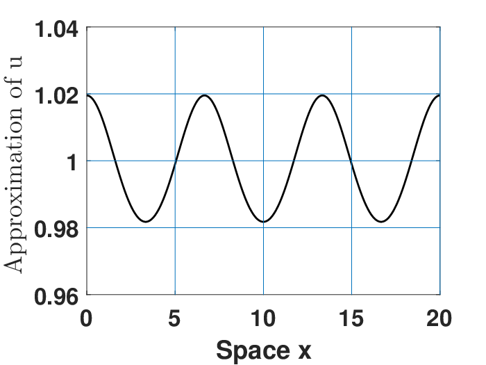
Next we numerically verify the asymptotic expressions of patterns in (3.15) and the selection mechanism of stable mode of steady states with small amplitudes (i.e., pattern solutions with small amplitudes) established in Proposition 3.1 and Theorem 3.2. By the analytical results, the stable wave mode is j=ia=6j=i_{a}=6, and thus the wave number of stationary pattern is 33, i.e., there are 33 peaks; moreover, the second-order approximation of the pattern solution in (3.15) is specified by

{u^ia≈1+ϵ​1.8883​cos⁡(0.9425​x)+ε2​(−1.7828+8.1736​cos⁡(1.885​x)),v^ia≈1+ϵ​cos⁡(0.9425​x)+ϵ2​(−1.7828+1.7952​cos⁡(1.885​x)),\displaystyle\left\{\begin{array}[]{ccc}\begin{aligned} &\widehat{u}_{i_{a}}\approx 1+\epsilon 1.8883\cos(0.9425x)+\varepsilon^{2}(-1.7828+8.1736\cos(1.885x)),\\ &\widehat{v}_{i_{a}}\approx 1+\epsilon\cos(0.9425x)+\epsilon^{2}(-1.7828+1.7952\cos(1.885x)),\end{aligned}\end{array}\right.

which is plotted in (a)(a) of Figure 2.

Refer to caption
Refer to caption

(a)                       (b)

Refer to caption
Refer to caption

(c)                       (d)

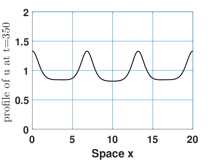
Figure 2: Comparison between the asymptotically approximate solution at O⁡(ϵ3)O(\epsilon^{3}) and numerical solutions of (2) with different values of parameter σ\sigma and different initial functions (u0,v0)(u_{0},v_{0}) which are perturbations of the spatially homogeneous steady state (1,1)(1,1). (a)(a) The stationary state (4). The other three pattern solutions are from simulations by directly integrating the model (1): (b)(b) (u0,v0)(u_{0},v_{0}) is the second-order approximation of (3.15) with j=3j=3 and a⁡(3)a(3) replaced by 1.5​a​(3)1.5a(3), σ=0.3\sigma=0.3; (c)(c) (u0,v0)(u_{0},v_{0}) is the second-order approximation of (3.15) with j=4j=4, σ=0.3\sigma=0.3; (d)(d) (u0,v0)(u_{0},v_{0}) is the second-order approximation of (3.15) with j=4j=4, σ=0.4\sigma=0.4.

In Figure 2, we show the comparison between the stationary state (4) predicted by the asymptotical analysis and the stationary states reached starting from different initial functions computed by numerically solving the system (2). It is seen that all the three simulation solutions (b)−(d)(b)-(d) are qualitatively in very good agreement with the analytical solution (a)(a), that is, all of them have three peaks (each of two boundary peaks evidently only counts as a half peak). The quantitative discrepancy is caused by ignoring the higher order terms of (4). It is also demonstrated that the bifurcation branch emanating from the maximum bifurcation point (i.e., the sixth one here) is stable since all the three simulation solutions (b)−(d)(b)-(d) tends to the steady state with wave mode j=6j=6 after about running time t=56,1200t=56,1200 and 350350, respectively. This verifies the stability criterion established in Proposition 3.1 and Theorem 3.2.

In Figure 3, we show the evolution of pattern starting from different initial locations. it is also observed that the sixth bifurcation branch is stable which is precisely predicted by our analytical results in Proposition 3.1 and Theorem 3.2. We see that solutions starting from different perturbation of the constant state (1,1)(1,1) finally reach the stationary pattern (i.e, the sixth bifurcation branch) which possesses 3 wave peaks (i.e., the wave mode j=6j=6).

Refer to caption
Refer to caption
Refer to caption

(i)                (ii)               (iii)

Figure 3: Pattern formation of model (2) for σ=0.32\sigma=0.32 and different initial functions (u0,v0)(u_{0},v_{0}). (i)(i) (u0,v0)(u_{0},v_{0}) is the second-order approximation of (3.15) with j=6j=6; (i​i)(ii) (u0,v0)(u_{0},v_{0}) is the second -order approximation of (3.15) with j=3j=3 and a⁡(3)a(3) replaced by 1.5​a​(3)1.5a(3); (i​i​i)(iii) (u0,v0)(u_{0},v_{0}) is the second-order approximation of (3.15) with j=4j=4 and a⁡(4)a(4) replaced by 1.2​a​(4)1.2a(4).

Figure 4 displays the process of pattern formation from the initial state to the stable steady state of Figure 3 (iii). The initial state has 22 wave peaks (i.e, the wave mode is j=4j=4), see the left-most one in the top line. Since the mode 44 steady state is unstable, as shown in the middle one of the top line, it is followed by the pattern having 44 wave peaks (i.e, j=8j=8) at about t=60t=60. Again due to the unstability of pattern with mode j=8j=8 predicted by Proposition 3.1, as we see from the left-most one in the bottom line, at about t=660t=660 merging phenomenon appears, then this solution transits to a stable state with mode j=6j=6 by reducing the 33 wave peaks in the interior of the domain to 22 ones. This transition is complete at about t=750t=750, and then the solution keeps the state with mode j=6j=6 that is stable. This once again confirms the stability criterion stated in Proposition 3.1 and Theorem 3.2.

Refer to caption
Figure 4: Numerical simulation of the transition from the given initial data to the stable state (u^6,v^6)(\widehat{u}_{6},\widehat{v}_{6}) of Figure 3 (iii). σ=0.32\sigma=0.32, the initial function (u0,v0)(u_{0},v_{0}) is the second-order approximation of (3.15) with j=4j=4 and a⁡(4)a(4) replaced by 1.2​a​(4)1.2a(4).

5 Conclusion

In this work, we present the detailed information of steady states near the trivial equilibrium and the global structure of the steady states of (2). The second-order approximation of non-constant steady states is also derived. Then by using the standard linear stability analysis and analytical technique, we further establish the stability criterion of the bifurcation branches. It is shown that the growth rate of bacteria σ\sigma substantially influences the dynamical behavior of the model (1). Particularly, under conditions (1.7) and (1.15) on the motility function r⁡(v)r(v), when the growth rate of bacteria is sufficiently large (i.e, for σ>σc\sigma>\sigma_{c}), the system will keep stabilization around the uniform state (1,1)(1,1); while for σ∈(0,σa)\sigma\in(0,\sigma_{a}), the pattern formation must occur, and thus the densities of bacteria and AHL always depend on their location. The principal wave mode of stationary pattern coincides with the admissible one which maximizes bifurcation values. The analytical results are corroborated by direct simulations of the underlying system (2) through different stages.

There are various interesting questions arising from our present analytical and numerical studies. The existence of non-constant steady states and the propagation of pattern in a large domain have been rigorously discussed and organized as a separate paper. It should be noticed that the question whether the pattern formation occurs in the cases when σ∈[σia,σc]\sigma\in[\sigma_{i_{a}},\sigma_{c}] or σ=0\sigma=0 has not been discussed yet. This question may be investigated by applying the approaches similar to that in [4, 11]. The global attractivity of non-constant steady state with the admissible wave mode still remains open. The bifurcating and emerging process in the pattern formation are numerically presented in Figures 3 and 4, but the mathematical behavior of the merging process is not well understood yet. All these questions are very interesting and challenging. We think it is worthwhile to explore theories and methods of solving them in the future.

Acknowledgement. This work was supported by the National Natural Science Foundation of China (No. 11671359) and the joint mobility project of the National Natural Science Foundation of China and Academy of Finland (No. 11811530145). M. Ma gratefully acknowledges the Department of Mathematics and Statistics at University of Turku for its hospitality and the help of its members during her stay there and the financial support of Academy of Finland. M. Vuorinen’s research at the Zhejiang Sci-tech University in April 2018 was supported by the National Natural Science Foundation of China (No. 11811530145) of Prof M. Ma.

References

  • [1] M. Crandall, and P. H. Rabinowitz, Bifurcation from simple eigenvalues, J. Functional Anal. 8 (1971) 321-340.
  • [2] X. Fu, L.-H. Tang, C. Liu, J. -D. Huang, T. Hwa, P. Lenz, Stripe formation in bacterial systems with density -suppressed motility, Physical review letters 108 (19) (2012) 198102.
  • [3] G. Gambino, M.C. Lombardo, M. Sammartino, Turing instability and traveling fronts for a nonlinear reaction-diffusion system with cross-diffusion, Math. Comput. Simulation 82 (2012) 1112-1132.
  • [4] G. Gambino, M.C. Lombardo, M. Sammartino, Pattern formation driven by cross-diffusion in 2d domain, Nonlinear Anal. RWA 14 (2013) 1755-1779.
  • [5] H. Y. Jin, Y. J. Kim, and Z. A. Wang, Boundedness, stabilization, and pattern formation driven by density- suppressed motility , SIAM J. Appl. Math., 78(3)(2018) 1632-1657.
  • [6] E. F. Keller and L. A. Segel, Model for chemotaxis, J. Theor. Biol. 30(2)(1971) 225-234.
  • [7] L. Kantorovich, G. Akilov, Functional Analysis in Normed Spaces, Macmillan, New York, 1964.
  • [8] C. Liu, X. Fu, L. Liu, X. Ren, C. K. Chau, S. Li, L. Xiang, H. Zeng, G.Chen, L.-H. Tang, et al., Sequential establishment of stripe patterns in an expanding cell population, Science 334 (6053) (2011) 238-241.
  • [9] Jaeduck Jang, Wei-Ming Ni and Moxun Tang, Global Bifurcation and Structure of Turing Patterns in the 1-D Lengyel-Epstein Model, Journal of Dynamics and Differential Equaation 16 (2)(2004) 297-320.
  • [10] M. Ma, Z. Wang, R. Peng, Stationary and non-stationary patterns of a reaction diffusion system with density-suppressed motility, Physica D: Nonlinear Phenomena, in press.
  • [11] M. Ma, M. Y. Gao, C. Q. Tong, and Y. Z. Han, Chemotaxis-driven pattern formation for a reaction-diffusion-chemotaxis model with volume-filling effect, Computers and Mathematics with Applications 72(2016) 1320-1340
  • [12] J. S. Roberge, D. Iron, and T. Kolokolnikov, Pattern formation in bacterial colonies with density-dependent diffusion, European Journal of Applied Mathematics, https://doi.org/10.1017/S0956792518000013Published online: 28 January 2018
  • [13] P. H. Rabinowitz, Some global results for nonlinear eigenvalue problems, J. Functional Anal. 7 (1971) 487-513.
  • [14] Y. Tao and M. Winkler, Effects of signal-dependent motilities in a Keller-Segel-type reaction-diffusion system, Math. Models Meth. Appl. Sci. 27(19)(2017) 1645-1683.
  • [15] I. Takagi, Point-condensation for a reaction-diffusion system, J. Diff. Eqns 61(1986) 208-249.
  • [16] P. Xia, Y. Han, J. Tao, M. Ma, Existence and metastability of non-constant steady states in a Keller-Segel model with density-suppressed motility, Mathematics in Applied Sciences and Engineering, in press.
  • [17] Nishiura. Y, Global structure of bifurcating solutions of some reaction-diffusion systems, SIAM J. Math. Anal. 13(1982) 555-593.
  • [18] C. Yoon and Y.-J. Kim, Global existence and aggregation in a Keller-Segel model with Fokker-Planck diffusion, Acta Application Mathematics 149 (2017) 101-123.
  • [19] C. Yoon and Y.-J. Kim, Bacterial chemotaxis without gradient sensing, J. Math. Biol. 70(2015) 1359-1380.

FILE: MXversion28.tex