Functional Transparency for Structured Data: a Game-Theoretic Approach

There are many ways to use a witness function $g\in\mathcal{G}$ to guide the predictor $f$ by means of discrepancy measures. However, since the witness functions can be weak such as linear functions, we cannot expect that a reasonable predictor would agree to it globally. Instead, we make a slight generalization to enforce this criterion only locally, over different sets of neighborhoods. To this end, we define local transparency by measuring how close $f$ is to the family $\mathcal{G}$ over a local neighborhood $\mathcal{B}(x_{i})\subset\mathcal{X}$ around an observed point $x_{i}$. One straightforward instantiation of such a neighborhood $\mathcal{B}_{\epsilon}({x_{i}})$ in temporal domain will be simply a local window of points $\{x_{i-\epsilon},\dots,x_{i+\epsilon}\}$. Our resulting local discrepancy measure is

The summation can be replaced by an integral when a continuous neighborhood is used. The minimizing witness function, $\hat{g}_{x_{i}}$, is indexed by the point $x_{i}$ around which it is estimated; depending on the function $f$, the minimizing witness can change from one neighborhood to another. If we view the minimization problem game-theoretically, $\hat{g}_{x_{i}}$ is the best response strategy of the local witness around $x_{i}$.

The local discrepancy measure can be incorporated into an overall estimation criterion in many ways so as to guide the predictor towards the desired functional form. This guidance can be offered as a uniform constraint with a permissible $\delta$-margin, as an additive symmetric penalty, or defined asymmetrically as a game theoretic penalty where the information sets for the predictor and the witness are no longer identical. We consider each of these in turn.

Uniform criterion. A straightforward formulation is to confine $f$ to remain within a margin $\delta$ of the best fitting witness for every local neighborhood. Assume that a primal loss $\mathcal{L}(\cdot,\cdot)$ is given for a learning task. The criterion imposes the $\delta$-margin constraint uniformly as

We assume that the optimal $g$ with respect to each constraint may be efficiently found due to the simplicity of $\mathcal{G}$ and the regularity of $d(\cdot,\cdot)$. We also assume that the partial derivatives with respect to $f$, for fixed witnesses, can be computed straightforwardly under sufficiently regular $\mathcal{L}(\cdot,\cdot)$ in a Lagrangian form. In this case, we can solve for $f$, local witnesses, and the Lagrange multipliers using the mirror-prox algorithm (Nemirovski 2004).

The hard constraints in the uniform criterion will lead to strict transparency guarantees. However, the effect may be undesirable in some cases where the observed data (hence the predictor) do not agree with the witness in all places. The resulting loss of performance may be too severe. As an alternative, we can enforce the agreement with local witnesses to be small in aggregate across neighborhoods.

Symmetric game. We define an additive, unconstrained, symmetric criterion to smoothly trade off between performance and transparency. The resulting objective is

To illustrate the above idea, we generate a synthetic dataset to show a neighborhood in Figure 2(a) with an unconstrained piecewise linear predictor $f\in\mathcal{F_{\text{piecewise linear}}}$ in Figure 2(b). Clearly, $f$ does not agree with a linear witness within this neighborhood. However, when we solve for $f$ together with a linear witness $g_{x_{i}}\in\mathcal{G}_{\text{linear}}$ as in Figure 2(c), the resulting function has a small residual deviation from $\mathcal{G}_{\text{linear}}$, more strongly adhering to the linear functional class while still closely tracking the observed data. Figure 2(d) shows the flexibility of our framework where a very different functional behavior can be induced by changing the functional class for the witness.

Asymmetric game. Solving the symmetric criterion can be computationally inefficient since the predictor is guided by its deviation from each of the local witness on all points within each of the local neighborhoods. Moreover, the predictor value at any point $x_{i}$ is subject to potentially conflicting regularization terms across the neighborhoods, which is undesirable. The inner summation in Eq. (3) may involve different sizes of neighborhoods $\mathcal{B}(x_{i})$ (e.g., end-point boundary cases) and this makes it more challenging to parallelize the computation.

We would like to impose even functional regularization at every $f(x_{i})$ based on how much the value deviates from the witness associated with the local region $\mathcal{B}(x_{i})$. This approach leads to an asymmetric co-operative formulation, where the information sets for the predictor $f$ and local witnesses $g_{x_{i}}$ differ. Specifically, the local best-response witness $\hat{g}_{x_{i}}$ is chosen to minimize the local discrepancy as in Eq. (1), and thus depends on $f$ values within the whole region; in contrast, the predictor $f$ only receives feedback in terms of the resulting deviation at $x_{i}$, only seeing $\hat{g}_{x_{i}}(x_{i})$. From the point of view of the predictor $f$, the best response strategy is obtained by minimizing

To train the proposed method, we perform alternating updates for $f(\cdot)$ and $\hat{g}_{x_{i}}(\cdot)$ on their respective criteria.

We consider here the effectiveness of regularization in relation to the neighborhood size and establish fixed point equations for the predictor under the three estimation criteria. For simplicity, we assume $\mathcal{X}=\mathbb{R}^{d}$ and $\mathcal{Y}=\mathbb{R}$, but the results are generalizable to our examples in §4. All the proofs are in Appendix A.

Neighborhood size. The formulation involves a key trade-off between the size of the region where the function should be simple and the overall accuracy achieved by the predictor. When the neighborhood is too small, local witnesses become perfect, inducing no regularization on $f$. Thus the size of the region is a key parameter. A neighborhood size is sufficient if the witness class $\mathcal{G}$ cannot readily overfit $f$ values within the neighborhood. Formally,

A trivial example is when $\mathcal{G}$ is the constant class, a neighborhood size $m$ is effective if $m>1$. Note that the neighborhood $\mathcal{B}$ in the above definition can be any finite collection of points $\mathcal{B}(\cdot)$. For example, the points in the neighborhood induced by a temporal window $\{x_{i-\epsilon},\dots,x_{i+\epsilon}\}$ need not remain in a small $\ell_{p}$-norm ball.

For linear models and decision trees, we have

• •

  $d+1$ is the tight lower bound on the effective neighborhood size for the linear class.

• •

  $2^{k}+1$ is the tight lower bound on the effective neighborhood size for the decision tree class with depth bounded by $k$.

When the sample sizes within the neighborhoods fall below such bounds, regularization can still be useful if the witness class is not uniformly flexible or if the algorithm for finding the witness is limited (e.g., greedy algorithm for decision trees).

Equilibrium solutions. The symmetric game constitutes a standard minimization problem, but the existence or uniqueness of equilibria under the asymmetric game are not obvious. Our main results in this section make the following assumptions.

• (A1) the predictor $f$ is unconstrained.

• (A2) both the loss and deviation are squared errors.

• (A3) $|\mathcal{B}(x_{i})|=m,\forall x_{i}\in\mathcal{D}_{x}$.

• (A4) $x_{j}\in\mathcal{B}(x_{i})\implies x_{i}\in\mathcal{B}(x_{j}),\forall x_{i},x_{j}\in\mathcal{D}_{x}$.

• (A5) $\cup_{x_{i}\in\mathcal{D}_{x}}\mathcal{B}(x_{i})=\mathcal{D}_{x}$.

We note that (A3) and (A4) are not technically necessary but simplify the presentation. We denote the predictor in the uniform criterion (Eq. (2)), the symmetric game (Eq. (3)), and the asymmetric game (Eq. (4)) as $f_{U}$, $f_{S}$, and $f_{A}$, respectively. We use $X_{i}\in\mathbb{R}^{m\times d}$ to denote the neighborhood $\mathcal{B}(x_{i})=\{x^{\prime}_{1},\dots,x^{\prime}_{m}\}$ ($X_{i}=[x^{\prime}_{1},\dots,x^{\prime}_{m}]^{\top}$), and $f(X_{i})\in\mathbb{R}^{m}$ to denote the vector $[f(x^{\prime}_{1}),\dots,f(x^{\prime}_{m})]^{\top}$. $X_{j}^{\dagger}$ denotes the pseudo-inverse of $X_{j}$. Then we have

The equilibrium in the linear class is not unique when the witness is not fully determined in a neighborhood due to degeneracy. To avoid these cases, we can use Ridge regression to obtain a stable equilibrium (proved also in Appendix).

A special case of Theorem 2 is when $x_{i}=[1],\forall x_{i}\in\mathcal{D}_{x}$, which effectively yields the equilibrium result for the constant class; we found it particularly useful to understand the similarity between the two games in this scenario. Concretely, each $(X^{\dagger}_{j}f(X_{j}))^{\top}x_{i}$ becomes equivalent to $\frac{1}{m}\sum_{x_{k}\in\mathcal{B}(x_{j})}f(x_{k})$. As a result, the solution for both the symmetric and asymmetric game induce the optimal predictors as recursive convolutional averaging of neighboring points with the same decay rate ${\lambda}/({1+\lambda})$, while the convolutional kernel evolves twice as fast in the symmetric game than in the asymmetric game.

Next, we show that the hard uniform constraint criterion yields a very different equilibrium.

A noticeable difference from the games is that, under uniform criterion, the optimal predictor $f^{*}_{U}(x_{i})$ may faithfully output the actual label $y_{i}$ if the functional constraint is satisfied, while the functional constraints are translated into a “convolutional” operator in the games.

Efficient computation. We also analyze ways of accelerating the computation required for solving the symmetric game. An equivalent criterion is given by

The result is useful when training $f$ on GPU and $\hat{g}_{x_{i}}$ is solved analytically on CPU. Compared to a for-loop to handle different neighborhood sizes for Eq. (3) on the GPU, computing a summarized feedback as in Lemma 4 on CPU is more efficient (and easier to implement).

Discussion We investigated here discrete neighborhoods and they are suitable also for structured data as in the experiments. The method itself can be generalized to continuous neighborhoods with an additional difficulty: the exact computation and minimization of functional deviation between the predictor and the witness in such neighborhood is in general intractable. We may apply results from learning theory (e.g., (Shamir 2015)) to bound the (generalization) gap between the deviation computed by finite samples from the continuous neighborhood and the actual deviation under a uniform probability measure.

The basic idea of co-operative modeling extends naturally to conditional sequence generation over longer periods. Broadly, the mechanism allows us to inspect the temporal progression of sequences on a longer term basis.

Given an observation sequence $x_{1},\dots,$ $x_{t}\in\mathbb{R}^{c}$, the goal is to estimate probability $p(x_{t+1:T}|x_{1:t})$ over future events $x_{t+1},\dots,$ $x_{T}\in\mathbb{R}^{c}$, typically done via maximum likelihood. For brevity, we use $x_{1:i}$ to denote $x_{1},\dots,x_{i}$. We model the conditional distribution of $x_{i+1}$ given ${x}_{1:i}$ as a multivariate Gaussian distribution with mean $\mu(x_{1:i})$ and covariance $\Sigma(x_{1:i})$, both parametrized as recurrent neural networks. Each local witness model $g_{{x}_{1:i}}(\cdot)$ is estimated based on the neighborhood $\mathcal{B}(x_{1:i}):=\{{x}_{1:i-\epsilon},\dots,{x}_{1:i+\epsilon}\}$ with respect to the mean function $\mu(\cdot)$. A natural choice would be a $K$-order Markov autoregressive (AR) model with an $\ell_{2}$ deviation loss as:

where $\theta_{k}\in\mathbb{R}^{c\times c},\forall k>0$ and $\theta_{0}\in\mathbb{R}^{c}$. The AR model admits an analytical solution similar to linear regression.

The models discussed in §3 can be instantiated on highly-structured data, such as molecules, too. These are usually represented as a graph $\mathcal{M}=(\mathcal{V},\mathcal{E})$ whose nodes encode the atom types and edges encode the chemical bonds. Such representation enables the usage of recent graph convolutional networks (GCNs) (Dai et al. 2016; Lei et al. 2017) as the predictor $f$. As it is hard to realize a simple explanation on the raw graph representation, we exploit an alternative data representation for the witness model; we leverage depth-bounded decision trees that take as input Morgan fingerprints (Rogers & Hahn 2010) $x(\mathcal{M})$, which are vector representations for the binary existence of a chemical substructures in a molecule (e.g., the nodes in Fig. 1).

The neighborhood $\mathcal{B}(\mathcal{M})$ includes molecules $\{\mathcal{M}^{\prime}\}$ with Tanimoto similarity greater than $0.6$, automatically constructed through matching molecular pair analysis (Griffen et al. 2011). Here we use a multi-label binary classification task as an example, and adopt a cross-entropy loss for each label axis for simplicity. At each neighborhood $\mathcal{B}(\mathcal{M})$, we construct a witness decision tree $g$ that minimizes the total variation (TV) from the predictor as

We note that Eq. (6) is an upper bound and efficient alternative to fitting a tree for each label axis independently.

Our approach can be further applied to learn transparent latent graph representations by variational autoencoders (VAEs) (Kingma & Welling 2013; Jin et al. 2018). Concretely, given a molecular graph $\mathcal{M}=(\mathcal{V},\mathcal{E})$, the VAE encoder $q$ outputs the approximated posterior $z_{\mathcal{M}}\sim\mathcal{N}(\mu_{\mathcal{M}},\Sigma_{\mathcal{M}})$ over the latent space, where $z_{\mathcal{M}}$ is the continuous representation of molecule $\mathcal{M}$. Following common practice, $\Sigma_{\mathcal{M}}$ is restricted to be diagonal. The VAE decoder then reconstructs the molecule $\mathcal{M}$ from its probabilistic encoding $z_{\mathcal{M}}$. Our goal here is to guide the behavior of the neural encoder $q$ such that the derivation of (probabilistic) $z_{\mathcal{M}}$ can be locally explained by a decision tree.

We adopt the same setting for the witness function and neighborhoods as in §4.2, except that the local decision tree $g$ now outputs a joint normal distribution with parameters $[\widehat{\mu}_{\mathcal{M}},\widehat{\Sigma}_{\mathcal{M}}]$. To train the encoder, we extend the original VAE objective $\mathcal{L}^{\mathrm{VAE}}$ with a local deviation loss $\mathcal{L}^{\mathcal{G}_{\text{tree}}}$ defined on the KL divergence between the VAE posterior $q(\mathcal{M})=\mathcal{N}(\mu_{\mathcal{M}},\Sigma_{\mathcal{M}})$ and witness posterior $g(x(\mathcal{M}))=\mathcal{N}(\widehat{\mu}_{\mathcal{M}},\widehat{\Sigma}_{\mathcal{M}})$ at each neighborhood as

The VAE is trained to maximize $\mathcal{L}^{\mathrm{VAE}}+\lambda\cdot\mathcal{L}^{\mathcal{G}_{\text{tree}}}$. For ease of implementation, we asymmetrically estimate each decision tree $g$ with mean squared error between the vectors $[\mu_{\mathcal{M}},\Sigma_{\mathcal{M}}]$ and $[\widehat{\mu}_{\mathcal{M}},\widehat{\Sigma}_{\mathcal{M}}]$.

We conduct experiments on molecular toxicity prediction on the Tox21 dataset from MoleculeNet benchmark (Wu et al. 2018b), which contains 12 binary labels and $7,831$ molecules. The labels are very unbalanced; the fraction of the positive label is between $16.15\%$ and $3.51\%$ among the 12 labels. We use GCN as the predictor and decision trees as the witnesses as in §4.2. The neighborhood sizes $m$ of about $60\%$ of the molecules are larger than $2$, whose median and maximum are $59$ and $300$, respectively. Since each neighborhood has a different size $m$, we set the maximum tree depth as $\max\{\lceil\log_{2}(m)\rceil-1,1\}$ for each neighborhood, which ensures that the corresponding size $m$ is effective for $m>2$ (see Definition 1). More details are in Appendix B.

Evaluation Measures: For all the measures, the results are averaged across the label axes.

(1) Performance: For the predictor, we compare its predictions with respect to the labels in AUC, denoted as AUC$(f,y)$. As each local witness $\hat{g}_{\mathcal{M}}(x(\mathcal{M}))$ also realizes a function of $\mathcal{M}$, it is also evaluated against the labels in AUC, denoted as AUC$(\hat{g}_{\mathcal{M}},y)$.

(2) Transparency: As labels are unavailable for testing data in practice, it is more realistic to measure the similarity between the predictor and the local witnesses to understand the validity of the explanations derived from the decision trees $\mathcal{G}$. To this end¹¹ 1 Since the predictor probability can be scaled arbitrarily to minimize the TV from decision trees without affecting performance, using TV to measure transparency as used in training is not ideal., we generalize the AUC criterion for continuous labels for $N$ references $y$ and predictions $y^{\prime}$ as

The proposed score has the same pairwise interpretation as AUC, recovers AUC when $y$ is binary, and is normalized to $[0,1]$. Locally, we measure the criterion for the local witnesses with respect to the predictor in each testing neighborhood as the local deviation, where the average result is denoted as $\text{AUC}_{\mathcal{B}}(\hat{g}_{\mathcal{M}},f)$. Globally, the criterion is also validated among the testing data, denoted as $\text{AUC}_{\mathcal{D}}(\hat{g}_{\mathcal{M}},f)$.

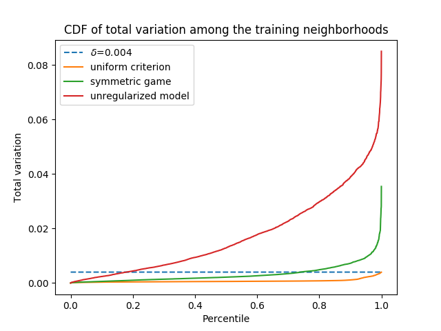
The results with the uniform and symmetric criteria are shown in Table 1. A baseline vanilla decision tree, with depth tuned between $2$ and $30$, yields 0.617 in $\text{AUC}(f,y)$. Compared to $\textsc{Game}_{\text{sym}}$, the local deviation in $\textsc{Game}_{\text{unif}}$ is marginally improved due to the strict constraint at the cost of severe performance loss. We investigate the behaviors in training neighborhoods and find that $\textsc{Game}_{\text{sym}}$ exhibits a tiny fraction of high deviation losses, allowing the model to behave more flexibly than the strictly constrained $\textsc{Game}_{\text{unif}}$ (see Figure 5 in Appendix B). In terms of performance, our $\textsc{Game}_{\text{sym}}$ model is superior to the Deep model in both the predictor and local witnesses. When comparing the witnesses to the predictor, locally and globally, the Game models significantly improve the transparency from the Deep model. The local deviation should be interpreted relatively since the tree depth inherently prevents local overfitting.

We visualize the resulting witness trees in Figure 1 under the same transparency constraint: for a local neighborhood, we grow the witness tree for the Deep model until the local transparency in $\text{AUC}_{\mathcal{B}}$ is comparable to the $\textsc{Game}_{\text{sym}}$ model. For explaining the same molecule, the tree for the Deep model is deeper and extremely unbalanced. Since a Morgan fingerprint encodes the existence of a substructure of molecule graphs, an unbalanced tree focusing on the left branch (non-existence of a substructure) does not capture much generality. Hence, the explanation of the Deep model does not provide as much insight as our $\textsc{Game}_{\text{sym}}$ model.

Here we do an analysis on the tree depth constraint for the witness model, as a shallower tree is easier to interpret, but more challenging to establish transparency due to the restricted complexity. To this end, we revise the depth constraint to $\max\{\lceil\log_{2}(m)\rceil-1+\Delta,1\}$ during training and testing, and vary $\Delta\in\{-3,\dots,0\}$. All the resulting Game models outperform the Deep models in AUC$(f,y)$, and we report the transparency score in terms of $\text{AUC}_{\mathcal{D}}(\hat{g}_{\mathcal{M}},f)$ in Table 2. Even when $\Delta=-3$, the witness trees in our Game model still represent the predictor more faithfully than those in the Deep model with $\Delta=0$.

We next validate our approach on a physical component modeling task with the bearing dataset from NASA (Lee et al. 2016), which records 4-channel acceleration data on 4 co-located bearings. We divide the sequence into disjoint subsequences, resulting in $200,736$ subsequences. Since the dataset exhibits high frequency periods of 5 points and low frequency periods of 20 points, we use the first $80$ points in an sequence to forecast the next $20$. We parametrize $\mu(\cdot)$ and $\Lambda(\cdot)$ jointly by stacking $1$ layer of CNN, LSTM, and $2$ fully connected layers. We set the neighborhood radius $\epsilon$ to $9$ such that the witnesses are fit with completely different data for the beginning and the end of the sequence. The Markov order $K$ is set to $2$ to ensure the effectiveness of the neighborhood sizes. More details are in Appendix C.

Evaluation involves three different types of errors: 1) ‘error’ is the root mean squared error (RMSE) between greedy autoregressive generation and the ground truth, 2) ‘deviation’ is RMSE between the predictor $\mu(x_{1:i})$ and the witness $\hat{g}_{x_{1:i}}(x_{1:i})$, and 3) ‘TV’ is the average total variation of witness $\hat{g}_{x_{1:i}}$ parameters $[{\theta},{\theta}_{0}]$ between every two consecutive time points. Since the deviation and error are both computed on the same space in RMSE, the two measures are readily comparable. For testing, the witnesses are estimated based on the autoregressive generative trajectories.

We present the results in Table 3 to study the impact of the game coefficient $\lambda$ and the symmetry of the games. The trends in the measures are quite monotonic on $\lambda$: with an increasing $\lambda$, the model gradually operates toward the AR family with lower deviation and TV but higher error. When $\lambda=0.1$, the Game models are more accurate than the Deep model ($\lambda=0$) due to the regularization effect. Given the same hyper-parameters, marginally lower deviation in the symmetric game than in the asymmetric game confirms our analysis about the similarity between the two. In practice, the asymmetric game is more efficient and substantially easier to implement than the symmetric game. Indeed, the training time is $20.6$ sequences/second for the asymmetric game, and $14.6$ sequences/second for the symmetric game. If we use the formula in Lemma 4, the symmetric game can be accelerated to $20.4$ sequences/second, but the formula does not generalize to other deviation losses.

We visualize the witnesses with their parameters $[\theta_{0},\theta]$ along the autoregressive generative trajectories in Figure 3. The stable functional patterns of the Game model as reflected by $\theta$, before and after the $9^{\text{th}}$ point, highlight not only close local alignments of the predictor and the AR family (being constant vectors across columns) but also flexible variation of functional properties on the predictor across regions. In contrast, the Deep model yields unstable linear coefficients, and relies more on offsets/biases $\theta_{0}$ than the Game model, while the linear weights are more useful for grounding the coordinate relevance for interpretability. Finally, we remark that despite the uninterpretable nature of temporal signals, the functional pattern reflected by the linear weights as shown here yields a simple medium to understand its behavior. Due to space limitation, the additional analysis and visualization are included in Appendix C.

Finally, we validate our approach on learning representations for molecules with VAEs, where we use the junction tree VAE (Jin et al. 2018) as an example. Here the encoders of VAEs, with and without the guidance of local decision trees as in §4.3, are denoted as Deep and Game, respectively. The models are trained on the ZINC dataset (Sterling & Irwin 2015) containing 1.5M molecules, and evaluated on a test set with 20K molecules. We measure the performance in terms of the evidence lower bound (ELBO) over the test set. Here we consider two scenarios: the ELBO using the raw latent representations from the original neural encoder, and using the interpreted latent representations generated by locally fitted decision trees. The average deviation loss in KL divergence $\mathcal{L}^{\mathcal{G}_{\text{tree}}}$, defined in §4.3, over the testing neighborhoods is also evaluated.

The results are shown in Table 4. Our Game model performs consistently better under all the metrics. Figure 4 shows an example of how our decision tree explains the local neighborhood of a molecule. We found most of the substructures selected by the decision tree occur in the side chains outside of Bemis-Murcko scaffold (Bemis & Murcko 1996). This shows the variation in the latent representation mostly reflects the local changes in the molecules, which is expected since changes in the scaffold typically lead to global changes such as chemical property changes.

References

- Abadi et al. (2016) Abadi, M., Barham, P., Chen, J., Chen, Z., Davis, A., Dean, J., Devin, M., Ghemawat, S., Irving, G., Isard, M., et al. Tensorflow: a system for large-scale machine learning. In OSDI, volume 16, pp. 265–283, 2016.
- Al-Shedivat et al. (2017) Al-Shedivat, M., Dubey, A., and Xing, E. P. Contextual explanation networks. arXiv preprint arXiv:1705.10301, 2017.
- Alvarez-Melis & Jaakkola (2018a) Alvarez-Melis, D. and Jaakkola, T. Towards robust interpretability with self-explaining neural networks. In Advances in Neural Information Processing Systems, pp. 7786–7795, 2018a.
- Alvarez-Melis & Jaakkola (2017) Alvarez-Melis, D. and Jaakkola, T. S. A causal framework for explaining the predictions of black-box sequence-to-sequence models. Proceedings of EMNLP, 2017.
- Alvarez-Melis & Jaakkola (2018b) Alvarez-Melis, D. and Jaakkola, T. S. On the robustness of interpretability methods. arXiv preprint arXiv:1806.08049, 2018b.
- Arjovsky et al. (2017) Arjovsky, M., Chintala, S., and Bottou, L. Wasserstein gan. arXiv preprint arXiv:1701.07875, 2017.
- Arras et al. (2017) Arras, L., Horn, F., Montavon, G., Müller, K.-R., and Samek, W. ” What is relevant in a text document?”: An interpretable machine learning approach. PloS one, 12(8):e0181142, 2017.
- Bellemare et al. (2017) Bellemare, M. G., Danihelka, I., Dabney, W., Mohamed, S., Lakshminarayanan, B., Hoyer, S., and Munos, R. The cramer distance as a solution to biased wasserstein gradients. arXiv preprint arXiv:1705.10743, 2017.
- Bemis & Murcko (1996) Bemis, G. W. and Murcko, M. A. The properties of known drugs. 1. molecular frameworks. Journal of medicinal chemistry, 39(15):2887–2893, 1996.
- Cisse et al. (2017) Cisse, M., Bojanowski, P., Grave, E., Dauphin, Y., and Usunier, N. Parseval networks: Improving robustness to adversarial examples. arXiv preprint arXiv:1704.08847, 2017.
- Citron & Pasquale (2014) Citron, D. K. and Pasquale, F. The scored society: due process for automated predictions. Wash. L. Rev., 89:1, 2014.
- Dai et al. (2016) Dai, H., Dai, B., and Song, L. Discriminative embeddings of latent variable models for structured data. In International Conference on Machine Learning, pp. 2702–2711, 2016.
- Ganin et al. (2016) Ganin, Y., Ustinova, E., Ajakan, H., Germain, P., Larochelle, H., Laviolette, F., Marchand, M., and Lempitsky, V. Domain-adversarial training of neural networks. The Journal of Machine Learning Research, 17(1):2096–2030, 2016.
- Ghorbani et al. (2019) Ghorbani, A., Abid, A., and Zou, J. Interpretation of neural networks is fragile. AAAI, 2019.
- Goodfellow et al. (2014) Goodfellow, I., Shlens, J., and Szegedy, C. Explaining and harnessing adversarial examples. 12 2014.
- Griffen et al. (2011) Griffen, E., Leach, A. G., Robb, G. R., and Warner, D. J. Matched molecular pairs as a medicinal chemistry tool: miniperspective. Journal of medicinal chemistry, 54(22):7739–7750, 2011.
- Gulrajani et al. (2017) Gulrajani, I., Ahmed, F., Arjovsky, M., Dumoulin, V., and Courville, A. C. Improved training of wasserstein gans. In Advances in Neural Information Processing Systems, pp. 5767–5777, 2017.
- He et al. (2016) He, K., Zhang, X., Ren, S., and Sun, J. Deep residual learning for image recognition. In Proceedings of the IEEE conference on computer vision and pattern recognition, pp. 770–778, 2016.
- Helfrich et al. (2017) Helfrich, K., Willmott, D., and Ye, Q. Orthogonal recurrent neural networks with scaled cayley transform. arXiv preprint arXiv:1707.09520, 2017.
- Huang et al. (2017) Huang, G., Liu, Z., Van Der Maaten, L., and Weinberger, K. Q. Densely connected convolutional networks. In CVPR, volume 1, pp. 3, 2017.
- Jin et al. (2018) Jin, W., Barzilay, R., and Jaakkola, T. Junction tree variational autoencoder for molecular graph generation. arXiv preprint arXiv:1802.04364, 2018.
- Kingma & Welling (2013) Kingma, D. P. and Welling, M. Auto-encoding variational bayes. arXiv preprint arXiv:1312.6114, 2013.
- Kovačević et al. (2008) Kovačević, J., Chebira, A., et al. An introduction to frames. Foundations and Trends® in Signal Processing, 2(1):1–94, 2008.
- Lakkaraju et al. (2016) Lakkaraju, H., Bach, S. H., and Leskovec, J. Interpretable decision sets: A joint framework for description and prediction. In Proceedings of the 22nd ACM SIGKDD international conference on knowledge discovery and data mining, pp. 1675–1684. ACM, 2016.
- (25) Lee, G.-H., Alvarez-Melis, D., and Jaakkola, T. S. Game-theoretic interpretability for temporal modeling. The 5th Workshop on Fairness, Accountability, and Transparency in Machine Learning (FAT/ML 2018) at ICML 2018. URL https://arxiv.org/pdf/1807.00130.pdf.
- Lee et al. (2016) Lee, J., Qiu, H., Yu, G., Lin, J., and Rexnord Technical Services (2007). IMS, U. o. C. Bearing data set. NASA Ames Prognostics Data Repository (http://ti.arc.nasa.gov/project/prognostic-data-repository), NASA Ames Research Center, Moffett Field, CA, 7(8), 2016.
- Lei et al. (2016) Lei, T., Barzilay, R., and Jaakkola, T. Rationalizing Neural Predictions. In EMNLP 2016, Proceedings of the 2016 Conference on Empirical Methods in Natural Language Processing, pp. 107–117, 2016. URL http://arxiv.org/abs/1606.04155.
- Lei et al. (2017) Lei, T., Jin, W., Barzilay, R., and Jaakkola, T. Deriving neural architectures from sequence and graph kernels. arXiv preprint arXiv:1705.09037, 2017.
- Mahendran & Vedaldi (2015) Mahendran, A. and Vedaldi, A. Understanding deep image representations by inverting them. Proceedings of the IEEE conference on computer vision and pattern recognition, 2015.
- Miller & Hardt (2018) Miller, J. and Hardt, M. When recurrent models don’t need to be recurrent. arXiv preprint arXiv:1805.10369, 2018.
- Mroueh et al. (2018) Mroueh, Y., Li, C.-L., Sercu, T., Raj, A., and Cheng, Y. Sobolev gan. International Conference on Learning Representations, 2018.
- Müller (1997) Müller, A. Integral probability metrics and their generating classes of functions. Advances in Applied Probability, 29(2):429–443, 1997.
- Nemirovski (2004) Nemirovski, A. Prox-method with rate of convergence o (1/t) for variational inequalities with lipschitz continuous monotone operators and smooth convex-concave saddle point problems. SIAM Journal on Optimization, 15(1):229–251, 2004.
- Pasquale (2015) Pasquale, F. The black box society: The secret algorithms that control money and information. Harvard University Press, 2015.
- Pedregosa et al. (2011) Pedregosa, F., Varoquaux, G., Gramfort, A., Michel, V., Thirion, B., Grisel, O., Blondel, M., Prettenhofer, P., Weiss, R., Dubourg, V., et al. Scikit-learn: Machine learning in python. Journal of machine learning research, 12(Oct):2825–2830, 2011.
- Quinlan (2014) Quinlan, J. R. C4. 5: programs for machine learning. Elsevier, 2014.
- Ribeiro et al. (2016) Ribeiro, M. T., Singh, S., and Guestrin, C. ”Why Should I Trust You?”: Explaining the Predictions of Any Classifier. In Proceedings of the 22Nd ACM SIGKDD International Conference on Knowledge Discovery and Data Mining, pp. 1135–1144, New York, NY, USA, 2016. ACM. ISBN 978-1-4503-4232-2. doi: 10.1145/2939672.2939778. URL http://arxiv.org/abs/1602.04938http://doi.acm.org/10.1145/2939672.2939778.
- Rogers & Hahn (2010) Rogers, D. and Hahn, M. Extended-connectivity fingerprints. Journal of chemical information and modeling, 50(5):742–754, 2010.
- Selvaraju et al. (2016) Selvaraju, R. R., Cogswell, M., Das, A., Vedantam, R., Parikh, D., and Batra, D. Grad-cam: Visual explanations from deep networks via gradient-based localization. https://arxiv. org/abs/1610.02391 v3, 7(8), 2016.
- Shamir (2015) Shamir, O. The sample complexity of learning linear predictors with the squared loss. The Journal of Machine Learning Research, 16(1):3475–3486, 2015.
- Silver et al. (2016) Silver, D., Huang, A., Maddison, C. J., Guez, A., Sifre, L., Van Den Driessche, G., Schrittwieser, J., Antonoglou, I., Panneershelvam, V., Lanctot, M., et al. Mastering the game of go with deep neural networks and tree search. nature, 529(7587):484, 2016.
- Sterling & Irwin (2015) Sterling, T. and Irwin, J. J. Zinc 15–ligand discovery for everyone. Journal of chemical information and modeling, 55(11):2324–2337, 2015.
- Vaswani et al. (2017) Vaswani, A., Shazeer, N., Parmar, N., Uszkoreit, J., Jones, L., Gomez, A. N., Kaiser, Ł., and Polosukhin, I. Attention is all you need. In Advances in Neural Information Processing Systems, pp. 5998–6008, 2017.
- Wu et al. (2018a) Wu, M., Hughes, M. C., Parbhoo, S., Zazzi, M., Roth, V., and Doshi-Velez, F. Beyond sparsity: Tree regularization of deep models for interpretability. In Proceedings of the Thirty-Second AAAI Conference on Artificial Intelligence, New Orleans, Louisiana, USA, February 2-7, 2018, 2018a. URL https://www.aaai.org/ocs/index.php/AAAI/AAAI18/paper/view/16285.
- Wu et al. (2018b) Wu, Z., Ramsundar, B., Feinberg, E. N., Gomes, J., Geniesse, C., Pappu, A. S., Leswing, K., and Pande, V. Moleculenet: a benchmark for molecular machine learning. Chemical science, 9(2):513–530, 2018b.
- Zhao et al. (2017) Zhao, M., Yue, S., Katabi, D., Jaakkola, T. S., and Bianchi, M. T. Learning sleep stages from radio signals: a conditional adversarial architecture. In International Conference on Machine Learning, pp. 4100–4109, 2017.
Appendix A Proofs
Our main results in this section make the following assumptions.
-
(A1) the predictor is unconstrained.