Learning a Deep ConvNet for Multi-label Classification with Partial Labels

Thibaut Durand Nazanin Mehrasa Greg Mori Affiliation: Borealis AI Simon Fraser University Email: {tdurand,nmehrasa}@sfu.ca mori@cs.sfu.ca

Abstract

Deep ConvNets have shown great performance for single-label image classification (e.g. ImageNet), but it is necessary to move beyond the single-label classification task because pictures of everyday life are inherently multi-label. Multi-label classification is a more difficult task than single-label classification because both the input images and output label spaces are more complex. Furthermore, collecting clean multi-label annotations is more difficult to scale-up than single-label annotations. To reduce the annotation cost, we propose to train a model with partial labels i.e. only some labels are known per image. We first empirically compare different labeling strategies to show the potential for using partial labels on multi-label datasets. Then to learn with partial labels, we introduce a new classification loss that exploits the proportion of known labels per example. Our approach allows the use of the same training settings as when learning with all the annotations. We further explore several curriculum learning based strategies to predict missing labels. Experiments are performed on three large-scale multi-label datasets: MS COCO, NUS-WIDE and Open Images.

1 Introduction

Recently, Stock and Cisse Stock2018 presented empirical evidence that the performance of state-of-the-art classifiers on ImageNet Russakovsky2015 is largely underestimated – much of the reamining error is due to the fact that ImageNet’s single-label annotation ignores the intrinsic multi-label nature of the images. Unlike ImageNet, multi-label datasets (e.g. MS COCO Lin2014, Open Images Kuznetsova2018) contain more complex images that represent scenes with several objects (Figure 1). However, collecting multi-label annotations is more difficult to scale-up than single-label annotations Deng2014b. As an alternative strategy, one can make use of partial labels; collecting partial labels is easy and scalable with crowdsourcing platforms. In this work, we study the problem of learning a multi-label classifier with partial labels per image.

Refer to caption — Figure 1: Example of image with all annotations [a], partial labels [b] and noisy/webly labels [c]. In the partially labeled setting some annotations are missing (person, boat and apple) whereas in the webly labeled setting one annotation is wrong (person).

		[a]	[b]	[c]
car	✓	✓	✓
person	✓		✗
boat	✗		✗
bear	✗	✗	✗
apple	✗		✗

The two main (and complementary) strategies to improve image classification performance are: (i) designing / learning better model architectures Oquab2015; He2016; Sun2016; Zhou2016; Durand2016; Xie2017; Szegedy2017; Durand2017; Pham2018; Zoph2018; Liu2018; Durand2018 and (ii) learning with more labeled data Sun2017; Mahajan2018. However, collecting a multi-label dataset is more difficult and less scalable than collecting a single label dataset Deng2014b, because collecting a consistent and exhaustive list of labels for every image requires significant effort. To overcome this challenge, Sun2017; Li2017c; Mahajan2018 automatically generated the labels using web supervision. But the drawback of these approaches is that the annotations are noisy and not exhaustive, and Zhang2017 showed that learning with corrupted labels can lead to very poor generalization performance. To be more robust to label noise, some methods have been proposed to learn with noisy labels Vahdat2017.

An orthogonal strategy is to use partial annotations. This direction is actively being pursued by the research community: the largest publicly available multi-label dataset is annotated with partial clean labels Kuznetsova2018. For each image, the labels for some categories are known but the remaining labels are unknown (Figure 1). For instance, we know there is a car and there is not a bear in the image, but we do not know if there is a person, a boat or an apple. Relaxing the learning requirement for exhaustive labels opens better opportunities for creating large-scale datasets. Crowdsourcing platforms like Amazon Mechanical Turk¹¹ 1 https://www.mturk.com/ and Google Image Labeler²² 2 https://crowdsource.google.com/imagelabeler/category or web services like reCAPTCHA³³ 3 https://www.google.com/recaptcha/ can scalably collect partial labels for a large number of images.

To our knowledge, this is the first work to examine the challenging task of learning a multi-label image classifier with partial labels on large-scale datasets. Learning with partial labels on large-scale datasets presents novel challenges because existing methods Tsoumakas2007; Xu2013; Wu2015; Yang2016 are not scalable and cannot be used to fine-tune a ConvNet. We address these key technical challenges by introducing a new loss function and a method to fix missing labels.

Our first contribution is to empirically compare several labeling strategies for multi-label datasets to highlight the potential for learning with partial labels. Given a fixed label budget, our experiments show that partially annotating all images is better than fully annotating a small subset.

As a second contribution, we propose a scalable method to learn a ConvNet with partial labels. We introduce a loss function that generalizes the standard binary cross-entropy loss by exploiting label proportion information. This loss automatically adapts to the proportion of known labels per image and allows to use the same training settings as when learning with all the labels.

Our last contribution is a method to predict missing labels. We show that the learned model is accurate and can be used to predict missing labels. Because ConvNets are sensitive to noise Zhang2017, we propose a curriculum learning based model Bengio2009 that progressively predicts some missing labels and adds them to the training set. To improve label predictions, we develop an approach based on Graph Neural Networks (GNNs) to explicitly model the correlation between categories. In multi-label settings, not all labels are independent, hence reasoning about label correlation between observed and unobserved partial labels is important.

2 Related Work

Learning with partial / missing labels.

Multi-label tasks often involve incomplete training data, hence several methods have been proposed to solve the problem of multi-label learning with missing labels (MLML). The first and simple approach is to treat the missing labels as negative labels Sun2010; Bucak2011; Chen2013b; Wang2014; Sun2017; Mahajan2018. The MLML problem then becomes a fully labeled learning problem. This solution is used in most webly supervised approaches Sun2017; Mahajan2018. The standard assumption is that only the category of the query is present (e.g. car in Figure 1) and all the other categories are absent. However, performance drops because a lot of ground-truth positive labels are initialized as negative labels Joulin2016. A second solution is Binary Relevance (BR) Tsoumakas2007, which treats each label as an independent binary classification. But this approach is not scalable when the number of categories grows and it ignores correlations between labels and between instances, which can be helpful for recognition. Unlike BR, our proposed approach allows to learn a single model using partial labels.

To overcome the second problem, several works proposed to exploit label correlations from the training data to propagate label information from the provided labels to missing labels. Cabral2011; Xu2013 used a matrix completion algorithm to fill in missing labels. These methods exploit label-label correlations and instance-instance correlations with low-rank regularization on the label matrix to complete the instance-label matrix. Similarly, Yu2014 introduced a low rank empirical risk minimization, Wu2015 used a mixed graph to encode a network of label dependencies and Chen2013b; Deng2014b learned correlation between the categories to predict some missing labels. Unlike most of the existing models that assume that the correlations are linear and unstructured, Yang2016 proposed to learn structured semantic correlations. Another strategy is to treat missing labels as latent variables in probabilistic models. Missing labels are predicted by posterior inference. Kapoor2012; Vasisht2014 used models based on Bayesian networks Jensen2007 whereas Chu2018 proposed a deep sequential generative model based on a Variational Auto-Encoder framework Kingma2014 that also allows to deal with unlabeled data.

However, most of these works cannot be used to learn a deep ConvNet. They require solving an optimization problem with the training set in memory, so it is not possible to use a mini-batch strategy to fine-tune the model. This is limiting because it is well-known that fine-tuning is important to transfer a pre-trained architecture Kornblith2018. Some methods are also not scalable because they require to solve convex quadratic optimization problems Wu2015; Yang2016 that are intractable for large-scale datasets. Unlike these methods, we propose a model that is scalable and end-to-end learnable. To train our model, we introduce a new loss function that adapts itself to the proportion of known labels per example. Similar to some MLML methods, we also explore several strategies to fill-in missing labels by using the learned classifier.

Learning with partial labels is different from semi-supervised learning Chapelle2010 because in the semi-supervised learning setting, only a subset of the examples is labeled with all the labels and the other examples are unlabeled whereas in the partial labels setting, all the images are labeled but only with a subset of labels. Note that Cour2011 also introduced a partially labeled learning problem (also called ambiguously labeled learning) but this problem is different: in Cour2011, each example is annotated with multiple labels but only one is correct.

Curriculum Learning / Never-Ending Learning.

To predict missing labels, we propose an iterative strategy based on Curriculum Learning Bengio2009. The idea of Curriculum Learning is inspired by the way humans learn: start to learn with easy samples/subtasks, and then gradually increase the difficulty level of the samples/subtasks. But, the main problem in using curriculum learning is to measure the difficulty of an example. To solve this problem, Kumar2010 used the definition that easy samples are ones whose correct output can be predicted easily. They introduced an iterative self-paced learning (SPL) algorithm where each iteration simultaneously selects easy samples and updates the model parameters. Jiang2015 generalizes the SPL to different learning schemes by introducing different self-paced functions. Instead of using human-designed heuristics, Jiang2018 proposed MentorNet, a method to learn the curriculum from noisy data. Similar to our work, Guo2018 recently introduced the CurriculumNet that is a model to learn from large-scale noisy web images with a curriculum learning approach. However this strategy is designed for multi-class image classification and cannot be used for multi-label image classification because it uses a clustering-based model to measure the difficulty of the examples.

Our approach is also related to the Never-Ending Learning (NEL) paradigm Mitchell2015. The key idea of NEL is to use previously learned knowledge to improve the learning of the model. Li2007 proposed a framework that alternatively learns object class models and collects object class datasets. Carlson2010; Mitchell2015 introduced the Never-Ending Language Learning to extract knowledge from hundreds of millions of web pages. Similarly, Chen2013; Chen2014 proposed the Never-Ending Image Learner to discover structured visual knowledge. Unlike these approaches that use a previously learned model to extract knowledge from web data, we use the learned model to predict missing labels.

3 Learning with Partial Labels

Our goal in this paper is to train ConvNets given partial labels. We first introduce a loss function to learn with partial labels that generalizes the binary cross-entropy. We then extend the model with a Graph Neural Network to reason about label correlations between observed and unobserved partial labels. Finally, we use these contributions to learn an accurate model that it is used to predict missing labels with a curriculum-based approach.

Notation.

We denote by $C$ the number of categories and $N$ the number of training examples. We denote the training data by $\mathcal{D}=\{(\mathcal{I}^{(1)},\mathbf{y}^{(1)}),\ldots,(\mathcal{I}^{(N)},\mathbf{y}^{(N)})\}$ , where $\mathcal{I}^{(i)}$ is the $i^{th}$ image and $\mathbf{y}^{(i)}=[y^{(i)}_{1},\ldots,y^{(i)}_{C}]\in\mathcal{Y}\subseteq\{-1,0,1\}^{C}$ the label vector. For a given example $i$ and category $c$ , $y^{(i)}_{c}=1$ (resp. $-1$ and $0$ ) means the category is present (resp. absent and unknown). $\mathbf{y}=[\mathbf{y}^{(1)};\ldots;\mathbf{y}^{(N)}]\in\{-1,0,1\}^{N\times C}$ is the matrix of training set labels. $f_{\mathbf{w}}$ denotes a deep ConvNet with parameters $\mathbf{w}$ . $\mathbf{x}^{(i)}=[x^{(i)}_{1},\ldots,x^{(i)}_{C}]=f_{\mathbf{w}}(\mathcal{I}^{(i)})\in\mathbb{R}^{C}$ is the output (before sigmoid) of the deep ConvNet $f_{\mathbf{w}}$ on image $\mathcal{I}^{(i)}$ .

3.1 Binary cross-entropy for partial labels

The most popular loss function to train a model for multi-label classification is binary cross-entropy (BCE). To be independent of the number of categories, the BCE loss is normalized by the number of classes. This becomes a drawback for partially labeled data because the back-propagated gradient becomes small. To overcome this problem, we propose the partial-BCE loss that normalizes the loss by the proportion of known labels:

	$\displaystyle\ell(\mathbf{x},\mathbf{y})=\frac{g(p_{\mathbf{y}})}{C}\sum_{c=1}^{C}$	$\displaystyle\left[\mathds{1}_{[y_{c}=1]}\log\left(\frac{1}{1+\exp(-x_{c})}\right)\right.$		(1)
		$\displaystyle{}\left.+\mathds{1}_{[y_{c}=-1]}\log\left(\frac{\exp(-x_{c})}{1+\exp(-x_{c})}\right)\right]$

where $p_{\mathbf{y}}\in[0,1]$ is the proportion of known labels in $\mathbf{y}$ and $g$ is a normalization function with respect to the label proportion. Note that the partial-BCE loss ignores the categories for unknown labels ( $y_{c}=0$ ). In the standard BCE loss, the normalization function is $g(p_{\mathbf{y}})=1$ . Unlike the standard BCE, the partial-BCE gives the same importance to each example independent of the number of known labels, which is useful when the proportion of labels per image is not fixed. This loss adapts itself to the proportion of known labels. We now explain how we design the normalization function $g$ .

Normalization function $g$

. The function $g$ normalizes the loss function with respect to the label proportion. We want the partial-BCE loss to have the same behavior as the BCE loss when all the labels are present i.e. $g(1)=1$ . We propose to use the following normalization function:

\displaystyle g(p_{\mathbf{y}})=\alpha p_{\mathbf{y}}^{\gamma}+\beta

(2)

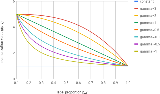
where $\alpha$ , $\beta$ and $\gamma$ are the hyperparameters that allow to generalize several standard functions. For instance with $\alpha=1$ , $\beta=0$ and $\gamma=-1$ , this function weights each example inversely proportional to the proportion of labels. This is equivalent to normalizing by the number of known classes instead of the number of classes. Given a $\gamma$ value and the weight for a given proportion (e.g. $g(0.1)=5$ ), we can find the hyperparameters $\alpha$ and $\beta$ that satisfy these constraints. The hyperparameter $\gamma$ controls the behavior of the normalization with respect to the label proportion. In Figure 2 we show this function for different values of $\gamma$ given the constraint $g(0.1)=5$ . For $\gamma=1$ the normalization is linearly proportional to the label proportion, whereas for $\gamma=-1$ the normalization value is inversely proportional to the label proportion. We analyse the importance of each hyperparameter in Sec.4. This normalization has a similar goal to batch normalization Ioffe2015 which normalizes distributions of layer inputs for each mini-batch.

3.2 Multi-label classification with GNN

To model the interactions between the categories, we use a Graph Neural Network (GNN) Gori2005; Scarselli2009 on top of a ConvNet. We first introduce the GNN and then detail how we use GNN for multi-label classification.

GNN.

For GNNs, the input data is a graph $\mathcal{G}=\{\mathcal{V},\mathcal{E}\}$ where $\mathcal{V}$ (resp. $\mathcal{E}$ ) is the set of nodes (resp. edges) of the graph. For each node $v\in\mathcal{V}$ , we denote the input feature vector $\mathbf{x}_{v}$ and its hidden representation describing the node’s state at time step $t$ by $\mathbf{h}_{v}^{t}$ . We use $\Omega_{v}$ to denote the set of neighboring nodes of $v$ . A node uses information from its neighbors to update its hidden state. The update is decomposed into two steps: message update and hidden state update. The message update step combines messages sent to node $v$ into a single message vector $\mathbf{m}_{v}^{t}$ according to:

\mathbf{m}_{v}^{t}=\mathcal{M}(\{\mathbf{h}_{u}^{t}|u\in\Omega_{v}\})

(3)

where $\mathcal{M}$ is the function to update the message. In the hidden state update step, the hidden states $\mathbf{h}_{v}^{t}$ at each node in the graph are updated based on messages $\mathbf{m}_{v}^{t}$ according to:

\mathbf{h}_{v}^{t+1}=\mathcal{F}(\mathbf{h}_{v}^{t},\mathbf{m}_{v}^{t})

(4)

where $\mathcal{F}$ is the function to update the hidden state. $\mathcal{M}$ and $\mathcal{F}$ are feedforward neural networks that are shared among different time steps. Note that these update functions specify a propagation model of information inside the graph.

GNN for multi-label classification.

For multi-label classification, each node represents one category ( $\mathcal{V}=\{1,\ldots,C\}$ ) and the edges represent the connections between the categories. We use a fully-connected graph to model correlation between all categories. The node hidden states are initialized with the ConvNet output. We now detail the GNN functions used in our model. The algorithm and additional information are given in the supplementary material.

Message update function $\mathcal{M}$ .

We use the following message update function:

\mathbf{m}_{v}^{t}=\frac{1}{|\Omega_{v}|}\sum_{u\in\Omega_{v}}f_{\mathcal{M}}(\mathbf{h}_{u}^{t})

(5)

where $f_{\mathcal{M}}$ is a multi-layer perceptron (MLP). The message is computed by first feeding hidden states to the MLP $f_{\mathcal{M}}$ and then taking the average over the neighborhood.

Hidden state update function $\mathcal{F}$ .

We use the following hidden state update function:

\mathbf{h}_{v}^{t+1}=GRU(\mathbf{h}_{v}^{t},\mathbf{m}_{v}^{t})

(6)

which uses a Gated Recurrent Unit (GRU) Cho2014. The hidden state is updated based on the incoming messages and the previous hidden state.

3.3 Prediction of unknown labels

In this section, we propose a method to predict some missing labels with a curriculum learning strategy Bengio2009. We formulate our problem based on the self-paced model Kumar2010; Jiang2015 and the goal is to optimize the following objective function:

	$\displaystyle\underset{\mathbf{w}\in\mathbb{R}^{d},\mathbf{v}\in\{0,1\}^{N\times C}}{\min}$	$\displaystyle~J(\mathbf{w},\mathbf{v})=\beta\\|\mathbf{w}\\|^{2}+G(\mathbf{v};\theta)$		(7)
		$\displaystyle+\frac{1}{N}\sum_{i=1}^{N}\frac{1}{C}\sum_{c=1}^{C}v_{ic}\ell_{c}(f_{\mathbf{w}}(\mathcal{I}^{(i)}),y_{c}^{(i)})$

where $\ell_{c}$ is the loss for category $c$ and $v_{i}\in\{0,1\}^{C}$ is a vector to represent the selected labels for the i-th sample. $v_{ic}=1$ (resp. $v_{ic}=0$ ) means that the $c$ -th label of the $i$ -th example is selected (resp. unselected). The function $G$ defines a curriculum, parameterized by $\theta$ , which defines the learning scheme. Following Kumar2010, we use an alternating algorithm where $\mathbf{w}$ and $\mathbf{v}$ are alternatively minimized, one at a time while the other is held fixed. The algorithm is shown in Algorithm 1. Initially, the model is learned with only clean partial labels. Then, the algorithm uses the learned model to add progressively new “easy” weak (i.e. noisy) labels in the training set, and then uses the clean and weak labels to continue the training of the model. We analyze different strategies to add new labels:

[a] Score threshold strategy. This strategy uses the classification score (i.e. ConvNet) to estimate the difficulty of a pair category-example. An easy example has a high absolute score whereas a hard example has a score close to 0. We use the learned model on partial labels to predict the missing labels only if the classification score is larger than a threshold $\theta>0$ . When $\mathbf{w}$ is fixed, the optimal $\mathbf{v}$ can be derived by:

\displaystyle v_{ic}=\mathds{1}[x_{c}^{(i)}\geq\theta]+\mathds{1}[x_{c}^{(i)}<-\theta]

(8)

The predicted label is $y_{c}^{(i)}=\sign(x_{c}^{(i)})$ .

[b] Score proportion strategy. This strategy is similar to the strategy [a] but instead of labeling the pair category-example higher than a threshold, we label a fixed proportion $\theta$ of pairs per mini-batch. To find the optimal $\mathbf{v}$ , we sort the examples by decreasing order of absolute score and label only the top- $\theta$ % of the missing labels.

[c] Predict only positive labels. Because of the imbalanced annotations, we only predict positive labels with strategy [a]. When $\mathbf{w}$ is fixed, the optimal $\mathbf{v}$ can be derived by:

\displaystyle v_{ic}=\mathds{1}[x_{c}^{(i)}\geq\theta]

(9)

[d] Ensemble score threshold strategy. This strategy is similar to the strategy [a] but it uses an ensemble of models to estimate the confidence score. We average the classification score of each model to estimate the final confidence score. This strategy allows to be more robust than the strategy [a]. When $\mathbf{w}$ is fixed, the optimal $\mathbf{v}$ can be derived by:

\displaystyle v_{ic}=\mathds{1}[E(\mathcal{I}^{(i)})_{c}\geq\theta]+\mathds{1}[E(\mathcal{I}^{(i)})_{c}<-\theta]

(10)

where $E(\mathcal{I}^{(i)})\in\mathbb{R}^{C}$ is the vector score of an ensemble of models. The predicted label is $y_{c}^{(i)}=\sign(E(\mathcal{I}^{(i)})_{c})$ .

[e] Bayesian uncertainty strategy. Instead of using the classification score as in [a] or [d], we estimate the bayesian uncertainty Kendall2017 of each pair category-example. An easy pair category-example has a small uncertainty. When $\mathbf{w}$ is fixed, the optimal $\mathbf{v}$ can be derived by:

\displaystyle v_{ic}=\mathds{1}[U(\mathcal{I}^{(i)})_{c}\leq\theta]

(11)

where $U(\mathcal{I}^{(i)})$ is the bayesian uncertainty of category $c$ of the $i$ -th example. This strategy is similar to strategy [d] except that it uses the variance of the classification scores instead of the average to estimate the difficulty.

Algorithm 1 Curriculum labeling

0: Training data

\mathcal{D}

1: Initialize

\mathbf{v}

with known labels

2: Initialize

\mathbf{w}

: learn the ConvNet with the partial labels

3: repeat

4: Update

\mathbf{v}

(fixed

\mathbf{w}

): find easy missing labels

5: Update

\mathbf{y}

: predict the label of easy missing labels

6: Update

\mathbf{w}

(fixed

\mathbf{v}

): improve classification model with the clean and easy weak annotations

7: until stopping criteria

4 Experiments

Datasets.

We perform experiments on several standard multi-label datasets: Pascal VOC 2007 Everingham2015, MS COCO Lin2014 and NUS-WIDE Chua2009. For each dataset, we use the standard train/test sets introduced respectively in Everingham2015, Oquab2014, and Gong2014 (see subsection A.2 of supplementary for more details). From these datasets that are fully labeled, we create partially labeled datasets by randomly dropping some labels per image. The proportion of known labels is between 10% (90% of labels missing) and 100% (all labels present). We also perform experiments on the large-scale Open Images dataset Kuznetsova2018 that is partially annotated: $0.9\%$ of the labels are available during training.

Metrics.

To evaluate the performances, we use several metrics: mean Average Precision (MAP) BaezaYates1999, 0-1 exact match, Macro-F1 Yang1999, Micro-F1 Tang2009, per-class precision, per-class recall, overall precision, overall recall. These metrics are standard multi-label classification metrics and are presented in subsection A.3 of supplementary. We mainly show the results for the MAP metric but results for other metrics are shown in supplementary.

Implementation details.

We employ ResNet-WELDON Durand2018 as our classification network. We use a ResNet-101 He2016 pretrained on ImageNet as the backbone architecture, but we show results for other architectures in supplementary. The models are implemented with PyTorch Paszke2017. The hyperparameters of the partial-BCE loss function are $\alpha=-4.45$ , $\beta=5.45$ (i.e. $g(0.1)=5$ ) and $\gamma=1$ . To predict missing labels, we use the bayesian uncertainty strategy with $\theta=0.3$ .

4.1 What is the best strategy to annotate a dataset?

In the first set of experiments, we study three strategies to annotate a multi-label dataset. The goal is to answer the question: what is the best strategy to annotate a dataset with a fixed budget of clean labels? We explore the three following scenarios:

•

Partial labels. This is the strategy used in this paper. In this setting, all the images are used but only a subset of the labels per image are known. The known categories are different for each image.
•

Complete image labels or dense labels. In this scenario, only a subset of the images are labeled, but the labeled images have the annotations for all the categories. This is the standard setting for semi-supervised learning Chapelle2010 except that we do not use a semi-supervised model.
•

Noisy labels. All the categories of all images are labeled but some labels are wrong. This scenario is similar to the webly-supervised learning scenario Mahajan2018 where some labels are wrong.

To have fair comparison between the approaches, we use a BCE loss function for these experiments. The results are shown in Figure 3 for different proportion of clean labels. For each experiment, we use the same number of clean labels. $100\%$ means that all the labels are known during training (standard classification setting) and $10\%$ means that only $10\%$ of the labels are known during training. The 90% of other labels are unknown labels for the partial labels and the complete image labels scenarios and are wrong labels for the noisy labels scenario. Similar to Sun2017, we observe that the performance increases logarithmically based on proportion of labels. From this first experiment, we can draw the following conclusions: (1) Given a fixed number of clean labels, we observe that learning with partial labels is better than learning with a subset of dense annotations. The improvement increases when the label proportion decreases. A reason is that the model trained in the partial labels strategy “sees” more images during training and therefore has a better generalization performance. (2) It is better to learn with a small subset of clean labels than a lot of labels with some incorrect labels. Both partial labels and complete image labels scenarios are better than the noisy label scenario. For instance on MS COCO, we observe that learning with only 20% of clean partial labels is better than learning with 80% of clean labels and 20% of wrong labels.

Noisy web labels.

Another strategy to generate a noisy dataset from a multi-label dataset is to use only one positive label for each image. This is a standard assumption made when collecting data from the web Li2017c i.e. the only category present in the image is the category of the query. From the clean MS COCO dataset, we generate a noisy dataset (named noisy+) by keeping only one positive label per image. If the image has more than one positive label, we randomly select one positive label among the positive labels and switch the other positive labels to negative labels. The results are reported in Table 1 for three scenarios: clean (all the training labels are known and clean), 10% of partial labels and noisy+ scenario. We also show the percentage of clean and noisy labels for each experiment. The noisy+ approach generates a small proportion of noisy labels (2.4%) that drops the performance by about 7pt with respect to the clean baseline. We observe that a model trained with only 10% of clean labels is slightly better than the model trained with the noisy labels. This experiment shows that the standard assumption made in most of the webly-supervised datasets is not good for complex scenes / multi-label images because it generates noisy labels that significantly decrease generalization.

model	clean	partial 10%	noisy+
clean / noisy labels	100 / 0	10 / 0	97.6 / 2.4
MAP (%)	79.22	72.15	71.60

Table 1: Comparison with a webly-supervised strategy (noisy+) on MS COCO. Clean (resp. noisy) means the percentage of clean (resp. noisy) labels in the training set.

Relabeling	MAP	0-1	Macro-F1	Micro-F1	label prop.	TP	TN	GNN
2 steps (no curriculum)	-1.49	6.42	2.32	1.99	100	82.78	96.40	✓
[a] Score threshold $\theta=2$	0.34	11.15	4.33	4.26	95.29	85.00	98.50	✓
[b] Score proportion $\theta=80\%$	0.17	8.40	3.70	3.25	96.24	84.40	98.10	✓
[c] Postitive only - score $\theta=5$	0.31	-4.58	-1.92	-2.23	12.01	79.07	-	✓
[d] Ensemble score $\theta=2$	0.23	11.31	4.16	4.33	95.33	84.80	98.53	✓
[e] Bayesian uncertainty $\theta=0.3$	0.34	10.15	4.37	3.72	77.91	61.15	99.24
[e] Bayesian uncertainty $\theta=0.1$	0.36	2.71	1.91	1.22	19.45	38.15	99.97	✓
[e] Bayesian uncertainty $\theta=0.2$	0.30	10.76	4.87	4.66	57.03	62.03	99.65	✓
[e] Bayesian uncertainty $\theta=0.3$	0.59	12.07	5.11	4.95	79.74	68.96	99.23	✓
[e] Bayesian uncertainty $\theta=0.4$	0.43	10.99	4.88	4.46	90.51	70.77	98.57	✓
[e] Bayesian uncertainty $\theta=0.5$	0.45	10.08	3.93	3.78	94.79	74.73	98.00	✓

Table 2: Analysis of the labeling strategy of missing labels on Pascal VOC 2007 val set. For each metric, we report the relative scores with respect to a model that does not label missing labels. TP (resp. TN) means true positive (resp. true negative) rate. For the strategy [c], we report the label accuracy instead of the TP rate.

4.2 Learning with partial labels

In this section, we compare the standard BCE and the partial-BCE and analyze the importance of the GNN.

BCE vs partial-BCE.

The Figure 3 shows the MAP results for different proportion of known labels on three datasets. For all the datasets, we observe that using the partial-BCE significantly improves the performance: the lower the label proportion, the better the improvement. We observe the same behavior for the other metrics (subsection A.6 of supplementary). In Table 3, we show results on the Open Images dataset and we observe that the partial-BCE is 4 pt better than the standard BCE. These experiments show that our loss learns better than the BCE because it exploits the label proportion information during training. It allows to learn efficiently while keeping the same training setting as with all annotations.

	BCE	partial-BCE	GNN + partial-BCE
MAP (%)	79.01	83.05	83.36

Table 3: MAP results on Open Images.

GNN.

We now analyze the improvements of the GNN to learn relationships between the categories. We show the results on MS COCO in Figure 4. We observe that for each label proportion, using the GNN improves the performance. Open Images experiments (Table 3) show that GNN improves the performance even when the label proportion is small. This experiment shows that modeling the correlation between categories is important even in case of partial labels. However, we also note that a ConvNet implicitly learns some correlation between the categories because some learned representations are shared by all categories.

BCE	fine-tuning	partial-BCE	GNN	relabeling	MAP	0-1 exact match	Macro-F1	Micro-F1
✓					66.21	17.53	62.74	67.33
✓	✓				72.15	22.04	65.82	70.09
	✓	✓			75.31	24.51	67.94	71.18
	✓	✓	✓		75.82	25.14	68.40	71.37
	✓	✓		✓	75.71	30.52	70.13	73.87
	✓	✓	✓	✓	76.40	32.12	70.73	74.37

Table 4: Ablation study on MS COCO with 10% of known labels.

4.3 What is the best strategy to predict missing labels?

In this section, we analyze the labeling strategies introduced in subsection 3.3 to predict missing labels. Before training epochs 10 and 15, we use the learned classifier to predict some missing labels. We report the results for different metrics on Pascal VOC 2007 validation set with 10% of labels in Table 2. We also report the final proportion of labels, the true postive (TP) and true negative (TN) rates for predicted labels. Additional results are shown in subsection A.9 of supplementary.

First, we show the results of a 2 steps strategy that predicts all missing labels in one time. Overall, we observe that this strategy is worse than curriculum-based strategies ([a-e]). In particular, the 2 steps strategy decreases the MAP score. These results show that predicting all missing labels at once introduced too much label noise, decreasing generalization performance. Among the curriculum-based strategies, we observe that the threshold strategy [a] is better than the proportion strategy [b]. We also note that using a model ensemble [d] does not significantly improve the performance with respect to a single model [a]. Predicting only positive labels [c] is a poor strategy. The bayesian uncertainty strategy [e] is the best strategy. In particular, we observe that the GNN is important for this strategy because it decreases the label uncertainty and allows the model to be robust to the hyperparameter $\theta$ .

4.4 Method analysis

In this section, we analyze the hyperparameters of the partial-BCE and perform an ablation study on MS COCO.

Partial-BCE analysis.

To analyze the partial-BCE, we use only the training set. The model is trained on about 78k images and evaluated on the remaining 5k images. We first analyse how to choose the value of the normalization function given a label proportion of 10% i.e. $g(0.1)$ (it is possible to choose another label proportion). The results are shown in Figure 5. Note that for $g(0.1)=1$ , the partial-BCE is equivalent to the BCE and the loss is normalized by the number of categories. We observe that the normalization value $g(0.1)=1$ gives the worst results. The best score is obtained for a normalization value around 20 but the performance is similar for $g(0.1)\in[3,50]$ . Using a large value drops the performance. This experiment shows that the proposed normalization function is important and robust. These results are independent of the network architectures (subsection A.7 of supplementary).

Given the constraints $g(0.1)=5$ and $g(1)=1$ , we analyze the impact of the hyperparameter $\gamma$ . This hyperparameter controls the behavior of the normalization with respect to the label proportion. Using a high value ( $\gamma=3$ ) is better than a low value ( $\gamma=-1$ ) for large label proportions but is slighty worse for small label proportions. We observe that using a normalization that is proportional to the number of known labels ( $\gamma=1$ ) works better than using a normalization that is inversely proportional to the number of known labels ( $\gamma=-1$ ).

Ablation study.

Finally to analyze the importance of each contribution, we perform an ablation study on MS COCO for a label proportion of 10% in Table 4. We first observe that fine-tuning is important. It validates the importance of building end-to-end trainable models to learn with missing labels. The partial-BCE loss function increases the performance against each metric because it exploits the label proportion information during training. We show that using GNN or relabeling improves performance. In particular, the relabeling stage significantly increases the 0-1 exact match score (+5pt) and the Micro-F1 score (+2.5pt). Finally, we observe that our contributions are complementary.

5 Conclusion

In this paper, we present a scalable approach to end-to-end learn a multi-label classifier with partial labels. Our experiments show that our loss function significantly improves performance. We show that our curriculum learning model using bayesian uncertainty is an accurate strategy to label missing labels. In the future work, one could combine several datasets whith shared categories to learn with more training data.

References

(1) R. A. Baeza-Yates and B. Ribeiro-Neto. Modern Information Retrieval. 1999.
(2) Y. Bengio, J. Louradour, R. Collobert, and J. Weston. Curriculum learning. In International Conference on Machine Learning (ICML), 2009.
(3) S. S. Bucak, R. Jin, and A. K. Jain. Multi-label learning with incomplete class assignments. In IEEE Conference on Computer Vision and Pattern Recognition (CVPR), 2011.
(4) R. S. Cabral, F. Torre, J. P. Costeira, and A. Bernardino. Matrix Completion for Multi-label Image Classification. In Advances in Neural Information Processing Systems (NIPS), 2011.
(5) A. Carlson, J. Betteridge, B. Kisiel, B. Settles, E. R. H. Jr., and T. M. Mitchell. Toward an Architecture for Never-Ending Language Learning. In Conference on Artificial Intelligence (AAAI), 2010.
(6) O. Chapelle, B. Schlkopf, and A. Zien. Semi-Supervised Learning. 2010.
(7) X. Chen, A. Shrivastava, and A. Gupta. Neil: Extracting visual knowledge from web data. In IEEE International Conference on Computer Vision (ICCV), 2013.
(8) X. Chen, A. Shrivastava, and A. Gupta. Enriching visual knowledge bases via object discovery and segmentation. In IEEE Conference on Computer Vision and Pattern Recognition (CVPR), 2014.
(9) K. Cho, B. van Merrienboer, D. Bahdanau, and Y. Bengio. On the properties of neural machine translation: Encoder-decoder approaches. In Eighth Workshop on Syntax, Semantics and Structure in Statistical Translation (SSST-8), 2014.
(10) H.-M. Chu, C.-K. Yeh, and Y.-C. Frank Wang. Deep Generative Models for Weakly-Supervised Multi-Label Classification. In European Conference on Computer Vision (ECCV), 2018.
(11) T.-S. Chua, J. Tang, R. Hong, H. Li, Z. Luo, and Y. Zheng. NUS-WIDE: A Real-world Web Image Database from National University of Singapore. In ACM International Conference on Image and Video Retrieval (CIVR), 2009.
(12) T. Cour, B. Sapp, and B. Taskar. Learning from Partial Labels. Journal of Machine Learning Research (JMLR), 2011.
(13) J. Deng, O. Russakovsky, J. Krause, M. S. Bernstein, A. Berg, and L. Fei-Fei. Scalable Multi-label Annotation. In Proceedings of the SIGCHI Conference on Human Factors in Computing Systems, 2014.
(14) T. Durand, T. Mordan, N. Thome, and M. Cord. WILDCAT: Weakly Supervised Learning of Deep ConvNets for Image Classification, Pointwise Localization and Segmentation. In IEEE Conference on Computer Vision and Pattern Recognition (CVPR), 2017.
(15) T. Durand, N. Thome, and M. Cord. WELDON: Weakly Supervised Learning of Deep Convolutional Neural Networks. In IEEE Conference on Computer Vision and Pattern Recognition (CVPR), 2016.
(16) T. Durand, N. Thome, and M. Cord. Exploiting Negative Evidence for Deep Latent Structured Models. In IEEE Transactions on Pattern Analysis and Machine Intelligence (TPAMI), 2018.
(17) M. Everingham, S. M. A. Eslami, L. Van Gool, C. K. I. Williams, J. Winn, and A. Zisserman. The Pascal Visual Object Classes Challenge: A Retrospective. International Journal of Computer Vision (IJCV), 2015.
(18) Y. Gong, Y. Jia, T. Leung, A. Toshev, and S. Ioffe. Deep Convolutional Ranking for Multilabel Image Annotation. In International Conference on Learning Representations (ICLR), 2014.
(19) M. Gori, G. Monfardini, and F. Scarselli. A new model for learning in graph domains. In IEEE International Joint Conference on Neural Networks (IJCNN), 2005.
(20) S. Guo, W. Huang, H. Zhang, C. Zhuang, D. Dong, M. R. Scott, and D. Huang. CurriculumNet: Weakly Supervised Learning from Large-Scale Web Images. In European Conference on Computer Vision (ECCV), 2018.
(21) K. He, X. Zhang, S. Ren, and J. Sun. Deep residual learning for image recognition. In IEEE Conference on Computer Vision and Pattern Recognition (CVPR), 2016.
(22) S. Ioffe and C. Szegedy. Batch Normalization: Accelerating Deep Network Training by Reducing Internal Covariate Shift. In International Conference on Machine Learning (ICML), 2015.
(23) F. V. Jensen and T. D. Nielsen. Bayesian Networks and Decision Graphs. 2007.
(24) L. Jiang, D. Meng, Q. Zhao, S. Shan, and A. G. Hauptmann. Self-Paced Curriculum Learning. In Conference on Artificial Intelligence (AAAI), 2015.
(25) L. Jiang, Z. Zhou, T. Leung, L.-J. Li, and L. Fei-Fei. MentorNet: Learning Data-Driven Curriculum for Very Deep Neural Networks on Corrupted Labels. In International Conference on Machine Learning (ICML), 2018.
(26) A. Joulin, L. van der Maaten, A. Jabri, and N. Vasilache. Learning visual features from large weakly supervised data. In European Conference on Computer Vision (ECCV), 2016.
(27) A. Kapoor, R. Viswanathan, and P. Jain. Multilabel classification using bayesian compressed sensing. In Advances in Neural Information Processing Systems (NIPS), 2012.
(28) A. Kendall and Y. Gal. What uncertainties do we need in bayesian deep learning for computer vision? In Advances in Neural Information Processing Systems (NIPS), 2017.
(29) D. P. Kingma and M. Welling. Auto-Encoding Variational Bayes. In International Conference on Learning Representations (ICLR), 2014.
(30) S. Kornblith, J. Shlens, and Q. V. Le. Do Better ImageNet Models Transfer Better? 2018.
(31) M. P. Kumar, B. Packer, and D. Koller. Self-paced learning for latent variable models. In Advances in Neural Information Processing Systems (NIPS), 2010.
(32) A. Kuznetsova, H. Rom, N. Alldrin, J. Uijlings, I. Krasin, J. Pont-Tuset, S. Kamali, S. Popov, M. Malloci, T. Duerig, and V. Ferrari. The Open Images Dataset V4: Unified image classification, object detection, and visual relationship detection at scale. 2018.
(33) L. J. Li, G. Wang, and L. Fei-Fei. OPTIMOL: automatic Online Picture collecTion via Incremental MOdel Learning. In IEEE Conference on Computer Vision and Pattern Recognition (CVPR), 2007.
(34) W. Li, L. Wang, W. Li, E. Agustsson, J. Berent, A. Gupta, R. Sukthankar, and L. Van Gool. WebVision Challenge: Visual Learning and Understanding With Web Data. In arXiv 1705.05640, 2017.
(35) Y. Li, Y. Song, and J. Luo. Improving Pairwise Ranking for Multi-label Image Classification. In IEEE Conference on Computer Vision and Pattern Recognition (CVPR), 2017.
(36) T.-Y. Lin, M. Maire, S. Belongie, L. Bourdev, R. Girshick, J. Hays, P. Perona, D. Ramanan, C. L. Zitnick, and P. Dollár. Microsoft COCO: Common Objects in Context. 2014.
(37) C. Liu, B. Zoph, J. Shlens, W. Hua, L.-J. Li, L. Fei-Fei, A. Yuille, J. Huang, and K. Murphy. Progressive Neural Architecture Search. In European Conference on Computer Vision (ECCV), 2018.
(38) D. Mahajan, R. Girshick, V. Ramanathan, K. He, M. Paluri, Y. Li, A. Bharambe, and L. van der Maaten. Exploring the Limits of Weakly Supervised Pretraining. In European Conference on Computer Vision (ECCV), 2018.
(39) Minmin Chen and Alice Zheng and Kilian Weinberger. Fast image tagging. In International Conference on Machine Learning (ICML), 2013.
(40) T. Mitchell, W. Cohen, E. Hruschka, P. Talukdar, J. Betteridge, A. Carlson, B. Dalvi, M. Gardner, B. Kisiel, J. Krishnamurthy, N. Lao, K. Mazaitis, T. Mohamed, N. Nakashole, E. Platanios, A. Ritter, M. Samadi, B. Settles, R. Wang, D. Wijaya, A. Gupta, X. Chen, A. Saparov, M. Greaves, and J. Welling. Never-Ending Learning. In Conference on Artificial Intelligence (AAAI), 2015.
(41) M. Oquab, L. Bottou, I. Laptev, and J. Sivic. Learning and Transferring Mid-Level Image Representations using Convolutional Neural Networks. In IEEE Conference on Computer Vision and Pattern Recognition (CVPR), 2014.
(42) M. Oquab, L. Bottou, I. Laptev, and J. Sivic. Is Object Localization for Free? - Weakly-Supervised Learning With Convolutional Neural Networks. In IEEE Conference on Computer Vision and Pattern Recognition (CVPR), 2015.
(43) A. Paszke, S. Gross, S. Chintala, G. Chanan, E. Yang, Z. DeVito, Z. Lin, A. Desmaison, L. Antiga, and A. Lerer. Automatic differentiation in pytorch. In Advances in Neural Information Processing Systems (NIPS), 2017.
(44) H. Pham, M. Y. Guan, B. Zoph, Q. V. Le, and J. Dean. Faster Discovery of Neural Architectures by Searching for Paths in a Large Model. In International Conference on Learning Representations (ICLR), 2018.
(45) X. Qi, R. Liao, J. Jia, S. Fidler, and R. Urtasun. 3D Graph Neural Networks for RGBD Semantic Segmentation. In IEEE International Conference on Computer Vision (ICCV), 2017.
(46) C. J. V. Rijsbergen. Information Retrieval. 1979.
(47) O. Russakovsky, J. Deng, H. Su, J. Krause, S. Satheesh, S. Ma, Z. Huang, A. Karpathy, A. Khosla, M. Bernstein, A. C. Berg, and L. Fei-Fei. ImageNet large scale visual recognition challenge. International Journal of Computer Vision (IJCV), 2015.
(48) F. Scarselli, M. Gori, A. C. Tsoi, M. Hagenbuchner, and G. Monfardini. The graph neural network model. IEEE Transactions on Neural Networks, 2009.
(49) P. Stock and M. Cisse. ConvNets and ImageNet Beyond Accuracy: Understanding Mistakes and Uncovering Biases. In European Conference on Computer Vision (ECCV), 2018.
(50) C. Sun, M. Paluri, R. Collobert, R. Nevatia, and L. Bourdev. ProNet: Learning to Propose Object-Specific Boxes for Cascaded Neural Networks. In IEEE Conference on Computer Vision and Pattern Recognition (CVPR), 2016.
(51) C. Sun, A. Shrivastava, S. Singh, and A. Gupta. Revisiting Unreasonable Effectiveness of Data in Deep Learning Era. In IEEE International Conference on Computer Vision (ICCV), 2017.
(52) Y.-Y. Sun, Y. Zhang, and Z.-H. Zhou. Multi-label Learning with Weak Label. In Conference on Artificial Intelligence (AAAI), 2010.
(53) C. Szegedy, S. Ioffe, V. Vanhoucke, and A. Alemi. Inception-v4, inception-resnet and the impact of residual connections on learning. In Conference on Artificial Intelligence (AAAI), 2017.
(54) L. Tang, S. Rajan, and V. K. Narayanan. Large scale multi-label classification via metalabeler. In WWW, 2009.
(55) G. Tsoumakas and I. Katakis. Multi-label classification: An overview. International Journal of Data Warehousing and Mining (IJDWM), 2007.
(56) A. Vahdat. Toward robustness against label noise in training deep discriminative neural networks. In Advances in Neural Information Processing Systems (NIPS), 2017.
(57) D. Vasisht, A. Damianou, M. Varma, and A. Kapoor. Active Learning for Sparse Bayesian Multilabel Classification. In ACM SIGKDD International Conference on Knowledge Discovery and Data Mining, 2014.
(58) Q. Wang, B. Shen, S. Wang, L. Li, and L. Si. Binary Codes Embedding for Fast Image Tagging with Incomplete Labels. In European Conference on Computer Vision (ECCV), 2014.
(59) B. Wu, S. Lyu, and B. Ghanem. ML-MG: Multi-Label Learning With Missing Labels Using a Mixed Graph. In IEEE International Conference on Computer Vision (ICCV), 2015.
(60) S. Xie, R. Girshick, P. Dollár, Z. Tu, and K. He. Aggregated Residual Transformations for Deep Neural Networks. In IEEE Conference on Computer Vision and Pattern Recognition (CVPR), 2017.
(61) M. Xu, R. Jin, and Z.-H. Zhou. Speedup Matrix Completion with Side Information: Application to Multi-Label Learning. In Advances in Neural Information Processing Systems (NIPS), 2013.
(62) H. Yang, J. T. Zhou, and J. Cai. Improving Multi-label Learning with Missing Labels by Structured Semantic Correlations. In European Conference on Computer Vision (ECCV), 2016.
(63) Y. Yang. An evaluation of statistical approaches to text categorization. 1999.
(64) H.-F. Yu, P. Jain, P. Kar, and I. S. Dhillon. Large-scale Multi-label Learning with Missing Labels. In International Conference on Machine Learning (ICML), 2014.
(65) C. Zhang, S. Bengio, M. Hardt, B. Recht, and O. Vinyals. Understanding deep learning requires rethinking generalization. In International Conference on Learning Representations (ICLR), 2017.
(66) B. Zhou, A. Khosla, A. Lapedriza, A. Oliva, and A. Torralba. Learning Deep Features for Discriminative Localization. In IEEE Conference on Computer Vision and Pattern Recognition (CVPR), 2016.
(67) B. Zoph, V. Vasudevan, J. Shlens, and Q. V. Le. Learning transferable architectures for scalable image recognition. In IEEE Conference on Computer Vision and Pattern Recognition (CVPR), 2018.

Appendix A Supplementary

A.1 Multi-label classification with GNN

In this section, we give additional information about the Graph Neural Networks (GNN) used in our work. We first show the algorithm used to predict the classification scores with a GNN in Algorithm 2. The input $\mathbf{x}\in\mathbb{R}^{C}$ of the GNN is the ConvNet output, where $C$ is the number of categories.

The $f_{\mathcal{M}}$ function in the message update function $\mathcal{M}$ is a fully connected layer followed by a ReLU. Because the graph is fully-connected, the message update function $\mathcal{M}$ averages on all the nodes of the graph excepts the current node $v$ i.e. $\Omega_{v}=\mathcal{V}\setminus\{v\}$ . Similarly to Qi2017, the final prediction uses both first and last hidden states. We observe that using both first and last hidden states is better than using only the last hidden state. According to Qi2017, we use $T=3$ iterations in our experiments.

Algorithm 2 Graph Neural Network (GNN)

0: ConvNet output

\mathbf{x}

1: Initialize the hidden state of each node

v\in\mathcal{V}

with the output of the ConvNet.

\mathbf{h}_{v}^{0}=[0,\ldots,0,x_{v},0,\ldots,0]\qquad\forall v\in\mathcal{V}

(12)

2: for t = 0 to T-1 do

3: Update message of each node

v\in\mathcal{V}

based on the hidden states

\mathbf{m}_{v}^{t}=\mathcal{M}(\{\mathbf{h}_{u}^{t}|u\in\Omega_{v}\})=\frac{1}{|\Omega_{v}|}\sum_{u\in\Omega_{v}}f_{\mathcal{M}}(\mathbf{h}_{u}^{t})

(13)

4: Update hidden state of each node

v\in\mathcal{V}

based on the messages

\mathbf{h}_{v}^{t+1}=\mathcal{F}(\mathbf{h}_{v}^{t},\mathbf{m}_{v}^{t})=GRU(\mathbf{h}_{v}^{t},\mathbf{m}_{v}^{t})

(14)

5: end for

6: Compute the output based on the first and last hidden states

\bar{\mathbf{y}}=s(\mathbf{h}_{v}^{0},\mathbf{h}_{v}^{T})=\mathbf{h}_{v}^{0}+\mathbf{h}_{v}^{T}

(15)

\bar{\mathbf{y}}

A.2 Experimental details

Datasets.

We perform experiments on large publicly available multi-label datasets: Pascal VOC 2007 Everingham2015, MS COCO Lin2014 and NUS-WIDE Chua2009. Pascal VOC 2007 dataset contains 5k/5k trainval/test images of 20 objects categories. MS COCO dataset contains 123k images of 80 objects categories. We use the 2014 data split with 83k train images and 41k val images. NUS-WIDE dataset contains 269,648 images downloaded from Flickr that have been manually annotated with 81 visual concepts. We follow the experimental protocol in Gong2014 and use 150k randomly sampled images for training and the rest for testing. The results on NUS-WIDE cannot be directly comparable with the other works because the number of total images is different (209,347 in Gong2014, 200,261 in Li2017b). The main reason is that some provided URLs are invalid or some images have been deleted from Flickr. For our experiments, we collected 216,450 images.

We also performs experiments on the largest publicly available multi-label dataset: Open Images Kuznetsova2018. This dataset is partially annotated with human labels and machine generated labels. For our experiments, we use only human labels on the 600 boxable classes. On the training set, only $0.9\%$ of the labels are available.

Implementation details.

The hyperparameters of the WELDON pooling function are $k^{+}=k^{-}=0.1$ . The models are implemented with PyTorch Paszke2017 and are trained with SGD during 20 epochs with a batch size of 16. The initial learning rate is $0.01$ and it is divide by 10 after 10 epochs. During training, we only use random horizontal flip as data augmentation. Each image is resized to $448\times 448$ with 3 color channels. On Open Images dataset, unlike Kuznetsova2018 we do not train from scratch the network. We use a similar protocol that on the others datasets: we fine-tune a model pre-train on ImageNet but stop the training when the validation performance does not increase. Because the training set has 1.7M images, the model converge in less than 5 epochs.

A.3 Multi-label metrics

In this section, we introduce the metrics used to evaluate the performances on multi-label datasets. We note $\mathbf{y}^{(i)}=[y^{(i)}_{1},\ldots,y^{(i)}_{C}]\in\mathcal{Y}\subseteq\{-1,0,1\}^{C}$ the ground truth label vector and $\hat{\mathbf{y}}^{(i)}=[\hat{y}^{(i)}_{1},\ldots,\hat{y}^{(i)}_{C}]\in\{-1,1\}^{C}$ the predicted label vector of the $i$ -th example.

Zero-one exact match accuracy (0-1).

This metric considers a prediction correct only if all the labels are correctly predicted:

\displaystyle m_{0/1}(\mathcal{D})=\frac{1}{N}\sum_{i=1}^{N}\mathds{1}[\mathbf{y}^{(i)}=\hat{\mathbf{y}}^{(i)}]

(16)

where $\mathds{1}[.]$ is an indicator function.

Per-class precision/recall (PC-P/R).

	$\displaystyle m_{PC-P}(\mathcal{D})$	$\displaystyle=\frac{1}{C}\sum_{c=1}^{C}\frac{N_{c}^{correct}}{N_{c}^{predict}}$		(17)
	$\displaystyle m_{PC-R}(\mathcal{D})$	$\displaystyle=\frac{1}{C}\sum_{c=1}^{C}\frac{N_{c}^{correct}}{N_{c}^{gt}}$		(18)

where $N_{c}^{correct}$ is the number of correctly predicted images for the $c$ -th label, $N_{c}^{predict}$ is the number of predicted images, $N_{c}^{gt}$ is the number of ground-truth images. Note that the per-class measures treat all classes equal regardless of their sample size, so one can obtain a high performance by focusing on getting rare classes right.

Overall precision/recall (OV-P/R).

Unlike per-class metrics, the overall metrics treat all samples equal regardless of their classes.

	$\displaystyle m_{OV-P}(\mathcal{D})$	$\displaystyle=\frac{\sum_{c=1}^{C}N_{c}^{correct}}{\sum_{c=1}^{C}N_{c}^{predict}}$		(19)
	$\displaystyle m_{OV-R}(\mathcal{D})$	$\displaystyle=\frac{\sum_{c=1}^{C}N_{c}^{correct}}{\sum_{c=1}^{C}N_{c}^{gt}}$		(20)

Macro-F1 (M-F1).

The macro-F1 score Yang1999 is the F1 score Rijsbergen1979 averaged across all categories.

\displaystyle m_{MF1}(\mathcal{D})

\displaystyle=\frac{1}{C}\sum_{c=1}^{C}F_{1}^{c}

(21)

Given a category $c$ , the F1 measure, defined as the harmonic mean of precision and recall, is computed as follows:

\displaystyle F_{1}^{c}=\frac{2P^{c}R^{c}}{P^{c}+R^{c}}

(22)

where the precision ( $P^{c}$ ) and the recall ( $R^{c}$ ) are calculated as follows:

	$\displaystyle P^{c}=\frac{\sum_{i=1}^{N}\mathds{1}[y_{c}^{(i)}=\hat{y}_{c}^{(i)}]}{\sum_{i=1}^{N}\hat{y}_{c}^{(i)}}$		(23)
	$\displaystyle R^{c}=\frac{\sum_{i=1}^{N}\mathds{1}[y_{c}^{(i)}=\hat{y}_{c}^{(i)}]}{\sum_{i=1}^{N}y_{c}^{(i)}}$		(24)

and $y_{c}^{(i)}\in\{0,1\}$

Micro-F1 (m-F1).

The micro-F1 score Tang2009 is computed using the equation of $F_{1}^{c}$ and considering the predictions as a whole

\displaystyle m_{mF1}(\mathcal{D})

\displaystyle=\frac{2\sum_{c=1}^{C}\sum_{i=1}^{N}\mathds{1}[y_{c}^{(i)}=\hat{y}_{c}^{(i)}]}{\sum_{c=1}^{C}\sum_{i=1}^{N}y_{c}^{(i)}+\sum_{c=1}^{C}\sum_{i=1}^{N}\hat{y}_{c}^{(i)}}

(25)

According to the definition, macro-F1 is more sensitive to the performance of rare categories while micro-F1 is affected more by the major categories.

A.4 Analysis of the initial set of labels

In this section, we analyse the initial set of labels for the partial label scenario. We report the results for 4 random seeds to generate the initial set of partial labels. The experiments are performed on MS COCO val2014 with a ResNet-101 WELDON. The results are shown in Table 5 and Figure 7 for different label proportions and metrics. For every label proportion and every metric, we observe that the model is robust to the initial set of labels.

metric	label proportion
metric	10%	20%	30%	40%	50%	60%	70%	80%	90%	100%
MAP	$72.20\!\pm\!0.04$	$74.49\!\pm\!0.02$	$75.77\!\pm\!0.02$	$76.57\!\pm\!0.03$	$77.21\!\pm\!0.01$	$77.73\!\pm\!0.01$	$78.16\!\pm\!0.02$	$78.53\!\pm\!0.03$	$78.85\!\pm\!0.02$	$79.14\!\pm\!0.05$
M-F1	$65.84\!\pm\!0.01$	$69.32\!\pm\!0.04$	$70.66\!\pm\!0.02$	$71.37\!\pm\!0.02$	$71.88\!\pm\!0.03$	$72.29\!\pm\!0.04$	$72.61\!\pm\!0.03$	$72.89\!\pm\!0.03$	$73.05\!\pm\!0.06$	$73.24\!\pm\!0.02$
m-F1	$70.13\!\pm\!0.04$	$73.97\!\pm\!0.01$	$75.36\!\pm\!0.01$	$76.07\!\pm\!0.03$	$76.54\!\pm\!0.01$	$76.91\!\pm\!0.02$	$77.17\!\pm\!0.04$	$77.42\!\pm\!0.04$	$77.58\!\pm\!0.05$	$77.75\!\pm\!0.04$
0-1	$22.21\!\pm\!0.12$	$30.44\!\pm\!0.03$	$34.26\!\pm\!0.11$	$36.18\!\pm\!0.07$	$37.44\!\pm\!0.05$	$38.46\!\pm\!0.04$	$39.16\!\pm\!0.07$	$39.83\!\pm\!0.12$	$40.34\!\pm\!0.04$	$40.67\!\pm\!0.02$
PC-P	$59.82\!\pm\!0.05$	$68.45\!\pm\!0.10$	$72.56\!\pm\!0.03$	$74.88\!\pm\!0.11$	$76.45\!\pm\!0.04$	$77.70\!\pm\!0.07$	$78.59\!\pm\!0.05$	$79.28\!\pm\!0.10$	$79.80\!\pm\!0.02$	$80.22\!\pm\!0.05$
PC-R	$74.74\!\pm\!0.04$	$71.14\!\pm\!0.07$	$69.66\!\pm\!0.04$	$68.96\!\pm\!0.06$	$68.64\!\pm\!0.04$	$68.35\!\pm\!0.04$	$68.26\!\pm\!0.07$	$68.23\!\pm\!0.08$	$68.12\!\pm\!0.09$	$68.16\!\pm\!0.04$
OV-P	$62.66\!\pm\!0.09$	$72.36\!\pm\!0.06$	$76.81\!\pm\!0.04$	$79.24\!\pm\!0.10$	$80.75\!\pm\!0.06$	$82.01\!\pm\!0.08$	$82.79\!\pm\!0.14$	$83.44\!\pm\!0.10$	$83.94\!\pm\!0.06$	$84.36\!\pm\!0.04$
OV-R	$79.62\!\pm\!0.04$	$75.66\!\pm\!0.04$	$73.97\!\pm\!0.05$	$73.14\!\pm\!0.04$	$72.74\!\pm\!0.04$	$72.40\!\pm\!0.03$	$72.21\!\pm\!0.04$	$72.14\!\pm\!0.01$	$72.07\!\pm\!0.05$	$72.15\!\pm\!0.06$

Table 5: Analysis of the initial set of labels for the partial label scenario. The results are averaged for 4 seeds on MS COCO val2014.

A.5 Analysis of the labeling strategies

In this section we analysis the labeling strategies for different network architectures. The results are shown in Table 6 and Figure 8 on MS COCO dataset. Overall, the results are very similar. For a given proportion of labels, we observe that the partial labels strategy is better that the complete image labels. The improvement increases when the label proportion decreases. The performance of a model learned with noisy labels drops significantly, even for large proportion of clean labels.

In Figure 9, we also show the results for different metrics. For MAP, Macro-F1 and Micro-F1, we observe a similar behaviour: the partial labels strategy has better performances than the complete image labels strategy. For the 0-1 exact match metric, we observe that the complete image labels strategy has better performances than the complete image labels strategy. For this metric, the predictions of all the categories must be corrected, so it advantages the complete image labels strategy because some training images have all the labels whereas in the partial labels strategy, none of the training images have all labels. For the precision and recall metrics, the behaviours are different for the complete image labels strategy and the partial labels strategy. We note that the complete image labels strategy has a better per-class/overall precision than the partial labels strategy but is has a lower per-class/overall recall than the partial labels strategy.

architecture	labels	label proportion
architecture	labels	10%	20%	30%	40%	50%	60%	70%	80%	90%	100%
ResNet-50	partial	61.26	63.78	65.21	66.22	66.97	67.60	68.16	68.58	69.01	69.33
	dense	54.29	59.67	62.50	64.28	65.60	66.68	67.55	68.26	68.80	69.32
	noisy	-	-	-	-	3.75	39.77	56.82	62.93	66.24	69.33
ResNet-50 WELDON	partial	69.91	72.37	73.74	74.53	75.25	75.77	76.25	76.66	77.02	77.28
	dense	62.16	68.04	71.14	73.01	74.17	75.14	75.83	76.42	76.88	77.28
	noisy	-	-	-	-	3.73	52.99	67.08	72.03	74.69	77.29
ResNet-101 WELDON	partial	72.15	74.49	75.76	76.56	77.22	77.73	78.17	78.53	78.84	79.22
	dense	65.22	71.00	73.80	75.44	76.59	77.44	78.08	78.61	78.90	79.24
	noisy	-	-	-	-	3.63	53.10	69.09	74.06	76.85	79.18
ResNeXt-101 WELDON	partial	75.74	77.80	78.95	79.64	80.22	80.61	80.94	81.24	81.48	81.69
	dense	69.03	74.58	77.13	78.50	79.38	80.15	80.65	81.05	81.40	81.71
	noisy	-	-	-	-	3.63	49.26	70.16	75.22	78.28	81.66

Table 6: Comparison of the labeling strategies for different label proportions and different architectures on MS COCO val2014.

Comparison to noisy+ strategy.

In Table 7, we show results for the noisy+ strategy on Pascal VOC 2007, MS COCO and NUS-WIDE for different metrics. For every dataset, we observe that the noisy+ strategy drops the performances of all the metrics with respect to the model learned with only 10% of clean labels.

dataset	strategy	clean label	noisy label	MAP	0-1	M-F1	m-F1	PC-P	PC-R	OV-P	OV-R
VOC 2007	clean	100	0	93.93	79.16	88.90	91.12	90.72	87.34	93.40	88.95
	noisy+	97.1	2.9	90.94	62.21	78.11	78.62	95.41	68.64	97.20	66.00
	partial 10%	10	0	89.09	47.46	74.55	77.84	63.35	94.16	66.02	94.81
MS COCO	clean	100	0	79.22	40.69	73.26	77.80	80.16	68.21	84.31	72.23
	noisy+	97.6	2.4	71.60	20.28	38.62	33.72	91.76	28.17	97.34	20.39
	partial 10%	10	0	72.15	22.04	65.82	70.09	59.76	74.78	62.56	79.68
NUS-WIDE	clean	100	0	54.88	42.29	51.88	71.15	58.54	49.33	73.83	68.66
	noisy+	98.6	1.4	47.44	36.07	18.83	28.53	59.71	13.95	83.72	17.19
	partial 10%	10	0	51.14	25.98	51.36	65.52	41.80	69.23	53.62	84.19

Table 7: Comparison with a webly-supervised strategy (noisy+) on MS COCO. Clean (resp. noisy) means the percentage of clean (resp. noisy) labels in the training set. Noisy+ is a labeling strategy where there is only one positive label per image.

A.6 Comparison of the loss functions

In this section, we analyse the performances of the BCE and partial-BCE loss functions for different metrics. The results on MS COCO (resp. Pascal VOC 2007) are shown in Figure 11 (resp. Figure 13) and the improvement of the partial-BCE with respect to the BCE is shown in Figure 12 (resp. Figure 14). We observe that the partial-BCE significantly improves the performances for MAP, 0-1 exact match, Macro-F1 and Micro-F1 metrics. We note that the improvement is bigger when the label proportion is lower. The proposed loss also improves the (overall and per-class) recall for both datasets. On Pascal VOC 2007, it also improves the overall and per-class precision. However, we observe that the

We observe that decreasing the proportion of known labels can slightly improves the performances with respect to the model trained with all the annotations. This phenomenon is because of the tuning of the learning rate and the hyperparameter $\gamma$ (Figure 6). Note that the BCE and the partial-BCE have the same results for the label proportion 100% because they are equivalent by definition. In the paper, we used the same training setting (learning rate, weight decay, etc.) as Durand2018 for each model and dataset. In Figure 10, we observe that using a learning rate of 0.02 increases the performance and leads to a monotone increase of the performance with respect to the label proportion, but the optimal learning rate depends on the dataset. It is possible to improve the results by tuning carefully these hyperparameters, but we observe that the partial-BCE is still better than the BCE for a large range of LRs and for small label proportions which is the main focus of the paper.

A.7 Analysis of the loss function

In this section, we analyze the hyperparameter of the loss function for several network architectures. The models are trained on the train2014 set minus 5000 images that are used as validation set to evaluate the performances. The Figure 15 shows the results on MS COCO. We observe a similar behavior for all the architectures. Overall, using a normalization value $g(0.1)$ between 3 and 50 significantly improves the performances with respect to the normalization by the number of categories ( $g(0.1)=1$ ). The loss is robust to the value of this hyperparmeter.

A.8 Comparison to existing model for missing labels

As pointed out in the related work section, most of the existing models to learn with missing labels are not scalable and do not allow experiments on large-scale dataset like MS COCO and NUS-WIDE. We compare our model with the APG-Graph model Yang2016 that models structured semantic correlations between images on the Pascal VOC 2007 dataset. Unlike our method, the APG-Graph model does not allow to fine-tune the ConvNet.

A.9 What is the best strategy to predict missing labels?

This section extends the section 4.3 in the paper. First, to compute the Bayesian uncertainty, we use the setting used in the original paper Kendall2017. The results for different strategies and hyperparameters are shown in Table 8. G defines how the examples are selected during training. In the paper, we only explain how to find the solution with respect to $\mathbf{v}$ . G depends on the strategy and is defined as:

\displaystyle G(\mathbf{v};\theta)=-\sum_{i=1}^{N}\sum_{c=1}^{C}v_{ic}\log\left(\frac{1}{1+e^{-\theta}}\right)

for strategy [a].

For strategy [a] and [d], we observe that using a small threshold is better than a large threshold. On the contrary, for strategy [c] we observe that using a large threshold is better than a small threshold, but the results are worse than strategy [a]. For strategy [b], labeling a large proportion of labels per mini-batch is better than labeling a small proportion of labels. For strategy [e], we note that using a GNN improves the performances of the model and the model is more robust to the threshold hyperparameter $\theta$ .

Relabeling	MAP	0-1	Macro-F1	Micro-F1	label prop.	TP	TN	GNN
2 steps (no curriculum)	-1.49	6.42	2.32	1.99	100	82.78	96.40	✓
[a] Score threshold $\theta=1$	0.00	11.31	3.71	4.25	97.87	82.47	97.84	✓
[a] Score threshold $\theta=2$	0.34	11.15	4.33	4.26	95.29	85.00	98.50	✓
[a] Score threshold $\theta=5$	0.31	5.02	2.60	1.83	70.98	96.56	99.44	✓
[b] Score proportion $\theta=0.1$	0.45	-1.20	-0.28	-0.68	26.70	99.28	99.19	✓
[b] Score proportion $\theta=0.2$	0.36	0.20	0.70	0.10	42.09	98.35	99.33	✓
[b] Score proportion $\theta=0.3$	0.28	0.91	1.09	0.37	55.63	97.82	99.38	✓
[b] Score proportion $\theta=0.4$	0.55	2.95	2.33	1.28	67.41	96.87	99.38	✓
[b] Score proportion $\theta=0.5$	0.22	4.02	2.76	1.74	77.40	95.52	99.30	✓
[b] Score proportion $\theta=0.6$	0.41	6.17	3.63	2.52	85.37	93.16	99.15	✓
[b] Score proportion $\theta=0.7$	0.35	7.49	3.83	3.07	91.69	89.40	98.81	✓
[b] Score proportion $\theta=0.8$	0.17	8.40	3.70	3.25	96.24	84.40	98.10	✓
[c] Postitive only - score $\theta=1$	-1.61	-31.75	-18.07	-18.92	16.79	36.42	-	✓
[c] Postitive only - score $\theta=2$	-0.80	-21.31	-10.93	-12.08	14.71	47.94	-	✓
[c] Postitive only - score $\theta=5$	0.31	-4.58	-1.92	-2.23	12.01	79.07	-	✓
[d] Ensemble score $\theta=1$	-0.31	10.16	3.61	3.94	97.84	82.12	97.76	✓
[d] Ensemble score $\theta=2$	0.23	11.31	4.16	4.33	95.33	84.80	98.53	✓
[d] Ensemble score $\theta=5$	0.27	3.78	2.38	1.53	70.77	96.56	99.44	✓
[e] Bayesian uncertainty $\theta=0.1$	0.26	1.84	1.36	0.64	22.63	25.71	99.98
[e] Bayesian uncertainty $\theta=0.2$	0.29	8.49	4.05	3.66	60.32	48.39	99.82
[e] Bayesian uncertainty $\theta=0.3$	0.34	10.15	4.37	3.72	77.91	61.15	99.24
[e] Bayesian uncertainty $\theta=0.4$	0.30	9.05	4.17	3.37	87.80	68.56	98.70
[e] Bayesian uncertainty $\theta=0.5$	0.26	8.32	3.83	3.05	92.90	70.96	98.04
[e] Bayesian uncertainty $\theta=0.1$	0.36	2.71	1.91	1.22	19.45	38.15	99.97	✓
[e] Bayesian uncertainty $\theta=0.2$	0.30	10.76	4.87	4.66	57.03	62.03	99.65	✓
[e] Bayesian uncertainty $\theta=0.3$	0.59	12.07	5.11	4.95	79.74	68.96	99.23	✓
[e] Bayesian uncertainty $\theta=0.4$	0.43	10.99	4.88	4.46	90.51	70.77	98.57	✓
[e] Bayesian uncertainty $\theta=0.5$	0.45	10.08	3.93	3.78	94.79	74.73	98.00	✓

Table 8: Analysis of the labeling strategy of missing labels on Pascal VOC 2007 val set. For each metric, we report the relative scores with respect to a model that does not label missing labels. TP (resp. TN) means true positive (resp. true negative). Label proportion is the proportion of training labels (clean + weak labels) used at the end of the training. For the strategy labeling only positive labels, we report the label accuracy instead of the TP rate.

A.10 Final results

In Figure 17, we show the results of our final model that uses the partial-BCE loss, the GNN and the labeling of missing labels. We compare our model to two baselines: (a) a model trained with the standard BCE where the data are labeled with the partial labels strategy (blue) and (b) a model trained with the standard BCE where the data are labeled with the complete image labels strategy (red). We observe that our model has better performances than the two baselines for most of the metrics. In particular, our final model has significantly better 0-1 exact match performance than the baseline (b), whereas the baseline with partial labels (a) has lower performance than the baseline (b). We note that the overall precision of our model is worse than the baseline (b), but the overall recall of our model is largely better than the baseline (b).

Learning a Deep ConvNet for Multi-label Classification with Partial Labels

Abstract

1 Introduction

2 Related Work

Learning with partial / missing labels.

Curriculum Learning / Never-Ending Learning.

3 Learning with Partial Labels

Notation.

3.1 Binary cross-entropy for partial labels

Normalization function gg

3.2 Multi-label classification with GNN

GNN.

GNN for multi-label classification.

Message update function ℳ\mathcal{M}.

Hidden state update function ℱ\mathcal{F}.

3.3 Prediction of unknown labels

4 Experiments

Datasets.

Metrics.

Implementation details.

4.1 What is the best strategy to annotate a dataset?

Noisy web labels.

4.2 Learning with partial labels

BCE vs partial-BCE.

GNN.

4.3 What is the best strategy to predict missing labels?

4.4 Method analysis

Partial-BCE analysis.

Ablation study.

5 Conclusion

References

Appendix A Supplementary

A.1 Multi-label classification with GNN

A.2 Experimental details

Datasets.

Implementation details.

A.3 Multi-label metrics

Zero-one exact match accuracy (0-1).

Per-class precision/recall (PC-P/R).

Overall precision/recall (OV-P/R).

Macro-F1 (M-F1).

Micro-F1 (m-F1).

A.4 Analysis of the initial set of labels

A.5 Analysis of the labeling strategies

Comparison to noisy+ strategy.

A.6 Comparison of the loss functions

A.7 Analysis of the loss function

A.8 Comparison to existing model for missing labels

A.9 What is the best strategy to predict missing labels?

A.10 Final results

Normalization function $g$

Message update function $\mathcal{M}$ .

Hidden state update function $\mathcal{F}$ .