Detecting Data Errors with Statistical ConstraintsDOI: xxxISBN: xxxConference: ACM SIGMOD Conference; July 2019; Amsterdam, The Netherlands
Abstract.
A powerful approach to detecting erroneous data is to check which potentially dirty data records are incompatible with a user’s domain knowledge. Previous approaches allow the user to specify domain knowledge in the form of logical constraints (e.g., functional dependency and denial constraints). We extend the constraint-based approach by introducing a novel class of statistical constraints (SCs). An SC treats each column as a random variable, and enforces an independence or dependence relationship between two (or a few) random variables. Statistical constraints are expressive, allowing the user to specify a wide range of domain knowledge, beyond traditional integrity constraints. Furthermore, they work harmoniously with downstream statistical modeling. We develop CODED, an SC-Oriented Data Error Detection system that supports three key tasks: (1) Checking whether an SC is violated or not on a given dataset, (2) Identify the top- records that contribute the most to the violation of an SC, and (3) Checking whether a set of input SCs have conflicts or not. We present effective solutions for each task. Experiments on synthetic and real-world data illustrate how SCs apply to error detection, and provide evidence that CODED performs better than state-of-the-art approaches.
1. Introduction
Error detection, the discovery of erroneous values from a database, has been a long-standing problem (abedjan2016detecting). Data errors can yield wrong decision making and biased machine-learning models. In 2016, IBM estimated that poor data quality costs the U.S. economy around $3 trillion per year (dirty-data-cost). As more companies assign data a central place in their business, the impact of data errors continues to grow.
Constraint-based error detection is one of the most widely used approaches (DBLP:journals/ftdb/IlyasC15). A user represents domain knowledge by specifying a constraint that describes what the data should look like; the system detects which parts of the data violate the constraint. Take functional dependencies (FDs) as an example for a hospital table with Name, Address, Zipcode, and City attributes. Suppose a user specifies a FD: , which means that if two records have the same Zipcode value, then they must have the same value in the City Column. By comparing every pair of records in the table, if two records have the same entry in Zipcode but different entries in City, an error that violates the constraint is detected.
Existing approaches typically use integrity constraints (ICs), such as functional dependencies (FDs) (bohannon2005cost), conditional functional dependencies (CFDs) (bohannon2007conditional), and denial constraints (DCs) (chu2013discovering), to express user’s domain knowledge. They model each row as a real-world entity and compare two (or a few) entities to detect violations. In the above example, each row represents a hospital, and an FD violation is detected by comparing two hospitals.
| Data Model | Violation Definition | |
|---|---|---|
| IC | Row as an entity | Between two (a few) entities |
| SC | Column as a random variable | Between two (a few) random variables |
In this paper, we introduce a novel class of constraints, named Statistical Constraints (SCs). SCs model each column as a random variable, and compare two (a few) random variables to detect violations. An SC specifies an independence or dependence relationships between random variables: X and Y are dependent (or independent) given Z, where X, Y, and Z is either a single random variable or a set of variables. Intuitively, this SC means that knowing X will (or will not) reveal any information about Y given Z. SCs have been studied extensively in machine learning, statistics, and AI (Niepert2013; pearl2). The main purpose of this paper is to i) introduce SCs and associated techniques to data cleaning and ii) study how to apply SCs to error detection.
In Figure 1(a), suppose that a user specifies “RID and Price are independent given Model”, which means that for each car model, knowing the random row id of a car should not reveal any information about the car’s price. However, on this example dataset, for Model = “BMW X1”, RID is sorted by Price. That is, if we know a BMW X1 car has a smaller RID, it will have a lower price. RID and Price are highly dependent given Model = “BMW X1”, which violates . This kind of sorting error may cause issues in machine learning. For example, a sorting error was found in KDD-Cup 2008, which dealt with cancer detection from mammography data. A team found this error in the training set and utilized the dependence relationship between the “Patient ID” and the class label to win the competition (rosset2010medical). In reality, however, the “Patient ID” should not be used to predict whether a patient has cancer or not.
In Figure 1(b), suppose that a user specifies “Model and Color are independent”, which means that knowing the model of a car should not reveal any information about the car’s color. However, on this example dataset, each “Toyota Prius” is assigned the color “White” (highlighted in Figure 1(b)). Therefore, Model and Color are highly dependent which violates . This kind of error is common in practice since real-world data often has missing values (e.g., the colors of all Toyota cars are missing) and a data collector may impute the missing values with a default value (e.g., “White”). If a data user is not aware of the imputation process, data analysis may lead to faulty conclusions.
Advantages of SCs include the following. (1) Interpretability. (In)dependencies are easily interpreted by the user as causal or statistical ir(relevance) among attributes. Although SCs have a probabilistic semantics, specifying an (in)dependence constraint does not require the user to specify or even consider numeric values. Many tools for visualizing dependencies are available (Hall2009). The large field of graphical models is based on the insight that (in)dependence constraints can be represented in terms of purely qualitative graphical relations among variables (pearl2). (2) Detectability. The field of statistical hypothesis testing has developed many methods for deciding whether a given data set violates an SC (wasserman2013all). These methods provide parameters for controlling false positive and false negative error rates. (3) Expressive power. SCs are fundamentally different from ICs and complement them by allowing a user to express additional knowledge about a domain. Specifically, SCs allow a user to express not only that some attributes are relevant to others but also irrelevance relationships. For example, consider a Car table with Model, Fuel Efficiency, Price, and Color columns (see Figure 2). A user can directly specify an dependence SC: Fuel-Efficiency and Price are dependent, or an independence SC: Model and Color are independent, but is not clear how to use ICs to specify these relationships. Section 3.2 discusses the expressive power of SCs formally.
SCs are expected to hold only approximately, which allows for exceptions and increases their applicability. Thus they provide a strong foundation for defining approximately satisfied constraints. Our experiments compare SCs with approximate FDs. Because of their statistical basis, SCs work harmoniously with downstream statistical modeling (e.g., building a regression model). SC-based error detection attempts to highlight unreasonable relationships among columns; statistical modeling seeks to learn correct relationships among columns. Suppose that a statistical model learns from dirty data that Fuel-Efficiency and Price are independent. If a user suspects that there are errors that cause the model to learn such an unreasonable relationship, she can specify an SC “Fuel-Efficiency and Price are dependent” to detect the errors.

Research Challenges. We revisit a number of important research problems for constraint-based error detection in the context of SCs.
SC Violation Detection. Given a (dirty) dataset and an SC, we need to check whether the dataset violates the SC. The main novel challenge is that an SC does not hold absolutely on a dataset, but only to a degree. We leverage Hypothesis Testing and well-established statistical metrics to quantify the degree to which an SC is compatible with a dataset.
Error Drill Down. To explain an SC violation, we further study how to drill down into erroneous rows rather than just return erroneous columns. We propose two effective top- algorithms, aiming to return the top- most likely erroneous rows. For example, suppose a user specifies an SC: Model and Color should be independent, but the dataset violates the independence relationship. The user may want to manually examine a small number of rows from the data in order to reason about the violation. Given a user-specified threshold (e.g., 100), the top- algorithms can identify the top-100 rows which have the biggest impact on the violation.
Consistency Checking. Given a set of SCs, the consistency-checking problem is to determine whether they have conflicts. This problem has been studied in the AI literature (pearl2; studeny1990conditional), but it is still not known whether it is decidable (Niepert2013). We prove that the consistency-checking algorithm based on Graphoid Axioms (pearl2) is pseudo-polynomial in and , where is the number of input SCs and is the largest number of variables that occurs in any of the input SCs. The proof gives a theoretical insight into the efficiency of the consistency-checking algorithm.
We develop CODED, a SC-Oriented Data Error Detection system, which implements SC violation detection, error drill down, and consistency checking. Extensive experiments on synthetic and real-world datasets demonstrate the advantages of CODED over state-of-the-art baselines. To summarize, our contributions are:
- •
We study the use of Statistical Constraints (SCs) in error detection, and identify situations in which SCs complements ICs.
- •
We study how to check whether a dataset violates an SC, and apply Hypothesis Testing to quantify the degree to which an SC holds or fails.
- •
We study how to drill down into erroneous rows w.r.t. an SC violation, and propose two top- algorithms to solve it.
- •
We study the consistency-checking problem and provide a theoretical justification for the efficiency of the algorithm based on Graphoid Axioms.
- •
We conduct extensive experiments on real-world datasets. The results demonstrate the superiority of our approaches over the state-of-the-art baseline approaches.
The remainder of this paper is organized as follows. We review related work in Section 2, and formally define SCs in Section 3. Section 4 presents the CODED system architecture. We study the SC violation detection problem in Section 5, the error-drill-down problem in Section 6, and the consistency-checking problem in Section 7. Section 8 reports our experimental findings. We conclude in Section 9.
2. Related Work

Constraint-based Error Detection. A recent survey paper classifies error-detection approaches into four categories: constraint-based, pattern-based, outlier detection, and de-duplication (abedjan2016detecting). Our paper belongs to the first category, where a user specifies a constraint, and the system detects erroneous values that violate the constraint. Various forms of ICs are proposed for error detection (DBLP:journals/ftdb/IlyasC15). In this paper, we introduce a new class of statistical constraints (SCs) and study how to apply SCs to error detection. SCs are more expressive than ICs in certain situations, and work harmoniously with downstream statistical modeling. A more detailed comparison between ICs and SCs can be found in Section 3.2.
SCs have been studied in the statistic and AI literature (dawid1979conditional; Pearl2000). Existing studies assume that data is clean and explore how to infer SCs from the data. The derived SCs can be used for statistical modeling and casual inference. Ilyas et al. show that SCs (involving pairs of columns) are effective in improving query optimization (ilyas2004cords). Salimi et al. leverage (conditional) independence relationships among attributes to resolve bias in OLAP queries (DBLP:conf/sigmod/SalimiGS18). However, none of these works has studied how to apply SCs to detect data errors.
Other Error Detection Approaches. There are other kinds of error detection approaches. Some works study how to leverage regular expressions or external resources to detect wrong data types or inconsistent data formats in a single column (DBLP:conf/vldb/RamanH01; yeye18auto; yeye18sync). Unlike them, we detect the violation of the statistical relationship among multiple columns. Outlier detection typically leverages the data distribution of a single column to detect errors (e.g., any datapoint that is more than 3 standard deviation is an outlier) (hellerstein2008quantitative). Some works also study how to leverage the relationships between multiple columns to detect outliers (das2008anomaly; riahi2015model; mariet2016outlier; DBLP:conf/kdd/DasS07). However, none of them allows a user to specify a set of SCs explicitly and then guides the user to detect the errors based on the SCs. KATARA (chu2015katara) relies on the semantic relationships between columns (e.g., column A is the capital of column B) to detect errors. While this approach is powerful, it requires the availability of knowledge bases and crowdsourcing.
Data Repairing. Data cleaning has two important tasks: error detection and data repairing. Our paper focuses on the former task. Next, we review some related work about data repairing (chu2016data). Data repairing studies the problem of correcting erroneous values. We classify existing works into two categories.
(1) The first category of works combines data repairing with error detection. Given a set of input constraints, they study how to find the minimum change to the data to satisfy the input constraints. Most works assume that the input constraints are ICs (chu2013holistic; DBLP:conf/sigmod/BohannonFFR05; DBLP:conf/icdt/KolahiL09). Prokoshyna et al. consider both ICs and statistical distortion (DBLP:journals/pvldb/ProkoshynaSCMS15). Note that statistical distortion (dasu2012statistical) is a different notion from SCs. It is defined as the difference between two data distributions (the original data and the repaired data).
(2) The second category treats error detection as a black box and focus on data repairing (mayfield2010eracer; yakout2013don; DBLP:journals/pvldb/RekatsinasCIR17). ERACER (mayfield2010eracer) takes as input a dataset with missing attribute values, and utilizes belief propagation and relational dependency networks to infer the missing values. SCAREd (yakout2013don) takes as input a dataset with a subset of rows identified as dirty and leverages maximal likelihood for data repairing. HoloClean (DBLP:journals/pvldb/RekatsinasCIR17) assumes that erroneous values have been marked by users and then automatically generates a probabilistic program to correct the erroneous values. These approaches are orthogonal to our work. For example, a user can first run our approach to detect erroneous values and then use one of the solutions to repair those values.
Analysis-aware Data Cleaning. There are some studies on how to clean data for downstream statistical and SQL analysis. SampleClean is a framework that enables fast and reliable query processing over dirty data (krishnan2015sampleclean). ActiveClean provides a progressive data-cleaning framework for statistical modeling (krishnan2016activeclean). QOCO (DBLP:conf/sigmod/BergmanMNT15) uses an oracle to clean data that have largest impact on SQL queries.
Error Explanation. Error explanation, which aims to provide intuitive explanations to the user about the errors, is another hot topic in data cleaning (wu2013scorpion; wang2017qfix; DBLP:conf/sigmod/RoyS14; DBLP:conf/sigmod/WangDM15). For example, Scorpion (wu2013scorpion) uses sensitivity analysis to identify a set of data records that contribute the most to an outlier. Our error-drill-down component adopts a similar idea, but the difference is that we identify the top- data records that most influence the violation of an SC rather than an outlier.
3. Statistical Constraints
In this section, we first present a formal definition of SCs, then discuss how to facilitate users to discover SCs from data, finally discuss several advantages of using SCs in practice.
3.1. Definitions
A variable is an attribute or feature that can be assigned a value from a fixed domain; we write to denote an assignment of a value to a variable. We use boldface vector notation for finite sets of objects. So for example denotes the joint assignment where variable is assigned value , for each . In relational terms, a variable corresponds to an attribute or column, and a joint assignment to a tuple or row.
A random variable requires a distribution that assigns a probability to each domain value in the domain of . A joint distribution assigns a probability to each joint assignment. Given a joint distribution for a set of variables , the marginal distribution over a subset is defined by Here contains the set of variables in but not in , and the comma notation denotes the conjunction of two joint assignments. The conditional probability of an assignment given another assignment is defined as
A key notion of this paper is the concept of conditional independence among sets of variables. Intuitively, a set of variables is independent of another set given a third conditioning set if knowing the values of the variables in adds no information about the values of the variables in , beyond what can be inferred from the values in the set . Formally, for three disjoint sets and assume for all values we define
We call a (conditional) independence statement. A (conditional) dependence statement, written , holds if for some values , we have and A set of Statistical Constraints (SCs) comprises a set of independence statements and dependence statements.
Definition 1 (Statistical Constraints).
Fix a set of variables . A finite set of statistical constraints comprises
- (1)
a finite set of independence SCs, , where each is of the form , and
- (2)
a finite set of dependence SCs, , where each is of the form
Figure 2 shows four SCs: , where contains three independence SCs and contains one dependence SC. For instance, means that Price is independent of Fuel given Model; means that Price is dependent on Fuel. It is useful to distinguish the different types of SC statements shown in Table 2.
| Type | Definition | Example | ||
|---|---|---|---|---|
| Elementary |
|
|||
| Marginal | ||||
| Saturated |
|
3.2. Statistical vs. Integrity Constraints
Integrity constraints enforce deterministic Boolean conditions on sets (relations), whereas statistical constraints impose (in)equalities on distributions, defined by the cardinalities of the relevant sets or relations. Both logical and probabilistic dependencies represent inferential relevance: reasoning from values in one set of columns to values in another. The next proposition compares the logical strength of integrity and statistical constraints that assert dependencies. We say that one constraint implies another if any data table that satisfies the former also satisfies the latter. A table satisfies a probabilistic constraint if the data distribution does. We write to denote that one constraint implies another.
Proposition 1.
Let denote functional dependence and denote multi-valued dependence.
| (1) | |||
| (2) |
where the first equation assumes that not every -tuple is related to exactly the same set of -values.
Proof.
Equation (1): It is well-known that an FD implies an MVD (fagin1977multivalued). Consider an MVD . Since not every every -tuple is related to exactly the same set of -values, there exists such that is related to but is not related to . Therefore . Therefore as defined in Section 3. Equation (2): Consider an FD . Let . The FD implies that for every tuple, there is a unique value value such that for every -tuple, the tuple is related to . Therefore . So the conditional distribution is the same for every -tuple for the variables in . Since this holds for each -tuple, we have .
For the second implication, we show its contrapositive: if there is no multi-valued dependency , then . If there is no multi-valued dependency, in the data table , then there exist tuples such that the tuples and are related to different sets of -values. Without loss of generality, suppose that is related to but not to . Then . So the conditional distribution is not the same for all , which implies that . ∎
The deterministic aspect of an FD corresponds to the saturated independence constraint (2), which says that the variables determine a unique conditional distribution for regardless of the other attributes. Since a distribution determines a unique support set—comprising the values with positive probability—the independence constraint entails a multi-valued dependency between columns and (fagin1977multivalued).
To illustrate equation (1) in our running example (Figure 1), suppose that all cars of the same model have the same price. This entails an FD . If some model offers a range of prices, the FD is violated, but the MVD may hold if for each model, there is a unique set of prices offered. Unless this set of prices is the same for all models, a probabilistic dependence holds in the dataset. In the case of an FD, we expect the probabilistic dependence to be very strong.
For equation (2) , the FD does not hold because different car models may come in different colors; still the independence holds if each model offers the same distribution of colors. The independence implies the multi-valued dependency because if the distribution of offered colors is the same, then so is the set of offered colors.
Because they assert inferential irrelevance, marginal
independence constraints cannot be captured by FDs or MVDs. The same applies to more complex logical dependencies, such as Denial Constraints: they correspond to probabilistic marginal dependencies and saturated independencies, but not marginal independencies.
As our example illustrates, SCs can express new restrictions and hence new domain knowledge. We emphasize that our example also illustrates that SCs as a class are not strictly more expressive than ICs: for instance an FD is more informative than the associated probabilistic dependence. The additional expressive power of SCs stems from two sources. 1) SCs can be negated so the user can express both dependencies and (non-saturated) independencies. 2) The traditional application of SCs is to sample data, where we expect SCs to hold only approximately with exceptions. As will be discussed in Section 5, this is accomplished by defining degrees of dependence (e.g. correlations in (0,1]). Thus a user can specify a valid constraint even if she does not expect it to hold exactly. For example, she may not expect that for each model, the proportion of available colors is exactly the same.
3.3. Discovering Input SCs

CODED requires a set of SCs as input. An expert may simply list known associations. A famous example from data mining is that in Tesco stores, purchases of diapers correlated with purchases of beer. In addition, the fields of artificial intelligence, graphical modelling, and machine learning provide many resources that can be leveraged to elicit SCs from a user. We briefly describe some of the main ideas.
Building a Model Structure. A traditional and effective approach to building expert systems with graphical models (Cowell2006) is to ask the domain expert to express his or her domain knowledge about statistical relationships by specifying the structure of a graphical model, as shown in Figure 3(b). This structure is a graph whose nodes are random variables; it represents statistical constraints in terms of graphical concepts such as the existence of a path between two nodes. One reason why graphical representations are meaningful to domain experts is that they visualize causal patterns (Pearl2000; Spirtes2000; wasserman2013all; salimi2018hypdb). For instance, Figure 3(b) shows that the car model causally influences its fuel consumption.
Mixed-Initiative Data Analysis. A mixed-initiative approach uses automated ML methods to find (in)dependencies in the data. This is similar to work on automatic IC discovery (chiang2011unified; chiang2008discovering; wyss2001fastfds; lopes2000efficient; chu2013discovering). Since the data may be dirty, the results of the automated methods need to be checked by the domain expert. If the expert inspects a suggested independence and rejects it based on domain knowledge, we can add the dependence that represents its negation as a valid constraint; similarly a rejected dependence statement provides an independence constraint. For example, a correlation matrix shows the pairwise Pearson correlations among a set of variables (see Figure 3(a)). Computing a correlation matrix from dirty data may wrongly show a high observed correlation between Model and Color. Suggesting this correlation to the user is likely to elicit the SC .
Table 3 shows several common data analysis techniques for discovering SCs. Details on these techniques can be found in standard textbooks on data mining (Hall2009). Marginal (in)dependencies can be visualized in scatter plots (continuous variables), paired histograms (categorical variables), and boxplots (mixed variables). The strength of an association can be quantified as well, which facilitates an algorithmic search for associations based on a strength treshold (ilyas2004cords). Finding elementary saturated (in)dependencies is a key machine learning task known as feature selection (Hall2009). If a feature is selected as relevant to predicting the value of a target variable , this implies a saturated dependence .
| Data Analysis | ||||||
| SC format | Visualization | Strength Metric | ||||
| Marginals |
|
| ||||
| Saturated | Feature Selection | Feature Relevance | ||||
| Model Structure | Random Variable Graph | Model Score | ||||
4. CODED Architecture
Our system supports two use cases: mixed-initiative and fully automatic. The mixed-initiative design interacts with a human-in-the-loop to support three tasks: 1) Specifying a consistent set of statistical constraints 2) Checking the constraints against the data 3) Repairing datapoints that are not compatible with the constraints. In the fully automatic case, the system checks given input constraints against the data and outputs data points that are likely to be dirty.
Figure 4 shows the architecture of our SC-based error-detection system. CODED takes as input a dirty dataset and a set of SCs (see Section 3.3). The system consists of three key components: consistency checking, hypothesis testing, and error drill down. An overview of each component follows.
Consistency Checking. Checking whether the user-specified constraints are consistent helps the user to avoid specification errors (bohannon2007conditional). The problem of deciding whether a given set of statistical constraints is consistent has been studied extensively by AI researchers (Niepert2013; pearl2; studeny1990conditional). We adopt this work, and give improvements for their method in certain conditions (see Section 7). If our method detects that the given SCs are mutually inconsistent, it helps the user to resolve the conflict. For example, consider the four SCs in Figure 2. As will be explained in Section 7, they are actually inconsistent, i.e., and implies , which contradicts . CODED first tells the user that are inconsistent, and then guides the user to resolve the conflict, e.g., removing .
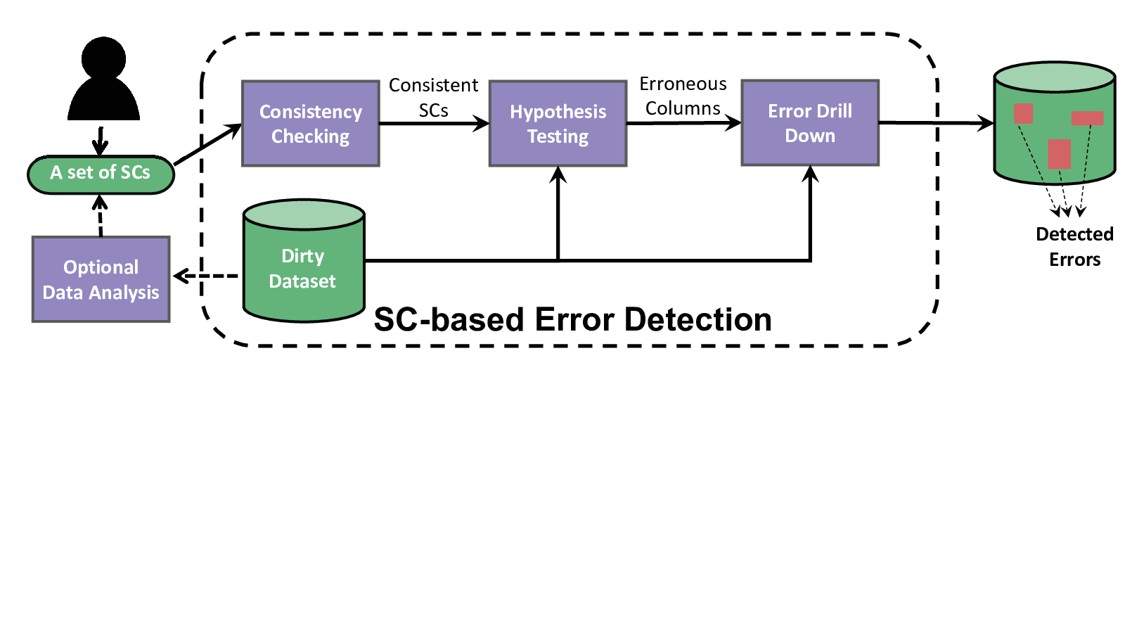
Hypothesis Testing. In the hypothesis testing stage, the system checks for each SC, whether the dataset violates the SC or not. For example, consider and the dataset in Figure 2. The user expects that Model and Color should have an independent relationship. However, a hypothesis test on the data indicates that Model and Color are highly correlated. The user then has a choice to revise the constraint, or to maintain the constraint and have the system mark Model and Color as erroneous columns. Section 5 below discusses hypothesis testing process.
Error Drill Down. If a dataset violates an SC, the user may want to drill down into individual records so that she can understand why an SC is violated and repair the datapoints that caused the violation. Therefore CODED provides an error-drill-down component. The user chooses a violated SC and specifies a threshold . This component returns the top- records that contributes the most to the SC’s violation. Suppose is violated. As will be shown in Section 6, if the user specifies , the system will return , which is a cheap car with high fuel consumption. The user can examine this record and may find out that unlike the other cars, this is a used car. It is worth noting that given the user does not need to write a handcrafted rule like a cheaper car tends to be more fuel-efficient.
5. SC Violation Detection
We study how to detect an SC violation in this section. We first reduce to evaluating marginal SCs in Section 5.1, and then discuss how to apply hypothesis testing to detect the violation of marginal SCs in Section 5.2.
5.1. Reduction to Evaluating Marginal SCs
Evaluating a conditional SC against the data can be reduced to evaluating marginal SCs via the following steps. 1) Reduce testing a complex independence to testing a set of elementary SCs , for each and . 2) If all conditioning variables are categorical, there is a finite set of possible combinations ; conditional independence is equivalent to marginal independence for each (Definition 3.1). If contains continuous variables, we deploy a state-of-the-art data bucketing method in statistics to discretize the data into categorical types with histogram. Discretization groups a number of continuous values into a small number of bins. CODED is open to all the data bucketing methods. Our experiments deployed the methods introduced in (scott2015multivariate). The reported results use the bucketing methods with the best performance (f-score).
Justification. Step 1 can be justified as follows. The decomposition axiom (see Definition 5) shows that in any joint probability distribution, a complex SC entails the corresponding set of pairwise elementary SCs, so this direction entails no loss of generality. The converse is the composition principle, that elementary independencies between single variables can be combined into complex independencies between sets of variables. While this is not true for every probability distribution, Chickering and Meek (Chickering2002) show that the composition property holds for a large class of probability distributions, and provide evidence that real-world datasets satisfy it. Niepert et al. also give formal conditions under which the elementary and general SCs are equivalent (Niepert2013). We can therefore expect that testing complex SCs by decomposing them into elementary SCs will be adequate for error detection in practice.
To evaluate marginal SCs for both and either categorical or numerical, we propose default hypothesis testing methods in the remainder of this section. For the mixed case where is numerical and discrete, we can proceed as follows. For simplicity, assume that is binary 0 or 1. Then we have two continuous conditional distributions and . The independence between and can then be evaluated by testing whether the two conditional distributions are significantly different (uther1998tree).
5.2. Hypothesis Testing
A hypothesis test is a procedure that takes as input a dataset and outputs either 0 (“the hypothesis is rejected") or 1 (“the hypothesis is not rejected"). A statistical hypothesis is rejected when the probability of the data entailed by the hypothesis is below a user-specified threshold. Most hypothesis tests are based on a test statistic , which returns a real number for a dataset. For independence tests, intuitively, the statistic is an aggregate function that summarizes the degree to which the dataset violates the independence hypothesis . The -value specifies the probability of observing a value at least as great as the test statistic for the dataset, assuming the independence constraint:
CODED can deploy any hypothesis tests that specified by users, while including default hypothesis testing methods. To make the paper self-contained, we briefly review the basics of these hypothesis testing methods.
The test measures the (in)dependence among categorical data (pearson1900x). Given an assignment , each datapoint satisfies the assignment or not. The observed count is the number of datapoints that satisfy it. If the sets and were completely independent, the observed counts would equal the product of the marginal counts; these products are called the expected counts: The statistic is calculated as:
The distribution of the chi-square statistic can be approximated by the distribution. That is, we have where and resp. is the number of possible assignments for resp. . We use the statistic for testing independence among discrete (categorical).
Rank Correlations for numeric variables are based on a straightforward intuition: Each variable defines an ordering over data points, and if the variables are associated, the -ordering should carry information about the -ordering. A number of similarity metrics for rankings have been proposed; In this paper, we choose the the most common non-parametric metric Kendall’s as the default method, defined as follows. Consider datapoints with two features . For two datapoints and with , if and , or and , then the two variables agree on the ordering of and and the pair is concordant. The number of concordant pairs is denoted as . Else if and , or and , then the two variables disagree on the ordering of and and the pair is discordant. The number of discordant pairs is denoted as . Pairs neither concordant nor discordant are called tied, and their number is denoted as . The statistic is then computed as
To compute -values, statistical applications use a rescaled denominator, still a function of only , such that the rescaled statistic has an approximately Gaussian distribution.
Comparison. There are many statistics methods (wasserman2013all) that can be applied to verify the independence. We explain why we chose Kendall’s as a default method chosen over other popular options (e.g., Pearson’s coefficient and Spearman’s ). 1) The default method in CODED should be compatible with many data characteristicss, so the fewer underlying data assumptions, the better. In statistical terminology, this means we want to use a non-parametric hypothesis test, which does not that the dependence can be characterized by a fixed set of parameters known a priori before data observation. Pearson’s is a parametric method that measures the degree to which and are linearly related. The disadvantage of the statistic is that it is reliable only under certain assumptions, including that the relationship between and is approximately linear. The computation complexity of Spearman’s is relatively smaller than that of Kendall’s . However, comparison studies (knight1966computer; xu2013comparative; howell2009statistical; croux2010influence; fredricks2007relationship) have found that Kendall’s is generally more robust in avoiding false positives, which makes it preferred for data error detection.
6. Error Drill Down
In this section, we study how to drill down into individual records that contribute the most to the violation of an SC. We first propose a general framework in Section 6.1 and then propose two efficient top-k algorithms for categorical data and numerical data, respectively, in Section 6.2.
6.1. Error-Drill-Down Framework
There are two reasons that motivate the drill-down task. Firstly, an SC violation helps a user to detect which columns have errors, but it does not tell the user which values in the columns may contain the errors. For example, suppose a user specifies an SC: on a car dataset. After a hypothesis test, she finds that Model and Color violate the independent relationship on the dataset. At this point, she knows that there may be some errors in the Model and Color columns. We want to help her to locate the errors in the columns so that she can figure out why the violation happens and then fix the errors.
Secondly, sometimes a dataset has errors, but the errors are not of sufficient magnitude to violate a (in)dependence relationship among columns. We want to leverage SCs to detect the errors even in this situation. For example, consider an SC: . Suppose that after a hypothesis test, the test result indicates that that Fuel and Price are dependent (i.e., no violation) but the dependent relationship is weaker than what she expects. We want to help her investigate why the correlation is weaker than expected.
To this end, we develop an interactive error-drill-down framework. A user specifies an SC and a hypothesis testing method (e.g., test). The framework first applies the hypothesis test to the data, and checks whether SC is violated. If yes, it will return records whose column values are most likely to cause the violation. If no, a user can check whether the returned statistic (e.g., the statistic) is larger or smaller than her expectation. Suppose the statistic is smaller than what she expects. Then, she can use the framework to identify records whose column values are most likely to cause the unexpected result.
Central to this framework is the top-k error detection problem. Let denote a dataset, and denote a hypothesis testing statistic (e.g., the statistic or the statistic). Without loss of generality, we consider only the case where the statistic is larger than a user’s expectation. In this situation, the goal is to find records from such that if they were removed, the test statistic would decrease the most. Definition 2 formally defines the problem.
Definition 2 (Top- Individual Error Detection).
Given a dataset , an SC, a hypothesis testing statistic , and a threshold , we aim to identify a set of records, denoted by , such that is mimized, i.e.,
A naive solution is to enumerate all possibilities, and then return the best result. This is prohibitively expensive. Even with a modest data size of 10,000 records, assuming a reasonable k = 10, this approach would require enumerating possibilities. Therefore, we adopt greedy algorithms to reduce the cost. We propose two greedy algorithms, strategy and strategy. Intuitively, the strategy seeks to directly identify the best records; the strategy seeks to remove the worst records and then return the remaining records as a result.
Strategy. The algorithm first selects the best record from such that if it was removed, the statistic can decrease the most. The algorithm removes from , and then repeats the above process to select the best record from . After iterations, the top- records are identified.
Strategy. The algorithm first selects the worst record from such that if it was removed, the statistic can increase the most. The algorithm removes from , and then repeats the above process to select the worse record from . After iterations, where , the remaining records are returned.
Remark. The strategy is more efficient than the strategy because the former only needs to select records but the latter needs to check records. In terms of effectiveness, the strategy often leads to a better objective value (i.e., smaller because it directly optimizes for that value. The strategy is particularly useful in identifying a set of records that are highly correlated with each other, thus it is more suitable to detect errors for the violation of an independence SC.
6.2. Top-k Error Detection Algorithms
We describe top- error detection methods for the two statistics we examine in this paper, and . We discuss how to implement the strategy for them efficiently. The same implementation can be extended to the strategy trivially.
6.2.1. Categorical Data

We use test as the default method to detect errors for categorical data. We propose an optimization technique to reduce the time of selecting the “best” record at each iteration. The key observation is that if two records have the same values on the tested columns, there is no difference to choose either one of them. Therefore, we can group the records based on the tested columns, and only need to spend time in deciding which group (rather than which record) should be selected at each iteration.
For example, consider an SC: and a dataset similar to Figure 2 but with more records. We first group the records based on the tested columns (i.e., Model and Color). Suppose there are 2 car models and 3 colors. Then, there will be 6 groups in total. Figure 5 illustrates the 6 groups, where the number in each cell represents the total number of the records that belong to that group. Each cell has a value . At each iteration, the strategy only needs to determine which group should be selected and then randomly picks one record from that group based on the statistic . This optimization technique significantly reduces the computational cost since the number of groups could be orders of magnitude smaller than the total number of records.
6.2.2. Numerical Data
We discuss how we employ the framework for numerical data with the test. We formally define the problem as follows.
Definition 3 (-test-based Error Detection).
Given a dataset , an SC, and , the -test-based error detection problem tries to find a subset of records from that contribute the most to the violation of the SC, i.e.,
For simplicity, we denote the count of concordant pairs, discordant pairs, and tied pairs in as , , and , respectively. We omit the denominator of the objective function since it is a constant function of only. The strategy works as follows. At each iteration, it calculates the benefit of each record: Given a record , find all the pairs that contain the record, and then calculate the sum of the weights of these pairs, denoted by . Then, we select the record with the biggest benefit. Once a record is selected, we need to update the benefit of all the remaining records. We use a priority queue to maintain the top- records. Algorithm 1 shows the pseudo-code. Example 6.1 illustrates the algorithm.
; // Returned List
; // A hash table that maps a pair to its weight
for ; 1
for do 3
for to do 10
12
Example 0.
Following the running example in Figure 2, we apply the testing method to detect data errors w.r.t. , and let .
Step 1: Initialization. We calculate the benefit of each record on the entire dataset, and obtain the priority queue . Intuitively, the benefit of a record (e.g., ) means that if was removed, the objective value would be decreased by 9.
Step 2: Removing and Updating. Return the top element of , in this case . Then remove , and update the priority queue. Since shares a zero weight with every other record, the benefit of each record keeps unchanged. The updated queue will be .
Step 3: Repeating Step 2. We repeat Step 2 until records are returned. Here, since , only will be returned.
Efficiency Analysis. The main computational bottleneck of the strategy is the initialization phase. Consider a dataset with two columns: . We need to initialize the benefit of each record. For a single record, this requires comparing with the other records, leading to a time complexity of . Therefore the naive implementation of the initialization phase needs time. This does not scale to large datasets (e.g. 1M records).
The time complexity of the initialization phase can be reduced to with a segment tree. A segment tree is a tree data structure, where each node stores information about a segment. It allows for inserting a segment and querying a segment with both time. To apply this idea, we first sort by column and then scan the records in based on this new order. For each record , we can get the number of concordant pairs of the record by querying the segment of , and the number of discordant pairs by querying the segment of . Once the two numbers are obtained, we insert a segment (representing a single point) to the tree. We need time to process each record, thus the total time complexity is . With this optimization, error drill-down can handle a dataset with millions of records. Further details are in Appendix A.
7. Consistency Checking
In this section, we first define the consistency checking problem, then discuss different approaches for different types of constraints. Intuitively, if a set of SCs is consistent, it means that has no conflict. That is, there exists a joint distribution that satisfies .
Definition 4 (Consistency).
Given a set of SCs, let denote the set of random variables that appear in . The consistency problem is to determine whether there exists a joint distribution that satisfies every SC in .

For example, consider . Since there are three random variables in , we have . As shown in Figure 6, we can construct a joint distribution that satisfies , thus is consistent. If we are given , it is impossible to construct a joint distribution that satisfies , thus is inconsistent.
For complete models and elementary saturated constraints (Section 3.3), consistency checking is easy. (1) SCs represented in a complete model structure is guaranteed to be consistent because parametrizing the elicited model defines a probability distribution that satisfies the constraints. (2) For SCs statements that are saturated and elementary, Heckerman et al. show that a set of SCs is consistent if and only if it satisfies the symmetry axiom described in Section 5 (Heckerman2000), which is easy to check. We therefore focus our discussion on general SCs.
7.1. Consistency Checking By Inference
Determining the consistency of general SC statements is a very difficult problem; it is not even known whether it is decidable (Niepert2013). Nonetheless, AI researchers have developed a number of heuristic approaches (Niepert2013; pearl2; studeny1990conditional). A principled approach is to use an inference framework for deriving a contradiction (pearl2), as illustrated in Algorithm 2. A similar inference framework is used to check the consistency of a set of functional dependencies (bohannon2007conditional). For example, consider . We have and . We can see that does not imply , thus is consistent.
Once an inconsistency is derived by implication, the derivation can help the user to resolve the inconsistency. Specifically, suppose that the consistency-checking algorithm finds a conflict: implies but is in . We ask the user to check which one is correct. If the former is correct, we remove from . Otherwise, we show the derivation of from and then ask the user to remove the incorrect SCs involved in the derivation. The implication approach requires an inference system for Independence SCs, which we describe next.
The Graphoid Axioms for Independence SCs. A commonly used set of axioms is Geiger and Pearl’s system (pearl2).
Definition 5.
Let , , , and denote four disjoint sets of random variables. The graphoid axioms are the following:
Symmetry:
Decomposition:
Weak Union:
Contraction:
Note that can be the empty set. For example, for the symmetry axiom, we have
Example. Suppose we are given three constraints:
Applying the Contraction rule to and :
Applying the Decomposition rule to :
Then, we can see that is inconsistent with the given . Therefore, is inconsistent.
Soundness and Completeness. Traditional functional dependencies (FDs) have a sound and complete inference system that is known as Armstrong’s Axioms (abiteboul1995foundations). Wenfei et al. extend Armstrong’s Axioms to CFDs and prove that the new inference system is also sound and complete (bohannon2007conditional), but deciding the consistency of a set of CFDs is NP-hard. Unfortunately, inference for SCs is a hard problem: a major negative result due to Studeny says that no finite set of axioms is both sound and complete for general SCs (studeny1990conditional). The system is sound (pearl2) (for strictly positive joint probability distributions), but by Studeny’s result, not complete. The situation for general SCs is thus comparable to that for DCs, where we currently have a set of sound (but not complete) inference rules (chu2013holistic). Niepert et al. introduce another set of axioms for SCs, which is complete but not sound (Niepert2013). They suggest applying both and to a given set of constraints, which allows the implication algorithm to both falsify some cases of inconsistent SCs (via ) and validate some cases of consistent SCs (via ). We leave evaluating system for future work.
Time Complexity.
We next show that the inference method based on system is efficient if the number of variables that appear in any of the input SCs is relatively small.
To analyze the time complexity of the implication algorithm, we answer two questions:
Q1. What is the time complexity of generating a new SC?
Q2. How many new SCs can be generated in total?
For , consider the two inference rules in Definition 5. For the rules with a single left-hand SC, the algorithm can check each derived SC for whether it can be used to generate a new SC. The time complexity of this process is . For the rules with two left-hand SCs, a simple approach is to enumerate every pair of SCs in and then check whether the rule can be used or not, requiring time. In total, our algorithm needs time to generate a new SC at each iteration.
For , we seek to compute an upper bound for the number of newly generated SCs. The key observation is that for any inference rule in , every variable that occurs on the right-hand SC also occurs on the left-hand side. For example, in the contraction rule, four sets of variables occur on the left-hand side, and the same four sets on the right-hand side. We say covers if the variable set of is a superset of the variable set of . For a fixed set of variables, there are possible SCs with these variable (depending on whether each variable is assigned to the first set, the second set, or the conditioning set). Given the key observation, we can therefore bound the number of generated by a single SC as (Each SC must involve at least two variables.) Overall the number of number of generated can therefore be bounded by , where is the largest number of variables that occurs in any of the input . This shows that the computational cost of the implication algorithm is pseudo-polynomial in the number of input and the parameter , meaning polynomial if is small enough to be treated as a constant (Garey1979).
8. Experiments
| Attributes | CODED | Denial Constraints |
|---|---|---|
| N_oxide(N), Distance(D) | For any two records and , if , then | |
| Rooms(R), Black Index(B) | ||
| Tax rate, Black Index, Crime(C) | For any and with , if , then | |
| N_oxide, Black Index, Tax rate (T) | ||
| Buying Price(BP), Class(Cl) | For any two records and , if , then | |
| Safety(SA), Doors(DR) | ||
| Temperatures (T) of Sensor 8 and Sensor 9 | For any two and , if , then | |
| Games(G), Goal Plus-Minus(GPM), Year(Y) |
We evaluate the effectiveness and efficiency of our methods on real-life datasets with both synthetic errors and real errors. Specifically, we examine (1) the computational efficiency of the consistency-checking methods, (2) the effectiveness of our method compared to the state-of-the-art approaches on detecting synthetic and real-life errors, and (3) the scalability of our error-detection method.
8.1. Experiment Setup
Datasets. We evaluated our approaches on five real datasets.
(1) BOSTON11 1 https://www.cs.toronto.edu/ delve/data/boston/bostonDetail.html. The Boston dataset was taken from the Boston Standard Metropolitan Statistical Area (SMSA) in 1970. This dataset was first used in (Harvard) to study the relationship between clean air quality and household’s willing to pay. There are 506 instances, and each instance has 14 attributes. We used attributes: Distance to CBD area-Distance (D), Nitric Oxides Concentration-N_oxide (N), Crime Rate-Crime (C), Black index of population(B), Rooms(R) and Tax Rate(T).
(2) CAR22 2 https://archive.ics.uci.edu/ml/datasets/Car+Evaluation.. The Car Evaluation dataset is from UCI Machine Learning repository. This dataset contains seven attributes. We used 4 attributes: Buying price(BP), Car Class (CL), Doors(DR), and Safety level(SA).
(3) HOSP33 3 http://www.hospitalcompare.hhs.gov. The HOSP dataset contains 100K records with 19 attributes. It was used in previous data-cleaning studies(chu2013holistic; DBLP:journals/pvldb/RekatsinasCIR17). We got the clean and dirty versions of the dataset from (chu2013holistic).
(4) SENSOR44 4 http://db.csail.mit.edu/labdata/labdata.html. The Sensor dataset collected the sensor reports from the Berkeley/Intel Lab. The dataset has more than 2 million records, containing the humidity and temperature reports from 54 different sensors.
(5) HOCKEY55 5 https://github.com/liuyejia/Model_Trees_Full_Dataset documents clean and dirty versions.. The Hockey dataset collected the records of each NHL game from 1998-2010. It has more than ten attributes which variously describe player attributes and player performance statistics for a season.
Simulated Errors. The purpose of the use of simulated errors is to help us gain a deep understanding of the effectiveness of our approach in various situations. We simulated two types of errors: sorting error and imputation error. As shown in Section 1, both types of errors have appeared in reality.
For the sorting error, we selected of column (randomly or based on column ) and sort its values in an ascending order; for the imputation error, we selected of column (randomly or based on column ) and replaced them with the mean value of column A. is called error rate. Note that the sorting error (the imputation error) may either make two columns and more independent or less independent based on whether the values are selected randomly or based on column . We used random selection for dependence SCs, column for independence SCs. We also explored the combined impact of the two error types. Our combination error consists of 80% sorting error and 20% imputation error.
Real-life Errors. The Sensor and Hockey datasets contain real-life errors. To compress the Sensor dataset, we replaced sensor readings by their hourly average. The aggregated dataset has many outliers. Since some outliers are very easy to detect, we considered the following scenario to make the experiment more challenging. Consider two data scientists: Alice and Bob. Alice first removed easy-to-detect outliers (e.g., temperature > 100 °C) and replaced them with the mean temperature. When Bob got the dataset from Alice, he did not know that the raw dataset was changed by Alice. Imagine Bob wanted to use the dataset differently (e.g., count the outliers in the raw dataset). In this situation, Bob wanted to detect not only the remaining outliers but also the outliers removed by Alice. The ground-truth of the dataset was obtained using the method in (jeffery2006declarative).
Hockey is a public dataset used for hockey data analytics. We originally thought that the dataset had no error. However, our hockey knowledge specified an SC, (last row in Table 4), which we noted was violated in the table. It turned out that the dataset provider filled all the missing values with 0 or mean values. The correct ground-truth of the dataset was obtained from other reliable hockey websites.
Error-Detection Approaches. We compared CODED with three state-of-the-art error detection approaches.
Denial Constraints (DC) (chu2013discovering) is an integrity constraint based error detection approach. The original DC approach does not support top- error detection. We extended it as follows: for each record , count the number of other records that are inconsistent with given the DC. Then return the top- records that involve the most number of violations. Table 4 summarizes the constraints used by DC. ‘‘ means that we cannot find a DC to represent the same independence relationship as CODED (cf. Section 3.2).
DBoost (mariet2016outlier) is the state-of-the-art outlier detection approach. This is also used by (abedjan2016detecting) to compare different types of error-detection approaches. We used an implementation available online66 6 https://github.com/cpitclaudel/dBoost. We applied DBoost with three models: GMM, Gaussian and Histogram. For categorical data, we employed the bin width that achieves the best f-score results. For numeric data, we employed Gaussian and GMM with the mixture parameter nsubpops threshold set at , and the statistical epsilon to be .
Approximate Functional Dependency(AFD) (mandros2017discovering) is an error detection approach based on approximate constraints. To make AFD support top- error detection, we extended it by returning the top- records that lead to the most number of violations. We considered two AFDs on the HOSP dataset Zipcode -> City and Zipcode -> State, and compared with CODED w.r.t. Zipcode City and Zipcode State.
CODED is our SC-based error detection approach. Table 4 summarized the constraints used by CODED. For the CODED hypothesis testing, we used the test for categorical data, and the test for numerical data. We implemented the error-drill-down framework, and adopted the strategy for dependence SCs and the strategy for independence SCs.
Quality Measurement. We considered two user scenarios. (i) The user wants to manually examine a small number of records (e.g., ) in order to reason about data errors. For this scenario, since is fixed, we need to maximize Precision@K, which is defined as the ratio of the number of correctly detected records to the number k. (ii) The user wants to detect all errors in order to repair them. For this scenario, as increases, recall increases while precision potentially decreases. We report Precision@K, Recall@K, and F-score@K by varying. Precision@K is the same as above. Recall@K is the ratio of the number of correctly detected records among the returned records to the number of total erroneous records, and F-score@K is their harmonic mean.
8.2. Experimental Results
Exp-1: Efficiency of Consistency Checking. We examined the efficiency of the consistency-checking algorithm. Note that consistency checking is not related to data. Therefore, randomly generating SCs is appropriate to test the scalability of our consistency-checking algorithm. We randomly generated independence SCs and dependence SCs containing up to 3 out of variables, where SCs are elementary CIs (See Table 2). We measured the runtime of consistency checking by varying and , respectively. The results are shown in Figure 7. Each figure has three lines, which represent different ratios of to .
We make two interesting observations. First, our consistency-checking algorithm scales well by varying either or . Even with 500 independence (dependence) SCs, the algorithm can terminate within 0.5 ms. Second, the computation time is more related to than . This is because the consistency-checking algorithm proposed comprises two parts: implication and checking, where the implication algorithm needs time, which typically dominates the whole process.


Exp-2: Impact of Errors. To illustrate the impact of data errors, we varied the error rates of sorting error, imputation error, and combination error, and tested how the absolute tau value (i.e., ) changed accordingly. Recall that a larger implies a more dependent relationship. We selected two SCs, (R/B in Figure 9 ) and (N/D in Figure 9).
Figure 9 shows the results w.r.t. an independence SC. All errors tend to raise , indicating a violation of the independence SC. The sorting error has a consistent effect on the tau value (Figure(a)). Imputation error has a strong negative impact at lower error rates, then the tau value reverses (Figure(b)). This can be explained as follows. Starting with two independent columns (i.e., a very small ), imputing a constant value induces more correlation between the two columns (i.e., a larger ). Once many records have been imputed with a constant value, the correlation decreases until one column contains the same constant everywhere, implying zero correlation between them (i.e., ).
Figure 9 shows the results w.r.t. a dependence SC. As more errors were generated, decreased, so the columns were evaluated as more independent. With the error rate at 0.8, approached zero, indicating an independence relationship.
Exp-3: Evaluation of Error-Detection Approaches. We compared CODED with existing error-detection methods on the Boston dataset. For dependence SCs, we compared with DC and DBoost; for independence SCs, since DC cannot express independence relationships (cf. Section 3.2), we compared only with DBoost. We considered both marginal and conditional SCs, as summarized in Table 4.
Marginal SCs: and . Figure 11 and Figure 11 show the results for and , respectively. We consider three error levels, depending on the average error rate for the column: minor error = , moderate error = , and major error = . We reported precision@50.
We first examine CODED’s performance. CODED’s precision increases with the error level. The reason is that when there is a larger portion of errors, the degree of dependence/independence changes more, thus it is easier for CODED to detect violations.
We next compared the performance of CODED, DC and DBoost. As shown in Figure 11 and Figure 11, CODED outperformed the other two approaches. DC did not perform well because the specified denial constraint (i.e., if , then ) did not always hold, which led to many false positives. CODED outperformed DBoost due to two reasons. First, DBoost derived correlations from dirty data, and then leveraged the derived correlations to detect errors. However, since data is dirty, the derived correlations might be wrong. Second, DBoost is designed to detect outliers but the dataset has erroneous values (e.g., imputed mean values) that look like a normal value. Thus, DBoost failed to detect these errors.
We compared the F-score of CODED, DC and DBoost using different values (moderate error level). Results are shown in Figure 14 and Figure 14 for and , respectively. We can see that CODED achieved significant higher F-score than DC and DBoost for all settings. CODED’s performance depends on the error type: It performed better for sorting error and combination error, where the average F-score is and the max F-score is around . But for imputation error, the average F-score and the max F-score decrease to and , respectively. As we explained above, if errors have a small impact on SCs, the power of using SCs to detect the errors decreases.
Conditional SCs: and . We also examined the effectiveness of CODED for conditional dependence and independence SCs, with moderate error level. The results are very similar to non-conditional cases (see Appendix C for more detail).
Exp-4: Effectiveness on Categorical Data. So far, we have only focused on numerical data using the test. Next, we use the test and evaluate the effectiveness of CODED on categorical data. The conclusion is that CODED outperformed DBoost in terms of F-score for both independence and dependence SCs. Due to the space limit, please refer to the Appendix D for more details.
Exp-5: Effectiveness compared with AFD. We compared the effectiveness of CODED and AFD on the HOSP dataset. Figure 12(a) shows the result for Zipcode -> City vs. Zipcode City; Figure 12(b) shows the result for Zipcode -> State vs. Zipcode State.
We have a number of interesting observations. First, CODED and AFD got the same F-score for . This is because both of them achieved 100% precision and the same recall when . Second, CODED’s F-score continued to grow when but AFD’s F-score started to decrease. This is because that AFD can only detect the errors on the right-hand side (i.e., City or State) of an AFD. If an error occurs on the left-hand side (i.e., Zipcode), AFD cannot detect the errors. In contrast, CODED considers the statistical relationship between two columns, therefore it can detect the errors in both columns.


Exp-6: Effectiveness with Real-life Errors. We evaluated CODED on the datasets with real-life errors.
Sensor Dataset (). Neighboring sensors tend to report similar temperatures, which means that their readings of the temperature should be dependent. We specified a dependence SC between the readings of Sensor 8 and Sensor 9. Figure 16 shows the experimental result. The average Precision of CODED, DC, and DBoost was , and , respectively. Unlike the other two methods, the precision of CODED never decreased. and maintained a high precision around . For Recall and F-score, all three approaches increased continuously. CODED outperformed the other two methods with a higher increasing speed. This experiment validated the effectiveness of CODED when using it to detect real-world errors w.r.t. dependence SCs.
Hockey Dataset (). For the Hockey dataset, the columns Games(G) and Goal Plus-Minus(GPM) should be independent given Draft Year(Y), because hockey draft studies have shown that the total number of professional games played by a player is independent of their Plus-Minus before they joined the professional league. We specified an independence SC: . Figure 16 shows the experimental result. We only compared CODED with DBoost since DC cannot express independencies. We can see that CODED outperformed DBoost in terms of Precision, Recall, and F-score. In particular, when k = 50, DBoost only got a precision of 0.28, but the precision of CODED was 0.68 (around 2.5 ) higher. This experiment validated the effectiveness of CODED when using it to detect real-world errors w.r.t. independence SCs.
Exp-7: Scalability. Our evaluation provided evidence that error drill down scales well in terms of both and . Please refer to Appendix B for more details.
9. Conclusion and Future Work
A statistical constraint (SC) represents a probabilistic association, or its absence, among columns in a data table. SCs provide a powerful expressive formalism for capturing a user’s domain knowledge. This paper explored how to exploit SCs in data cleaning, by identifying the data errors that lead to their violation. We compared SCs and traditional integrity constraints, and identified types of situations where SCs add expressive power: when the user wishes to assert the irrelevance of one set of columns to another, and when the user expects an inferential relationship between columns to hold not precisely, but only approximately to a certain degree, with exceptions. Our CODED system leverages SCs for error detection by addressing three challenges: For SC violation detection, we showed how well-established statistical metrics ( and Kental’s ) can be used to quantify the degree to which an SC is violated. To explain violations, we proposed an error-drill-down framework, and devised efficient algorithms to identify the top- records that contribute the most to the violation of an SC. For checking the consistency of a set of input SCs, we described an inference-based consistency-checking algorithm, which is pseudo-polynomial in terms of the number of input SCs and the largest number of variables that occurs in any of the input SCs. We conducted extensive experiments on real-world datasets with both synthetic and real-life errors, as well as a range of constraint types. The results showed that SCs were effective in detecting data errors that violate them, compared to state-of-the-art approaches.
CODED represents a novel approach to leverage powerful statistical methods for error detection. It has great potential to be useful in practice, and opens a new set of research directions in the intersection of statistics and data management. In the future, we plan to extend CODED from two aspects. (1) Human-in-the-Loop. Integrate the discovery and validation of SCs to help the user to discover and validate them efficiently. (2) Data Repairing. Extend CODED to the error-repairing stage, to automatically repair errors so that the cleaned data satisfies a set of given SCs.
Appendix A Efficient Implementation for Strategy
We discuss the efficient Implementation of the strategy detailed here. As illustrated in Section 6.2, we choose another data structure segment tree in the initialization phase so as to greatly reduce the time complexity. Before applying this idea, some pre-processing is needed. We first sort dataset by column. Then we scan the new data set to obtain the concordant pairs, and non-concordant pairs. Later, we insert a segement tree to the segment tree. After the initialization phase, we continue do the iterations as shown in the Algorithm 3. Algorithm 3 illustrates the pseudo-code. This efficient implementation is also applicable to strategy.
Appendix B Scalability.
We replicated the Boston dataset to enlarge its data size, and chose a dependence: SC . We examined the execution time of CODED by varying and (# Records), respectively. The results are shown in Figure 17.
Recall that the time complexity of CODED (the strategy) is for initialization, and is for selecting records. The results are consistent with the complexity analysis, and demonstrate the good scalability of CODED w.r.t. and .

; // Priority Queue
; // Returned List
for ; 1
for do 3
for to do 10
12


Appendix C Effectiveness on Conditional Independence SCs
and . We also examined the effectiveness of CODED for conditional dependence and independence SCs, with moderate error level. Constraints used for CODED, DC and DBoost are summarized in Table 4. To accommodate the variables of constraints to CODED framework, we further bucket the value of Tax Rate into categorical values. We categorize the numerical value into buckets following its distribution. We reported their F-score under different values at moderate error level, which is similar to Exp-3. Results are shown in Figure 19 and Figure 19 respectively. CODED obtained a higher F-score than another two state-of-art methods, which is even more significant under independence SCs. Also, similar to Exp-3 and Exp-4, the detection effectiveness of imputation error is not as stable as that of another two types errors. The average F-score of CODED under independence SCs is and with max F-score , however the two results will decrease to and with imputation error inserted. This again demonstrates that the CODED can detect the power of errors as if the power is not as significant, CODED is not that powerful.

Appendix D Effectiveness on Categorical Data.
We use the test and evaluate the effectiveness of CODED on categorical data. We selected two SCs ( and ) on the Car dataset. DC is not applicable here because there are too many violations for the feasible DCs that we constructed. We compared the performance of CODED and DBoost at the moderate error level. Figure 20 shows the results. Due to the space limit, we just focus on the imputation errors in this experiment. The average F-score of CODED and DBoost are and , respectively. Similar to Exp-3, CODED outperformed DBoost in terms of F-score for both independence and dependence SCs.
References
- [1] The Four V’s of Big Data. Accessed: 2018-02-28.
- [2] Z. Abedjan, X. Chu, D. Deng, R. C. Fernandez, I. F. Ilyas, M. Ouzzani, P. Papotti, M. Stonebraker, and N. Tang. Detecting data errors: Where are we and what needs to be done? Proceedings of the VLDB Endowment, 9(12):993–1004, 2016.
- [3] S. Abiteboul, R. Hull, and V. Vianu. Foundations of databases: the logical level. Addison-Wesley Longman Publishing Co., Inc., 1995.
- [4] M. Bergman, T. Milo, S. Novgorodov, and W. C. Tan. Query-oriented data cleaning with oracles. In ACM SIGMOD, pages 1199–1214, 2015.
- [5] P. Bohannon, W. Fan, M. Flaster, and R. Rastogi. A cost-based model and effective heuristic for repairing constraints by value modification. In Proceedings of the 2005 ACM SIGMOD international conference on Management of data, pages 143–154, 2005.
- [6] P. Bohannon, W. Fan, F. Geerts, X. Jia, and A. Kementsietsidis. Conditional functional dependencies for data cleaning. In Data Engineering, 2007. ICDE 2007. IEEE 23rd International Conference on, pages 746–755. IEEE, 2007.
- [7] P. Bohannon, M. Flaster, W. Fan, and R. Rastogi. A cost-based model and effective heuristic for repairing constraints by value modification. In SIGMOD, pages 143–154, 2005.
- [8] F. Chiang and R. J. Miller. Discovering data quality rules. Proceedings of the VLDB Endowment, 1(1):1166–1177, 2008.
- [9] F. Chiang and R. J. Miller. A unified model for data and constraint repair. In Data Engineering (ICDE), 2011 IEEE 27th International Conference on, pages 446–457. IEEE, 2011.
- [10] D. M. Chickering and C. Meek. Finding optimal Bayesian networks. In UAI, pages 94–102, 2002.
- [11] X. Chu, I. F. Ilyas, S. Krishnan, and J. Wang. Data cleaning: Overview and emerging challenges. In Proceedings of the 2016 International Conference on Management of Data, pages 2201–2206. ACM, 2016.
- [12] X. Chu, I. F. Ilyas, and P. Papotti. Discovering denial constraints. Proceedings of the VLDB Endowment, 6(13):1498–1509, 2013.
- [13] X. Chu, I. F. Ilyas, and P. Papotti. Holistic data cleaning: Putting violations into context. In Data Engineering (ICDE), 2013 IEEE 29th International Conference on, pages 458–469. IEEE, 2013.
- [14] X. Chu, J. Morcos, I. F. Ilyas, M. Ouzzani, P. Papotti, N. Tang, and Y. Ye. Katara: A data cleaning system powered by knowledge bases and crowdsourcing. In Proceedings of the 2015 ACM SIGMOD International Conference on Management of Data, pages 1247–1261. ACM, 2015.
- [15] R. G. Cowell, P. Dawid, S. L. Lauritzen, and D. J. Spiegelhalter. Probabilistic networks and expert systems: Exact computational methods for Bayesian networks. Springer Science & Business Media, 2006.
- [16] C. Croux and C. Dehon. Influence functions of the spearman and kendall correlation measures. Statistical methods & applications, 19(4):497–515, 2010.
- [17] K. Das, J. Schneider, and D. B. Neill. Anomaly pattern detection in categorical datasets. In Proceedings of the 14th ACM SIGKDD international conference on Knowledge discovery and data mining, pages 169–176. ACM, 2008.
- [18] K. Das and J. G. Schneider. Detecting anomalous records in categorical datasets. In Proceedings of the 13th ACM SIGKDD International Conference on Knowledge Discovery and Data Mining, San Jose, California, USA, August 12-15, 2007, pages 220–229, 2007.
- [19] T. Dasu and J. M. Loh. Statistical distortion: Consequences of data cleaning. Proceedings of the VLDB Endowment, 5(11):1674–1683, 2012.
- [20] A. P. Dawid. Conditional independence in statistical theory. Journal of the Royal Statistical Society. Series B (Methodological), pages 1–31, 1979.
- [21] R. Fagin. Multivalued dependencies and a new normal form for relational databases. ACM Transactions on Database Systems (TODS), 2(3):262–278, 1977.
- [22] G. A. Fredricks and R. B. Nelsen. On the relationship between spearman’s rho and kendall’s tau for pairs of continuous random variables. Journal of statistical planning and inference, 137(7):2143–2150, 2007.
- [23] M. R. Garey and D. S. Johnson. Computers and Intractability: A Guide to the Theory of NP-Completeness. W. H. Freeman Co., 1979.
- [24] D. Geiger and J. Pearl. Logical and algorithmic properties of conditional independence and graphical models. The Annals of Statistics, pages 2001–2021, 1993.
- [25] M. Hall, E. Frank, G. Holmes, B. Pfahringer, P. Reutemann, and I. H. Witten. The weka data mining software: an update. SIGKDD Explorations, 11(1):10–18, 2009.
- [26] D. Harrison and D. L. Rubinfeld. Hedonic housing prices and the demand for clean air. Journal of environmental economics and management, 5(1):81–102, 1978.
- [27] D. Heckerman, D. M. Chickering, C. Meek, R. Rounthwaite, C. Kadie, and P. Kaelbling. Dependency networks for inference, collaborative filtering, and data visualization. Journal of Machine Learning Research, 1:49–75, 2000.
- [28] J. M. Hellerstein. Quantitative data cleaning for large databases. United Nations Economic Commission for Europe (UNECE), 2008.
- [29] D. C. Howell. Statistical methods for psychology. Cengage Learning, 2009.
- [30] Z. Huang and Y. He. Auto-detect: Data-driven error detection in tables. In Proceedings of the 2018 ACM SIGMOD International Conference on Management of data. ACM, 2018.
- [31] I. F. Ilyas and X. Chu. Trends in cleaning relational data: Consistency and deduplication. Foundations and Trends in Databases, 5(4):281–393, 2015.
- [32] I. F. Ilyas, V. Markl, P. Haas, P. Brown, and A. Aboulnaga. Cords: automatic discovery of correlations and soft functional dependencies. In Proceedings of the 2004 ACM SIGMOD international conference on Management of data, pages 647–658. ACM, 2004.
- [33] S. R. Jeffery, G. Alonso, M. J. Franklin, W. Hong, and J. Widom. Declarative support for sensor data cleaning. In International Conference on Pervasive Computing, pages 83–100. Springer, 2006.
- [34] W. R. Knight. A computer method for calculating kendall’s tau with ungrouped data. Journal of the American Statistical Association, 61(314):436–439, 1966.
- [35] S. Kolahi and L. V. S. Lakshmanan. On approximating optimum repairs for functional dependency violations. In Database Theory - ICDT 2009, 12th International Conference, St. Petersburg, Russia, March 23-25, 2009, Proceedings, pages 53–62, 2009.
- [36] S. Krishnan, M. J. Franklin, K. Goldberg, J. Wang, and E. Wu. Activeclean: An interactive data cleaning framework for modern machine learning. In Proceedings of the 2016 International Conference on Management of Data, pages 2117–2120. ACM, 2016.
- [37] S. Krishnan, J. Wang, M. J. Franklin, K. Goldberg, T. Kraska, T. Milo, and E. Wu. Sampleclean: Fast and reliable analytics on dirty data. IEEE Data Eng. Bull., 38(3):59–75, 2015.
- [38] S. Lopes, J.-M. Petit, and L. Lakhal. Efficient discovery of functional dependencies and armstrong relations. In International Conference on Extending Database Technology, pages 350–364. Springer, 2000.
- [39] P. Mandros, M. Boley, and J. Vreeken. Discovering reliable approximate functional dependencies. In Proceedings of the 23rd ACM SIGKDD International Conference on Knowledge Discovery and Data Mining, pages 355–363. ACM, 2017.
- [40] Z. Mariet, R. Harding, S. Madden, et al. Outlier detection in heterogeneous datasets using automatic tuple expansion. 2016.
- [41] C. Mayfield, J. Neville, and S. Prabhakar. Eracer: a database approach for statistical inference and data cleaning. In Proceedings of the 2010 ACM SIGMOD International Conference on Management of data, pages 75–86. ACM, 2010.
- [42] M. Niepert, M. Gyssens, B. Sayrafi, and D. Van Gucht. On the conditional independence implication problem: A lattice-theoretic approach. Artificial Intelligence, 202:29–51, 2013.
- [43] J. Pearl. Causality: Models, Reasoning, and Inference. Cambridge university press, 2000.
- [44] K. Pearson. X. on the criterion that a given system of deviations from the probable in the case of a correlated system of variables is such that it can be reasonably supposed to have arisen from random sampling. The London, Edinburgh, and Dublin Philosophical Magazine and Journal of Science, 50(302):157–175, 1900.
- [45] N. Prokoshyna, J. Szlichta, F. Chiang, R. J. Miller, and D. Srivastava. Combining quantitative and logical data cleaning. PVLDB, 9(4):300–311, 2015.
- [46] V. Raman and J. M. Hellerstein. Potter’s wheel: An interactive data cleaning system. In VLDB, pages 381–390, 2001.
- [47] T. Rekatsinas, X. Chu, I. F. Ilyas, and C. Ré. Holoclean: Holistic data repairs with probabilistic inference. PVLDB, 10(11):1190–1201, 2017.
- [48] F. Riahi and O. Schulte. Model-based outlier detection for object-relational data. In Computational Intelligence, 2015 IEEE Symposium Series on, pages 1590–1598. IEEE, 2015.
- [49] S. Rosset, C. Perlich, G. Świrszcz, P. Melville, and Y. Liu. Medical data mining: insights from winning two competitions. Data Mining and Knowledge Discovery, 20(3):439–468, 2010.
- [50] S. Roy and D. Suciu. A formal approach to finding explanations for database queries. In SIGMOD, pages 1579–1590, 2014.
- [51] B. Salimi, C. Cole, P. Li, J. Gehrke, and D. Suciu. Hypdb: a demonstration of detecting, explaining and resolving bias in olap queries. Proceedings of the VLDB Endowment, 11(12):2062–2065, 2018.
- [52] B. Salimi, J. Gehrke, and D. Suciu. Bias in OLAP queries: Detection, explanation, and removal. In ACM SIGMOD, pages 1021–1035, 2018.
- [53] D. W. Scott. Multivariate density estimation: theory, practice, and visualization. John Wiley & Sons, 2015.
- [54] P. Spirtes, C. Glymour, and R. Scheines. Causation, Prediction, and Search. MIT Press, 2000.
- [55] M. Studeny. Conditional independence relations have no finite complete characterization. 1990.
- [56] W. T. Uther and M. M. Veloso. Tree based discretization for continuous state space reinforcement learning. In Aaai/iaai, pages 769–774, 1998.
- [57] X. Wang, X. L. Dong, and A. Meliou. Data x-ray: A diagnostic tool for data errors. In Proceedings of the 2015 ACM SIGMOD International Conference on Management of Data, Melbourne, Victoria, Australia, May 31 - June 4, 2015, pages 1231–1245, 2015.
- [58] X. Wang, A. Meliou, and E. Wu. Qfix: Diagnosing errors through query histories. In Proceedings of the 2017 ACM International Conference on Management of Data, pages 1369–1384. ACM, 2017.
- [59] L. Wasserman. All of statistics: a concise course in statistical inference. Springer Science & Business Media, 2013.
- [60] E. Wu and S. Madden. Scorpion: Explaining away outliers in aggregate queries. Proceedings of the VLDB Endowment, 6(8):553–564, 2013.
- [61] C. Wyss, C. Giannella, and E. Robertson. Fastfds: A heuristic-driven, depth-first algorithm for mining functional dependencies from relation instances extended abstract. In International Conference on Data Warehousing and Knowledge Discovery, pages 101–110. Springer, 2001.
- [62] W. Xu, Y. Hou, Y. Hung, and Y. Zou. A comparative analysis of spearman’s rho and kendall’s tau in normal and contaminated normal models. Signal Processing, 93(1):261–276, 2013.
- [63] M. Yakout, L. Berti-Équille, and A. K. Elmagarmid. Don’t be scared: use scalable automatic repairing with maximal likelihood and bounded changes. In Proceedings of the 2013 ACM SIGMOD International Conference on Management of Data, pages 553–564. ACM, 2013.
- [64] C. Yan and Y. He. Synthesizing type-detection logic for rich semantic data types using open-source code. In Proceedings of the 2018 ACM SIGMOD International Conference on Management of data. ACM, 2018.