Towards Higher Spectral Efficiency: Spatial Path Index Modulation Improves Millimeter-Wave Hybrid Beamforming

In this paper we consider a point-to-point communication system via mmWave with $N_{\text{t}}$ transmit antennas (TAs) and $N_{\text{r}}$ receive antennas (RAs). To better illustrate the proposed system structure, we depict the corresponding system model in Fig. 1. As can be seen from the figure, the major difference between SPIM-mmWave system and the conventional system is that a set of RF switches are imposed between the outputs of RF chains and the inputs of ABF. For a transmitter with $N_{\text{s}}\geq 1$ RF chains, we assume that the ABF can maximally process $M\geq N_{\text{s}}$ inputs, while each of the $M$ inputs is connected to the $N_{\text{t}}$ TAs via a complete independent set of phase shifters. In this paper, we consider a massive-MIMO scenario, thus implying that $N_{\text{t}}\gg 1$ as well as $N_{\text{t}}>M$. For the purpose of convenience, in the remainder of this paper we refer $M$ as the number of spatial paths, which represents the maximum number of available spatial transmission channels (but cannot be all simultaneously exploited due to the limitation of RF-chain number). We assume that $M\geq N_{\text{s}}$ throughput this paper. More importantly, in the case of $M>N_{\text{s}}$, there exists $\binom{M}{N_{\text{s}}}$ choices of connections between the RF chains and ABF. Therefore we incorporate an extra stream of information, i.e. the spatial-domain information (represented by $x_{0}$, as depicted in Fig. 1) to randomly assign the outputs of RF chains to the $M$ taps, which is in accordance to the principle of IM, i.e. an information-driven random switching regime. Lastly, we assume that the user takes in $S\geq 1$ independent symbol streams, which are linked to the $N_{\text{s}}$ RF chain outputs using a $N_{\text{s}}\times S$ DBF matrix. To fully exploit spatial multiplexing gain, we require that $S=N_{\text{s}}$ in this paper.

It can thus be seen that, when $M=N_{\text{s}}$, the proposed SPIM-mmWave MIMO system reduces to a conventional mmWave-MIMO system with HBF as in [22] (in this case the spatial-domain information is also absent since there is only one choice of connection). When $M>N_{\text{s}}$, the proposed system becomes an IM-assisted mmWave-MIMO system as in [18], which literally performs IM with respect to the $M$ spatial paths, in which a part of information is encoded onto the specific indices of spatial paths that are utilized for information transmission. Therefore the proposed system incorporates both conventional and IM-assisted mmWave MIMOs as its special cases.

To facilitate our theoretic analysis, we let $\mathbf{x}\in\mathbb{C}_{N_{\text{s}}\times 1}$ represent the transmitted symbol vector that is fed to DBF. Similar to many of the current research, it is assumed that $\mathbf{x}$ is subject to a multi-variate complex-valued Gaussian distribution, i.e. $\mathbf{x}\sim\mathcal{CN}(\mathbf{0},\mathbf{I}_{N_{\text{s}}})$. Furthermore, we use $\mathbf{D}\in\mathbb{C}_{N_{\text{s}}\times N_{\text{s}}}$ and $\mathbf{A}\in\mathbb{C}_{N_{\text{t}}\times M}$ to represent the DBF and ABF matrices, respectively, thus the signal vector that is transmitted by the $N_{\text{t}}$ antennas is given by:

where $\mathbf{B}_{i}\in\mathbb{R}_{M\times N_{\text{s}}}$ represents the $i$-th selected spatial pattern, defining the connection between the $N_{\text{s}}$ RF-chain outputs and the $M$ ABF taps. We assume that $\mathbf{B}_{i}$ is selected by the spatial-domain information $x_{0}$ from a spatial patterns’ alphabet $\mathcal{B}\triangleq\{\mathbf{B}_{1},\ldots,\mathbf{B}_{K}\}$ with equal probability, while we have

which implies that the spatial domain can at most carry $\lfloor\log_{2}\binom{M}{N_{\text{s}}}\rfloor$ bits of information. Besides, since $\mathbf{B}_{i}$ defines the spatial connection between RF chains and ABF, we thus require that

where $\mathbf{e}_{i_{t}}$ is the $i_{t}$-th row vector of an identity matrix $\mathbf{I}_{M}$, and $i_{t}\in[1,M]$ represents the index of ABF taps that the $t$-th RF chain is connected to, and we also require that $i_{t}\neq i_{s}$ provided that $t\neq s$. This is because no two RF chains can be connected to the same ABF tap.

Let the $N_{\text{r}}\times N_{\text{t}}$ mmWave-MIMO channel model be represented by $\mathbf{H}$. In this paper, we adopt a geometric channel model similar to [19]-[23], which is capable of capturing the scattering features of mmWave channels. More specifically, we adopt a narrow-band channel matrix that is formulated as follows,

where $\mathbf{P}\in\mathbb{C}_{N_{\text{r}}\times N_{\text{ch}}}$, $\bm{\Lambda}\in\mathbb{C}_{N_{\text{ch}}\times N_{\text{ch}}}$, and $\mathbf{Q}\in\mathbb{C}_{N_{\text{t}}\times N_{\text{ch}}}$ represent the matrices of receive-antenna response, channel gains, and transmit-antenna response, respectively. Note that we denote the number of effective scattering paths in the mmWave channel as $N_{\text{ch}}\geq 1$. Moreover, for the $i$-th scattering path ($1\leq i\leq N_{\text{ch}}$), we assume that the distribution of its angle of departure (AoD) and angle of arrival (AoA) are respectively given by $\hat{\phi}_{i}\in[-\pi/2,\pi/2]$ and $\hat{\theta}_{i}\in[-\pi/2,\pi/2]$, then we have

where $w_{i}\geq 0$ ($i\in\{1,\ldots,N_{\text{ch}}\}$) denotes the $i$-th scattering path’s gain. Besides, the transmit and receive antenna response vectors $\mathbf{a}_{\text{T}}(\hat{\phi})\in\mathbb{C}_{N_{\text{t}}\times 1}$ and $\mathbf{a}_{\text{R}}(\hat{\theta})\in\mathbb{C}_{N_{\text{r}}\times 1}$ are respectively given as

For simplicity, in this paper we use another notations $\phi$ and $\theta$ which are defined as

Therefore, we have $\phi\in[-0.5,0.5]$ and $\theta\in[-0.5,0.5]$, as well as

Note that, in this paper we assume that $\theta_{i}$ and $\phi_{i}$ differs from each other with probability of $1$.

Finally, according to the expressions in (1) and (2), the received signal $\mathbf{y}\in\mathbb{C}_{N_{\text{r}}\times 1}$ at the receiver is expressed as

when the $i$-th spatial pattern is chosen. Note that $\mathbf{n}\sim\mathcal{CN}(\mathbf{0},N_{0}\mathbf{I})$ represents the additive white Gaussian noise (AWGN).

Similar to conventional mmWave HBF studies, several constraints are imposed on $\mathbf{A}$ and $\mathbf{D}$. First of all, the DBF matrix should be well-conditioned, i.e. $\text{rank}(\mathbf{D})\geq S$, and is subject to the power constraint

Second of all, since the ABF is composed of several sets of phase shifters, the components of $\mathbf{A}$ should thus satisfy

where the subscript $(m,n)$ denotes the element at the $m$-th row and $n$-th column of a matrix.

In order to quantify the system performance of the transmission depicted by (4), we exploit the commonly used metric, i.e. mutual information (MI). As a matter of fact, the MI of conventional MIMO systems as well as mmWave-MIMO systems have been well addressed in [24] and [25]. The theoretic and empirical MI study of IM/SM techniques has also been carried out by various literatures, e.g. [26] and [27]. However, the theoretic study of the combination of SM and traditional mmWave-MIMO has always been absent until recent. In [18], the authors proposed an asymptotic SE lower bound for quantifying the SE of SM-assisted mmWave-MIMO systems. The proposed bound can be applied to a variety of such systems with various numbers of antennas, different HBF designs, and different mmWave-MIMO channel realizations. According to [18], the MI of the transmission in (4) is given by

where $I(\mathbf{y};\mathbf{x},\mathbf{B}_{i})$ stands for the MI between the received signal $\mathbf{y}$ and the transmitted symbols, i.e. $\mathbf{x}$ and the selected spatial pattern $\mathbf{B}_{i}$. Note that here $\mathbf{x}$ is a continuously random variable (more specifically, a complex-valued multi-variate normal distribution random variable), while $\mathbf{B}_{i}$ is a discretely random variable that is drawn with equal probability from $\mathcal{B}$.

Based on the results of [18], the MI term $I(\mathbf{y};\mathbf{x}|\mathbf{B}_{i})$ at the right-hand side of (7) represents the conditional MI between $\mathbf{y}$ and $\mathbf{x}$ given that $\mathbf{B}_{i}$ is acquired, which can be therefore given using the well-known Shannon’s formula, i.e.

where $\bm{\Sigma}_{k}$ represents the covariance matrix of $\mathbf{y}$ when the $k$-th spatial pattern is selected for transmission. According to (4) and the property of multi-variate normal distribution, we have

Moreover, although the expression of $I(\mathbf{y};\mathbf{B}_{i})$ lacks closed form, the research of [17] has provided us with a closed-form lower bound as follows:

which has been provided as a tight approximation to the real MI term $I(\mathbf{y};\mathbf{B}_{i})$.

Combining (7), (8) and (10), a closed-form approximation for the MI of (4) is thus given by¹¹ 1 Note that a constant gap $N_{\text{r}}(1-\log_{2}e)$ is deleted to neutralize the asymptotic approximation error, as demonstrated in [17]

Note that, due to the limitation of pages, the specific derivations of (11) is omitted here and we refer the interested readers to [17] and [18] for more technical details.

In order to facilitate our theoretic analysis, in this paper we consider a simplified single-user mmWave-MIMO scenario. We summarize our preliminaries as follows.

1. 1.

   We only consider a single RF chain, i.e. $N_{\text{s}}=S=1$. In this case, we also have $\mathbf{D}=1$.

2. 2.

   We firstly restrict the maximum number of spatial paths to $N_{\text{ch}}=M=2$ and derive a simplified conclusion. Then we will generalize the scattering condition to the case with $N_{\text{ch}}=M\geq 2$ spatial paths, and derive the condition under which SPIM-mmWave is superior to conventional ones.

3. 3.

   We assume that the transmitter is equipped with massive antennas, i.e. $N_{\text{t}}\gg 1$, while the receiver is equipped with multiple RAs ($N_{\text{r}}>1$).

Remark: It is worth noting that the assumptions of ours is quite practical in common mmWave scenarios. Due to the severe pathloss property of mmWave channels, the number of effective scattering paths could be quite limited. The massive-TA assumption is also practical, considering that the wavelength of mmWave signals is quite small.

We commence our analysis from a simplified case of $M=2$, which is easy to derive and could provide us with much insight. In the occasion of $M=2$, we should thus design the transmitter’s ABF so that the beams are carefully steered along the $2$ scattering paths with maximum channel gains, i.e.

which can effectively steer the beams along the directions of $\phi_{1}$ and $\phi_{2}$, while fulfilling the requirements of constant amplitude, i.e. (6).

As we assume that $\phi_{1}\neq\phi_{2}$ with probability of $1$, under the assumption that $N_{\text{t}}\gg 1$, we thus have

where $g_{1}=g_{2}=N_{\text{t}}$ denotes the transmit array gain provided by ABF.

Besides, given that $M=2$, the corresponding SPIM-mmWave should therefore randomly assign the output of RF chain to one of the $2$ spatial paths, which leads to

Aided with (13) and (14), the MI approximation in (11) can thus be simplified as in (12), where we also have

where we have utilized the matrix determinant property, i.e. $|\mathbf{I}+\mathbf{AB}|=|\mathbf{I}+\mathbf{BA}|$, and $\left\|\mathbf{a}_{i}\right\|^{2}=1$ ($i\in\{1,\,\,2\}$).

Before proceeding our theoretic analysis, we also need to specify the SE of conventional mmWave system. Under the assumptions we made in Section III-B, it can be easily shown that conventional mmWave system is no more than steering the output of the RF chain to the spatial scattering path with the maximum channel gain. Assume that $w_{1}\geq w_{2}$, the received symbol vector in a conventional mmWave-MIMO system is thus expressed as

in which we have $x\in\mathcal{CN}(0,1)$ and $\mathbf{n}\in\mathcal{CN}(\mathbf{0},N_{0}\mathbf{I})$. Therefore, according to Shannon’s formula, the SE of conventional mmWave systems can thus be given as²² 2 Note that we have achieved unit transmit power by applying the aforementioned constraints, thus we have neglected the transmit power and can regard $N_{0}^{-1}$ as our effective SNR.

Therefore, in this section we seek to derive the specific channel condition under which $I_{\text{SPIM}}>I_{\text{mmWave}}$, where $I_{\text{SPIM}}$ and $I_{\text{mmWave}}$ are given by (12) and (15), respectively.

We hereby provide our theoretic result in Theorem 1.

Proof: The proof is provided in Appendix A.

Remark: As it can be seen from Theorem 1, the theoretic condition under which SPIM-mmWave can outperform conventional mmWave is that the gain of the largest scattering path must not exceed four times that of the second largest path. In some very extreme cases, such as indoor LoS channels, it is possible that $w_{1}/w_{2}\rightarrow\infty$. In such extremely “imbalanced” cases, there nearly exists only one spatial path along which the information can be conveyed with acceptable pathloss. Therefore it is of no benefit to exploit SPIM-mmWave techniques.

However, when the $w_{1}/w_{2}$ condition in Theorem 1 is satisfied, SPIM-mmWave is capable of striking even higher SE performance than its conventional counterpart, of which the reason can be explained as follows. Simply comparing (12) against (15), it can be seen that the first term of $I_{\text{SPIM}}$ is always less than $I_{\text{mmWave}}$, i.e.

since we have restricted that $w_{1}\geq w_{2}$. From (16), it is naturally implied that, via applying SPIM-mmWave, the MI conveyed via the symbol domain is always deteriorated, as it devotes half of its transmission period on some weaker scattering path. Nevertheless, such performance loss can be compensated, even over-compensated by the extra information bits that IM carries.

We now consider a more general case with $M$ spatial paths. Similar to Section IV-A, under the assumption that $N_{\text{t}}\gg 1$ we have

Besides, for the purpose of brevity, we also assume that $w_{1}>w_{2}>\ldots>w_{M}$. In order to utilize the SE approximation in (11), we substitute the expression of $|\bm{\Sigma}_{n}+\bm{\Sigma}_{t}|$ in (23) into (11), which leads to

where $Q_{n,t}$ is given as

Under the general setup with $M$ spatial paths, our conclusion can be summarized using the following Theorem 2.

Proof: The proof is provided in Appendix B.

If we further increase the SNR, the following corollary can be easily obtained.

Note that Corollary 18 can be easily obtained by substituting $N_{0}$ with $0$ in the conclusion of Theorem 2. Besides, if we look at the case where $M=2$, we can easily obtain that $w_{2}>w_{1}/4$, which is in exact accordance to Theorem 1.

Remark: As can be seen from (17) and (18), the superiority of SPIM-mmWave against conventional ones depends heavily on the geometric mean of the non-LoS components. With no loss of generality, one can assume that the path gains follow the order $w_{1}>w_{2}>\ldots>w_{N_{\text{ch}}}$. Therefore, the condition provided by Theorem 2 and Corollary 18 requests us to carefully select a “cut-off” threshold $M$, so that the paths with very little gains will be not included by SPIM-mmWave and reduce the geometric mean $(\prod_{n=2}^{M}w_{n})^{1/(M-1)}$ significantly. Moreover, we can also look at (18) via a “logarithmic” perspective, i.e.

where $C$ is given by $-\frac{M}{M-1}\log M$. Therefore, the condition not only requires that the overall power level of the non-LoS components to be non-negligible, but also prohibits the non-LoS components from having very weak paths, which will result in excessively negative $\log w_{n}$ and reduce the left-hand side of (19) significantly.

Finally, we can also assume that the path gains follow an exponentially decaying model, i.e.

and assume that there are infinitely many paths we can potentially exploit, i.e. $N_{\text{ch}}=\infty$ (Although many of the non-LoS paths with very little gains cannot be utilized).

Besides, we exploit $g_{n}=N_{\text{t}}$ as the array gain, and take (20) into (17), which leads to

With a given decaying exponent $\gamma\in(0,1)$, we define a novel term SPIM margin $M_{\text{margin}}$ as follows

Note that here we have restricted $M$ to be $M=2^{b}$ as a direct requirement of SPIM. Since $M=1$ is always a feasible solution to the optimization in (22). Therefore, on one hand, if $M_{\text{margin}}=1$, then conventional mmWave outperforms SPIM-mmWave systems with arbitrary value of $M$. On the other hand, if $M_{\text{margin}}>1$, then a SPIM-mmWave system with $M=2,4,\ldots,M_{\text{margin}}$ can all outperform conventional ones. Therefore, the higher $M_{\text{margin}}$ is, the greater performance improvement can SPIM-mmWave system potentially bring.

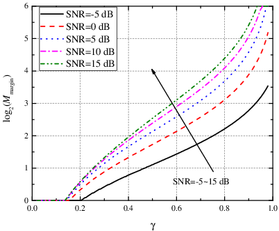
To provide a more intuitive demonstration on the relation between $\gamma$ and $M_{\text{margin}}$, in Fig. 2 we depict $M_{\text{margin}}$ as a function of $\gamma$ with various $N_{\text{0}}$. Note that we have set $b_{\text{max}}$ to be $6$. Besides, in order to better present the results, we have relaxed the requirement that $M=2^{b}$ and assume $M$ can be chosen continuously from $1$ to $2^{b_{\text{max}}}$.

As can be seen from Fig. 2, basically $M_{\text{margin}}$ becomes larger than $1$ when $\gamma$ is higher than $0.2$. More importantly, it is observed that $M_{\text{margin}}$ increases monotonically with $\gamma$. This is because, as the path gains decay slower, the more available spatial paths there will be.

We begin by demonstrating the tightness of our SE approximation $I_{\text{SPIM}}$, i.e. (12), with respect to the real MI $I(\mathbf{y};\mathbf{x},\mathbf{B}_{i})$. We denote the real MI term as “simulation”, while $I_{\text{SPIM}}$ as “theoretic” in the following figures. Note that here $\text{SNR}\triangleq N_{0}^{-1}$. The simulations are conducted with respect to “imbalanced” and “balanced” channel conditions, i.e. $(w_{1},w_{2})=(0.9,0.1)$ and $(w_{1},w_{2})=(0.6,0.4)$, respectively.

As can be seen from Fig. 3 and Fig. 4, the theoretic MI is shown to provide a relatively accurate approximation to the simulation results of MI. More importantly, in the region of high SNR (approximately over $2$ dB), the theoretic MI approximation is almost the same as its true value, which therefore justifies our usage of $I_{\text{SPIM}}$ in (12) to quantify the SE performance of SPIM-mmWave system.

Comparing $I_{\text{SPIM}}$ against $I_{\text{mmWave}}$, it can be seen that when the channel suffers from an imbalanced condition, e.g. $(w_{1},w_{2})=(0.9,0.1)$, the usage of SPIM-mmWave only leads to decreasing the achievable SE. Based on Fig. 3, SPIM-mmWave is outperformed by conventional mmWave MIMO by nearly $0.8$ bits/s/Hz. However, when the channel condition is relatively balanced, i.e. $w_{1}/w_{2}=3/2$, as in Fig. 4, the proposed SPIM-mmWave system is capable of achieving higher SE performance than conventional mmWave MIMOs. In the high-SNR region, an SE improvement of approximately $0.6$ bits/s/Hz is achieved by SPIM-mmWave, according to Fig. 4.

As can be seen from Theorem 1, the performance improvement of SPIM-mmWave relies heavily on the ratio $w_{1}/w_{2}$. In order to better illustrate the performance improvement as a function of $w_{1}/w_{2}$, we depict the SE yielded by SPIM-mmWave MIMO system (simulation-based MI as well as theoretic approximation $I_{\text{SPIM}}$) and conventional mmWave MIMO system as a function of $w_{1}\in[0,1]$ in Fig. 5, under the constraint that $w_{1}+w_{2}=1$.

According to Fig. 5, the simulation results and theoretic approximation of $I_{\text{SPIM}}$ agrees very well to each other. More importantly, it is observed that SPIM-mmWave outperforms conventional ones when $w_{1}\leq 0.8$ (i.e. $w_{1}\leq 4w_{2}$, since $w_{1}+w_{2}=1$), and is outperformed by conventional ones when $w_{1}>0.8$. This is in accordance to our asymptotic analysis of Theorem 1, thus proving the accuracy of our theoretic derivations.

Furthermore, we increase $N_{0}$ from $0.1$ to $1.0$ and depict the corresponding curves in Fig. 6. As can be observed from the figure, with the increase of $N_{0}$, the “conversion point” of $w_{1}$ becomes lower than $0.8$. As a matter of fact, SPIM-mmWave maintains its performance superiority only when $w_{1}\leq 0.76$, i.e. the performance advantage of SPIM-mmWave can be deteriorated by the increasing of noise. However the overall conclusion is not changed qualitatively, that is, SPIM-mmWave is preferred when the non-LoS channel components are non-negligible.

Finally, we look into the performance of conventional mmWave and SPIM-mmWave MIMO systems with various $\gamma$ and $M$, where $\gamma$ represents an exponential decaying factor among the path gains, as defined in (20). According to Fig. 7, under the influence of $\gamma$, the channel gains decay more slowly with the increase of $\gamma$ from $0$ to $1$. With the increase of $\gamma$, the application of SPIM-mmWave MIMO system with higher value of $M$ is preferred with respect to maximizing the achievable SE. For example, when $\gamma>0.75$, SPIM-mmWave with $M=8$ is the optimal selection, while $M=1$ (i.e. conventional mmWave) is the optimal selection only when $\gamma<0.25$.

Besides, it is also observed that the simulation and theoretic results of $I_{\text{SPIM}}$ match each other relatively close, although some deviations still present when $M$ is large. More importantly, we have also marked the three $\gamma$ values that is calculated based on (21), i.e. the minimum $\gamma$ value above which a SPIM-mmWave system with $M$ spatial paths outperforms conventional mmWave, which should satisfy the following equation,

and we denote the $\gamma$ satisfying the above equation by $\gamma(M)$ for convenience. Although $\gamma(M)$ lacks a closed-form solution, we can still numerically estimate it via Newton’s method. The calculation results are $\gamma(2)\approx 0.258$, $\gamma(4)\approx 0.425$ and $\gamma(8)\approx 0.620$. As can be seen by Fig. 7, the estimated $\gamma(M)$ agrees very well with the simulation results, which therefore proves the accuracy of our analysis.

References

- [1] S. Rangan, T. S. Rappaport, and E. Erkip, “Millimeter-wave cellular wireless networks: Potentials and challenges,” Proc. IEEE, vol. 102, no. 3, pp. 366-385, Mar. 2014.
- [2] T. S. Rappaport, J. N. Murdock, and F. Gutierrez, “State of the art in 60-GHz integrated circuits and systems for wireless communications,” Proc. IEEE, vol. 99, no. 8, pp. 1390-1436, Aug. 2011.
- [3] S. Han, C.-L. I, Z. Xu, and C. Rowell, “Large-scale antenna systems with hybrid analog and digital beamforming for millimeter wave 5G,” IEEE Commun. Mag., vol. 53, no. 1, pp. 186-194, Jan. 2015.
- [4] A. Alkhateeb, J. Mo, N. González-Prelcic, and R. Heath, “MIMO precoding and combining solutions for millimeter-wave systems,” IEEE Commun. Mag., vol. 52, no. 12, pp. 122-131, Dec. 2014.
- [5] R. Mesleh, H. Haas, S. Sinanovic, C. Ahn, and S. Yun, “Spatial modulation,” IEEE Trans. Veh. Technol., vol. 57, no. 4, pp. 2228-2241, Jul. 2008.
- [6] M. Di Renzo, H. Haas, A. Ghrayeb, S. Sugiura, and L. Hanzo, “Spatial modulation for generalized MIMO: challenges, opportunities and implementation,” Proceedings of the IEEE, vol. 102, no. 1, pp. 56-103, Jan. 2014.
- [7] P. Yang, M. Di Renzo, Y. Xiao, S. Li, and L. Hanzo, “Design guidelines for spatial modulation,” IEEE Commun. Surveys & Tutorials, vol. 17, no. 1, pp. 6-26, first quarter 2015.
- [8] J. Jeganathan, A. Ghrayeb, and L. Szczecinski, “Spatial modulation: optimal detection and performance analysis,” IEEE Commun. Lett., vol. 12, no. 8, pp. 545-547, Aug. 2008.
- [9] E. Basar, “Index modulation techniques for 5G wireless networks,” IEEE Commun. Mag., vol. 54, no. 7, pp. 168-175, July 2016.
- [10] M. Wen, X. Cheng, and L. Yang, Index modulation for 5G wireless communications, Springer, 2017.
- [11] E. Basar, M. Wen, R. Mesleh, M. Renzo, Y. Xiao, and H. Haas, “Index modulation techniques for next-generation wireless networks,” IEEE Access, vol. 5, pp. 16693-16746, Aug. 2017.
- [12] M. Wen, Q. Li, E. Basar, and W. Zhang, “Generalized multiple-mode OFDM with index modulation,” IEEE Trans. Wireless Commun., vol. 17, no. 10, pp. 6531-6543, Oct. 2018.
- [13] I. Hemadeh, et al., “Multi-set space-time shift keying and space-frequency space-time shift keying for millimeter-wave communications,” IEEE Access, vol. 5, pp. 8324-8342, Dec. 2016.
- [14] I. Hemadeh, et al., “Reduced-RF-chain aided soft-decision multi-set steered space-time shift-keying for millimeter-wave communications,” IEEE Access, vol. 5, pp. 7223-7243, Apr. 2017.
- [15] N. Ishikawa, R. Rajashekar, S. Sugiura, and L. Hanzo, “Generalized-spatial-modulation-based reduced-RF-chain millimeter-wave communications,” IEEE Trans. Veh. Techn., vol. 66, no. 1, pp. 879-883, Jan. 2017.
- [16] S. Luo, et al., “Adaptive spatial modulation for uplink mmWave communication systems,” IEEE Commun. Lett., vol. 21, no. 10, pp. 2178-2181, Oct. 2017.
- [17] L. He, J. Wang, and J. Song, “On generalized spatial modulation aided mmWave MIMO: Spectral efficiency analysis and hybrid precoder design,” IEEE Trans. Wireless Commun., vol. 16, no. 11, pp. 7658-7671, Nov. 2017.
- [18] L. He, J. Wang, and J. Song, “Spatial modulation for more spatial multiplexing: RF-chain-limited generalized spatial modulation aided mmWave MIMO with hybrid precoding,” IEEE Trans. Commun., vol. 66, no. 3, pp. 986-998, Mar. 2018.
- [19] O. Ayach, S. Rajagopal, S. Abu-Surra, Z. Pi, and R. Heath, “Spatially sparse precoding in millimeter wave MIMO systems,” IEEE Trans. Wireless Commun., vol. 13, no. 3, pp. 1499-1513, Mar. 2014.
- [20] A. Alkhateeb, O. Ayach, G. Leus, and R. Heath, “Channel estimation and hybrid precoding for millimeter wave cellular systems,” IEEE J. Sel. Topics Signal Process., vol. 8, no. 5, pp. 831-846, Oct. 2014.
- [21] C.-E. Chen, “An iterative hybrid transceiver design algorithm for millimeter wave MIMO systems,” IEEE Wireless Commun. Lett., vol. 4, no. 3, pp. 285-288, June 2015.
- [22] X. Gao, L. Dai, S. Han, C.-L. I, and R. Heath, “Energy-efficient hybrid analog and digital precoding for mmWave MIMO systems with large antenna arrays,” IEEE J. Sel. Areas Commun., vol. 34, no. 4, pp. 998-1009, Apr. 2016.
- [23] S. Park, A. Alkhateeb, and R. Heath, “Dynamic subarrays for hybrid precoding in wideband mmWave MIMO systems,” IEEE Trans. Wireless Commun., vol. 16, no. 5, pp. 2907-2920, May 2017.
- [24] A. Goldsmith, S. Jafar, N. Jindal, and S. Vishwanath, “Capacity limits of MIMO channels,” IEEE J. Sel. Areas Commun., vol. 21, no. 5, pp. 684-702, June 2003.
- [25] G. Caire and S. Shamai, “On the achievable throughput of a multi-antenna Gaussian broadcast channel,” IEEE Trans. Inf. Theory, vol. 49, np. 7, pp. 1691-1706, July 2003.
- [26] Z. An, J. Wang, J. Wang, S. Huang, and J. Song, “Mutual information analysis on spatial modulation multiple antenna system,” IEEE Trans. Commun., vol. 63, no. 3, pp. 826-843, Mar. 2015.
- [27] N. Ishikawa, S. Sugiura, and L. Hanzo, “50 years of permutation, spatial and index modulation: From classic RF to visible light communications and data storage,” IEEE Commun. Surveys & Tutorials, vol. 20, no. 3, pp. 1905-1938, third quarter 2018.