Maximum Marginal Likelihood Estimation of Phase Connections in Power Distribution Systems

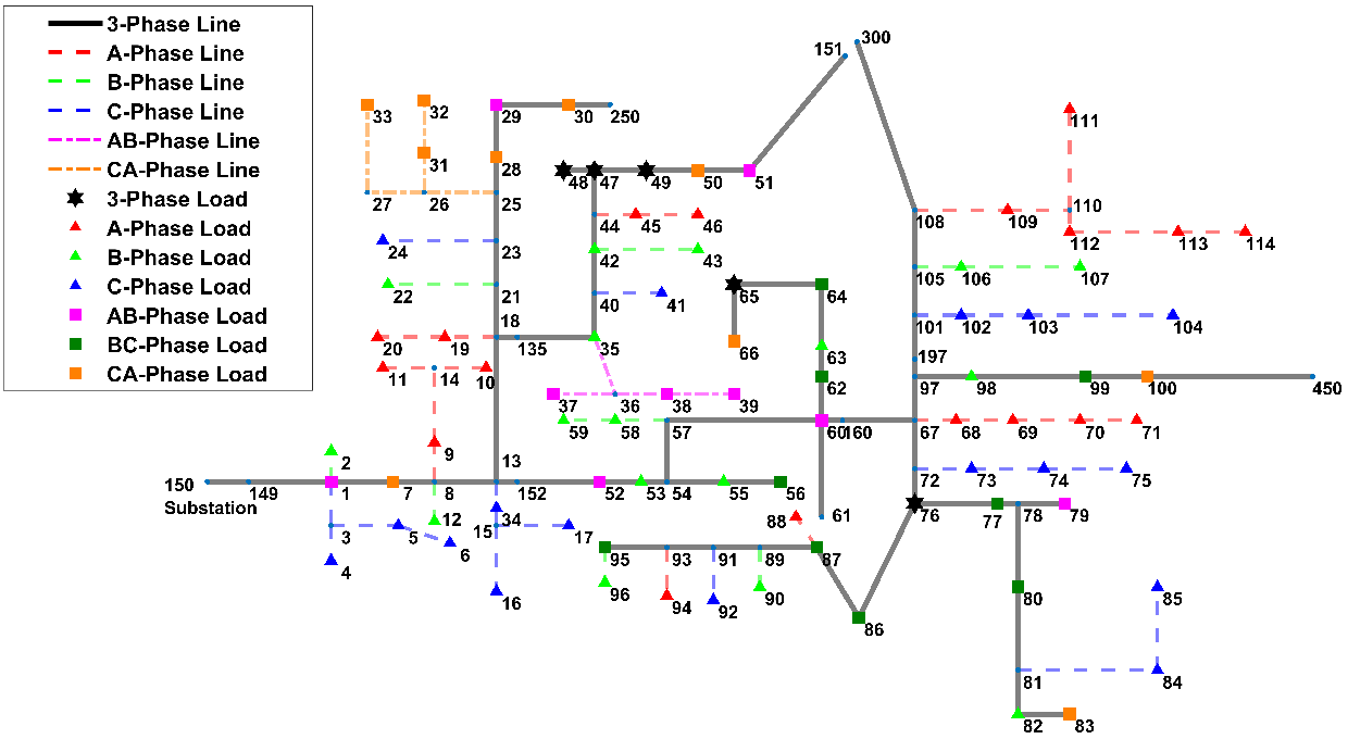
We intend to identify the type of phase connection for all loads on a distribution feeder. The distribution feeder’s three-phase primary line contains $N+1$ nodes, indexed as node $0$ to $N$, in which node $0$ is the source/substation. A load can connect to a three-phase node directly, or indirectly through a single-phase or two-phase branch (e.g., the dashed lines and dash-dot lines in Fig. 1). Note that nodes and loads are two different concepts. In the technical derivation, all variables are in per unit or radian angles unless otherwise specified.

Note that the assumptions described below are only used to prove that the correct phase connection yields the highest log likelihood value of the MLE and MMLE problem formulated in this paper. Some of these assumptions may not hold in the real world. However, the numerical study will show that our proposed algorithm still works well even when some of these assumptions no longer hold. In these cases, we can no longer guarantee that our proposed algorithm will result in $100\%$ accurate phase identification results.

The very first step of our phase identification framework is to build a three-phase power flow model for the primary feeder. To do so, we need a procedure that we call reduction, and the resulting network is called a reduced network. The reduction is simply converting any loaded single-phase or two-phase branch into an equivalent load so that the reduced network contains only three-phase lines. The details of the reduction procedure is explained in Appendix A. In the rest of the paper, we use $M$ to denote the number of loads in the reduced network and load refers to the equivalent load in the reduced network.

From the reduced primary feeder, by following [14], we can derive the linearized three-phase power flow model shown in (1), with the variables organized by phase. The linearized model ignores shunt admittance because it is very small. Numerical study results will verify that ignoring shunt admittance does not affect the phase identification accuracy.

Here $A_{11}$, $A_{12}$, $A_{21}$, and $A_{22}$ are $3(N+1)\times 3(N+1)$ matrices. $\boldsymbol{v}$, $\boldsymbol{\theta}$, $\boldsymbol{p}$, and $\boldsymbol{q}$ are the nodes’ voltage magnitude, voltage angle, and real and reactive power of three phases. $\boldsymbol{\overline{v}}=\mathbf{1}_{3(N+1)}$ and $\boldsymbol{\overline{\theta}}=[0\times\mathbf{1}^{T}_{N+1},-\frac{2\pi}{3}\times\mathbf{1}^{T}_{N+1},\frac{2\pi}{3}\times\mathbf{1}^{T}_{N+1}]^{T}$ are the flat feasible solution for the underlying nonlinear power flow model. Let $\alpha=e^{-j\frac{2\pi}{3}}$, define $\Phi\triangleq\textmd{diag}(I_{(N+1)},\ \alpha I_{(N+1)},\ \alpha^{2}I_{(N+1)})$ and define

where $Y^{ij}$ is the $(N+1)\times(N+1)$ nodal admittance matrix between phase $i$ and $j$. Then $A_{11}$, $A_{12}$, $A_{21}$, and $A_{22}$ can be calculated as $A_{11}=-A_{22}=Re(\Phi^{-1}Y\Phi)$ and $A_{12}=A_{21}=-Im(\Phi^{-1}Y\Phi)$.

It has been shown in [15] that for a connected three-phase network, $\text{rank}(Y)=3N$. Thus, $\text{rank}(A)$ is at most $6N$. For subsequent derivations, we need to transform $A$ into a nonsingular form. Following Appendix B, the transformed power flow model becomes

where $\check{A}_{mn}$ is a $3N\times 3N$ matrix obtained by removing the rows and columns corresponding to the substation node in $A_{mn}$. We denote the difference of voltage magnitudes and voltage angles between the non-substation nodes and the substation nodes as $\boldsymbol{\check{v}}$, $\boldsymbol{\check{\theta}}$. We denote the non-substation nodes’ real and reactive power as $\boldsymbol{\check{p}}$ and $\boldsymbol{\check{q}}$.

In theory, $\check{A}$ is not guaranteed to be invertible. However, for the majority of real-world distribution feeders, $\text{rank}(\check{A})=6N$. It will be shown in the numerical study section that for all IEEE distribution test feeders, $\check{A}$ has a full rank.

Solving for ${\check{v}}$ with ${\check{p}}$ and ${\check{q}}$ from (3), we have

or in condensed form as

It can be shown that $(\check{A}_{11}-\check{A}_{12}\check{A}_{22}^{-1}\check{A}_{21})$ is invertible if $\check{A}$ is invertible. Similarly, we can link $\boldsymbol{\check{\theta}}$ with $\boldsymbol{\check{p}}$ and $\boldsymbol{\check{q}}$ as

or in condensed form as

The linearized three-phase power flow models (5) and (7) are derived in terms of nodal voltages and power injections $\boldsymbol{\check{v}}$, $\boldsymbol{\check{\theta}}$, $\boldsymbol{\check{p}}$, and $\boldsymbol{\check{q}}$, which are often not directly measured by smart meters. Thus, we need to embed the smart meter measurements into these two equations. This is straightforward for single-phase and three-phase loads. For a single-phase load $m$ on node $n$, its voltage measurement $\hat{v}_{m}$ is equal to one of the three phase-to-neutral voltage magnitudes $v_{n}^{i}\ (i=a,b,c)$, which is related to $\check{v}_{n}^{i}$ in (3) via $\check{v}_{n}^{i}\triangleq v_{n}^{i}-v_{0}^{i}$, where $v_{0}^{i}$ is the source voltage magnitude in phase $i$. Similarly, a single-phase load’s power injection measurement $\hat{p}_{m}+j\hat{q}_{m}$ corresponds to the power injection of one of the three phases $\check{p}_{n}^{i}+j\check{q}_{n}^{i}$ at node $n$. For a three-phase load $m$ at node $n$, the single-phase voltage measurement $\hat{v}_{m}$ is equal to one of the three nodal voltage magnitudes $v_{n}^{i}\ (i=a,b,c)$. We can assume that the three-phase power injections $\hat{p}_{m}+j\hat{q}_{m}$ is distributed relatively evenly to three phases at node $n$. For a delta-connected two-phase load, we need the following derivations to link its measurements to the three-phase power flow model.

Let $\boldsymbol{x}\triangleq[x_{1}^{1},x_{1}^{2},x_{1}^{3},...,x_{M}^{1},x_{M}^{2},x_{M}^{3}]^{T}$ be the phase connection decision variable vector. Define $\boldsymbol{\tilde{v}}(t,\boldsymbol{x})$ as the theoretical differenced voltage measurement $\boldsymbol{\tilde{v}}(t)$ with phase connection $\boldsymbol{x}$:

Then $\boldsymbol{\tilde{v}}(t)=\boldsymbol{\tilde{v}}(t,\boldsymbol{x})+\boldsymbol{n}(t)$, where $\boldsymbol{x}$ is the phase connection decision variable vector that we need to estimate.

As stated in Section II-B, we assume that the noise $\boldsymbol{n}(t)$ is independent of $\boldsymbol{\tilde{v}}^{\text{ref}}(t)$, $\boldsymbol{\tilde{p}}(t)$, and $\boldsymbol{\tilde{q}}(t)$ and is i.i.d. Gaussian $\boldsymbol{n}(t)\sim\mathcal{N}(\mathbb{0}_{M\times 1},\Sigma_{n})$, where $\Sigma_{n}$ is an unknown underlying covariance matrix. Given these conditions, $\boldsymbol{n}(t)$ is also independent of $\boldsymbol{\tilde{v}}(t,\boldsymbol{x})$. Thus, the likelihood of observing $\{\boldsymbol{\tilde{v}}(t)\}^{T}_{t=1}$ given $\{\boldsymbol{\tilde{v}}^{\text{ref}}(t)\}^{T}_{t=1}$, $\{\boldsymbol{\tilde{p}}(t)\}^{T}_{t=1}$, and $\{\boldsymbol{\tilde{q}}(t)\}^{T}_{t=1}$ is a function of $\boldsymbol{x}$:

Taking the negative logarithm of (18), removing the constant term, and scaling by $\frac{2}{T}$, we get

It will be shown in Lemma 1 that the correct phase connection $\boldsymbol{x^{*}}$ maximizes the likelihood function (18) and minimizes $f(x)$ under two mild assumptions.

The proof of Lemma 1 can be found in Appendix E. By substituting (17) into (19), we can see that directly minimizing $f(\boldsymbol{x})$ is very difficult due to its nonlinearity and nonconvexity. Furthermore, the actual value of $\Sigma_{n}$ is unknown. To address this technical challenge, in Section IV-B, we will convert the phase identification problem into an MMLE problem and prove that the correct phase connection is also a global optimizer of the MMLE problem.

Let $\tilde{v}_{m}(t)$ be the $m$th entry of $\boldsymbol{\tilde{v}}(t)$, $\tilde{v}_{m}(t,\boldsymbol{x})$ be the $m$th entry of $\boldsymbol{\tilde{v}}(t,\boldsymbol{x})$, and $n_{m}(t)$ be the $m$th entry of $\boldsymbol{n}(t)$. The marginal likelihood of observing $\{\tilde{v}_{m}(t)\}^{T}_{t=1}$ given $\{\boldsymbol{\tilde{v}}^{\text{ref}}(t)\}^{T}_{t=1}$, $\{\boldsymbol{\tilde{p}}(t)\}^{T}_{t=1}$, and $\{\boldsymbol{\tilde{q}}(t)\}^{T}_{t=1}$ is a function of $\boldsymbol{x}$:

where $\Sigma_{n}(m,m)$ is the $m$th diagonal entry of $\Sigma_{n}$. Taking the negative logarithm of (20), removing the constant term, and scaling by $\frac{2\Sigma_{n}(m,m)}{T}$, we have

The proof of Lemma 2 can be found in Appendix F.

Directly minimizing $f_{m}(\boldsymbol{x})$ from (21) is still a difficult task. Thus, we further simplify the optimization problem by first solving three subproblems $minf_{m,i}(\boldsymbol{x}_{-m}),i\in\{1,2,3\}$. $f_{m,i}(\boldsymbol{x}_{-m})$ are defined as

where $\boldsymbol{x}_{-m}$ is a $(3M-3)\times 1$ vector containing every element in $\boldsymbol{x}$ except $x_{m}^{1}$, $x_{m}^{2}$, and $x_{m}^{3}$. Since $x_{m}^{i}=0\ \text{or}\ 1$, and $\sum_{i}x_{m}^{i}=1$, then from (22) we have:

To solve the sub-problems, we first define $\tilde{v}_{m,i}(t,\boldsymbol{x}_{-m})$ as

Substituting (17) into (24), we have

where $\tilde{v}^{\text{ref}}_{m,i}(t)$ is the entry of $\boldsymbol{\tilde{v}}^{\text{ref}}(t)$ corresponding to $x_{m}^{i}$, $\hat{K}_{m,i}$ and $\hat{L}_{m,i}$ are the row vectors of $\hat{K}$ and $\hat{L}$ corresponding to $x_{m}^{i}$.

Define an $M\times 3M$ matrix $\mathfrak{D}$ as:

Then matrix $X$ can be expressed by decision vector $\boldsymbol{x}$ as $X=\mathfrak{D}\ \textmd{diag}(\boldsymbol{x})$. Thus, we can simplify the second term on the right-hand-side (RHS) of (25) as

where $\boldsymbol{\zeta}_{m,i}(t)\triangleq\textmd{diag}(\hat{K}_{m,i})\ \mathfrak{D}^{T}\ \boldsymbol{\tilde{p}}(t)$. Similarly, simplify the third term on the RHS of (25) as

where $\boldsymbol{\xi}_{m,i}(t)\triangleq\textmd{diag}(\hat{L}_{m,i})\ \mathfrak{D}^{T}\ \boldsymbol{\tilde{q}}(t)$.

Substituting (27) and (28) into equation (25), we have

Where $\boldsymbol{\psi}_{m,i}(t)\triangleq\boldsymbol{\zeta}_{m,i}(t)+\boldsymbol{\xi}_{m,i}(t)$. $\boldsymbol{\varphi}_{m,i}(t)$ is a vector containing all the elements in $\boldsymbol{\psi}_{m,i}(t)$ except the three elements corresponding to $x_{m}^{1}$, $x_{m}^{2}$, and $x_{m}^{3}$. $\eta_{m,i}(t)$ is the element in $\boldsymbol{\psi}_{m,i}(t)$ corresponding to $x_{m}^{i}$. In the last line of (29), $v^{\text{tot}}_{m,i}(t)$ is defined as $v^{\text{tot}}_{m,i}(t)\triangleq\tilde{v}_{m}(t)-\tilde{v}^{\text{ref}}_{m,i}(t)-\eta_{m,i}(t)$.

Note that our proposed phase identification method still works even if there is a topology change in the primary feeder. If such topology change occurs at time $t_{c}$, then we can simply update $v^{\text{tot}}_{m,i}(t)$ and $\boldsymbol{\varphi}_{m,i}(t)$ in (29) according to the new primary feeder topology.

With (29), the function $f_{m,i}(\boldsymbol{x}_{-m})$ can be transformed into

Now each MMLE sub-problem in (23) can be formulated as

This is a binary least-square problem. To solve it efficiently, we can further relax the problem by replacing the binary constraint by its convex hull. Now the problem is equivalent to convex quadratic programming, which can be solved in polynomial time [16]. The continuous solution of $\boldsymbol{x}_{-m}$ in the convex hull can then be rounded to binary values as follows: for each load $k\neq m$, round $x_{k}^{j}$ to $1$ if it is the largest among $x_{k}^{1}$, $x_{k}^{2}$, and $x_{k}^{3}$, and round the other two variables to 0.

Our proposed MMLE-based phase identification algorithm is summarized in Algorithm 1 and explained as follows. From step 1 to 6, we solve $M$ MMLE problems, each of which contains three binary least-square sub-problems. Step 3 solves the sub-problems of MMLE based on (31). Based on (23), step 5 solves the $m$th MMLE problem by finding which of the three $\boldsymbol{x}^{{\dagger}}_{-m,i}\ (i=1,2,3)$ minimizes $f_{m}(\boldsymbol{x})$. The chosen $\boldsymbol{x}^{{\dagger}}_{-m,i}$, combined with the corresponding $x_{m}^{i}=1$ and $x_{m}^{j}=0$ ($j\neq i$), forms the $3M\times 1$ solution $\boldsymbol{x^{{\dagger}}}_{m}$ of the $mth$ MMLE problem. The $M$ sets of $\boldsymbol{x^{{\dagger}}}_{m}$ may not be all correct due to the limited number of measurements and measurement noise. Thus, in step 7, we design two approaches to integrate $M$ sets of $\boldsymbol{x^{{\dagger}}}_{m}$ into two phase identification solutions:

1. 1.

   Target-only Approach. The phase connection of each load $m$ is the corresponding connection shown in the $m$th solution $\boldsymbol{x^{{\dagger}}}_{m}$.

2. 2.

   Voting Approach. For a single-phase or two-phase load $m$, the phase connection is the corresponding phase connection that receives the most votes in the $M$ sets of $\boldsymbol{x^{{\dagger}}}_{m}$. For a three-phase load $m$, the phase connection is still determined by the target-only approach.

In step 8, we calculate $\sum_{m=1}^{M}f_{m}(\boldsymbol{x})$ based on the phase identification solution of both the target-only and the voting approaches. The final phase identification solution is the one that has the lower sum of square error.

The performance of our proposed MMLE-based algorithm is evaluated using the IEEE 37-bus, 123-bus, and 342-bus test circuits. The results will show that the proposed algorithm works well for distribution networks with either tree structured feeders (37-bus and 123-bus) or heavily meshed primary feeders (342-bus). To make the task more difficult, we modify the test feeders to include all possible phase connection types (single-phase, two-phase, and three-phase). The number of loads by phase connection type is summarized in Table II. Fig. 1 illustrates the schematic of the 123-bus circuit.

The hourly average real power consumption measurements from smart meters of a distribution feeder managed by FortisBC are used in test feeders. The length of the real power consumption time series is 2160, which represents 90 days of hourly smart meter measurements. The reactive power time series are generated by randomly sampling power factors from a uniform distribution $\mathcal{U}(0.9,1)$ to represent lagging loads. The peak loads for the three IEEE test circuits are 2.4 MW, 4 MW, and 43 MW. The power flows of the test circuits are simulated using OpenDSS. All smart meter measurements contain noise that follows zero-mean Gaussian distributions with three-sigma deviation matching 0.1% to 0.2% of the nominal values. The 0.1 and 0.2 accuracy class smart meters established in ANSI C12.20-2015 are typical in real-world implementations. To make the phase identification task even more challenging, we assume that older generations of smart meters are adopted. That is to say, after adding measurement noise, the voltage measurements are rounded to the nearest 1 V for primary line loads and 0.1 V for secondary loads. The real and reactive power measurements are rounded to the nearest 0.1 kW or 0.1 kVAr. The relaxed optimization problems in equation (31) are solved using CPLEX on a DELL workstation with 3.3 GHz Intel Xeon CPU and 16 GB of RAM.

Before presenting the main numerical results, we first verify the Gaussianity assumption for the noise term $\boldsymbol{n}(t)$ in equation (16). The Kolmogorov-Smirnov test is used to verify the Gaussianity assumption. With a significance level of 5%, the noise terms for all loads pass the test except 9 loads at 0.1% meter accuracy level and 1 load at 0.2% meter accuracy level in the 342-bus circuit. By checking the normalized auto-correlations of $n(t)$, we found the noise to be uncorrelated over time. For Gaussian random variables, this indicates independence over time.

References

- [1] W. S. Bierer, “Long range phasing voltmeter,” Oct. 5 2010, US Patent 7,808,228.
- [2] M. H. Wen, R. Arghandeh, A. von Meier, K. Poolla, and V. O. Li, “Phase identification in distribution networks with micro-synchrophasors,” in 2015 IEEE Power & Energy Society General Meeting. IEEE, Jul. 2015, pp. 1–5.
- [3] Y. Liao, Y. Weng, G. Liu, Z. Zhang, C. W. Tan, and R. Rajagopal, “Unbalanced three-phase distribution grid topology estimation and bus phase identification,” arXiv preprint arXiv:1809.07192 [cs.SY], Sep. 2018.
- [4] V. D. Krsman and A. T. Sarić, “Verification and estimation of phase connectivity and power injections in distribution network,” Electric Power Systems Research, vol. 143, pp. 281–291, Feb. 2017.
- [5] M. Dilek, “Integrated design of electrical distribution systems: Phase balancing and phase prediction case studies,” Ph.D. dissertation, Virginia Polytechnic Institute and State University, 2001.
- [6] P. Kumar, V. Arya, D. A. Bowden, and L. Kohrmann, “Leveraging DERs to improve the inference of distribution network topology,” in 2017 IEEE International Conference on Smart Grid Communications (SmartGridComm). IEEE, Oct. 2017, pp. 52–57.
- [7] S. J. Pappu, N. Bhatt, R. Pasumarthy, and A. Rajeswaran, “Identifying topology of low voltage distribution networks based on smart meter data,” IEEE Transactions on Smart Grid, vol. 9, no. 5, pp. 5113–5122, Mar. 2018.
- [8] T. A. Short, “Advanced metering for phase identification, transformer identification, and secondary modeling,” IEEE Transactions on Smart Grid, vol. 4, no. 2, pp. 651–658, Jun. 2013.
- [9] W. Luan, J. Peng, M. Maras, J. Lo, and B. Harapnuk, “Smart meter data analytics for distribution network connectivity verification,” IEEE Transactions on Smart Grid, vol. 6, no. 4, pp. 1964–1971, Jul. 2015.
- [10] M. Xu, R. Li, and F. Li, “Phase identification with incomplete data,” IEEE Transactions on Smart Grid, vol. 9, no. 4, pp. 2777–2785, Jul. 2018.
- [11] W. Wang, N. Yu, B. Foggo, J. Davis, and J. Li, “Phase identification in electric power distribution systems by clustering of smart meter data,” in 2016 15th IEEE International Conference on Machine Learning and Applications (ICMLA). IEEE, Dec. 2016, pp. 259–265.
- [12] W. Wang and N. Yu, “Advanced metering infrastructure data driven phase identification in smart grid,” in The Second International Conference on Green Communications, Computing and Technologies, Sep. 2017, pp. 16–23.
- [13] F. Olivier, A. Sutera, P. Geurts, R. Fonteneau, and D. Ernst, “Phase identification of smart meters by clustering voltage measurements,” in 2018 Power Systems Computation Conference (PSCC). IEEE, Jun. 2018, pp. 1–8.
- [14] S. Bolognani and F. Dörfler, “Fast power system analysis via implicit linearization of the power flow manifold,” in 2015 53rd Annual Allerton Conference on Communication, Control, and Computing (Allerton). IEEE, Sep. 2015, pp. 402–409.
- [15] A. M. Kettner and M. Paolone, “On the properties of the compound nodal admittance matrix of polyphase power systems,” IEEE Transactions on Power Systems, vol. 34, no. 1, pp. 444–453, Aug. 2019.
- [16] S. A. Vavasis, Complexity theory: Quadratic programming. Boston, MA: Springer US, 2001, pp. 304–307. [Online]. Available: {https://doi.org/10.1007/0-306-48332-7_65}
- [17] W. H. Greene, Econometric Analysis, 7th ed. Pearson, 2011.
Appendix A Simplification of Single-Phase and Two-Phase Branches
To convert loaded single-phase and two-phase branches into a load directly connected to the primary feeder, we need to estimate each branch’s equivalent power injection and voltage magnitude. In other words, given the line impedances of single-phase and two-phase branches, the voltage magnitudes and power injections of the loads, we need to calculate the equivalent power injection and voltage magnitude on the primary feeder. The conversion of single-phase and two-phase branches is carried out separately below.
A-1 Simplification of a Single-Phase Line
Suppose there is a single-phase line with impedance serving a load with power injection and voltage magnitude . It is assumed that the power injection and the voltage magnitude are given. Thus, the current injection magnitude and power factor angle can be calculated. Then, at the upstream port of the primary feeder, the single-phase line’s equivalent voltage magnitude is and the equivalent power injection is .
A-2 Simplification of a Two-Phase Line
For a two-phase line serving a load, the voltage drop along the line section can be described by