Tensors for tending to tensions in $\tau$ decaysPreprint: TIFR/TH/19-3

Decays of $\tau$ leptons provide a laboratory for precision tests of the Standard Model (SM) of particle physics Davier:2005xq; Pich:2013lsa. Leptonic $\tau$ decays are crucial for testing lepton flavor universality and searching for lepton flavor violating decays Amhis:2016xyh; Tanabashi:2018oca. Hadronic $\tau$ decays offer us the opportunity to probe strong interactions in a variety of ways. Since the mass of $\tau$ is fairly above the QCD scale, we can use perturbative results derived in the effective field theory framework. These decays have been used to extract fundamental parameters of SM, such as the strong coupling constant $\alpha_{s}$ Braaten:1991qm; Davier:2008sk; Boito:2014sta; Pich:2016bdg. As $\tau$ is massive enough to decay to strange mesons, these decays have also been used to determine the strange quark mass and the $V_{us}$ element of the Cabibbo–Kobayashi–Maskawa (CKM) matrix Gamiz:2002nu; Gamiz:2004ar; Baikov:2004tk.

Consistency across various measurements of the above parameters vouches for the success of SM. However further precision measurements of $\tau$ decays can uncover hints of new physics (NP) beyond SM, through deviations from SM predictions. In this work, we take a critical look at two such long-standing anomalies in hadronic $\tau$ decays:

• •

  The determination of $V_{us}$ from inclusive $\tau$ decays to final states including the strange quark. The value extracted from inclusive decays Amhis:2016xyh,

  $$|V_{us}|^{\tau,\text{in}}=0.2186\pm 0.0021\;,$$

  (1)

  shows a striking $3.1\sigma$ deviation from the CKM unitarity prediction,

  $$|V_{us}|^{\text{uni}}=0.22582\pm 0.00089\;.$$

  (2)

• •

  The CP asymmetry in $\tau\rightarrow K_{s}\pi\nu_{\tau}$ is calculated in SM to be Bigi:2005ts; Grossman:2011zk

  $$A_{CP}^{\tau,\,{\rm SM}}=(0.33\pm 0.01)\%\;.$$

  (3)

  However the asymmetry measured by the BaBar collaboration BABAR:2011aa,

  $$A_{CP}^{\tau,\,\text{exp}}=(-0.36\pm 0.23\pm 0.11)\%\;,$$

  (4)

  is $2.8\sigma$ below the SM prediction.

Various attempts have been made in the literature to reconcile the $V_{us}$ anomaly within SM. Proposals range from inadequate theoretical understanding of $\tau$ spectral functions Boyle:2018ilm; Hudspith:2017vew to possible mis-measurements of some exclusive $\tau$ decay channels Antonelli:2013usa. (The measurement of inclusive $\tau\to s$ decays is through the summation over all exclusive decay modes with an odd numbers of kaons Amhis:2016xyh in the final state.) It is, however, not possible to account for the discrepancy in $CP$ asymmetry within SM Devi:2013gya; Dhargyal:2016kwp; Cirigliano:2017tqn. It was pointed out in Ref. Devi:2013gya that scalar NP operators cannot generate new $CP$ asymmetry while tensors can. However Ref. Cirigliano:2017tqn claimed that a demand of gauge invariance brings the tensor operator in conflict with the measurement of neutron electric dipole moment (EDM). This claim has recently been repeated in Ref. Rendon:2019awg.

In this Letter, we address both the above $\tau$ anomalies with a single source of NP in the effective field theory (EFT), and provide an explicit renormalizable model. The essential requirements we impose are $(i)$ no effect on $V_{us}$ extraction from exclusive $\tau$ decays, which is consistent with SM within $\sim 1\sigma$, $(ii)$ manifest electroweak (EW) gauge invariance.

To comply with the the first requirement, the new operator $\mathcal{O}_{\text{NP}}$ should be such that

This condition is satisfied automatically if $\mathcal{O}_{\text{NP}}^{\text{had}}$, the hadronic part of the NP operator, has a tensorial structure. This is because $\langle K|\bar{q}\ \sigma_{\mu\nu}\gamma_{5}\ q^{\prime}|0\rangle=0$ for any flavors $q,q^{\prime}$, due to the antisymmetry of the Lorentz structure of the operator. Note that the symmetry argument would not be valid if the outgoing state were to involve more than one hadron. Therefore, by choosing the flavor structure of $\mathcal{O}_{\text{NP}}^{\text{had}}$ appropriately, one can contribute to inclusive $\tau$ decays. Thus a suitable choice of $\mathcal{O}_{\text{NP}}$ that accounts for the $V_{us}$ discrepancy would be the tensor operator $\left(\bar{s}\sigma_{\mu\nu}u\right)\left(\ \bar{\nu}_{\tau}\sigma^{\mu\nu}\tau\right)$.

Remarkably, the same operator can also contribute to the $CP$ asymmetry in $\tau\rightarrow K_{s}\pi\nu_{\tau}$ Devi:2013gya. Therefore, it may be possible to reconcile both these anomalies by a unified explanation. On the other hand, according to Ref. Cirigliano:2017tqn, a demand of EW gauge invariance necessarily gives rise to an additional operator $\left(\bar{u}_{L}\sigma_{\mu\nu}u_{R}\right)\left(\tau_{L}\sigma^{\mu\nu}\tau_{R}\right)$, which is strongly constrained from neutron EDM measurements. Consequently, there appears to be a “no-go” for the explanation of the $CP$ anomaly.

In this Letter, we argue that the no-go theorem sketched in Ref. Cirigliano:2017tqn only pertains to a specific way of imposing gauge invariance. We demonstrate that there exists at least one class of manifestly gauge invariant operators that can accommodate both anomalies in $\tau$ decays and yet is safe from neutron EDM constraints. As a concrete example, we propose a renormalizable flavor model (detailed later in this article) which appends to SM the following gauge invariant effective tensor operator after integrating out all beyond-SM degrees of freedom:

where $\Lambda$ represents the scale of the operator, defined such that $\left|\mathcal{K}\right|=1$. In our model, after electroweak symmetry breaking (EWSB), Eq. (6) yields a single operator where all the fields are written in the mass basis:

We have used

with $v=246~\text{GeV}$ is the EWSB scale, and $G_{F}$ is the Fermi constant. (Note that the factor of $V_{us}$ is used in the normalization of $C_{T}$, only to simplify further calculations.) This corresponds to a 4-fermion interaction with effective coupling strength $\mathcal{K}v^{2}/2\Lambda^{4}$. The NP coupling via the Higgs doublet in Eq. (6) ensures that the dangerous operator that would have contributed to the neutron EDM is not generated.

Before going to the details of the renormalizable model, we now quantitatively explore our solutions to the above two $\tau$ anomalies, including constraints from other relevant measurements. In SM, $\tau$ decays to strange and non-strange hadrons proceed via the standard 4-fermi interaction,

Let us first explore the extraction of $V_{us}$ from inclusive decay channels. In this extraction, strange and non-strange spectral functions of $\tau$ are used along with very precisely determined value of $V_{ud}$. The relevant quantity is Braaten:1991qm

where $R_{\tau,\text{ns}}$ and $R_{\tau,\text{s}}$ are the partial widths defined as

Here $X_{\text{ns}(\text{s})}$ represents the final state with even (odd) strangeness. The quantity $\delta R_{\tau}$, which vanishes in the perturbative and massless quark limit, encodes the corrections due to finite quark masses and non-perturbative effects. Using QCD sum rules and operator product expansion (OPE) Shifman:1978bx; Shifman:1978by; Craigie:1981jx, this factor is theoretically calculated in SM to be Gamiz:2004ar; Gamiz:2006xx

Using this theoretical input and experimentally determined values of $R_{\tau,\text{s}}$, $R_{\tau,\text{ns}}$, and $V_{ud}$ Amhis:2016xyh, the CKM element $V_{us}$ is extracted using Eq (10), and is found to be nearly $3.1\,\sigma$ Amhis:2016xyh below the CKM unitarity prediction.

Now we calculate the effect of our NP on this extraction. We expect that the tensor operator will modify $R_{\tau,\text{s}}$, thereby changing the theoretical value of $\delta R_{\tau}$. The effect of this operator on the inclusive mode can be calculated using QCD sum rules and OPE Craigie:1981jx; Cata:2007ns. We parametrize the corrections due to NP as

and find

where $\bar{q}q\equiv(\bar{u}u+\bar{s}s)/2$. In deriving the above, we have ignored higher order correction to OPE due to quark masses, gluon condensates, higher order corrections in $\alpha_{s}$, and duality violation Chibisov:1996wf; Shifman:2000jv; Cata:2005zj effects.

The first term in Eq. (14) arises from the interference of the SM operator in Eq. (9) with the tensor operator that we introduced in Eq. (7), and therefore is linear in $C_{T}$. The second term, quadratic in $C_{T}$, comes from the tensor-tensor correlator. We briefly sketch the derivation of Eq. (14), and specially the estimation of the tensor-tensor correlator, in Appendix A.

Let us turn towards the other anomaly, namely, the $CP$ asymmetry in $\tau\rightarrow K_{s}\pi\nu_{\tau}$ decays:

In SM, the source of this asymmetry is indirect $CP$ violation due to $K-\overline{K}$ mixing in the final state Bigi:2005ts. After the initial inconclusive null results from CLEO Bonvicini:2001xz and Belle Bischofberger:2011pw, the BaBar collaboration has measured this $CP$ asymmetry at the PEP-II asymmetric-energy $e^{+}$-$e^{-}$ collider at SLAC BABAR:2011aa.

The events in the signal channel $\tau\rightarrow\pi K^{0}_{S}\nu_{\tau}$(C1) at BaBar also receive significant contamination from the two background channels, $\tau\rightarrow KK^{0}_{S}\nu_{\tau}$(C2) and $\tau\rightarrow\pi K^{0}\bar{K}^{0}\nu_{\tau}$(C3). Therefore, the actual asymmetry measured is BABAR:2011aa

Here $A_{1}$, $A_{2}$, $A_{3}$ are $CP$ asymmetries in the channels C1, C2, C3, respectively, while $f_{1},f_{2},f_{3}$ are the corresponding sample fractions. Note that the above $CP$ asymmetries measured in the experiment are also affected by the $K_{S}\rightarrow\pi^{+}\pi^{-}$ decay time dependence of the event selection efficiency Grossman:2011zk. As argued by BaBar, this results in a multiplicative correction factor such that BABAR:2011aa

In SM, $A_{1}=-A_{2}$, and $A_{3}=0$. Using these relations and the measurement $\mathcal{A}^{\text{exp}}=(-0.27\pm 0.18\pm 0.08)\%$, BaBar extracted $A_{1}^{\text{exp}}=(-0.36\pm 0.23\pm 0.11)\%$. The corresponding SM prediction is $A_{1}^{\text{SM}}=(+0.36\pm 0.01)\%$. This is the $2.8\,\sigma$ discrepancy in the $CP$ asymmetry in $\tau$ decays.

While introducing NP, a very important point needs to be considered which has been overlooked in previous analyses Devi:2013gya; Dhargyal:2016kwp; Cirigliano:2017tqn. The extraction of $A_{1}$ from $\mathcal{A}$ as done by BaBar, while valid in SM, fails in the presence of NP. This is because in general, $A_{1}\neq-A_{2}$. Therefore the comparison of predictions in the presence of NP needs to be done with the measured quantity $\mathcal{A}$, and not with $A_{1}$. The NP operator as introduced by us in Eq. (7) affects only the channel C1. Therefore

While $A_{1}^{\text{SM}}$ is positive, the direct CP violation arising from interference of the $V$–$A$ operator in Eq. (9) and the tensor operator in Eq. (7) can lead to a negative $A_{1}^{\text{NP}}$. This would move the value of $A_{1}$, and hence the value of $\mathcal{A}$, closer to the measurement.

In the presence of both, indirect $CP$ violation from SM ($A^{\tau,\text{SM}}_{CP}$) and direct $CP$ violation from NP ($A^{\tau,\text{NP}}_{CP}$), the net $CP$ asymmetry may be written in the form Devi:2013gya

The value of $A^{\tau,\text{NP}}_{CP}$ may be expressed in terms of the vector and tensor form factors $f_{+}(s)$ and $B_{T}(s)$, defined through

where $s\equiv(p_{\pi}+p_{K})^{2}$. The asymmetry, as may be obtained from the differential decay rate Devi:2013gya; Cirigliano:2017tqn (see Appendix B), is

where

Here the denominator $\Gamma_{\tau}\text{BR}(\tau\rightarrow K_{s}\pi\nu_{\tau})$ is the average decay width of $\tau^{\pm}\rightarrow K_{s}\pi^{\pm}{\nu_{\tau}}$. In the integral $\mathcal{I}$, we denote $s_{\pi K}=(m_{\pi}+m_{K})^{2}$, and $\kappa(s)$ is defined as

where $\lambda(a,b,c)=a^{2}+b^{2}+c^{2}-2(ab+bc+ca)$, and $S_{\text{EW}}=1.0194$ Marciano:1988vm; Braaten:1990ef is the EW correction factor. Here $\delta_{+}(s)$ and $\delta_{T}(s)$ are the phases of the form factors $f_{+}(s)$ and $B_{T}(s)$, respectively.

In the decay $\tau\to K_{s}\pi\nu_{\tau}$, the relevant form factors are dominated by the $K^{*}(892)$ resonance in the elastic limit and $K^{*}(1410)$ in the inelastic region. Both these resonances can have contributions from $f_{+}(s)$ as well as $B_{T}(s)$, with $\delta_{+}(s)=\delta_{T}(s)$ in the elastic limit as guaranteed by Watson’s final-state theorem PhysRev.95.228. Therefore only the inelastic region contributes to $\mathcal{I}$, and hence to the $CP$ asymmetry.

The value of $\mathcal{I}$ is highly uncertain, mainly due to lack of information on $B_{T}(s)$. Assuming only SM, the value of $f_{+}(s)$ is obtained by fitting to a superposition of Breit-Wigner (BW) functions, Epifanov:2007rf or by using the dispersive parametrization Boito:2008fq; Boito:2010me; Antonelli:2013usa. In the context of NP, Ref. Cirigliano:2017tqn uses simplified “Omnès function” forms Omnes:1958hv for the magnitudes of $f_{+}(s)$ and $B_{T}(s)$, with the phase difference $\delta_{+}(s)-\delta_{T}(s)$ proportional to the BW phase of $K^{\ast}(1410)$. The constraint $|A^{\tau,NP}_{CP}|\lesssim 0.03\,|\text{Im}~C_{T}|$, obtained therein, is crucially dependent on the value of $\delta_{+}(s)$ used, and on the assumed relation $\delta_{T}(s)=-\delta_{+}(s)$ in the inelastic region, which has no strong theoretical motivation. Here we employ a more general treatment, with the same Omnès forms for $|f_{+}(s)|$ and $|B_{T}(s)|$, but with

which is automatically consistent with Watson’s final-state theorem PhysRev.95.228. The free real parameter $\alpha$ acts as a proxy for our ignorance about $\mathcal{I}$, and hence we can study the dependence of NP constraints for different values of $\alpha$ (hence for different values of $\mathcal{I}$). We have taken $f_{+}(0)|V_{us}|=0.2166(5)$ Antonelli:2009ws, whereas $B_{T}(0)/f_{+}(0)=0.676(27)$ Baum:2011rm from lattice calculations.

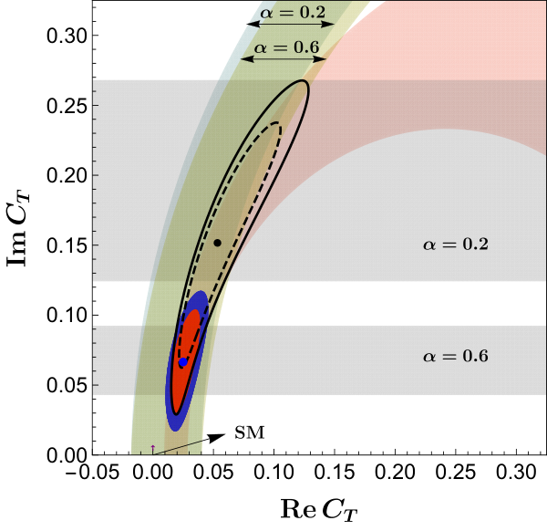
We show our numerical results of the constraints on real and imaginary parts of $C_{T}$ in Fig. 1. The $1\sigma$ allowed regions ($1$ d.o.f, $\Delta\chi^{2}\leq 1$) explaining $A_{\text{CP}}^{\tau}$, for two representative $\alpha$ values $(\alpha=0.2,0.6)$, are shown with horizontal grey bands. Note that all our results are invariant under $\{\alpha\rightarrow-\alpha,~\text{Im}(C_{T})\rightarrow-\text{Im}(C_{T})\}$. The value $\alpha=0.2$ approximately corresponds to the phase choices in Ref. Cirigliano:2017tqn.

The NP introduced will also affect the decay rates of $\tau\to K_{s}\pi\nu$ and $\tau\to K^{-}\pi^{0}\nu$. Since the theoretical predictions for these quantities are isospin-related, and hence completely correlated Antonelli:2013usa, we only use the branching ratio (BR) measurement for $\tau\to\bar{K}^{0}\pi\nu=0.8386\pm 0.0141$ Amhis:2016xyh. The SM value of the BR is taken from Antonelli:2013usa. The $1\sigma$ constraints ($2$ d.o.f, $\Delta\chi^{2}\leq 2.3$) in the $C_{T}$ plane are shown in Fig. 1 for $\alpha=0.2~\text{and }0.6$, with light blue and light green bands, respectively.

Fig. 1 also shows the $1\sigma$ ($2$ d.o.f, $\Delta\chi^{2}\leq 2.3$) allowed regions explaining the $V_{us}$ anomaly from inclusive $\tau$ decays. The values of quark condensates are taken from Ref. McNeile:2012xh and of other relevant quantities from Refs. Amhis:2016xyh; Tanabashi:2018oca. We have included $10\%$ theoretical errors in the coefficients of the two terms in Eq. (14).

We finally show the combined results from $A_{CP}^{\tau}$, the BR of $\tau\to K_{s}\pi\nu$, and the $V_{us}$ anomaly, for $\alpha=0.2,0.6$. Clearly the range of preferred values of NP parameters depends of $\alpha$. For example, for $\alpha=0.6$, the best-fit value of $\text{Im}(C_{T})$ is $0.067$, which is substantially lower than the required value implied in Ref. Cirigliano:2017tqn. Note that this best-fit point has $|C_{T}|\approx 0.072$, which corresponds to $\Lambda\sim 580\,\text{GeV}$. However, a reliable prediction for $\mathcal{I}$ is needed to pin down the scale of NP.

We now provide a renormalizable model of flavor symmetries that generates the effective operator in Eq. (6). This model preserves the subgroup

of the $U(3)^{5}$, which is the global flavor symmetry of SM in the absence of Yukawa couplings. Here we use left-handed notation for representing all fermionic fields. The quark doublets $q_{i}$ have charges $+1$ under $U(1)_{q_{i}}$, while the quark singlets $u^{c}_{i}$ have charges $-1$ under $U(1)_{u_{i}}$. The remaining quark singlets $d^{c}_{i}$ form a triplet of $U(3)_{d}$. The lepton doublets $\ell_{i}$ and singlets $e^{c}_{i}$ from the first two generations are doublets under $U(2)_{\ell}$ and $U(2)_{e}$, respectively. The leptons in the third generation, $\ell_{3}$ and $e^{c}_{3}$, carry charges $+1$ and $-1$, under $U(1)_{\ell_{3}}$ and $U(1)_{e_{3}}$, respectively.

The additional particles in our model are four Weyl fermions $B,B^{c},N,N^{c}$, and two scalars $\Phi_{c},\Phi_{y}$. The gauge and flavor quantum numbers of these particles are given in Table 1.

The full set of marginal NP interactions are given as

Scalar masses preserve flavor symmetries. In order to give masses to NP fermions, we add two extra spurions $M_{B}$ and $M_{N}$, both charged $\left(+1,-1\right)$, under symmetries $\left(U(1)_{q_{2}},U(1)_{u_{1}}\right)$ and $\left(U(1)_{\ell_{3}},U(1)_{e_{3}}\right)$, respectively.

The SM Yukawa couplings break $G$ to $U(1)_{B}\times\prod_{i=1}^{3}U(1)_{L_{i}}$, the familiar baryon number and flavor lepton number symmetries. In our scheme, the down-type Yukawa coupling matrix $Y_{d}$ is such that it can be diagonalized by using only the $U(3)_{d}$ symmetry. The up-type Yukawa matrix $Y_{u}$ will then have the form $V^{\dagger}_{\text{CKM}}\times\text{diag}\left(y_{u},y_{c},y_{t}\right)$. The charged-lepton Yukawa matrix $Y_{e}$ is diagonalizable only using the $U(2)_{\ell}\times U(2)_{e}$ symmetry. This ensures that flavor rotations only affect operators involving left-handed up-type quarks, so that no extra operators are generated along with Eq. (7). These considerations would guide the mechanism that generates the flavor structure at a high scale.

Given the full set of our symmetries and symmetry-breaking spurions, there are no additional counter-terms. In Fig. 2 we show Feynman diagrams where the key effective operators are generated. The left diagram gives rise to $\left(q_{2}H^{\dagger}e_{3}^{c}\right)\left(\ell_{3}Hu_{1}^{c}\right)$, which upon Fierz transformation yields the tensor operator in Eq. (6) along with its scalar version $\left(q_{2}H^{\dagger}u_{1}^{c}\right)\left(\ell_{3}He_{3}^{c}\right)$. After matching we find

The diagram on the right of Fig. 2, on the other hand, gives rise to only the scalar operator $\left(q_{2}H^{\dagger}u_{1}^{c}\right)\left(\ell_{3}He_{3}^{c}\right)$ with a different effective coupling. Therefore, there exist regions in the parameter space of the EFT where only the tensor operator dominates, thus realizing our scenario.

Note that our scenario also generates two additional operators of mass dimension 6, which would give rise to anomalous $Z\nu_{\tau}\nu_{\tau}$ couplings. These would constrain the combination $\left(k_{2}/M_{N}\right)$ from invisible $Z$ width measurements Tanabashi:2018oca. There will also be a series of dimension-8 operators, some breaking lepton flavor universality, which may have important phenomenological consequences relevant for collider experiments like LHC and Belle-II. However, the full analysis of this specific UV model is beyond the scope of this paper and we leave it for future endeavors.

To summarize, the renormalizable flavor model proposed by us can account for the anomalies in $V_{us}$ and $A_{CP}^{\tau}$ measurements, evading the no-go bound for the latter. Further exploration of these anomalies and the model could unearth hitherto uncharted ways of probing the flavor generation mechanism at a high scale, via low energy flavor data.

References

- (1) M. Davier, A. Hocker and Z. Zhang, The Physics of hadronic tau decays, Rev. Mod. Phys. 78 (2006) 1043 [hep-ph/0507078].
- (2) A. Pich, Precision Tau Physics, Prog. Part. Nucl. Phys. 75 (2014) 41 [1310.7922].
- (3) HFLAV collaboration, Y. Amhis et al., Averages of -hadron, -hadron, and -lepton properties as of summer 2016, Eur. Phys. J. C77 (2017) 895 [1612.07233].
- (4) M. Tanabashi et al., Review of Particle Physics, Phys. Rev. D98 (2018) 030001.
- (5) E. Braaten, S. Narison and A. Pich, QCD analysis of the tau hadronic width, Nucl. Phys. B373 (1992) 581.
- (6) M. Davier, S. Descotes-Genon, A. Hocker, B. Malaescu and Z. Zhang, The Determination of alpha(s) from Tau Decays Revisited, Eur. Phys. J. C56 (2008) 305 [0803.0979].
- (7) D. Boito, M. Golterman, K. Maltman, J. Osborne and S. Peris, Strong coupling from the revised ALEPH data for hadronic decays, Phys. Rev. D91 (2015) 034003 [1410.3528].
- (8) A. Pich and A. Rodríguez-Sánchez, Determination of the QCD coupling from ALEPH decay data, Phys. Rev. D94 (2016) 034027 [1605.06830].
- (9) E. Gamiz, M. Jamin, A. Pich, J. Prades and F. Schwab, Determination of and from hadronic tau decays, JHEP 01 (2003) 060 [hep-ph/0212230].
- (10) E. Gamiz, M. Jamin, A. Pich, J. Prades and F. Schwab, V(us) and m(s) from hadronic tau decays, Phys. Rev. Lett. 94 (2005) 011803 [hep-ph/0408044].
- (11) P. A. Baikov, K. G. Chetyrkin and J. H. Kuhn, Strange quark mass from tau lepton decays with O(alpha(s)**3) accuracy, Phys. Rev. Lett. 95 (2005) 012003 [hep-ph/0412350].
- (12) I. I. Bigi and A. I. Sanda, A ’Known’ CP asymmetry in tau decays, Phys. Lett. B625 (2005) 47 [hep-ph/0506037].
- (13) Y. Grossman and Y. Nir, CP Violation in and : The Importance of Interference, JHEP 04 (2012) 002 [1110.3790].
- (14) BaBar collaboration, J. P. Lees et al., Search for CP Violation in the Decay , Phys. Rev. D85 (2012) 031102 [1109.1527].
- (15) RBC, UKQCD collaboration, P. Boyle, R. J. Hudspith, T. Izubuchi, A. Jüttner, C. Lehner, R. Lewis et al., Novel Determination Using Inclusive Strange τ Decay and Lattice Hadronic Vacuum Polarization Functions, Phys. Rev. Lett. 121 (2018) 202003 [1803.07228].
- (16) R. J. Hudspith, R. Lewis, K. Maltman and J. Zanotti, A resolution of the inclusive flavor-breaking puzzle, Phys. Lett. B781 (2018) 206 [1702.01767].
- (17) M. Antonelli, V. Cirigliano, A. Lusiani and E. Passemar, Predicting the strange branching ratios and implications for , JHEP 10 (2013) 070 [1304.8134].
- (18) H. Z. Devi, L. Dhargyal and N. Sinha, Can the observed CP asymmetry in be due to nonstandard tensor interactions?, Phys. Rev. D90 (2014) 013016 [1308.4383].
- (19) L. Dhargyal, Full angular spectrum analysis of tensor current contribution to , LHEP 1 (2018) 9 [1605.00629].
- (20) V. Cirigliano, A. Crivellin and M. Hoferichter, No-go theorem for nonstandard explanations of the CP asymmetry, Phys. Rev. Lett. 120 (2018) 141803 [1712.06595].
- (21) J. Rendón, P. Roig and G. T. Sánchez, Effective-field theory analysis of the decays, 1902.08143.
- (22) M. A. Shifman, A. I. Vainshtein and V. I. Zakharov, QCD and Resonance Physics. Theoretical Foundations, Nucl. Phys. B147 (1979) 385.
- (23) M. A. Shifman, A. I. Vainshtein and V. I. Zakharov, QCD and Resonance Physics: Applications, Nucl. Phys. B147 (1979) 448.
- (24) N. S. Craigie and J. Stern, Sum Rules for the Spontaneous Chiral Symmetry Breaking Parameters of QCD, Phys. Rev. D26 (1982) 2430.
- (25) E. Gamiz, M. Jamin, A. Pich, J. Prades and F. Schwab, and m(s) from hadronic tau decays, Nucl. Phys. Proc. Suppl. 169 (2007) 85 [hep-ph/0612154].
- (26) O. Cata and V. Mateu, Chiral perturbation theory with tensor sources, JHEP 09 (2007) 078 [0705.2948].
- (27) B. Chibisov, R. D. Dikeman, M. A. Shifman and N. Uraltsev, Operator product expansion, heavy quarks, QCD duality and its violations, Int. J. Mod. Phys. A12 (1997) 2075 [hep-ph/9605465].
- (28) M. A. Shifman, Quark hadron duality, in At the frontier of particle physics. Handbook of QCD. Vol. 1-3, (Singapore), pp. 1447–1494, World Scientific, World Scientific, 2001, hep-ph/0009131, DOI.
- (29) O. Cata, M. Golterman and S. Peris, Duality violations and spectral sum rules, JHEP 08 (2005) 076 [hep-ph/0506004].
- (30) CLEO collaboration, G. Bonvicini et al., Search for CP violation in decays, Phys. Rev. Lett. 88 (2002) 111803 [hep-ex/0111095].
- (31) Belle collaboration, M. Bischofberger et al., Search for CP violation in decays at Belle, Phys. Rev. Lett. 107 (2011) 131801 [1101.0349].
- (32) W. J. Marciano and A. Sirlin, Electroweak Radiative Corrections to tau Decay, Phys. Rev. Lett. 61 (1988) 1815.
- (33) E. Braaten and C.-S. Li, Electroweak radiative corrections to the semihadronic decay rate of the tau lepton, Phys. Rev. D42 (1990) 3888.
- (34) K. M. Watson, Some general relations between the photoproduction and scattering of mesons, Phys. Rev. 95 (1954) 228.
- (35) Belle collaboration, D. Epifanov et al., Study of decay at Belle, Phys. Lett. B654 (2007) 65 [0706.2231].
- (36) D. R. Boito, R. Escribano and M. Jamin, vector form-factor, dispersive constraints and decays, Eur. Phys. J. C59 (2009) 821 [0807.4883].
- (37) D. R. Boito, R. Escribano and M. Jamin, K vector form factor constrained by and decays, JHEP 09 (2010) 031 [1007.1858].
- (38) R. Omnes, On the Solution of certain singular integral equations of quantum field theory, Nuovo Cim. 8 (1958) 316.
- (39) M. Antonelli et al., Flavor Physics in the Quark Sector, Phys. Rept. 494 (2010) 197 [0907.5386].
- (40) I. Baum, V. Lubicz, G. Martinelli, L. Orifici and S. Simula, Matrix elements of the electromagnetic operator between kaon and pion states, Phys. Rev. D84 (2011) 074503 [1108.1021].
- (41) C. McNeile, A. Bazavov, C. T. H. Davies, R. J. Dowdall, K. Hornbostel, G. P. Lepage et al., Direct determination of the strange and light quark condensates from full lattice QCD, Phys. Rev. D87 (2013) 034503 [1211.6577].
- (42) J. H. Kuhn and E. Mirkes, Structure functions in tau decays, Z. Phys. C56 (1992) 661.